Assessing improvements in global ocean pCO₂ machine learning reconstructions with Southern Ocean autonomous sampling

The Southern Ocean plays an important role in the exchange of carbon between the atmosphere and oceans and is a critical region for the ocean uptake of anthropogenic CO₂. However, estimates of the Southern Ocean air–sea CO₂ flux are highly uncertain due to limited data coverage. Increased sampling in winter and across meridional gradients in the Southern Ocean may improve machine learning (ML) reconstructions of global surface ocean pCO₂. Here, we use a large ensemble test bed (LET) of Earth system models and the “pCO₂-Residual” reconstruction method to assess improvements in pCO₂ reconstruction fidelity that could be achieved with additional autonomous sampling in the Southern Ocean added to existing Surface Ocean CO₂ Atlas (SOCAT) observations. The LET allows for a robust evaluation of the skill of pCO₂ reconstructions in space and time through comparison to “model truth”. With only SOCAT sampling, Southern Ocean and global pCO₂ are overestimated, and thus the ocean carbon sink is underestimated. Incorporating uncrewed surface vehicle (USV) sampling increases the spatial and seasonal coverage of observations within the Southern Ocean, leading to a decrease in the overestimation of pCO₂. A modest number of additional observations in Southern Hemisphere winter and across meridional gradients in the Southern Ocean leads to an improvement in reconstruction bias and root-mean-squared error (RMSE) of as much as 86 % and 16 %, respectively, as compared to SOCAT sampling alone. Lastly, the large decadal variability of air–sea CO₂ fluxes shown by SOCAT-only sampling may be partially attributable to undersampling of the Southern Ocean.

1 Introduction

The ocean plays an important role in mitigating climate change by sequestering anthropogenic carbon emissions. From 1850 to 2023, the oceans removed a total of 180±35 Gt of carbon (Friedlingstein et al., 2023). In order to fully understand the climate impacts from rising emissions, it is essential to accurately quantify the air–sea CO₂ flux and the global ocean carbon sink in space and time. The Surface Ocean CO₂ ATlas (SOCAT; Bakker et al., 2016) is the largest global database of surface ocean CO₂ observations, with data starting in 1957. The main synthesis and gridded products contain over 33 million high-quality direct shipboard measurements of fCO₂ (fugacity of CO₂), with an uncertainty of <5 µatm (Bakker et al., 2022). However, due to the limited resources for ocean observing, limited number of ships and/or routes, inaccessible regions and unsafe waters, the database covers only about 1 % of the global ocean at a monthly 1°×1° spatial resolution over the period 1982–2023 and is highly biased towards the Northern Hemisphere.

Mapping methods have been developed to estimate full-coverage surface ocean pCO₂ across space and time by extrapolating to global coverage from these sparse SOCAT observations (e.g., Landschützer et al., 2014; Rödenbeck et al., 2015; Gloege et al., 2022; Bennington et al., 2022a, b). Most of these data products utilize machine learning (ML) algorithms to estimate a non-linear function between a suite of driver variables (i.e., sea surface temperature, SST; sea surface salinity, SSS; mixed layer depth, MLD; Chlorophyll a, Chl a; xCO₂, atmospheric CO₂) and surface ocean pCO₂ (the target variable) where these are co-located. The driver variables are proxies for processes influencing ocean pCO₂. Full-coverage driver variable datasets are then processed through these ML algorithms to produce estimated global full-coverage surface ocean pCO₂. Since the data products rely on pCO₂ observations to estimate functions between the target and driver variables, data sparsity remains a fundamental limitation of this technique.

It has been suggested that targeted sampling from autonomous platforms combined with ships, filling in the state space of pCO₂, represents a path forward to improve surface ocean pCO₂ reconstructions (Bushinsky et al., 2019; Gregor et al., 2019; Gloege et al., 2021; Djeutchouang et al., 2022; Landschützer et al., 2023; Hauck et al., 2023). One major obstacle, however, is that the indirect pCO₂ estimates from floats have high uncertainties (±11.4 µatm) and may be biased by as much as ∼4 µatm (Bakker et al., 2016; Williams et al., 2017; Fay et al., 2018; Gray et al., 2018; Sutton et al., 2021; Mackay and Watson, 2021; Wu et al., 2022). These large uncertainties and biases arise when pCO₂ is not measured directly as in the observations included in SOCAT but is rather estimated using measurements of pH combined with a regression-derived alkalinity estimate (Williams et al., 2017; Gray et al., 2018). SOCAT includes only direct pCO₂ observations. Biases and uncertainties may have large impacts on global air–sea CO₂ flux estimates given that the global mean air–sea disequilibrium is only 5–8 µatm (McKinley et al., 2020). It is therefore critical that bias and uncertainty corrections are well constrained over different oceanic conditions and over time.

Uncrewed surface vehicles (USVs), such as those manufactured and maintained by Saildrone, Inc., represent a new type of autonomous platform that can obtain direct pCO₂ observations with significantly lower uncertainties compared to other autonomous methods and equivalent to the highest-quality shipboard measurements contained in SOCAT (±2 µatm; Sabine et al., 2020; Sutton et al., 2021). Such improvements in sampling are critically important in the undersampled Southern Ocean. This region is fundamental in terms of the ocean's ability to remove carbon from the atmosphere, being responsible for ∼40 % of the global ocean uptake of anthropogenic CO₂ (Khatiwala et al., 2009). Improved data coverage in the Southern Ocean thus represents a major opportunity to advance our understanding of the global ocean carbon sink (Lenton et al., 2006, 2013; Takahashi et al., 2009; Monteiro et al., 2015; Gregor et al., 2019; Gray et al., 2018; Mongwe et al., 2018; Bushinsky et al., 2019; Sutton et al., 2021; Long et al., 2021; Mackay et al., 2022; Wu et al., 2022; Landschützer et al., 2023; Hauck et al., 2023). A combination of SOCAT and Saildrone USV observations would include high-accuracy data from both the long-record and global coverage of ship tracks and the expanded finer resolution of spatial and seasonal coverage of the poorly sampled Southern Ocean. Importantly, Saildrone USVs are also able to cover the spatial extent and seasonal cycle of the meridional gradients, which has been shown to be critical in order to reduce errors in reconstructing surface ocean pCO₂ (Djeutchouang et al., 2022). A combined approach, with autonomous samples such as those obtained from Saildrone USVs and high-quality observations collected from ships, thus represents a promising solution to improve surface ocean pCO₂ ML reconstructions.

Here, we assess to what extent surface ocean pCO₂ reconstructions can improve by implementing the pCO₂-Residual machine learning (ML) reconstruction (Bennington et al., 2022a) with the combined inputs of SOCAT and Saildrone USV coverage. However, instead of using real-world observations, we sample the target (i.e., surface ocean pCO₂) and driver variables (i.e., SST, SSS, MLD, Chl a and xCO₂) from our large ensemble test bed (LET) of Earth system models (ESMs) (e.g., Stamell et al., 2020; Gloege et al., 2021; Bennington et al., 2022a). There are two major benefits of using a test bed compared to actual observations. First, in an ESM, the surface ocean pCO₂ field is provided precisely at all model times and 1°×1° points. Therefore, the pCO₂ reconstructed by the ML algorithm can be robustly evaluated in space and time against a known “truth” (i.e., “model truth”). The reconstruction evaluation is thus not limited to the availability of sparse real-world ocean observations. Secondly, a test bed can be used to plan and evaluate the impact of different sampling strategies on the reconstructed pCO₂. It is important to stress that, by using a model test bed, we do not predict real-world surface ocean pCO₂ and air–sea CO₂ fluxes. The goal here is to assess the accuracy with which an ML algorithm can reconstruct the model truth when given inputs of samples consistent with real-world data coverage from the SOCAT database and Saildrone USVs.

By utilizing the observational coverage of SOCAT and Saildrone USV transects, we assess to what extent the pCO₂-Residual method accurately reconstructs model surface ocean pCO₂ in space and time. We test the impact of two different USV Southern Ocean sampling schemes – the first based on a sampling campaign completed in 2019 (Sutton et al., 2021) and the second on logistically feasible potential future meridional sampling. Additionally, we explore the timing, magnitude, duration and spatial extent of Southern Ocean USV sample additions that most significantly improve the pCO₂ predictions. Combined, the sampling patterns tested here complement previous studies exploring the impact of additional sampling in the Southern Ocean based on idealized full global coverage of floats and float observations from recent deployments, including the Southern Ocean Carbon and Climate Observations and Modeling (SOCCOM) project, moorings and sailboats (Bushinsky et al., 2019; Denvil-Sommer et al., 2021; Djeutchouang et al., 2022; Hauck et al., 2023; Behncke et al., 2024; Landschützer et al., 2023).

2 Methods

2.1 The large ensemble test bed (LET)

In this study, the large ensemble test bed (LET) includes 25 members from three independent initial-condition ensemble models (i.e., CanESM2, CESM-LENS and GFDL-ESM2M; Kay et al., 2015; Rodgers et al., 2015; Fyfe et al., 2017), giving a total of 75 members within the test bed. We do not use the MPI-GE model that was included in the past LET studies because its Southern Ocean pCO₂ seasonality and decadal variability appear to be anomalously large (Gloege et al., 2021; Fay and McKinley, 2021; Bennington et al., 2022a). Each individual Earth system model (ESM) is an imperfect representation of the actual Earth system, so the multiple large ensembles are used to span different model structures and their representation of internal variability. Each ensemble member undergoes the same external forcing (i.e., historical atmospheric CO₂ before 2005 and Representative Concentration Pathway 8.5 through 2016, as well as solar and volcanic forcing), but the spread across the ensemble members gives a unique trajectory of the ocean–atmosphere state over time (i.e., a different state of internal variability and the difference across models).

The LET used in this study includes monthly 1°×1° model output from 1982–2016 (Gloege et al., 2021). For each individual ensemble member of the LET, surface ocean pCO₂ and co-located driver variables (i.e., SST, SSS, Chl a, MLD and xCO₂) were sampled monthly at a 1°×1° resolution at times and locations equivalent to SOCAT and Saildrone USV observations (Fig. 1; Step 1). While the SOCAT observations were sampled from the test bed matching the actual years of sampling, the USV observations were sampled from the test bed starting in 2007 (for 10-year sampling) or 2012 (for 5-year sampling) (see Sect. 2.4). As our focus is on reconstruction for the open ocean, test bed output for coastal areas, the Arctic Ocean (>79° N) and marginal seas (Hudson Bay, Caspian Sea, Black Sea, Mediterranean Sea, Baltic Sea, Java Sea, Red Sea and Sea of Okhotsk) was removed prior to algorithm processing.

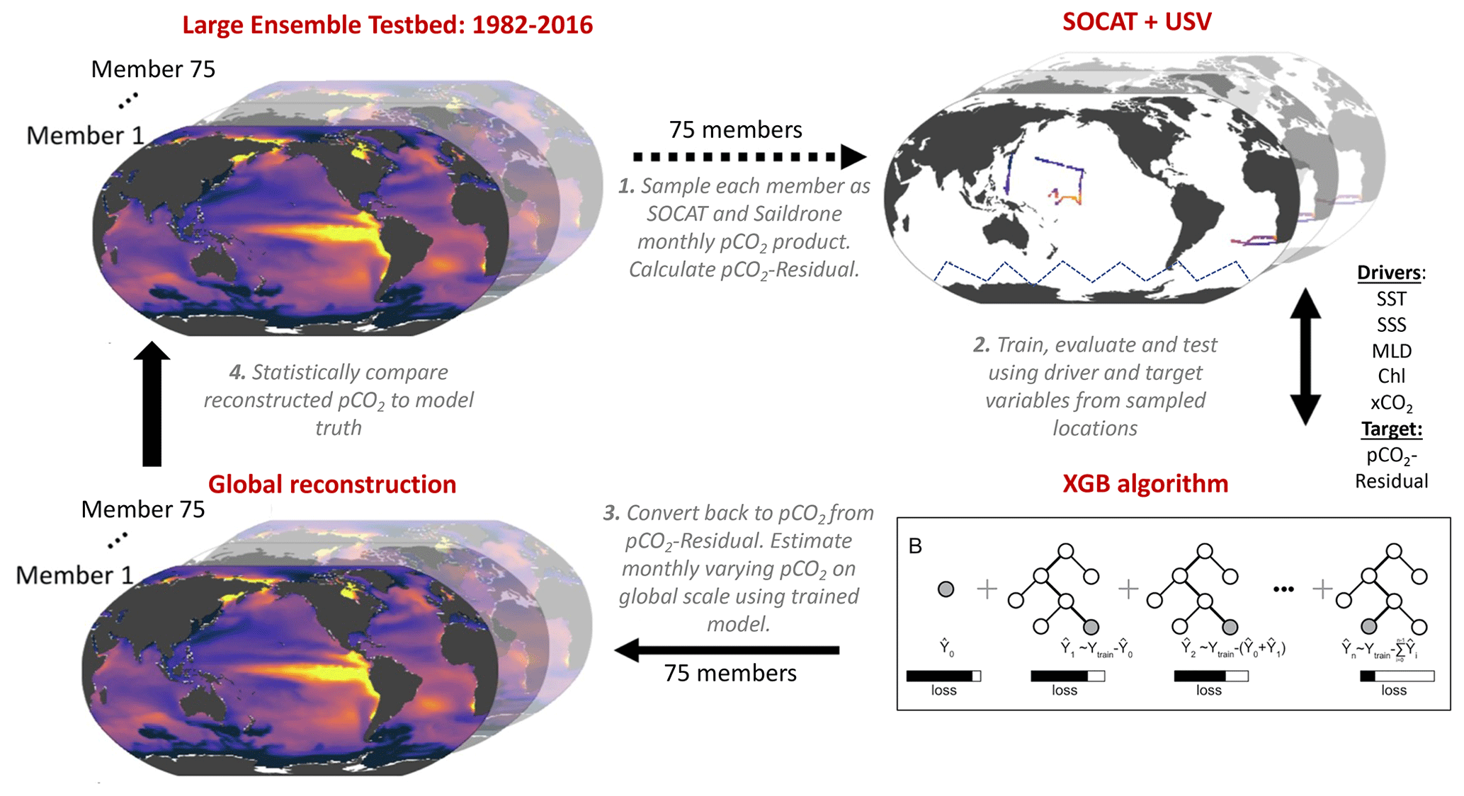
Figure 1 Schematic of the large ensemble test bed (LET; modified from Gloege et al., 2021). (1) Surface ocean pCO₂ from each of the 75 model members is sampled in space and time mimicking real-world SOCAT and Saildrone USV observations (see Fig. 2; Table 1; Sect. 2.4). Prior to algorithm processing, pCO₂-Residual is calculated (Sect. 2.2). (2) The pCO₂-Residual (target variable) and co-located driver variables (i.e., SST, SSS, MLD, Chl and xCO₂) sampled from the test bed are processed by the XGBoost (XGB) algorithm (Sect. 2.2). (3) Based on the full coverage of driver variables, pCO₂-Residual is reconstructed globally. This process is repeated 75 times, individually for every single test bed model member. The temperature component (pCO₂-T) is then added back to the pCO₂-Residual for each value. (4) The globally reconstructed pCO₂ is evaluated against the model truth at all 1°×1° grid cells. SST: sea surface temperature. SSS: sea surface salinity. MLD: mixed layer depth. Chl: chlorophyll. xCO₂: atmospheric concentration of CO₂.

2.2 The pCO₂-Residual approach

We used the pCO₂-Residual approach following Bennington et al. (2022a), which removes the well-studied direct effect of temperature on pCO₂ from the LET model output before algorithm processing. Temperature has both direct and indirect effects on surface ocean pCO₂. The direct effect of temperature, due to solubility and chemical equilibrium, is that an increase in temperature directly causes an increase in pCO₂ (Takahashi et al., 1993). Indirectly, temperature changes are associated with biological production and wintertime vertical mixing, and these processes tend to result in opposing pCO₂ changes. To build reconstruction algorithms through the data-driven training that occurs in ML, the statistics in all other algorithms developed to date must identify a function that disentangles these competing effects of SST on pCO₂. Here, the algorithm is assisted by removing this known temperature effect, and it must therefore only learn the pCO₂ impacts from biogeochemical drivers. The pCO₂-Residual method leads to physically understandable connections between the input data and the output (Bennington et al., 2022a), which mitigates to some degree “black box” concerns typically associated with ML algorithms (Toms et al., 2020). Bennington et al. (2022a) demonstrate higher skill for reconstructions using pCO₂-Residual as the target variable as opposed to pCO₂ (Fig. S1 in Bennington et al., 2022a), indicating that the removal of the temperature-driven component enhances the performance of the method. Further, the pCO₂-Residual method has been shown to perform slightly better against independent observations than other common mapping methods (Bennington et al., 2022a). A brief description is provided here, but for further details, see Bennington et al. (2022a).

The temperature-driven component of pCO₂ (pCO₂-T) is calculated using the following equation:

$$p{\mathrm{CO}}_{\mathrm{2}}\text{-}T=p{\mathrm{CO}}_{\mathrm{2}}^{\mathrm{mean}}\times \exp [\mathrm{0.0423}\times (\mathrm{SST}-{\mathrm{SST}}^{\mathrm{mean}}\left)\right],$$

where pCO${}_{\mathrm{2}}^{\mathrm{mean}}$ and SST^mean are the long-term means of surface ocean pCO₂ and temperature, respectively, using all 1°×1° grid cells from the test bed. Alternative sources of mean pCO₂ were assessed by Bennington et al. (2022a), but they found no significant impact on the test statistics or reconstructed pCO₂. Once pCO₂-T is determined, pCO₂-Residual is calculated as the difference between pCO₂ and the calculated pCO₂-T:

$$p{\mathrm{CO}}_{\mathrm{2}}\text{-Residual}=p{\mathrm{CO}}_{\mathrm{2}}-p{\mathrm{CO}}_{\mathrm{2}}\text{-}T.$$

Prior to algorithm processing, pCO₂-Residual values >250 and $<-\mathrm{250}$ µatm from the test bed were filtered out, targeting values that are not representative of the real ocean. The majority of the pCO₂-Residual values that were filtered out correspond to high pCO₂ values above the maximum value in SOCAT (816 µatm; Stamell et al., 2020). The excluded data points (less than 0.2 % per member) mostly occurred in the output from the CanESM2 model and were restricted geographically, predominantly along the western coastline of South America.

The eXtreme Gradient Boosting method (XGB; Chen and Guestrin, 2016) is used to develop an algorithm that allows driver variables (i.e., SST, SSS, Chl a, MLD and xCO₂) to predict the pCO₂-Residual (Fig. 1; Step 2). The pCO₂-Residual and associated feature variables are split into validation, training and testing sets. The test and validation sets each account for 20 % of the data, leaving 60 % for training. The validation set is used to optimize the algorithm hyperparameters, which define the architecture of decision trees used in the model. The training set is used to build the decision trees in XGB, while the test set is used to evaluate the performance of the final algorithm. The XGB algorithm for this study used 4000 decision trees with a maximum depth of six levels, and this was fixed for all experiments (see Sect. S1 in the Supplement). For the final reconstruction of surface ocean pCO₂ across all space and time points, the previously calculated pCO₂-T values are added back to the reconstructed pCO₂-Residual (Fig. 1; Step 3).

The full XGB process, including (1) training, evaluating and testing and (2) reconstructing globally at a monthly resolution, was repeated individually for each LET member. This process therefore provided a total of 75 unique reconstruction vs. model truth pairs, which can be statistically compared (Fig. 1; Step 4).

2.3 Statistical analysis in the test bed

The statistical comparisons between the test set and the reconstructions are equivalent to what would be derived using real-world data (“seen” values). Here, we calculate error statistics based on the full reconstruction (pCO₂ from all 1°×1° grid cells of the test bed, except for those masked or filtered out). In the full reconstruction, ∼99 % of the data do not correspond to SOCAT or Saildrone USV observations used to train the algorithm (Fig. S1 in the Supplement). Training data would ideally be removed before performance evaluation, but since the training data represent only ∼1 %, the impact of not removing them is negligible (Fig. S2). A suite of statistical metrics can be used to compare the reconstruction to the model truth in order to assess how well the algorithm can extrapolate from sparse data to full-field coverage (Fig. 1; Step 4). In this study, we focus on the bias and root-mean-squared error (RMSE). Bias is calculated as mean prediction minus mean observation (i.e., pCO₂ predicted by XGB subtracted by the pCO₂ model truth) and is a measure of over- or underestimation in the reconstructions. RMSE measures the magnitude of the predicted error and is calculated as the square root of the mean of the squared errors. We focus our discussion on the mean across 75 members of the test bed for bias and the RMSE. The spread across test bed ensemble members is non-negligible and will be the focus of future work; here, we present the test bed spread primarily in the Supplement.

2.4 Overview of sampling patterns and model runs

First, we sampled target and driver variables from the LET based on sampling distributions equivalent to that of the SOCAT database (“SOCAT baseline”). Then, we combined the SOCAT baseline with test bed output representing additional Saildrone USV coverage in the Southern Ocean. The additional Southern Ocean coverage was based on (1) the Sutton et al. (2021) sampling campaign from 2019 (“one-latitude” track) and (2) realistic potential future meridional USV observations (“zigzag” track) (see Sect. 2.4.2; Fig. 2). We performed a total of 10 experimental runs (Table 1). These represent different sampling approaches, including (1) repeating USV sampling over a period of 5 or 10 years, (2) varying the number of USVs and thus the total number of monthly 1°×1° observations, and (3) restricting all observations to Southern Hemisphere winter months. By comparing the different runs, we can assess whether or not certain targeted sampling strategies in the Southern Ocean can improve surface ocean pCO₂ ML reconstructions. As discussed above, the LET runs until 2016 only (Gloege et al., 2021). Saildrone USV observations were therefore sampled from the test bed starting in year 2006 or 2007 (for the 10-year sampling) or 2012 (for the 5-year sampling) and lasting until 2016, i.e., the final year of the test bed.

2.4.1 One-latitude runs

Out of the 10 experimental runs, 6 include the one-latitude track (Table 1). The 2019 Saildrone USV journey (Sutton et al., 2021) covered an 8-month period, from January to August. Since the USV was recovered in early August, it did not cover the entire Southern Hemisphere winter (Fig. S3). We repeated this one-latitude 8-month sampling pattern for 5 years (5Y_J-A; 2075 observations) and 10 years (10Y_J-A; 4150 observations). To evaluate year-round (YR) coverage, the 8-month sampling period (January–August) was shifted by 1 month each year for 10 years (10Y_YR; 4150 observations). To evaluate the impact of increased sampling, the 2019 Saildrone USV track was repeated 12 times with incremental offsets of 1° from the original track, covering an additional 6° north and south (Fig. S4). This “high-sampling” run (x13_10Y_J-A; 44 250 observations) represents a total of 13 USVs. We also performed an additional 13 USV runs but including observations from Southern Hemisphere winter (W) months only (x13_10Y_W; 25 395 observations). Finally, considering the cost of deploying 13 USVs, a downscaled multiple-USV winter-only run was tested, including five USVs sampling over a period of 5 years (x5_5Y_W; 5022 observations). This run covers an additional 2° north and south from the original USV track.

2.4.2 Zigzag runs

Of the 10 experimental runs, 4 represent realistic potential meridional sampling in the Southern Ocean (zigzag tracks; Table 1), as suggested by Djeutchouang et al. (2022). Saildrone USVs can operate at a speed capable of covering the spatial extent of meridional gradients in the Southern Ocean (Djeutchouang et al., 2022). However, Saildrone USVs are solar-powered, and thus, their range is restricted by the availability of solar radiation. To account for this and maintain a realistic sampling scenario, sampling occurs only to a maximum latitude of 55° S in these experiments. This alternative sampling pattern represents USVs sailing west to east in a north–south zigzag pattern covering 40 and 55° S for every 30° of longitude (Fig. 2). We created two scenarios. For the first scenario, every 30° of longitude from 40 and 55° S is visited every 3 months within a single year, as suggested by Lenton et al. (2006). Assuming an average Saildrone USV speed, this scenario represents four platforms equally spaced around the Southern Ocean. This sampling pattern was repeated for 10 years, with year-round coverage (Zx4_10Y_YR; 7600 observations), and for Southern Hemisphere winter months only (Zx4_10Y_W; 2500 observations). The second scenario represents a high-sampling strategy, where every 30° of longitude from 40 and 55° S is visited approximately monthly. This can be achieved by deploying 10 platforms equally spaced around the Southern Ocean, running at an average Saildrone USV speed. This sampling pattern is repeated for 5 years, sampling year-round (Z_x10_5Y_YR; 11 400 observations) and during Southern Hemisphere winter months only (Z_x10_5Y_W; 3800 observations).

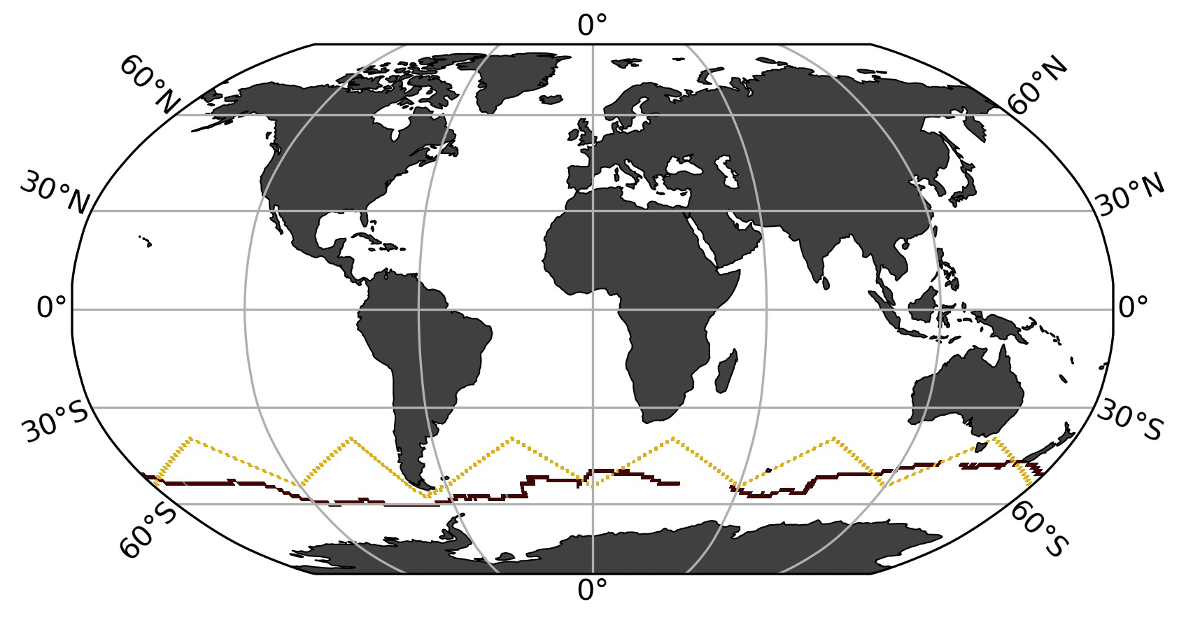
Figure 2 Saildrone uncrewed surface vehicle (USV) tracks representing the first circumnavigation around Antarctica from 2019 in maroon (one-latitude track; Sutton et al., 2021) and an alternative virtual route with meridional coverage (zigzag track).

Table 1 Overview of the different sampling experiments tested in this study, mean bias and RMSE (in µatm) for various time periods, and latitude bands for all runs. Bold values represent the best score for each category. One-lat: one-latitude track, which incorporates the Saildrone USV route from Sutton et al. (2021). Zigzag: potential meridional sampling. Additional observations: number of 1°×1° monthly Saildrone USV observations in addition to SOCAT. J–A: January–August. YR: year-round. W: Southern Hemisphere winter. ×4, ×5, ×10 and $\times \mathrm{13}=$ 4, 5, 10 and 13 USVs. SO winter: Southern Ocean winter months, i.e., June, July and August, and also including September. not applicable – n/a.

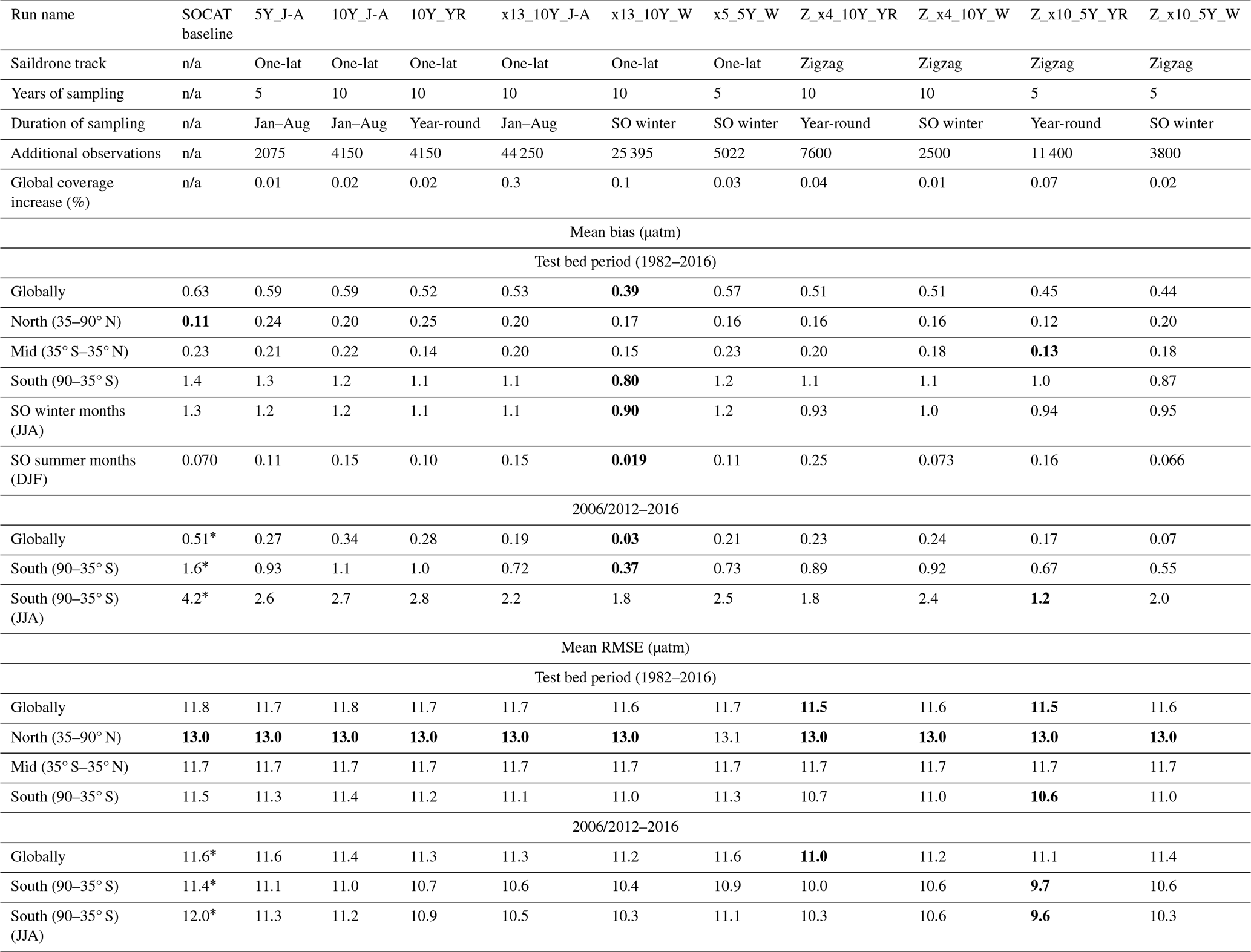
^* Average value of the mean for 2006–2016 and 2012–2016. The global coverage increase was calculated based on the total number of available 1982–2016 monthly 1°×1° observations from SOCAT (262 204 observations) and the large ensemble test bed (17 290 470 observations).

2.5 Air–sea CO₂ flux

To assess the global ocean carbon sink associated with our pCO₂ reconstructions, air–sea CO₂ exchange was calculated for 1985 onward. Here, we computed air–sea CO₂ fluxes using the bulk formulation with the Python package SeaFlux 1.3.1 (https://github.com/lukegre/SeaFlux, last access: August 2023; Gregor and Fay, 2021; Fay et al., 2021). We calculated global and Southern Ocean flux in the same manner for (1) the test bed model truth, (2) the SOCAT baseline and (3) the 10 experimental USV runs.

The net sea–air CO₂ flux was estimated using

$$\mathrm{flux}=k_w\cdot \mathrm{sol}\cdot (p{\mathrm{CO}}_{\mathrm{2}}^{\mathrm{ocn}}-p{\mathrm{CO}}_{\mathrm{2}}^{\mathrm{atm}})\cdot (\mathrm{1}-\mathrm{ice}),$$

where k_w is the gas transfer velocity; sol is the solubility of CO₂ in seawater (in units of mol m⁻³ µatm⁻¹); pCO${}_{\mathrm{2}}^{\mathrm{ocn}}$ is the partial pressure of surface ocean carbon (in µatm), either from the model truth or from the reconstructions; and pCO${}_{\mathrm{2}}^{\mathrm{atm}}$ (in µatm) is the partial pressure of atmospheric CO₂ in the marine boundary layer. For GFDL, we used the direct model output of pCO${}_{\mathrm{2}}^{\mathrm{atm}}$, while for CESM and CanESM2, pCO${}_{\mathrm{2}}^{\mathrm{atm}}$ was calculated individually as the product of surface xCO₂ and sea level pressure (the contribution of water vapor pressure was corrected for in CESM). Finally, to account for the seasonal ice cover in high latitudes, the fluxes were weighted by 1 minus the ice fraction (ice), i.e., the open-ocean fraction.

Winds have the largest impact on flux calculations (Fay et al., 2021), and temporally high-resolution output is not available for the LET. Monthly output is available, but this is not sufficient for the flux calculation due to the square dependency of wind speed (Wanninkhof, 2014). Given the necessity to use observed winds, for consistency, we use observations for all necessary variables for the flux calculation. Inputs to the calculation include EN.4.2.2 salinity (Good et al., 2013), SST and ice fraction from NOAA Optimum Interpolation Sea Surface Temperature V2 (OI SST v2) (Reynolds et al., 2002), and surface winds and associated wind scaling factor from the European Centre for Medium-Range Weather Forecasts (ECMWF ERA5) sea level pressure (Hersbach et al., 2020). Results presented show the global and Southern Ocean (<35° S) fluxes in units of Pg C yr⁻¹.

Note that reconstructions of pCO₂ for the SOCAT baseline and the experimental USV runs are limited in their spatial extent to the open ocean (see Sect. 2.1; excluding coastal areas, the Arctic Ocean and marginal seas). The same mask was thus also applied when calculating the flux of the model truth, prior to comparison with the reconstructions.

3 Results

3.1 Performance metrics for the SOCAT baseline reconstruction

The mean bias for the entire test bed period (i.e., 1982–2016) is 0.63 µatm globally (Fig. 3a) and 1.4 µatm for the Southern Ocean (<35° S; Table 1). Bias is much closer to 0 for the mid-latitudes (between 35° S and 35° N; 0.23 µatm) and northern latitudes (>35° N; 0.11 µatm) (Fig. 3a). There is a significant difference in bias in the case of Southern Hemisphere winter months (June, July, August) versus summer months (December, January, February), with a global mean bias (for 1982–2016) of 1.3 µatm compared to 0.07 µatm, respectively (Table 1), due to the sparseness of SOCAT observations from the Southern Hemisphere during the harsh winter season (Fig. S5a). The mean RMSE for the entire test bed period (i.e., 1982–2016) is 11.8 µatm globally (Fig. 3b) and 11.5 µatm for the Southern Ocean (Table 1). RMSE is highest in the eastern tropical and southeastern Pacific Ocean and in the Southern Ocean, where the algorithm generally overestimates pCO₂ (i.e., positive bias; Fig. 3a), with some exceptions in the Atlantic section. This is consistent with the areas significantly undersampled by SOCAT (Fig. S5b). Except in these areas, RMSE and bias are generally low (close to 0) in the open ocean but show higher values along coastlines (Fig. 3b). The predicted pCO₂ is thus more accurate in areas similar to and surrounding the SOCAT observations (i.e., monthly 1°×1° grid cells equivalent to SOCAT coverage but sampled from the LET). Figure 3 shows mean bias and RMSE for the full reconstruction (see Sect. 2.3), but note that there is a statistically significant difference between the training and testing set errors (Fig. S6). This indicates potential overfitting in our ML model (i.e., higher errors for the “unseen” reconstruction) and that further tuning of the hyperparameters could increase generalization skill (see Sect. S1).

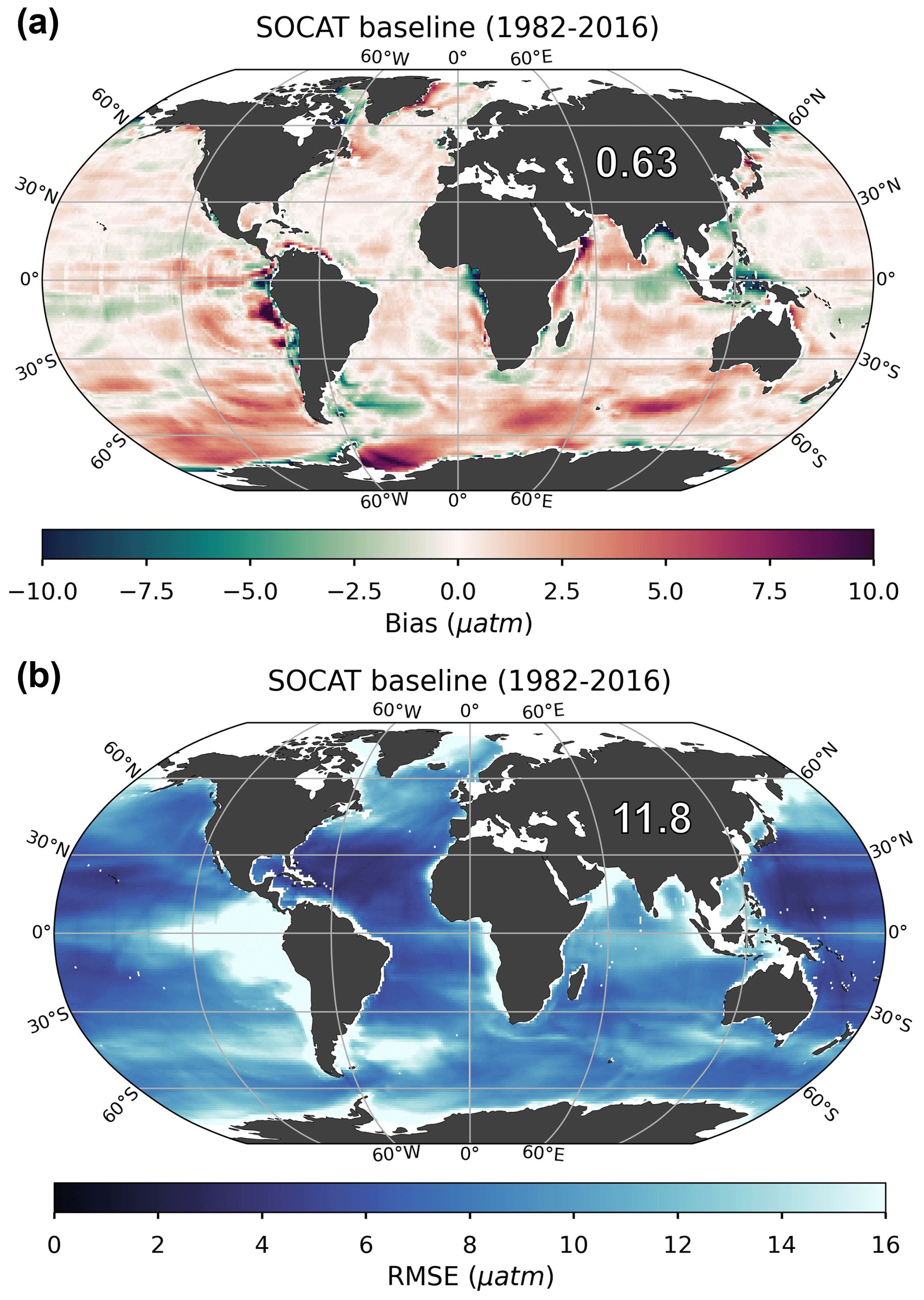
Figure 3 Bias (a) and root-mean-squared error (RMSE) (b) for the SOCAT baseline (i.e., no USV) over the period of 1982 through 2016. The global mean bias and RMSE are 0.63 and 11.8 µatm, respectively. Note that only the open ocean was considered in the reconstruction, so several areas were masked out prior to algorithm processing, such as the Arctic Ocean, coastal areas and marginal seas (no data; white areas in figures).

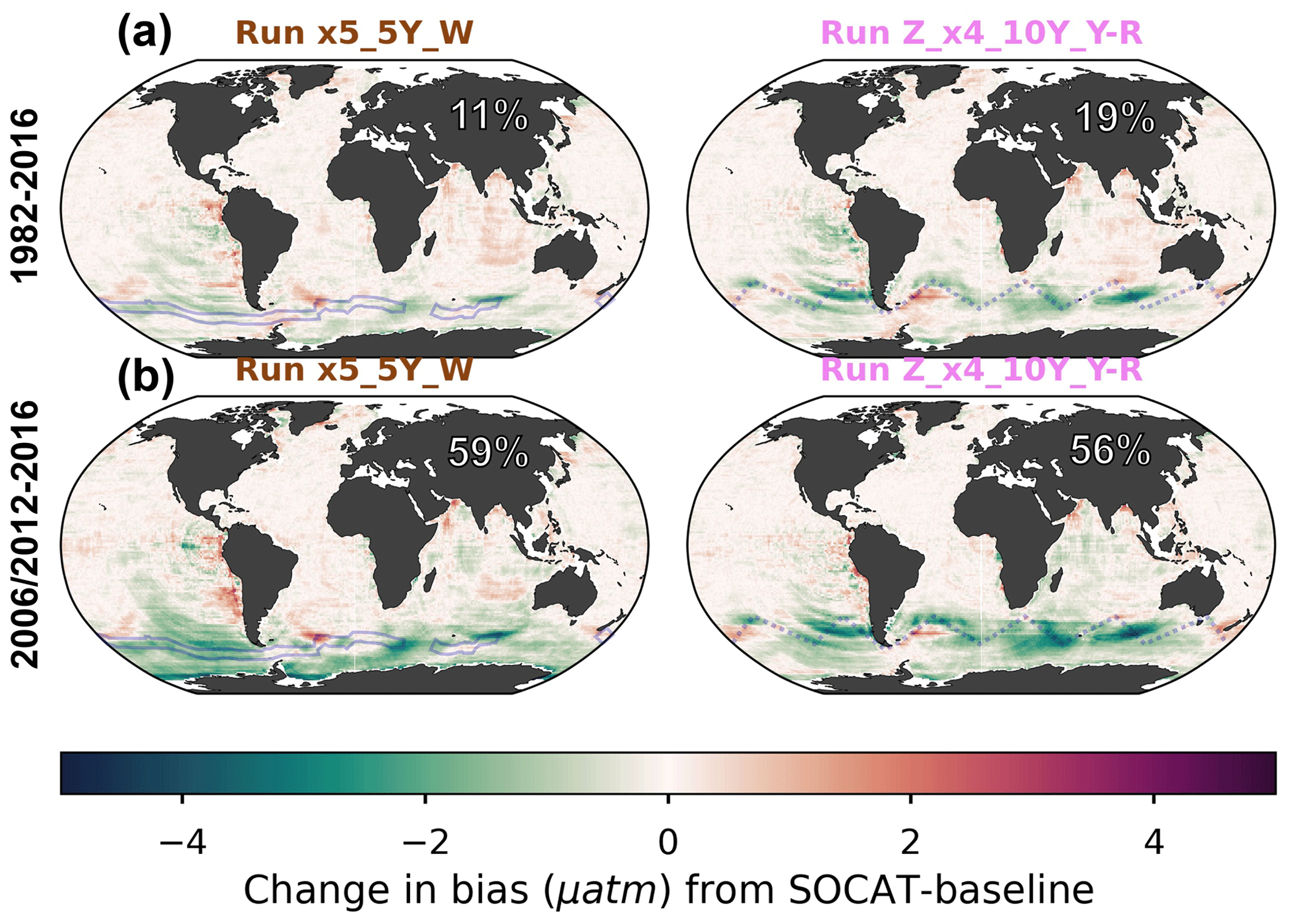
Figure 4 Change in bias when comparing runs x5_5Y_W and Z_x4_10Y_YR to the SOCAT baseline reconstruction averaged over the duration of the test bed period (a; 1982–2016) and the period of USV additions (b; 2006–2012 or 2012–2016). The percent global improvement in absolute bias is shown in each panel. The USV Saildrone tracks are shown in blue.

3.2 Reconstruction improvements with Saildrone USV additions

Our presentation of global maps is limited to runs x5_5Y_W (5022 monthly 1°×1° observations) and Z_x4_10Y_YR (7600 monthly 1°×1° observations). These runs were selected as they represent observational schemes that are realistic in the near-term future considering logistics and cost level, both non-meridional and meridional sampling, and different approaches to observing duration and seasonal coverage. For the remaining runs, equivalent maps can be found in the Supplement.

3.2.1 Bias

All Saildrone USV runs show a reduction in bias compared to the global mean 1982–2016 SOCAT baseline (Figs. 4a, S7). The improvement in bias is mainly due to lower reconstructed pCO₂ values at southern latitudes, where the SOCAT baseline reconstruction generally overestimates pCO₂ (Fig. 3a). The global mean bias for zigzag run Z_x4_10Y_YR is 0.51 µatm, a higher improvement (19 %) over the SOCAT baseline compared to the one-latitude run x5_5Y_W (11 % mean improvement; mean bias =0.57 µatm) (Fig. 4a; Table 1). Generally, the zigzag runs show higher improvements from the SOCAT baseline (19 %–31 % improvement; resulting mean bias of 0.44–0.51 µatm) compared to the one-latitude runs (7 %–19 % improvement; resulting mean bias of 0.52–0.59 µatm) (Fig. S7; Table 1). However, the one-latitude run x13_10Y_W that samples Southern Hemisphere winter months only stands out with the lowest global mean (1982–2016) bias of 0.39 µatm, representing a 39 % mean improvement from the SOCAT baseline (Table 1; Fig. S7). This run, however, has 3 and 5 times more observations (25 395) than Z_x4_10Y_YR and x5_5Y_W, respectively.

Compared to the entire test bed period, even larger improvements in global mean bias are shown for the period of Saildrone USV additions (2006–2016 and 2012–2016; Figs. 4a vs. 4b, S7 vs. S8). Compared to the SOCAT baseline, run x13_10Y_W results in a mean bias improvement of 95 %, while the remaining one-latitude runs and the zigzag runs show mean improvements up to 63 % and 86 %, respectively (Fig. S8). The spread in mean bias (2006/2012–2016) across the 75 test bed members for each experiment is shown in Fig. S9.

Perhaps surprisingly, there is not a strong connection between the global or Southern Ocean mean bias and the number of added USV observations (Fig. 5). The one-latitude high-sampling run x13_10Y_J-A (44 250 observations) shows similar mean bias or is outperformed by all zigzag runs and the one-latitude runs that restrict sampling to Southern Hemisphere winter months (i.e., x5_5Y_W and x13_10Y_W).

Considering the change in bias from year to year, the SOCAT baseline shows positive bias at all latitudes in the beginning of the test bed period, before improvement occurs around 1990 (Fig. 6a). This is consistent with increasing SOCAT sampling with time for the period considered here (i.e., up to 2016; Fig. S5c). As SOCAT observations are biased towards the Northern Hemisphere (Fig. S5a, b), bias in the Southern Ocean (<35° S) increases significantly starting in the 2000s and remains high until the end of the test bed period (Fig. 6a). By adding USV sampling, bias in the Southern Ocean improves over the SOCAT baseline around year 2000 (Figs. 6b–d; S10), up to 6–12 years before to the introduction of additional samples in either 2006 or 2012. This improvement is shown for the majority of the 75 ensemble members (Fig. S11). Run Z_x10_ 5Y_W, which has the lowest mean bias out of the zigzag runs (Fig. 5), shows improvement even further back in time, until the beginning of the test bed period (Fig. S10). While the annual mean bias of the zigzag runs varies rather consistently, there is a larger spread across the one-latitude runs (Fig. 6d).

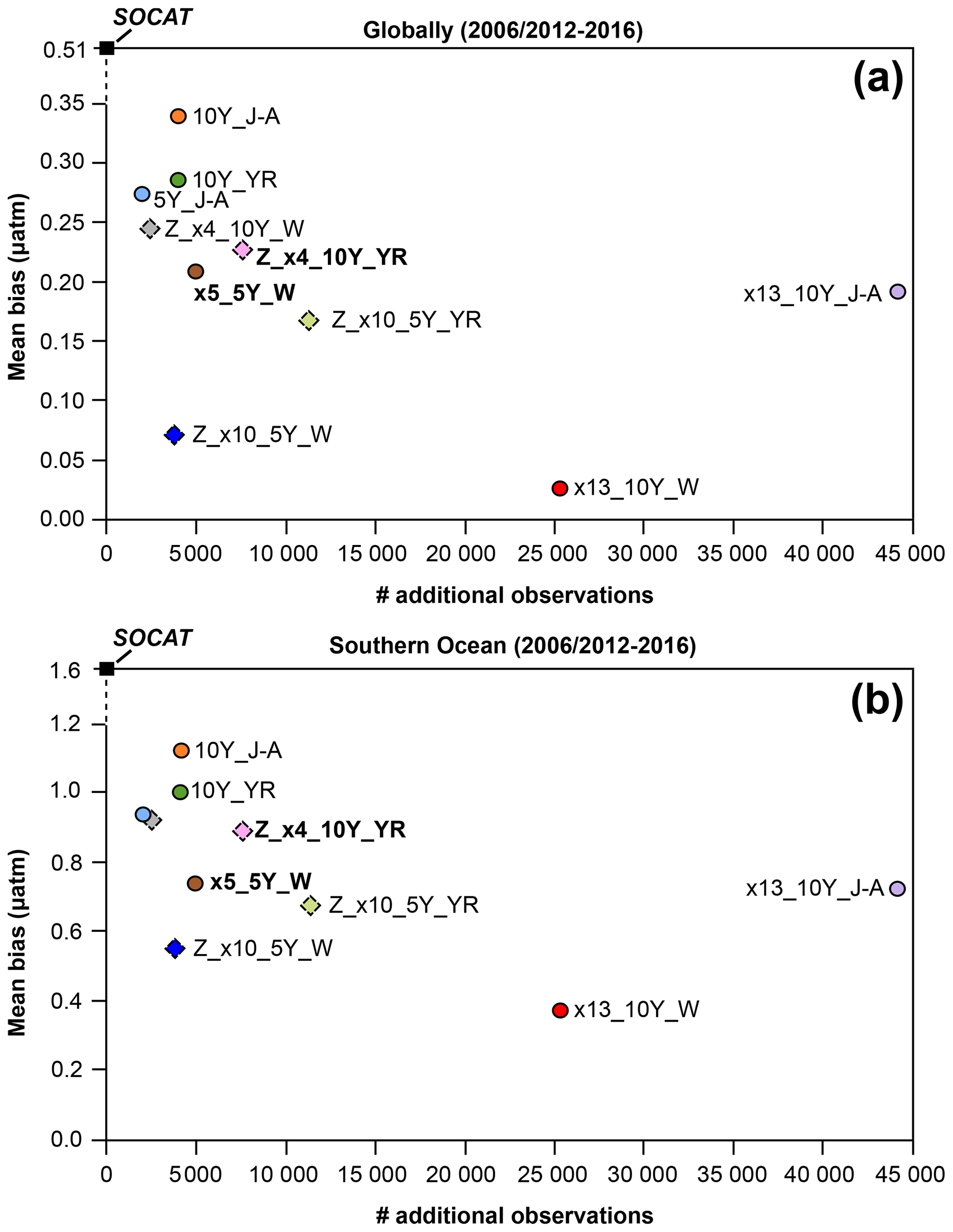
Figure 5 Mean bias globally (a) and for the Southern Ocean (b) for the duration of Saildrone USV sampling (2006–2016 or 2012–2016) for all runs presented in Table 1. Circles represent runs using the one-latitude track, while diamonds represent zigzag runs. Runs highlighted in bold correspond to the two selected runs mapped in Figs. 4, 6, 7 and 9. Global (0.51 µatm) and Southern Ocean (1.6 µatm) bias values shown for the SOCAT baseline (black squares) represent a mean of values for 2006–2016 (global mean of 0.52 µatm; Southern Ocean mean of 1.63 µatm) and 2012–2016 (global mean of 0.51 µatm; Southern Ocean mean of 1.56 µatm). The number of monthly 1°×1° USV observations in addition to SOCAT is denoted by # additional observations. Box plots illustrating the spread across the 75 ensemble members are shown in Fig. S9.

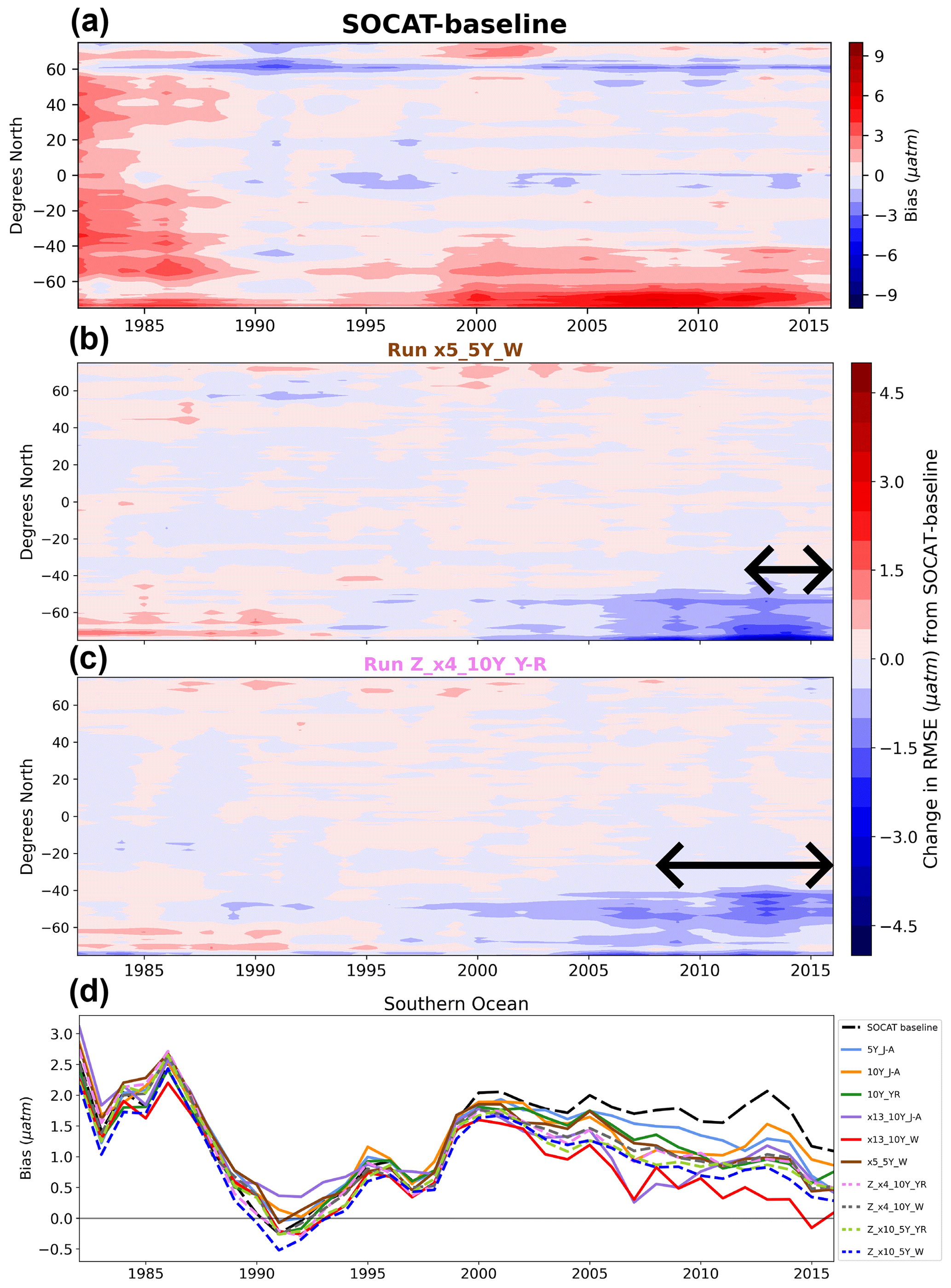
Figure 6 Zonal mean and annual mean Hovmöller of bias for the SOCAT baseline (a). Change in bias for runs x5_5Y_W (b) and Z_x4_10Y_YR (c) compared to the SOCAT baseline shown in panel (a). Improvement in bias in the Southern Ocean expands back in time well beyond the duration of USV additions for both runs (shown by arrows in each panel). Annual mean bias for the Southern Ocean (>35° S) for all runs (d).

3.2.2 Root-mean-squared error (RMSE)

Similar to bias, improvements in RMSE are most significant during the period of USV additions and within the Southern Ocean (Fig. 7a vs. 7b). For the duration of USV additions, the one-latitude runs show improvements in global mean RMSEs of 0.5 %–3 % (0.1 %–1 % for 1982–2016), while the zigzag runs show higher improvements between 2 %–5 % (1 %–3 % for 1982–2016) (Figs. 7, S12, S13). Mean RMSE is further reduced in the Southern Ocean by up to 16 % and during Southern Hemisphere winter months (JJA) by up to 21 % (run Z_x10_5Y_YR; mean RMSE of 9.6 µatm; Table 1). There is minimal change in RMSE (or bias) during Southern Hemisphere summer months (DJF; Fig. S14). The two zigzag runs sampling year-round (Z_x4_10Y_YR and Z_ x10_5Y_YR) have the lowest RMSE values both globally and in the Southern Ocean (Fig. 8). The spread across the 75 test bed members for each experiment is shown in Fig. S15.

The zigzag runs, as well as the high-sampling one-latitude runs (i.e., x13_10Y_J-A and x13_10Y_W), show improvements compared to the SOCAT baseline from the initiation of sampling (Figs. 9, S16, S17). The year-round zigzag runs, however, show improvement in the Southern Ocean from the beginning of the test bed period (Figs. 9c, d, S16). RMSE improvements back in time are greater for all runs in the Southern Hemisphere winter months (Fig. S18).

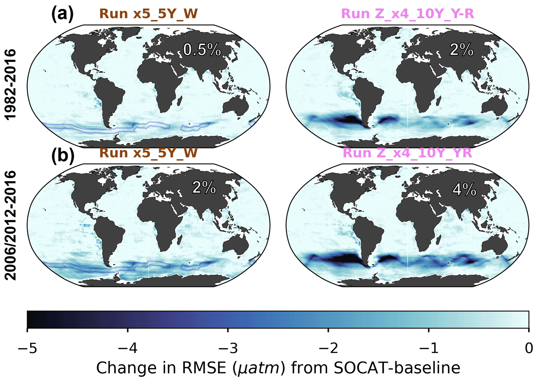
Figure 7 Change in RMSE when comparing runs x5_5Y_W and Z_x4_10Y_YR to the SOCAT baseline averaged over the duration of the test bed period (a; 1982–2016) and the period of Saildrone USV additions (b; 2006–2012 or 2012–2016). The percent global improvement is shown in each panel.

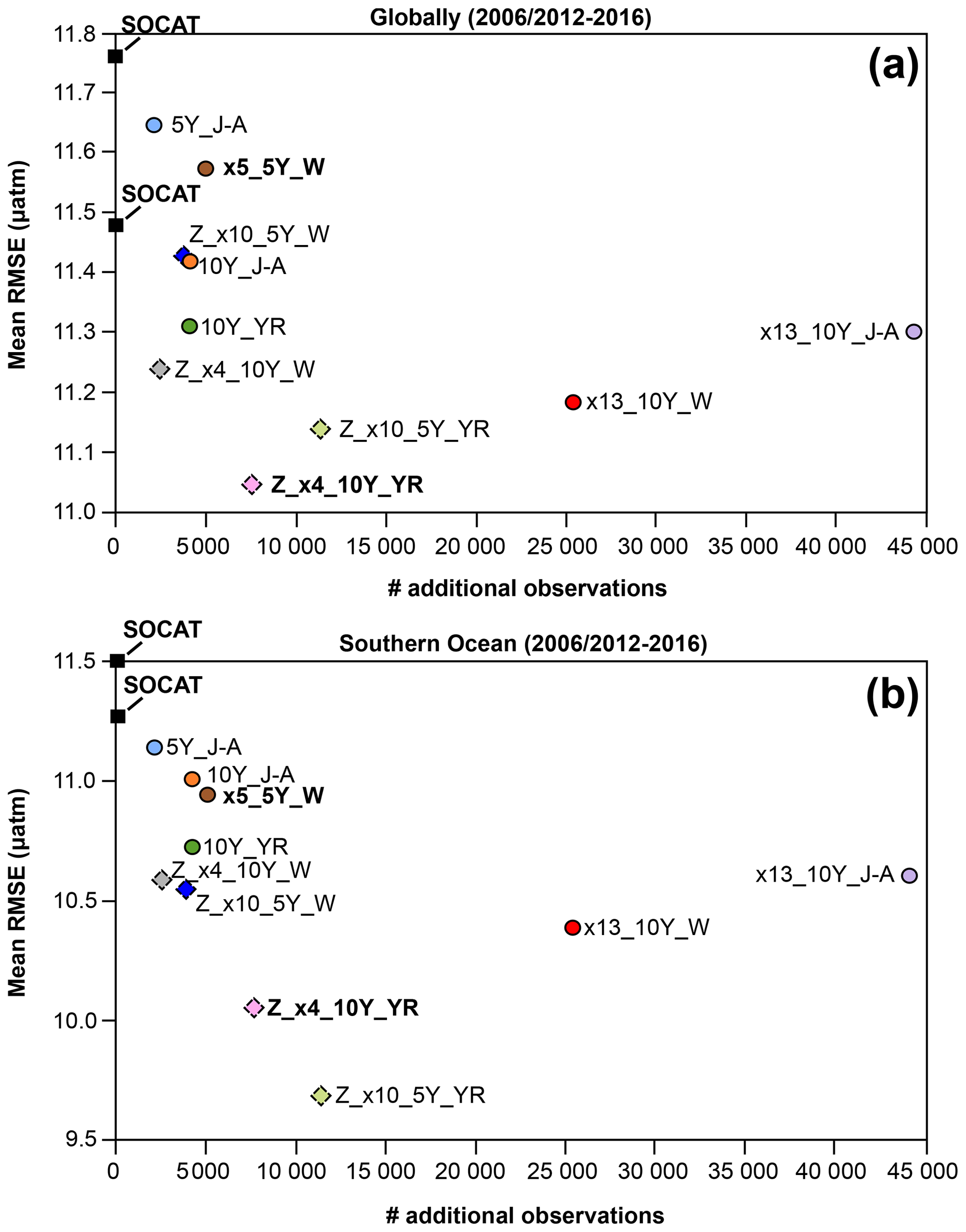
Figure 8 Mean RMSE globally (a) and for the Southern Ocean (<35° S; b) for the duration of Saildrone USV sampling (2006–2016 or 2012–2016) for all runs presented in Table 1. Circles represent runs using the one-latitude track, while diamonds represent zigzag runs. Runs highlighted in bold correspond to the two selected runs mapped in Figs. 4, 6, 7 and 9. RMSE values shown for the SOCAT baseline (black squares) represent a mean over 2006–2016 (global mean of 11.5 µatm; Southern Ocean mean of 11.3 µatm) and 2012–2016 (global mean of 11.8 µatm; Southern Ocean mean of 11.5 µatm). The number of monthly 1°×1° USV observations in addition to SOCAT is denoted by # additional observations. Box plots illustrating the spread across the 75 ensemble members are shown in Fig. S15.

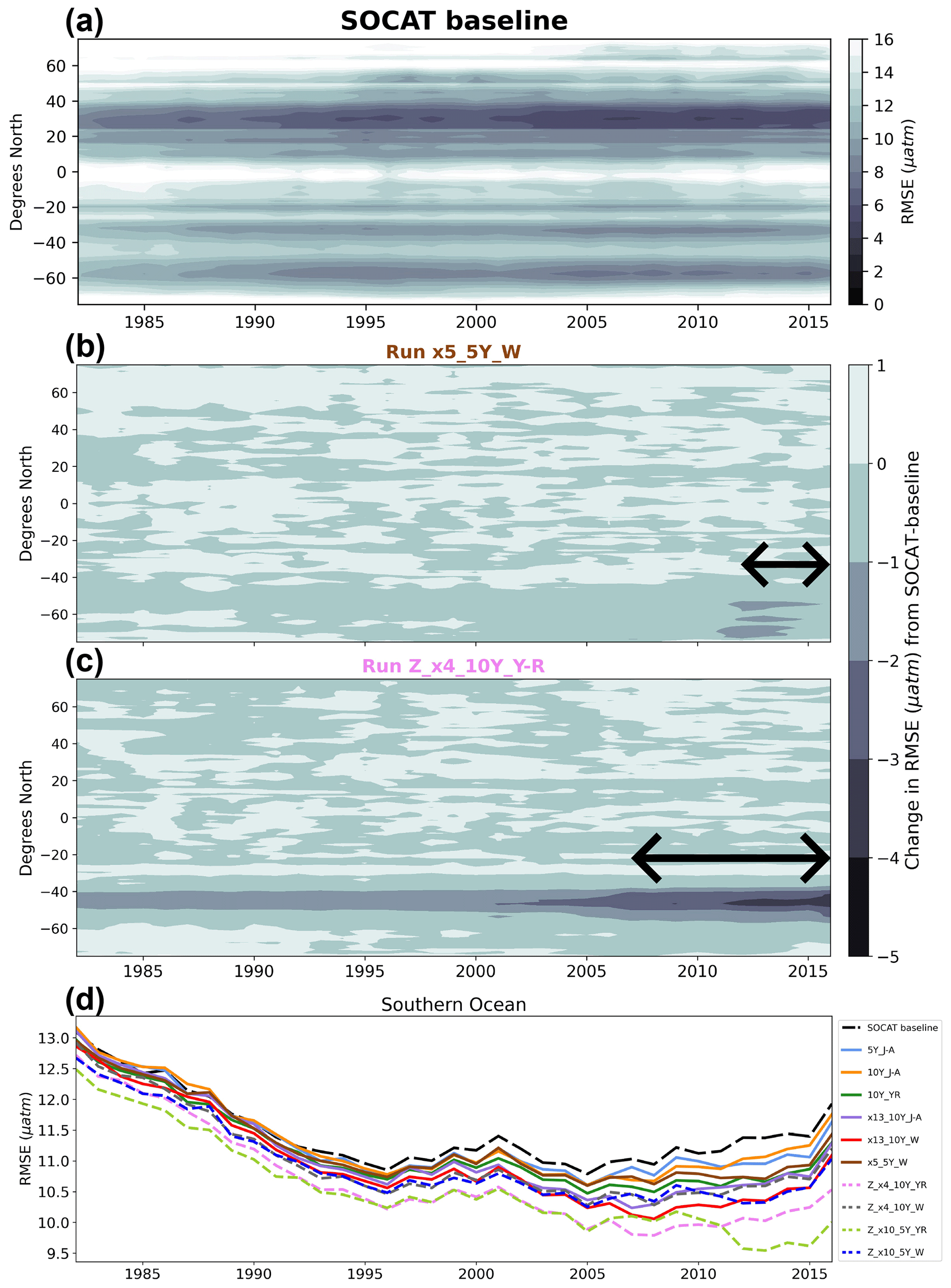
Figure 9 Zonal mean and annual mean Hovmöller of RMSE for the SOCAT baseline (a). Change in RMSE for run x5_5Y_W (b) and Z_x4_10Y_YR (c) compared to the SOCAT baseline. Run Z_x4_10Y_YR shows improvements in RMSE within the Southern Ocean, which expand well beyond the duration of Saildrone USV additions (shown by arrow in panel). Annual mean RMSE for the Southern Ocean (>35° S) for all runs (d).

3.3 Impact on the air–sea CO₂ flux with Saildrone USV additions

Air–sea flux was calculated in the same manner for both the ML reconstructions and the model truth, which allows for the isolation of the impact of different sampling strategies, as mediated by the pCO₂ reconstruction, on fluxes (see Sect. 2.5). These flux estimates are made to inform understanding of the errors that may exist in CO₂ flux estimates derived from pCO₂ reconstructions and how new sampling could address these errors. Flux estimates represent the average of the 75 members of the LET in each case and are not estimates of real-world fluxes.

Compared to the model truth, the SOCAT baseline reconstruction underestimates the global and Southern Ocean sink by 0.11–0.13 Pg C yr⁻¹ over 1982–2016 (Fig. 10; Table S1 in the Supplement). Regardless of the sampling pattern, adding Saildrone USV observations increases both the global and the Southern Ocean mean sink compared to the SOCAT baseline (Figs. 10, S19). The one-latitude runs show an increase of 0.01–0.03 Pg C yr⁻¹ (2 %–6 % strengthening) of the Southern Ocean sink (1982–2016), while the zigzag runs lead to an even stronger sink, increased by 0.04–0.06 Pg C yr⁻¹ (7 %–11 % strengthening) (Table S2). When averaging over the years of Saildrone USV sampling addition (i.e., 2006–2012 and 2012–2016), the Southern Ocean sink increases up to 0.09 Pg C yr⁻¹ (14 % strengthening) for the one-latitude runs and up to 0.1 Pg C yr⁻¹ (15 % strengthening) for the zigzag runs (Table S2). These same features are found for the global ocean (Fig. S19; Table S2).

All of the zigzag runs quite closely match both the global and the Southern Ocean model truth air–sea CO₂ flux for the duration of sample additions (Figs. 10, S19). Except for the first couple of years of sample addition for the high-sampling run x13_10Y_J-A, none of the one-latitude runs can match the model truth air–sea CO₂ flux; instead, they all underestimate the flux (Figs. 10, S19). The zigzag runs have impact on the air–sea flux from an earlier date, starting to pull the results away from the SOCAT baseline and toward the model truth already in the late 1990s, while the one-latitude runs do the same about a decade later (Figs. 10, S19).

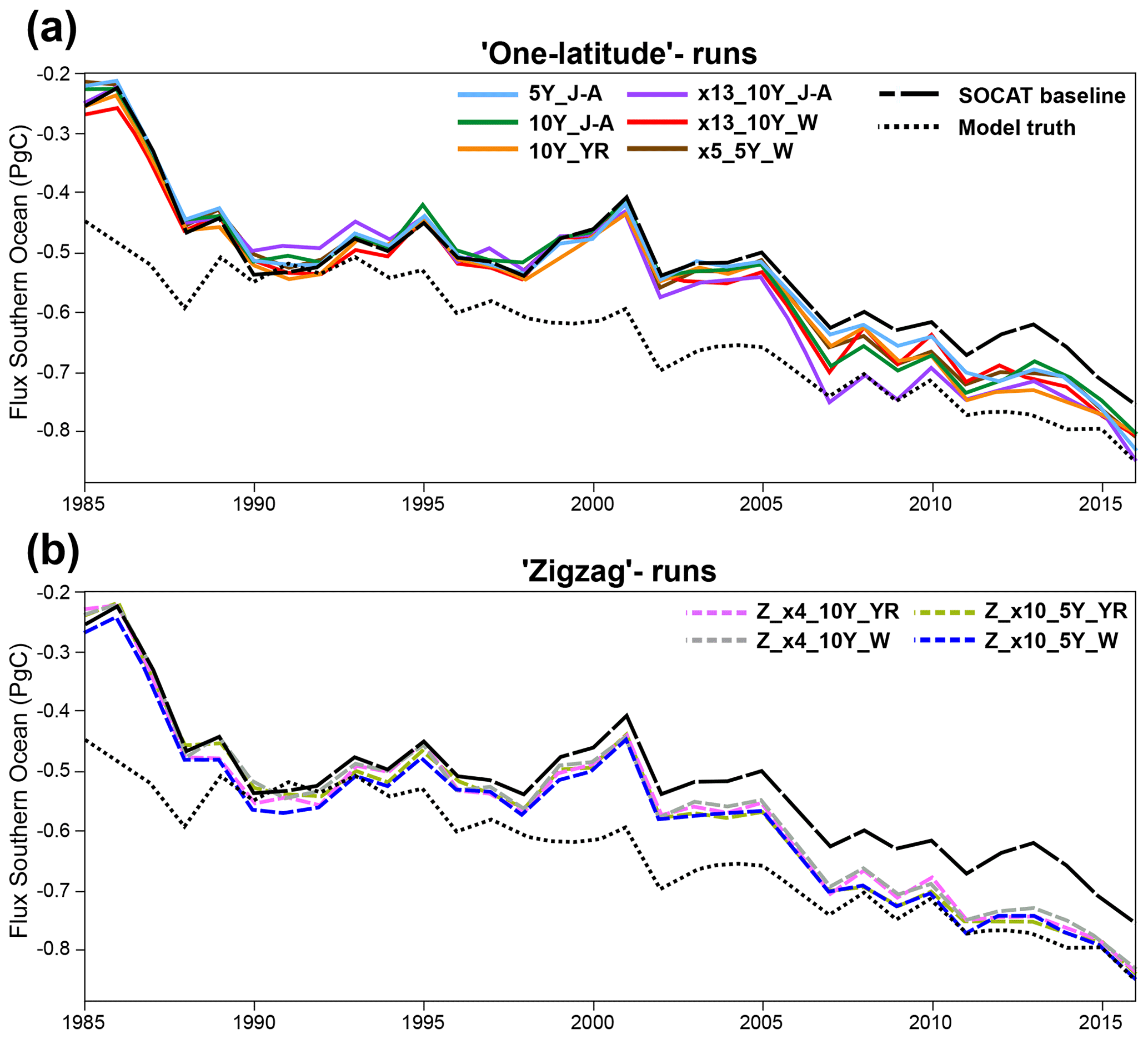
Figure 10 Southern Ocean (<35° S) annually averaged air–sea CO₂ flux for the SOCAT baseline (dashed black line) and model truth (dotted black line) for one-latitude runs (a; solid lines) and zigzag runs (b; dashed lines).

4 Discussion

We have tested the pCO₂-Residual reconstruction method with the large ensemble test bed (LET) to estimate its fidelity and understand how new samples could increase skill. We find that, regardless of the chosen Saildrone USV sampling pattern, the reduction in mean bias and mean RMSE compared to the SOCAT baseline is most prominent within the Southern Ocean, (<35° S) during the period of which Saildrone USV observations were added (Figs. 4, 6, 7, 9). However, it is important to mention that the additional Southern Ocean sampling also impacts (improves) the pCO₂ reconstructions globally (Figs. 5a, 8a). Based on our experiments, a combination of factors improves global and Southern Ocean pCO₂ reconstructions, including the type of sampling pattern and seasonality of sampling and, to some extent, the number of additional observations. Importantly, increasing the number of observations or duration of sampling (5 vs. 10 years) is not the sole determining factor for improving the reconstructions (Figs. 5, 8). This is best demonstrated by the high-sampling run x13_10Y_J-A (44 250 observations), which does not provide significantly better reconstructions or is even outperformed by runs with 2–18 times fewer observations. The runs that produce lower mean RMSE do include data throughout Southern Hemisphere winter (Fig. 8). Run x13_10Y_J-A does not include more than a few observations in the month of August, as it follows the temporal pattern of the real-world one-latitude Saildrone USV expedition (Figs. S3, S4; Sutton et al., 2021). The one-latitude runs 10Y_J-A and 10Y_YR are directly comparable in terms of sample duration, spatial extent and number of observations (Table 1), but the latter, which covers all months, always shows lower mean RMSE and bias (Figs. 5, 6d, 8, 9d). These examples attest to the importance of addressing the issue of significant undersampling in the Southern Ocean during the winter season (Fig. S5a).

Another important comparison is between the one-latitude run x5_5Y_ W (5022 observations) and zigzag run Z_x10_5Y_W (3800 observations) that both sample during Southern Hemisphere winter months over a 5-year period (Table 1), where the zigzag run consistently performs better even though it includes fewer observations (Figs. 5, 8). Most of the runs that perform similarly to, or outperform, the abovementioned high-sampling run x13_10Y_J-A (44 250 observations) sample in a zigzag pattern. Out of all 10 runs, the year-round zigzag runs (Z_x4_10Y_YR and Z_x10_5Y_YR) are most able to reduce the mean error, as shown by the lowest RMSE values (Figs. 8, 9d). A recent study performed similar sampling experiments, as shown here, by comparing sampling from different types of autonomous platforms to a SOCAT baseline (Djeutchouang et al., 2022). They emphasized the importance of capturing the significant differences in pCO₂ that exist across meridional gradients during summer and winter months (up to 15 µatm; Djeutchouang et al., 2022). The meridional coverage provided by the zigzag runs could explain why these runs generally outperform the one-latitude runs in our study and show significant reduction in both RMSE and bias even though the global pCO₂ data density is raised by as little as 0.01 %–0.07 %.

The greatest reduction in mean bias out of all runs is shown by run x13_10Y_W (Figs. 5, 6d), which represents one-latitude high-sampling (i.e., 25 395 observations) during Southern Hemisphere winter months only. This sampling strategy thus seems to have a higher ability to reduce the ML model's tendency to overestimate pCO₂ in the Southern Ocean compared to any of the meridional (zigzag) runs. However, it should be noted that run x13_10Y_W covers areas south of 55° S (Fig. S4), and its improvement in mean bias (and mean RMSE) is particularly prevalent at these high latitudes (e.g., Figs. S8, S10, S13, S16). Whether or not this run is, in fact, feasible with current or future technology is uncertain, as parts of the southernmost tracks potentially cover the Southern Ocean ice zone (Fig. S20), and solar radiation for solar-powered platforms and sensors becomes very limited during winter south of 55° S. Furthermore, this particular sampling strategy requires 13 USVs and so would be the most costly of the observing scenarios. Although run x13_10Y_W demonstrates the highest reduction in mean bias out of all runs, the zigzag runs still reduce absolute mean bias (for 2006/2012–2016) in the Southern Ocean by 44 %–65 % (vs. 77 % for run x13_10Y_W).

Overall, the zigzag runs include significantly fewer observations, require fewer USVs, collect samples over the same duration (or even half the time, as run x13_10Y_W), cover areas north of 55° S and within the ice-free zone, and show major improvement in the reconstruction of pCO₂ (attested to by reductions in both bias and RMSE). The zigzag runs also closely match both the global and the Southern Ocean model truth air–sea CO₂ flux for the duration of sample additions (Figs. 10, S19). It also appears that the zigzag runs generally have a greater impact on both the pCO₂ reconstruction and the air–sea flux further back in time and start to deviate from the SOCAT baseline earlier compared to the one-latitude runs (Figs. 6, 9, 10, S10, S16, S18, S19). Even the zigzag scenarios with the least number of USVs (e.g., Z_x4_10Y_YR) reduce Southern Ocean reconstruction absolute mean (2006–2016) bias and RMSE by up to 46 % and 11 %, respectively, and could provide a basis for realistic future Southern Ocean pCO₂ sampling campaigns.

The main motivation for improving surface ocean pCO₂ reconstructions is so that we can more accurately estimate the current and future oceanic uptake of anthropogenic carbon. The Southern Ocean is a significant carbon sink, but estimates of the air–sea CO₂ flux diverge substantially in this region (Takahashi et al., 2009; Landschützer et al., 2014, 2015; Rödenbeck et al., 2015; Williams et al., 2017; Gray et al., 2018; Gruber et al., 2019; Bushinsky et al., 2019; Long et al., 2021; Fay and McKinley, 2021; Wu et al., 2022). Southern Ocean estimates incorporating observations from biogeochemical floats have shown a significantly weaker sink compared to those based only on observations from ships (Williams et al., 2017; Gray et al., 2018; Bushinsky et al., 2019). Bushinsky et al. (2019) and Hauck et al. (2023) performed similar sampling experiments, as presented here, by comparing ML surface ocean pCO₂ reconstructions based on SOCAT compared to additional SOCCOM or ideal virtual floats. These studies showed that SOCAT sampling alone overestimates the CO₂ uptake in the Southern Ocean and that additional floats reduce this overestimation, leading to a decreased (weakened) ocean carbon sink. In contrast, we find that the pCO₂-Residual method underestimates the CO₂ uptake with only SOCAT sampling and that adding USVs increased (strengthened) the Southern Ocean and global ocean sinks by up to 0.1 Pg C yr⁻¹ (Figs. 10, S19; Table S2).

Going forward, additional studies are needed to better understand why these results suggest a different direction of the sink change with additional sampling. These differences could stem from the use of different reconstruction methods assessed. Hauck et al. (2023) used the MPI-SOMFFN and CarboScope/Jena-MLS reconstruction methods, while we use the pCO₂-Residual method. Another substantial difference between the studies is the models and numbers of ensemble members used as the test bed. Hauck et al. (2023) use a single hindcast model, while we use 25 members each from three Earth system models. We find substantial spread across these 75 members (Figs. S9, S15), indicating that model structure and internal variability significantly impact results. Our study and Hauck et al. (2023) use different sampling masks and approaches for the calculation of fluxes, which could also be a factor. Targeted, coordinated studies using multiple reconstruction approaches with consistent test bed structures, sampling masks and experimental approaches are clearly needed (Rödenbeck et al., 2015). Despite this need for this additional work, studies do agree that additional Southern Ocean observations could significantly improve reconstructions of air–sea CO₂ fluxes.

What else can we learn using the model test bed? The SOCAT baseline demonstrates a weakening of the global and Southern Ocean carbon sinks starting in the 1990s, with a peak around year 2000 (Figs. 10, S19), which is in broad agreement with various data products using real-world SOCAT data (e.g., Gruber et al., 2019; Landschützer et al., 2015; Bushinsky et al., 2019; Bennington et al., 2022a; Gloege et al., 2022). Peaks in bias and RMSE coincide in time with the weakening sink (Figs. 6d, 9d). As shown in Fig. 10, this low sink is significantly exaggerated compared to the model truth. To better understand this discrepancy, we performed an additional experiment based on run Z_x10_5Y_YR but assumed sampling every year for the entire test bed period (i.e., 1982–2016). There is now a significant reduction in the temporal variability of reconstruction bias; with the additional 35-year USV sampling, the reconstructed Southern Ocean air–sea CO₂ flux closely matches the model truth for the entire test bed duration (Fig. S21). This suggests that the large decadal variability of air–sea CO₂ fluxes since the 1980s and the weak anomaly in the Southern Ocean carbon sink in the early 2000s (Le Quéré et al., 2007; Landschützer et al., 2015; Gruber et al., 2019; Bennington et al., 2022a, b; Friedlingstein et al., 2023) may be at least partially attributable to undersampling of the Southern Ocean. This is in agreement with the float sampling experiments performed by Hauck et al. (2023), attributing the strong decadal variability to sparse and skewed SOCAT data distributions. We will further explore this issue in future work. Still, this preliminary experiment suggests that interpretations of trends and variability of the global and Southern Ocean carbon sink should be considered with caution.

5 Conclusions

By using the large ensemble test bed (LET), we show that targeted meridional and winter sampling in the Southern Ocean can improve global and Southern Ocean ML surface ocean pCO₂ reconstructions. Significant improvements are possible by raising the global pCO₂ data density by as little as 0.01 %–0.07 %. Further, we find that this modest amount of additional Saildrone USV sampling increases the global and Southern Ocean air–sea CO₂ flux by up to 0.1 Pg C yr⁻¹, a quantity equivalent to 25 % of the uncertainty in the ocean carbon sink (0.4 Pg C yr⁻¹; Friedlingstein et al., 2023). Our findings are consistent with previous studies suggesting that additional observations during Southern Hemisphere winter months and covering meridional gradients can reduce uncertainties and biases in the reconstructions (Lenton et al., 2006; Monteiro et al., 2010; Djeutchouang et al., 2022; Mackay et al., 2022). As opposed to other autonomous platform approaches, Saildrone USVs obtain in situ pCO₂ observations, with uncertainties equivalent to the highest-quality observations collected by research ships (±2 µatm; Sabine et al., 2020; Sutton et al., 2021), and can operate at a high speed so that the spatial extent and seasonal cycle of meridional gradients can be covered. The approach of combining high-accuracy Saildrone USV and SOCAT observations thus represents a promising solution to improve future surface ocean pCO₂ reconstructions and the accuracy of the ocean carbon sink. Lastly, we show that the large variability in bias and the weakening of the global and Southern Ocean carbon sink in the 2000s may partially be an artifact of Southern Ocean undersampling.