the Creative Commons Attribution 4.0 License.
the Creative Commons Attribution 4.0 License.
 | 28 May 2024
Small-scale hydrological patterns in a Siberian permafrost ecosystem affected by drainage
Sandra Raab
Karel Castro-Morales
Anke Hildebrandt
Martin Heimann
Jorien Elisabeth Vonk
Nikita Zimov
Mathias Goeckede
Climate warming and associated accelerated permafrost thaw in the Arctic lead to a shift in landscape patterns, hydrologic conditions, and release of carbon. In this context, the lateral transport of carbon and shifts therein following thaw remain poorly understood. Crucial hydrologic factors affecting the lateral distribution of carbon include the depth of the saturated zone above the permafrost table with respect to changes in water table and thaw depth and the connectivity of water-saturated zones. Landscape conditions are expected to change in the future due to rising temperatures and polygonal or flat floodplain Arctic tundra areas in various states of degradation; hydrologic conditions will also change. This study is focused on an experimental site near Chersky, northeast Siberia, where a drainage ditch was constructed in 2004 to simulate landscape degradation features that result in drier soil conditions and channeled water flow. We compared water levels and thaw depths in the drained area (dry soil conditions) with those in an adjacent control area (wet soil conditions). We also identified the sources of water at the site via stable water isotope analysis. We found substantial spatiotemporal changes in the water conditions at the drained site: (i) lower water tables resulting in drier soil conditions, (ii) quicker water flow through drier areas, (iii) larger saturation zones in wetter areas, and (iv) a higher proportion of permafrost meltwater in the liquid phase towards the end of the growing season. These findings suggest decreased lateral connectivity throughout the drained area. Shifts in hydraulic connectivity in combination with a shift in vegetation abundance and water sources may impact carbon sources and sinks as well as transport pathways. Identifying lateral transport patterns in areas with degrading permafrost is therefore crucial.
- Article
(11383 KB) - Full-text XML
- BibTeX
- EndNote


Global warming can alter a variety of landscape processes, including the transformation and transport of water, carbon, and nutrients (AMAP, 2017; Walvoord and Kurylyk, 2016). Permafrost underlies approximately 15 % of the land surface in the Northern Hemisphere (Obu, 2021). These areas, which represent a major reservoir for organic carbon (storing up to 1300 PgC, Hugelius et al., 2014), are susceptible to changing climate conditions (Treat et al., 2022; Zou et al., 2022). In Siberia in particular, organic-rich loess Yedoma soils are highly vulnerable to global warming and therefore to organic decomposition (Zimov et al., 2006). The more permafrost thaws as a result of climate change (Lawrence et al., 2012; Osterkamp, 2007; Romanovsky et al., 2010), the more organic carbon becomes available for degradation and transport to the atmosphere (vertical release) or hydrosphere (lateral release) (Denfeld et al., 2013; Frey and McClelland, 2009; Schuur et al., 2015; Walvoord and Striegl, 2007; Vonk et al., 2015). The stability of this carbon reservoir therefore depends mainly on soil water status, temperature, and vegetation community (Burke et al., 2013; Jorgenson et al., 2010, 2013; van der Kolk et al., 2016; Varner et al., 2021).
Vertical carbon release pathways in permafrost ecosystems have been well studied over the past decade (Helbig et al., 2013; Zona et al., 2015). In summer, when the active layer develops as the seasonally thawed top section above permafrost soils, water availability dominates fluctuations in carbon flux rates (Kim, 2015; Kwon et al., 2016; McEwing et al., 2015; Zona et al., 2011). Permafrost, which represents an impermeable boundary at the base of the active layer, forms an aquiclude (Lamontagne-Hallé et al., 2018; Woo, 2012). The more the soil profile thaws, the more water (from precipitation or flooding) infiltrates and moves through the soil towards lower areas, following hydraulic gradients (Hamm and Frampton, 2021), and towards inland water bodies, enabling the redistribution of dissolved and particulate carbon from the active layer. Understanding these lateral water transport patterns is crucial (Déry and Wood, 2005; Peterson et al., 2002) for quantifying the total carbon transport through an aquatic system. Because carbon decomposition and transport rates depend on water saturation of soils (dry versus wet conditions), the hydrosphere affects carbon redistribution and release at its interface with the lithosphere (Denfeld et al., 2013; Göckede et al., 2017; Walvoord and Kurylyk, 2016; Woo et al., 2008). Recent publications show an increasing focus on lateral groundwater fluxes combined with carbon export (Connolly et al., 2020; Ma et al., 2022; Mohammed et al., 2022).
The low hydraulic conductivity of Arctic mineral (silty) soils generally leads to low water and carbon transport rates within the area (Frampton et al., 2011; Zhang et al., 2000). Overlying organic layers, in contrast, are characterized by larger pore sizes and therefore higher permeability (Arnold and Ghezzehei, 2015; Boelter, 1969). When these organic layers are saturated, they are more able to conduct water and facilitate lateral transport of carbon (O'Connor et al., 2019; Quinton et al., 2008). O'Connor et al. (2019) emphasized that groundwater flow is expected to be limited when water tables drop into the mineral layer. Therefore, whether deeper thawing enhances or reduces groundwater flow is still being debated (Evans and Ge, 2017; Walvoord and Kurylyk, 2016; Walvoord and Striegl, 2007). However, the possible vertical connectivity between suprapermafrost and subpermafrost groundwater has been shown to be enhanced due to increases in thaw depth (Connolly et al., 2020; Kurylyk et al., 2014). Ultimately, the lateral transport within permafrost ecosystems is impacted: lateral connectivity varies in an area depending on seasonally driven soil water conditions (for example, during the spring freshet or the late growing season).
Seasonal soil water conditions are characteristic of Siberian floodplains. These areas are affected by widespread flooding during the spring freshet following snowmelt (Bröder et al., 2020; Mann et al., 2012; Raymond et al., 2007). Spring flooding redistributes water and carbon more than later in the year when low water levels mean transport occurs only via subsurface flow (Connon et al., 2014). As O'Connor et al. (2019) underline, groundwater level influences suprapermafrost groundwater flow more than thaw depth in particular, whether the location of saturated zone extends into the porous organic or less conductive mineral layer.
Typical Arctic landscape patterns, such as polygonal ice wedge formations, wetlands, thermokarst lakes, channels, and ponds, are characterized by saturated soil water conditions during the growing season. Drier soil conditions are expected to become more frequent in the future, resulting in the degradation of the polygonal tundra landscape (Frey and McClelland, 2009; Liljedahl et al., 2016). Drier conditions result in more channeled water transport pathways and aerobic soil conditions. This change in landscape patterns leads to a shift from grassy to shrubby vegetation community (Kwon et al., 2016; Sturm et al., 2001) and causes different decomposition patterns of carbon (Göckede et al., 2017; Zona et al., 2011). Vonk et al. (2015) emphasized that the physical, chemical, and biological impacts of hydrological change can affect remobilization, microbial transformation, and carbon release from previously frozen soils.
Several studies have previously discussed the processes and drivers of water redistribution patterns in permafrost areas, on scales both large (mapping, remotely sensed data, modeling; e.g., Frey and McClelland, 2009; Koven et al., 2011; Rautio et al., 2011; Schuur et al., 2015) and small (e.g., Quinton et al., 2000; Walvoord and Kurylyk, 2016). However, the relation between wetness status and water flow velocity with regard to carbon distribution and transport remains understudied. The variations in water table and thaw depth of different storage capacities revealed by microtopographic features (local elevations and depressions; O'Connor et al., 2019) show the potential for different carbon decomposition or accumulation patterns; these variations should be integrated into future research. To address the shifts in potential carbon distribution, we first need to understand patterns of water table and thaw depth.
Hence, we investigated how small-scale suprapermafrost groundwater distribution, potential flow paths, and mechanisms are linked at a wet (control) and a dry (drained) permafrost site in northeast Siberia. We use several in situ approaches to detect temporal changes and patterns in water redistribution in hydrological features: small-scale water table depth, composition of water stable isotopes (δ18O, δD) in surface water, suprapermafrost groundwater, permafrost ice and precipitation, and thaw depth measurements. We investigated the following. (i) How is artificial drainage affecting the wet tussock tundra ecosystem in northeast Siberia? (ii) Can hydrological differences be detected in wet and dry areas of this system, and if so, what are they? (iii) What changes are induced by the drainage? (iv) Can relationships between ecosystem structure and hydrological patterns be observed?
2.1 Study site
The study site (centered at 68.75° N, 161.33° E) is located in the continuous permafrost zone on the floodplain of the Kolyma River in northeast Siberia, Russia, close to the town of Chersky (Fig. 1). Located about 150 km south of the Arctic Ocean, the landscape is characterized by frost polygons and ice wedge formations (Corradi et al., 2005). The study site is situated adjacent to the Ambolikha River, which enters the Pantheleika River and subsequently the Kolyma River (Castro-Morales et al., 2022).
To simulate the expected drier conditions caused by global warming, an experimental site was developed at the floodplain area comprising a drainage ditch (hereafter “drained area”) and a control site (hereafter “control area”). A ditch with a diameter of about 200 m was constructed in 2004 (Merbold et al., 2009) to promote a persistently lowered water table; we hoped to test its effects on water transfer and the carbon cycle in the context of future changes in polygonal landscape properties (Liljedahl et al., 2016). The two sites are located in the immediate vicinity of one another, but the control area remains unaffected by the drainage manipulation. Previous on-site investigations using eddy covariance (Kittler et al., 2016) and soil chambers (Kwon et al., 2016) have shown differences in carbon dioxide (CO2) and methane (CH4) fluxes between the drained and the control areas. The construction of a drainage ring led to drier conditions and a water table decrease of up to 30 cm after 1 year (Merbold et al., 2009) and created shifts in radiation budgets, vegetation patterns, soil thermal regimes, and snow cover. In this study, we compared hydrological conditions of the floodplain section affected by the drainage with those of the control area.
The hydrological year of the region is characterized by the formation of snow cover after the growing season (October). This is followed by an annual snowmelt and ice breakup phase in spring (May–June). A subsequent spring freshet increases discharge into rivers and transport of solutes (Fig. A1). Depending on the timing and dynamics of this process, the site usually experiences flooding at the beginning of the growing season, when water levels can rise to more than 50 cm above the surface level (Göckede et al., 2019). The inundated site is then accessible only by boat. The flood typically lasts a few weeks and recedes by late May–early June. The highest groundwater levels (water above the permafrost, also suprapermafrost) occur typically between May and June, followed by a slow decrease until soils refreeze in autumn (September–October). During the lowest water levels (particularly in July and August) on the floodplain, precipitation and thawing ice stored in the active layer are the main sources of river water (Guo et al., 2015). Due to active sedimentation during the spring flood, characteristic periglacial formations such as frost polygons are less pronounced within the floodplain. The topsoil layer is about 15–26 cm deep (Kwon et al., 2016, and soil property data from fieldwork in 2018) and consists mostly of organic peat (23±3 cm) formed from remains of roots and other organic material. The underlying silty–clayey mineral layer originated from river and flood water transport.
The vegetation at the site is categorized as wet tussock tundra (Corradi et al., 2005; Göckede et al., 2017). The vegetation cover is dominated by cotton grasses (Eriophorum angustifolium), tussock-forming sedges (Carex appendiculata and Carex lugens, e.g., Merbold et al., 2009; Kwon et al., 2016), and shrubs (e.g., Salix species and Betula exilis; see also Fig. A2). Fractional coverage of these groups roughly follows the status of soil and standing water, with predominantly wet sites dominated by cotton grasses and drier sites dominated by shrubs (Kwon et al., 2016). From 12 June 2017 to 22 September 2017 (measurement period of 103 d) (Fig. 2), mean air temperature at the study site was 9.2 ± 5.8 °C (min temperature: −6.1 °C, max temperature: 26.9 °C), and cumulative precipitation was 98.4 mm, which represented ca. 67 % of the total annual precipitation in 2017.
2.2 Field sampling and laboratory analysis
Air temperature and precipitation data were obtained from sensors installed at the drained area (tipping-bucket rain gauge (Thies Clima, Germany) and a KPK 1/6-ME-H38 (Mela) for air temperature). For more details, see Kittler et al. (2016). Over the course of repeated measurement campaigns between 2016 and 2019, we analyzed four parameters to compare water transport mechanisms at the study site: water levels (WLs), water stable isotope signals, thaw depth, and soil properties.
2.2.1 Water table depth
We monitored levels of suprapermafrost groundwater and surface water within a distributed network of 32 sampling sites (Fig. 1). The sampling sites were placed at representative locations within the drained and control areas. In total, 19 piezometer locations were installed within the drained area (sites DI-1 to DI-10 at the drainage-inside area; sites DO-1 to DO-9 at the drainage-outside area) and 10 locations at the control area (sites C-1 to C-10). Moreover, surface water levels were measured at three locations within the drainage ring (sites SW-1 to SW-3). The sites were categorized as follows: drainage-inside area (D-in), drainage-outside area (D-out), control area (Ctrl), and surface water of the drainage ditch (SW) to indicate the predominant hydrological setting (Fig. 1). An earlier deployment of piezometers was not possible before mid-June due to flooding at the site. Each piezometer consisted of a perforated PVC pipe of 2 m length and a diameter of 110 mm that was installed in the ground and anchored in the permafrost. The water level measurements are based on a downward-looking ultrasonic distance sensor (MB7380 HRXL-MaxSonar-WRF, MaxBotix, Brainerd, Minnesota, USA) installed on top of the pipe, integrated into a custom-built unit that handles data acquisition and power supply. The measurement range of the sensor is 0.3 to 5 m, and the measurement resolution is 5 mm (MaxBotix Inc., 2023a). The batteries were recharged by solar panels. Continuous hourly measurements of the distance to the water table were recorded on a memory card and read out manually at regular intervals throughout the observation period. The data were further aggregated to daily mean values.
We used ultrasonic distance measurements to detect water tables based on the distance between the sensor and the water surface, which allowed us to obtain water table information even when the groundwater column was too shallow to measure piezometric heads based on submerged sensors. Such conditions occurred temporarily at dry sites with low active layer depths and low suprapermafrost water bodies and during periods with no precipitation. In this study, the custom-built devices showed very good results when water levels were close to the surface, but signals were increasingly disturbed when water levels decreased (July). Measurement errors were mainly linked to scattering of the signal due to distractions in the pipe, e.g., water droplets (MaxBotix Inc., 2023b). For some wells, when the depth of the water table increases, perforations in the pipe itself can result in distracted signals. Other factors influencing the quality of the signal include the following: obstacles in the pipe, housing with the sensor not properly set on top of the pipe, high wind speeds that dislocated the pipe, disturbance due to pipe access (data read out and water sampling), and temperature swings. During the field campaign, we regularly checked the quality of the data, compared the data with manual measurements, and cleaned pipes to minimize measurement errors. However, these disturbances created outliers (Table A2) that were filtered semi-automatically according to section-wise minimum values (RStudio software, R Core Team, 2023).
We established a wetness indicator (WI) in meters to indicate the relative degree of wetness for each site (dry versus wet conditions) on the basis of the water table depth. We used data covering the measurement period in 2017 (June to September) and all measurement locations to conduct a cluster analysis with two classes (RStudio software, stats package, kmeans function). These two classes represented the relatively dry and wet piezometer locations, and the threshold value could be determined with WI > −0.138 m for wet conditions and WI ≤ −0.138 m for dry conditions (Table A1). The wetness indicator is given in meters in relation to the ground level (GL), where positive values represent water tables above GL and negative values below GL.
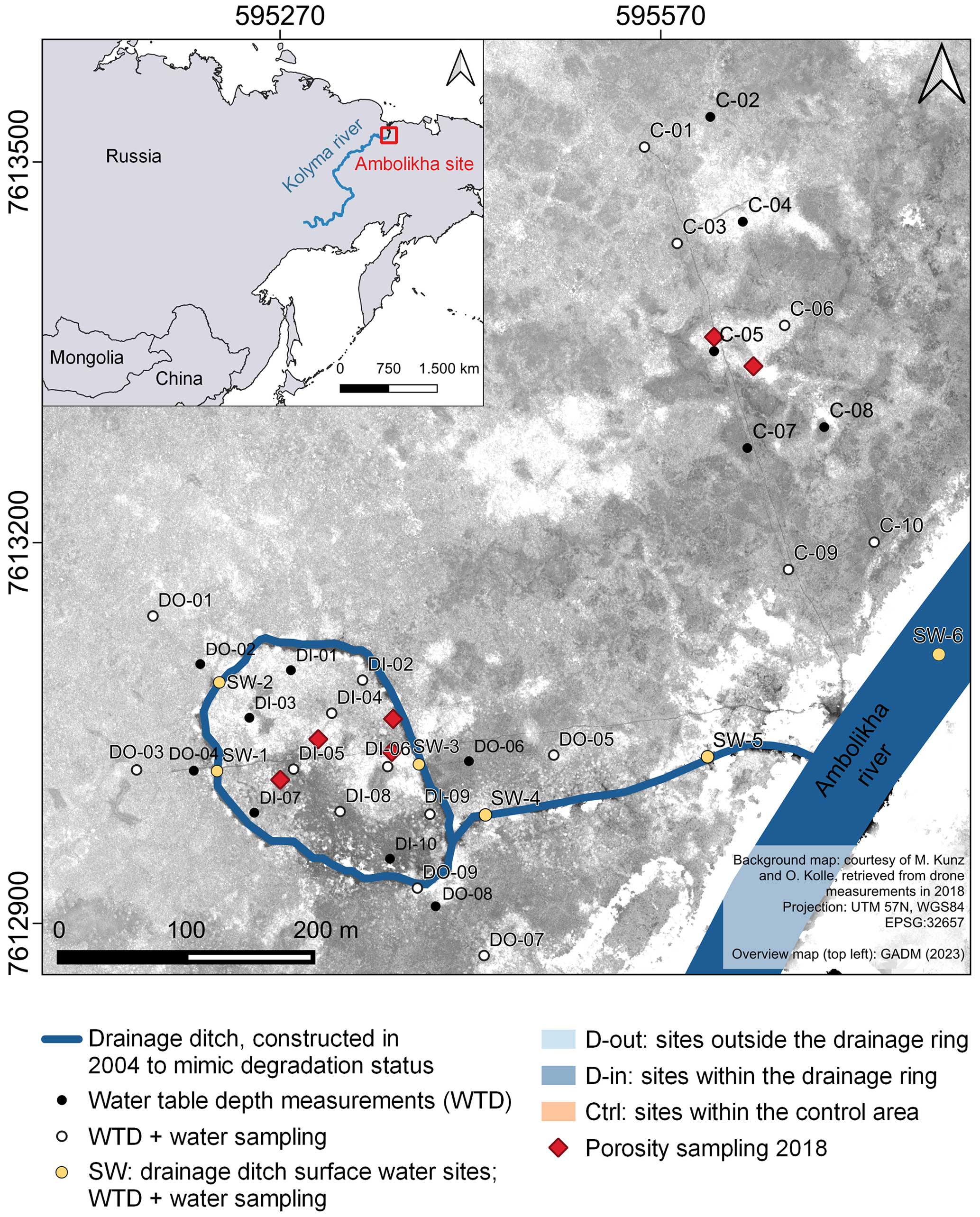
Figure 1Distribution of locations to monitor water level depth at the Ambolikha observation site. DI wells show piezometer locations at the drainage-inside (D-in) area, DO wells at the drainage-outside (D-out) area, and C wells at the control area (Ctrl). For this study, out of the six surface water sampling sites (marked in yellow) only at three locations within the drainage ring (SW-1 to SW-3) water levels were measured, and sampling was conducted. The black points show automatic water level measurement locations, and the white points indicate water sampling at several of these locations. The red diamonds indicate soil sampling locations for porosity analysis.
In order to determine the absolute water level above sea level, we obtained the elevation of each of the monitoring locations across the Ambolikha site based on a 2018 drone survey that produced high-resolution digital elevation maps (Fig. A5) of the surface and top of the piezometer pipes with a precision of ± 6 cm. The level of the ultrasonic sensor within the pipe and the soil surface adjacent to it were measured manually to account for different exposure heights of the piezometers. Our piezometers protrude ca. 78 cm (± 10 cm) from the soil. Based on this information, we were able to calculate the network-wide spatiotemporal variation in groundwater heads above sea level (groundwater level = h), as well as the depth to water table from the surface (relative water table depth) for groundwater and surface water.
In order to visualize spatial water level trends on the basis of the piezometric data, we first applied cubic spline interpolation (QGIS.org, 2022) on all surface and groundwater levels for four dates throughout the measurement period (Fig. 5). Mid-monthly dates were used to provide an overview of water levels throughout the growing season. The main directions of water flow were illustrated using the tool “gradient vectors from surface” in QGIS (QGIS.org, 2022).
Suprapermafrost water flow (Qw in m3 s−1) between piezometers was calculated with Darcy's law and given in liters per day (L d−1):
where K is the saturated hydraulic conductivity (m s−1), A the cross-sectional flow area (m2) based on groundwater level above the permafrost, Δh the water level difference between piezometers (m), and Δx the lateral distance between piezometers (m).
2.2.2 Soil properties
The saturated hydraulic conductivity (K) was determined based on slug-injection tests, which were conducted on 29 July and 30 July 2016. K was calculated according to the description of Bouwer and Rice (1976), resulting in two different values: 2.5 × 10⁻⁵ m s−1 for the organic soil layer and 7.4 × 10⁻⁷ m s−1 for the mineral soil layer. Depending on the amount of water located in the layers, the effective hydraulic conductivity (weighted mean) was calculated from the contribution of each layer to the active cross-section and applied to the Darcy flow calculation.
The extent of the organic layer was measured on 8 July and 17 July 2018. This was done by drilling six small holes using an auger within both the drained and the control areas. The transition between the organic and mineral soil layers was visually detected and measured. At these locations, samples for soil porosity measurements were collected in core cutters with a volume of 100 cm3. The soil samples were transferred to an on-site laboratory and weighed twice: first after 2 d of water-saturated conditions. Subsequently, the soil samples were dried at 105 °C for 24 h and weighed again. The porosity was calculated using the relationship between water volume and soil weight under consideration of the volume of the core cutter:
where Vp is the pore volume (g cm−3), Vt is the total volume (g cm−3), and Vs is the solid volume (g cm−3) of the respective soil sample.
where Pt is the soil porosity (%) that was calculated from the ratio between Vp and Vt.
2.2.3 Thaw depth
Thaw depth was measured by inserting a metal rod into the soil until the ice layer was reached (no further movement possible) and noting the distance from the soil surface. Thaw depth was measured at most of the groundwater monitoring locations as well as at locations distributed over the study site; measurements were taken repeatedly during the growing season. For most of the groundwater monitoring locations, up to eight measurements of thaw depth were taken between 17 June and 4 September 2017.
2.2.4 Stable water isotopes
For analysis of stable water isotopes, samples were collected from precipitation, surface water, suprapermafrost groundwater, and the upper permafrost ice layer. Rainwater was collected after rain events during the sampling period. In total, 3 surface water measurement locations and 16 groundwater piezometer sites were sampled for this analysis, 5 of which are located within the control area, 5 within the drainage-outside area and 6 within the drainage-inside area (Fig. 1). A total of 14 samplings were conducted in the growing season between 25 June and 5 September 2017. During that time, precipitation was sampled eight times subsequent to precipitation events. The permafrost ice was sampled on two dates in 2018: 3 and 6 July. Generally, the temporal resolution in the middle of the growing season was good but decreased in mid-August and the middle to end of September. The inclusion of additional data from July to August 2016, July to October 2018, and May to July 2019 covered early and late growing season isotopic signatures and provided sufficient data for monthly means (Fig. 7). This additional data resulted from our on-site measurements in 2016 and 2018, on-site suprapermafrost groundwater measurements in 2019, and precipitation measurements in Chersky from 2018 and 2019. During all 14 water samplings, electrical conductivity, among other parameters, was measured with a YSI Professional Plus multiparameter instrument combined with the respective parameter sensors (YSI Inc., Yellow Springs, Ohio, USA).
Water samples were collected, filtered (0.7 µm GF/F Whatman®, VWR International GmbH, Darmstadt, Germany), and transferred to 1 mL glass vials without headspace and kept at 8 °C prior to analysis. Permafrost ice water was sampled by drilling boreholes to the uppermost part of the active layer and melted prior to filtering and measurement. All water samples were analyzed for hydrogen (δD) and 18-oxygen stable isotope composition (δ18O), with a Delta+ XL isotope ratio mass spectrometer (Finnigan MAT, Bremen, Germany) at the BGC-IsoLab of the Max Planck Institute for Biogeochemistry in Jena, Germany, using a TC/EA (thermal conversion elemental analyzer) technique. Isotopic compositions relative to the Vienna Standard Mean Ocean Water (VSMOW) and the Standard Light Antarctic Precipitation (SLAP) are expressed as δ values in per mill (Coplen, 1994). The BGC-IsoLab further used three internal standards (www-j1, BGP-j1, and RWB-J1), and analytical uncertainties are about < 1 ‰ for δD and 0.1 ‰ for δ18O (Gehre et al., 2004). We set up an end-member mixing analysis (EMMA) to detect if the isotopic signal was derived from precipitation or snowmelt (at the beginning of the season) or permafrost melt (at the end of the season) signal. Since permafrost and snowmelt showed similar heavy directions in isotopic compositions, we can distinguish them only by early and late season.
where source 1 (end-member 1) represents the stable water precipitation signal (n=7, δ18O = −15.3 ± 0.7 ‰, δD = −118.2 ± 4.4 ‰) and source 2 (end-member 2) the heavier signal of permafrost ice (n=2, δ18O = −22.8 ± 0.2 ‰, δD = −180.8 ± 2.6 ‰). The proportion of source 1 is given in percent.
Deuterium excess (D-excess) was calculated in order to assess kinetic fractionation processes (Dansgaard, 1964). These processes gave indications of evaporation and condensation processes occurring within the samples. Samples with a deuterium excess < 10 ‰ represented an evaporative signal (Dansgaard, 1964).
where δD and δ18O represent the stable water isotopic values per site and sampling time.
3.1 Water table depth and water levels
Water tables for each of the four groups of water types differed significantly (p values < , RStudio software, stats package, t.test function). For suprapermafrost groundwater, water tables were the highest for control site wells, followed by drainage-outside areas and drainage-inside areas (Fig. 2). After the recession of the early summer flood, surface and groundwater levels receded across all sites. While most of the locations still showed inundation in June, these relatively wet conditions were followed by a decrease in water levels until the middle to end of July, most pronounced within the areas affected by the drainage. Accordingly, around the peak of the growing season in mid-July, most parts of the drainage area but also some locations within the control area (C-4 to C-6) had dry topsoil. After reaching the lowest water levels around early August, conditions remained relatively stable for the rest of the measurement period, followed by a minor to moderate increase linked to more frequent precipitation events and lower temperatures in September (see also Fig. 3).
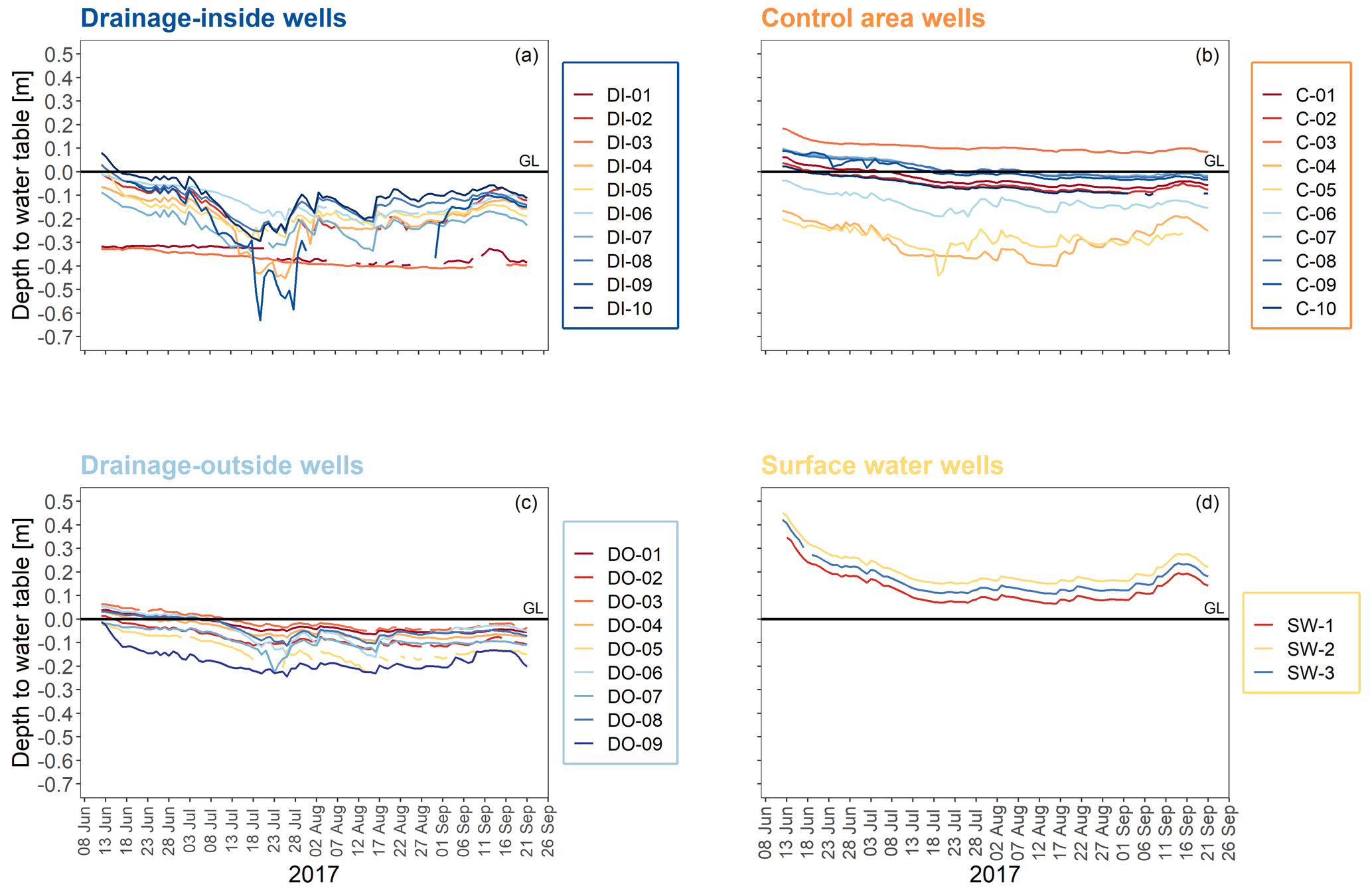
Figure 2Daily mean water table depth (water tables in relation to a ground level (GL) of 0 m, horizontal black line) in 2017 for all measurement locations. The individual panels show time series for each of the four hydrological sections (Table A1): (a) DI wells, (b) C wells, (c) DO wells, (d) SW wells. Values above the ground level indicate periods of waterlogged conditions. For the surface water locations, the ground level refers to the water–sediment interface.
Dry and wet locations reacted differently to precipitation: piezometric heads fluctuated during the course of the growing season. In general, all precipitation events were associated with an almost immediate increase in groundwater levels across sites. For example, most water levels at a predominantly wet site (C-01) for the entire observation period remained within a range of ± 6 cm, and daily fluctuations rarely exceeded 0.3 cm (Fig. 3). Strong precipitation events slowed down or even reversed the general drying trend over time, but observed increases in water levels usually happened slowly (over the course of several days). In contrast, at the drained site (for example DI-08, Fig. 3), we observed water tables as low as 30 cm below soil surface, and steep decline rates often exceeded 1 cm per day. There, strong precipitation events were followed by an instantaneous rise in water levels exceeding 5 cm several times during the observation period. Overall, the measured groundwater level range was about 3 times higher at drained sites compared to control sites.
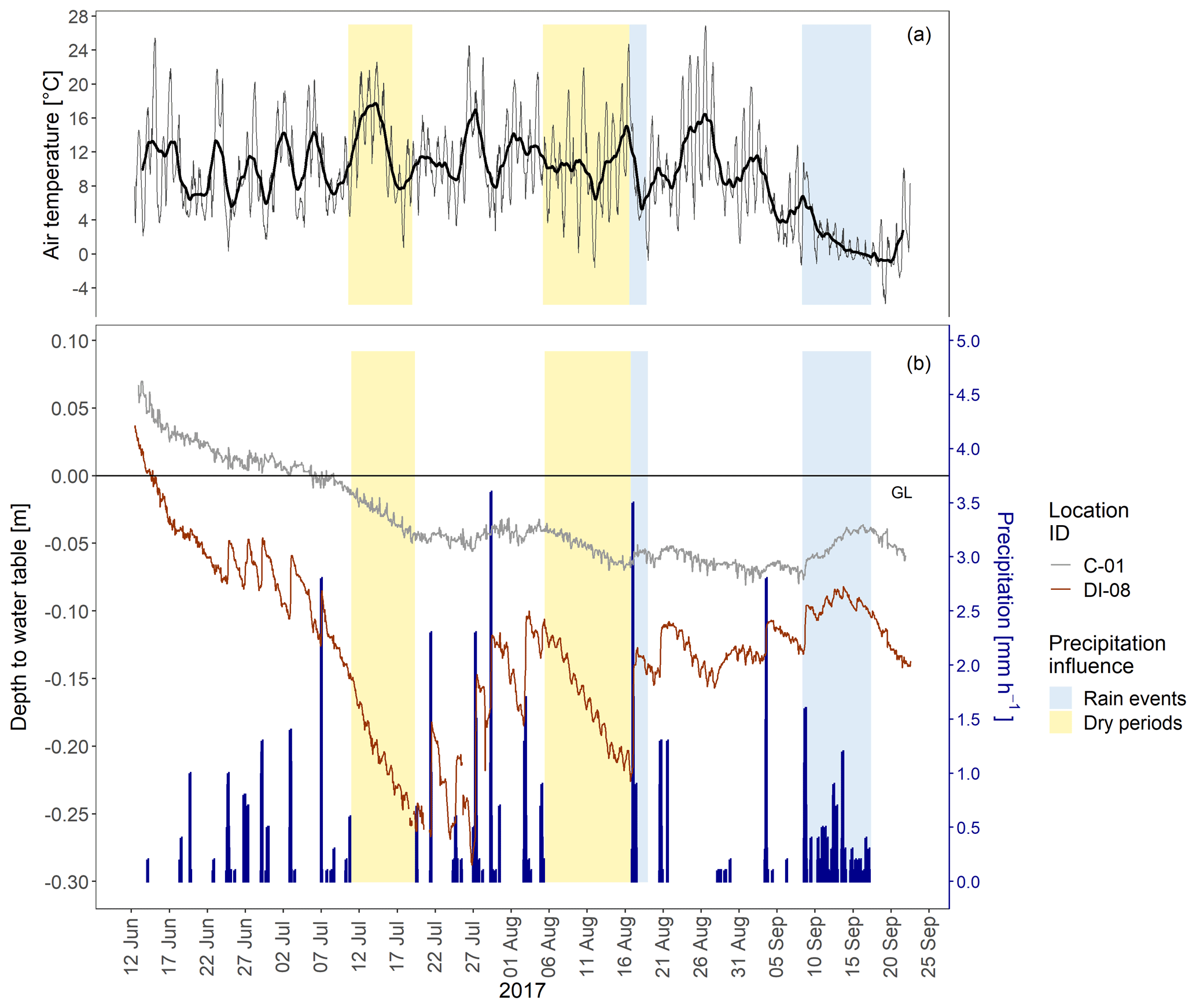
Figure 3Temperature, precipitation, and representative water tables over the course of the measurement period in 2017. Precipitation events are shown as vertical blue bars. The yellow shadings show representative dry periods (no precipitation for more than 1 week), and blue shadings show precipitation events. (a) Time series of the air temperature during the measurement period. The gray line shows hourly data; the black line shows the moving average (width of rolling window: 100 data points, zoo package, R Core Team, 2023) of temperature values. (b) Time series of precipitation events on two exemplary locations of groundwater levels. The red line gives water levels at a selected drained site (DI-08), while the gray line indicates conditions at a control site (C-01). In both cases, water levels are given as the depth from the ground level (GL; horizontal black line) to the water table.
We observed two representative dry periods in 2017, when precipitation was absent for more than 1 week: in July (from 10 July 2017 at 19:00:00 LT to 19 July 2017 at 12:00:00 LT) and in August (05 August 2017 at 07:00:00 LT to 16 August 2017 at 21:00:00 LT) (Fig. 3). Daily mean temperature during these dry periods rose to 18 °C in July but only 11 °C in August. Water level decrease rates differed distinctively between wells. For instance, the water level at C-01 decreased by 3.2 cm in July and 2.5 cm in August. In contrast, water levels at the drained site DI-08 decreased by 10.3 and 9.5 cm, respectively. A strong precipitation event at the same place on 17 August 2017 at 01:00:00 LT (3.5 mm h−1) increased water levels by 8.0 cm within 3 h after the start of the event. At C-01, the strong precipitation event resulted in only 1 cm water level increase with no or very limited lag time. Another strong precipitation event started on 8 September 2017 at 14:00:00 LT. During this 7 h event, C-01 and DI-08 showed similar increases in water levels (C-01: 3.9 and DI-08: 5.0 cm, Fig. 3), while, in contrast to the August event, the peak was delayed only at the control site C-01, not at the drained site DI-08.
Overall, daily groundwater levels were the highest in the morning (ca. 07:00:00–11:00:00 LT) and the lowest in the evening (ca. 19:00:00–23:00:00 LT), indicating evapotranspirative losses during the day. These fluctuations can be observed for all sites but were most pronounced at drainage-inside sites (Fig. A 4).
3.2 Water flow patterns
The highest piezometric levels at the control area were located in the north, whereas the lowest water levels were generally observed within the center of this section, indicating a potential lateral subsurface outlet (Fig. 4). Across the site, water levels tended to decline until August and then slightly recovered. Linked to this, the flow patterns showed a pronounced variability over the course of the growing season. In general, water from the wetter areas in the north and the south flowed towards a convergence zone in the center. The position of the central convergence zone shifted with time from the southern part (C-07, C-08) to the northern part until mid-August and then back again south until the end of the observation period. Accordingly, during high water levels, the main outlet for water from the study area is located close to C-08, whereas with lower water levels, water flows towards C-06 and drains down the surrounding floodplain.
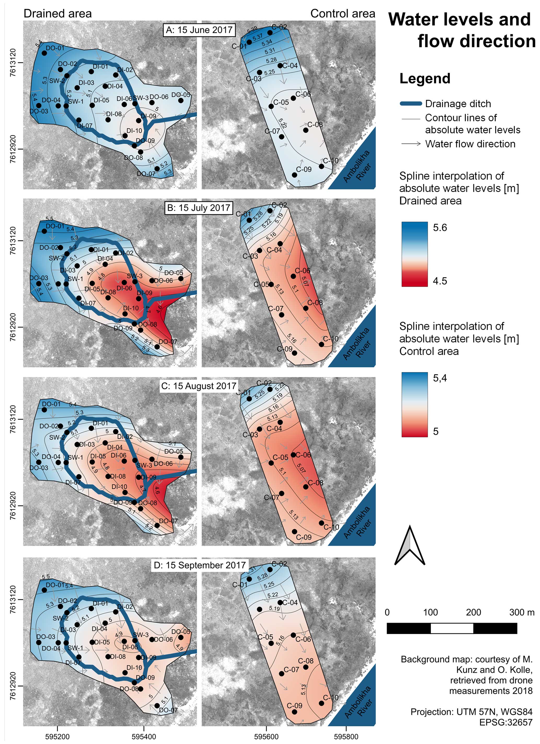
Figure 4Interpolated piezometric levels and flow directions for four selected dates (15 June, 15 July, 15 August, and 15 September) across the growing season in 2017 at the control and drained areas. Water level measurements in suprapermafrost water and surface water in the drainage ditch are shown with black dots. Flow directions are marked as arrows and contour lines of absolute water levels in gray lines. Interpolated water levels are indicated by the color code (low water levels in red, high water levels in blue); note the difference in color scale for the control and drained areas due to general differences in absolute heights.
Table 1Suprapermafrost Darcy flow velocities [L d−1] calculated for three time steps in 2017.
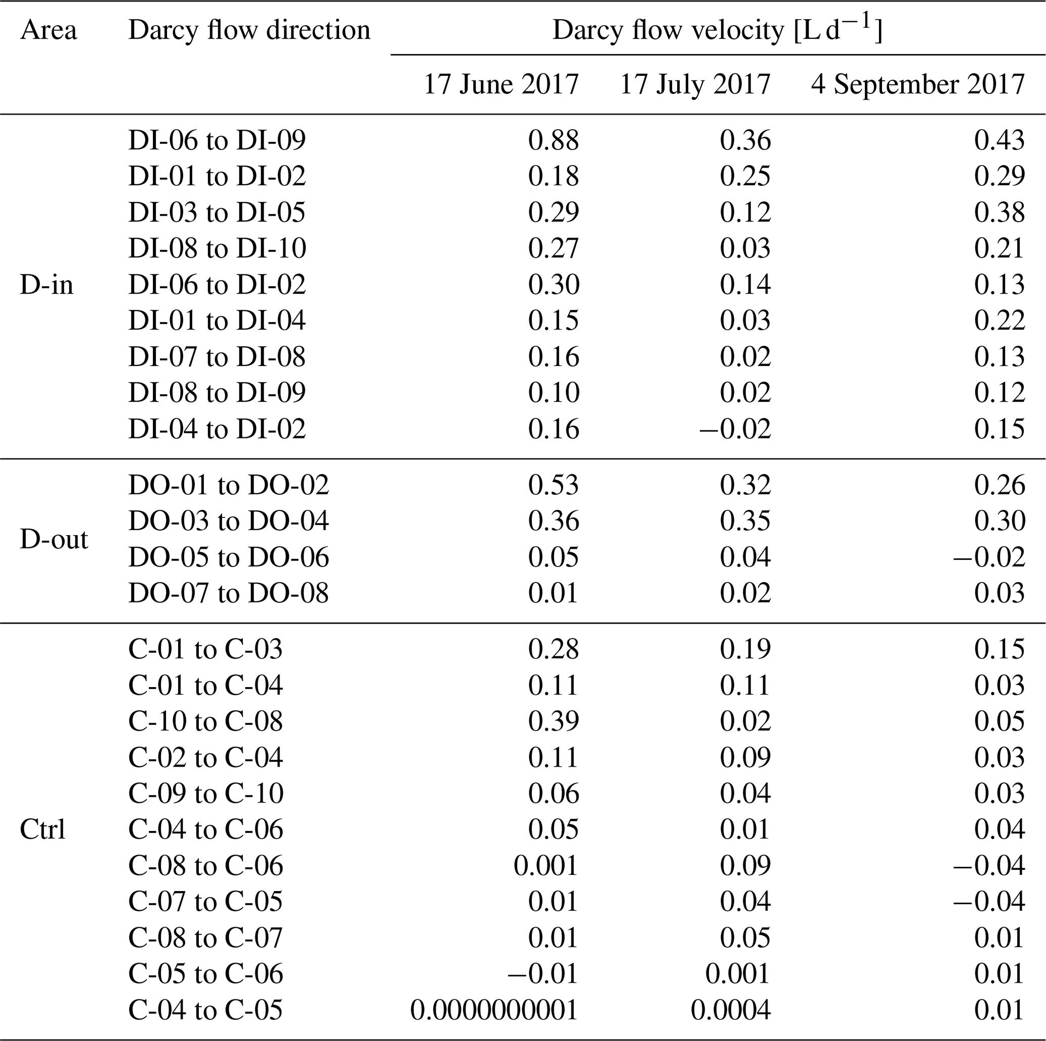
Within the drainage area, the spatial distribution of high and low piezometric levels maintained similar patterns throughout the measurement period: we observed the highest groundwater levels in the northwestern area and the lowest close to the outlet of the drainage ring in the southeastern part (Fig. 4). Locations inside the drainage ring showed the strongest temporal fluctuations, especially in the southeastern part where water levels were the lowest. Based on hydraulic groundwater gradients between sampling sites, we determined the expected main flow direction within the drainage ring to be oriented from northwest to southeast, e.g., groundwater flow towards the outlet drainage channel (especially towards SW-3, Fig. 4) and the Ambolikha River. The convergence zone was found in the southeast at the drainage ring area, around the connection to the outlet channel. During the drier months of July and August, lower water levels generally intensified the flow paths; however, the overall flow patterns within the drainage area remained stable over the course of the growing season, even though absolute water levels as well as their gradients within this treatment area changed over time.
The calculation of Darcy flow showed a relatively consistent pattern for drainage-inside areas. Darcy flows varied between reversed flow (−0.04 L d−1) between piezometer locations and a maximum of 0.88 L d−1. For many piezometer sites, high flow velocities were calculated for June, the lowest were calculated for July, and they were high again for September. Flow rates remained persistently high in some areas, whereas for the drainage-inside area in particular, the lowest flow gradients were found during mid-summer. Flow velocities within the control areas showed different patterns depending on the location of the piezometers (Table 1), including both permanent decline over the summer, as well as peak flow or low flow in mid-July. In general, the highest water flows were calculated for drainage-outside and drainage-inside sites followed by the control area.
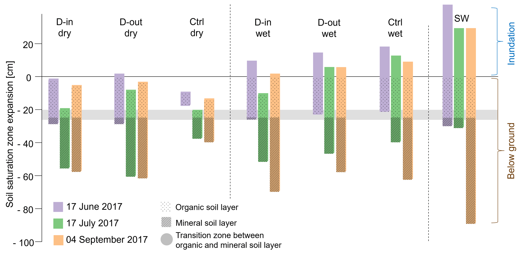
Figure 5Water saturation zones for three measurement times (17 June, 17 July, and 4 September 2017), for different water types (D-in, D-out, Ctrl, SW) and differentiated between wet and dry areas. The gray area represents the transition zone from the upper organic to lower mineral soil layer (D-in dry n=6, D-out dry n=1, Ctrl dry n=2, D-in wet n=4, D-out wet n=8, Ctrl wet n=8, SW n=3; see Table A1). Water saturation zones were calculated using water table as the top hydraulic boundary and ice table (based on thaw depth data) as the bottom boundary.
3.3 Soil water saturation
Thaw depths (Fig. 5) showed an initial steep decline at dry sites but had stabilized by late summer (49.0 ± 12.4 cm on 4 September 2017). In contrast, wet sites were characterized by a lower initial decline in thaw depth, but continuously deepening thaw levels ultimately bottomed out in September (62.7 ± 8.0 cm).
Water levels declined continuously only at wet sites of the control area. For all others, there was a minimum water level in mid-summer, followed by an increase. This progression was emphasized in the drained-inside area (dry and wet), where the initial drop in water levels was steepest. Water levels recovered slightly in September, when most of the control area water levels continued declining (Fig. 5). In the vertical structure of the soil profile, a transition zone (20–26 cm belowground) separated the upper organic layer from the lower mineral soil layer. The pronounced difference in mean porosity (Table A4) observed between the organic layer (79.0 ± 3.6 %) and the mineral soil layer (24.1 ± 2.0 %) had an effect on the extent and temporal dynamics of the saturation zones. Data from mid-June, mid-July, and early September revealed differences in the overall locations as well as the dimension of the saturation zones (Fig. 5). The extent of the saturation zone is generally the lowest in June. Shallow thaw depth tables in June corresponded to the extension of the saturation zone limited to the organic soil layer, although water levels were at their highest. In contrast to dry sites (Table A1), wet areas were inundated the most in June. The size of the saturation zone in July increased slightly for wet areas and substantially for dry areas and shifted downwards into the mineral soil layer. The largest extent of the saturation zone can be found in September, where the increase mainly resulted from water levels at the dry sites and from thaw depth at the wet sites. Generally, more extensive total saturation zones were found at wet sites (ca. 10 cm larger at the drained area and ca. 37 cm larger at control sites) in contrast to dry sites. Surface waters showed the highest water levels and a large increase in thaw depth in the late season.
3.4 Stable water isotopes
Data for water isotopes showed two main patterns: (a) temporal differences, indicating that the mean June samples were most depleted in δD and δ18O, and (b) spatial differences between the areas D-in, D-out, Ctrl, and SW. Spatial differences highlighted that, in the period from July to September, surface waters were less depleted, followed by drainage-outside areas, control area, and drained-inside areas, even though the differences between suprapermafrost groundwaters were relatively low (Fig. 6). Apart from the June data and in most areas, the strongest depletion was observed in August, whereas in the drainage-inside area this peak was reached in July. The lowest range was found for drainage-inside locations; the largest shift occurred among surface water isotopes between June and July.
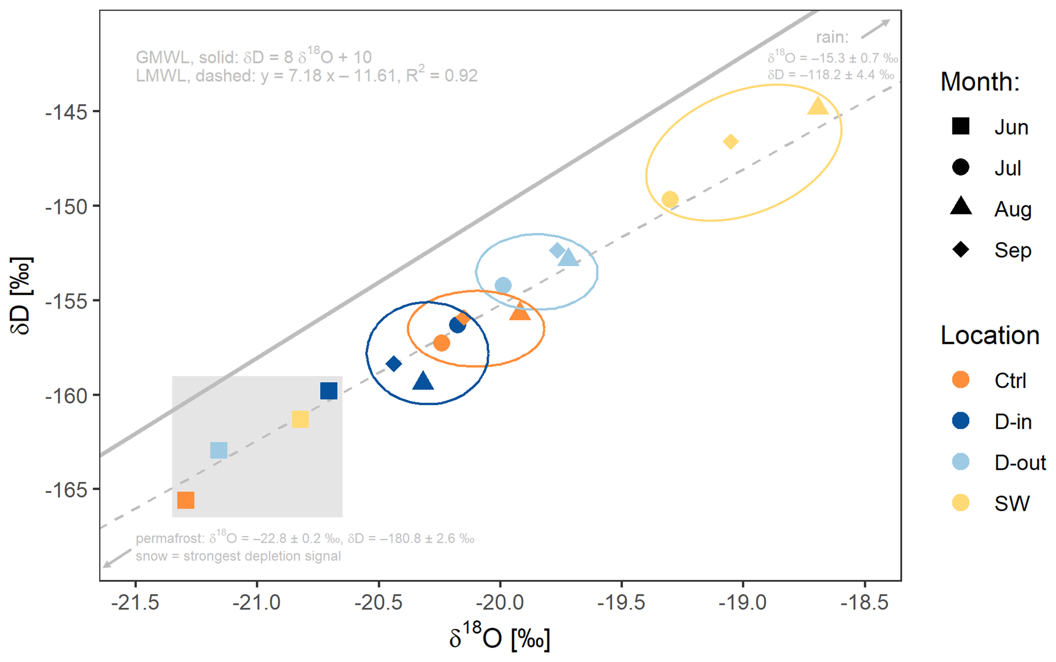
Figure 6Mean stable surface water and suprapermafrost groundwater isotopes measured from 2016 to 2019. The colors show the location of different water types; the shapes represent the monthly data. The circles in the respective colors visually summarize the months (July–September). The gray-shaded rectangle shows all of June's samples. The solid line represents the global meteoric water line (GMWL; δD = 8 × δ18O + 10) and the dashed line the local meteoric water line (LMWL; y=7.18 × −11.61; R2=0.92, own measurements).
The end-member values (Eq. 4) for permafrost ice (δ18O = −22.8 ± 0.2 ‰, δD = −180.8 ± 2.6 ‰) and for rain (δ18O = −15.3 ± 0.7 ‰, δD = −118.2 ± 4.4 ‰) used to calculate the local meteoric water line (LMWL) agreed closely with the values reported by Welp et al. (2005). Permafrost ice data were also in line with stable water isotopes analyzed by Opel et al. (2011), who investigated radiocarbon in Siberian ice wedges. Linking water isotopes with radiocarbon data, we can assume that our permafrost ice was formed in the Holocene (Little Ice Age). The average composition of the sampled water in the system was 42 ± 8 % of precipitation during the growing season and 58 ± 9 % snow (spring samples) and permafrost meltwater (late summer and autumn samples, Fig. 7). Over time, surface waters generally indicated decreasing snowmelt water signals and simultaneously increasing rainwater signals. A similar trend with continuously rising contributions from precipitation water over time was found at the wet locations DO-01, DO-07, and DO-03 at the drainage-outside area and C-01, C-03, and C-10 within the control area. In contrast, most of the drainage-inside sites, and also dry to intermediate sites in other areas (such as DO-09, DO-05, and C-06), initially showed a decrease in snowmelt water signal, followed by a substantial increase in permafrost water towards the end of the sampling period.
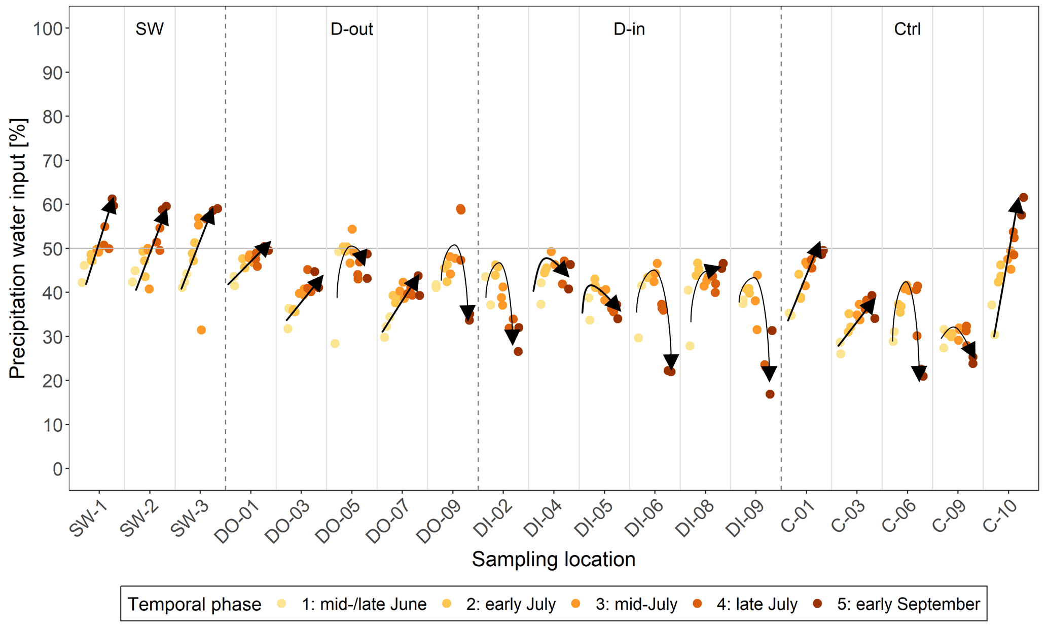
Figure 7Percentage of precipitation input (end-member mixing analysis) for δD of the samples during the measurement period in 2017. The lower the percentage, the higher the influence of stable water isotope signals; measurements are from snowmelt water in the early season (spring freshet) and from late-season permafrost meltwater.
Artificial drainage at the study site results in changes in hydrological conditions that contrast to those in a nearby control area; such changes affected water table depth, water flow velocity, and transport patterns. These shifts in surface and soil water regimes have secondary disturbance impacts on other ecosystem characteristics, including thaw depth and vegetation communities. How long water remains in a place (residence time) and the saturation status of soil water may constitute important factors driving the lateral mobilization of carbon in this site.
4.1 Degree of lateral connectivity impacts fluctuations in water levels
The contrasting water levels between the area inside the drainage (where water tables are low) and the control area (where water tables are high) led to different responses to precipitation events. As a result of the generally high water levels, water table trends at wet sites were smooth, and the influence of short-term precipitation was less than at dry sites. After four precipitation events (Table A3), the overall median water level increase was 0.049 m for drainage-inside areas, 0.01 m for control areas, and 0.018 and 0.022 m for drainage-outside areas and surface waters, respectively, highlighting the influence of precipitation events on drainage-inside areas. The accumulation of precipitation events had a long-term influence (Fig. 3), increasing water levels at all sites, but this signal was delayed. The increased lag time was a result of the laterally connected wet regions at the control area. Because of lower water levels above the frozen ground layer at the drained area, water levels were not as laterally connected as at the control area, and the increase in water levels was more than 3 times greater for short-term precipitation events during the driest temporal periods. The capacity of rainwater to infiltrate dry soils was faster than the lateral discharge towards the drainage ditch (Frampton and Destouni, 2015). During long-term precipitation events (such as those that occurred in mid-September, Fig. 3), this effect was minimized by generally higher water levels, a larger saturated zone, and increased lateral connectivity. The soil water capacity was reached at wet sites with water-saturated soils or inundated areas; there the rainwater flowed in the upper part of the organic layer and surficially. Water, which was redistributed over the area, moved slowly towards small channels and topographically lower areas, discharging into the Ambolikha River. During periods without rainfall, high evaporation rates, combined with an increase in air temperatures, led to low water levels. During this time, the potential for groundwater recharge was limited; water flow following hydraulic gradients (Walvoord and Kurylyk, 2016) was the main process affecting the water table depth. In general, precipitation input dominated temperature fluctuations; temperatures often dropped when rain fell (Fig. 3).
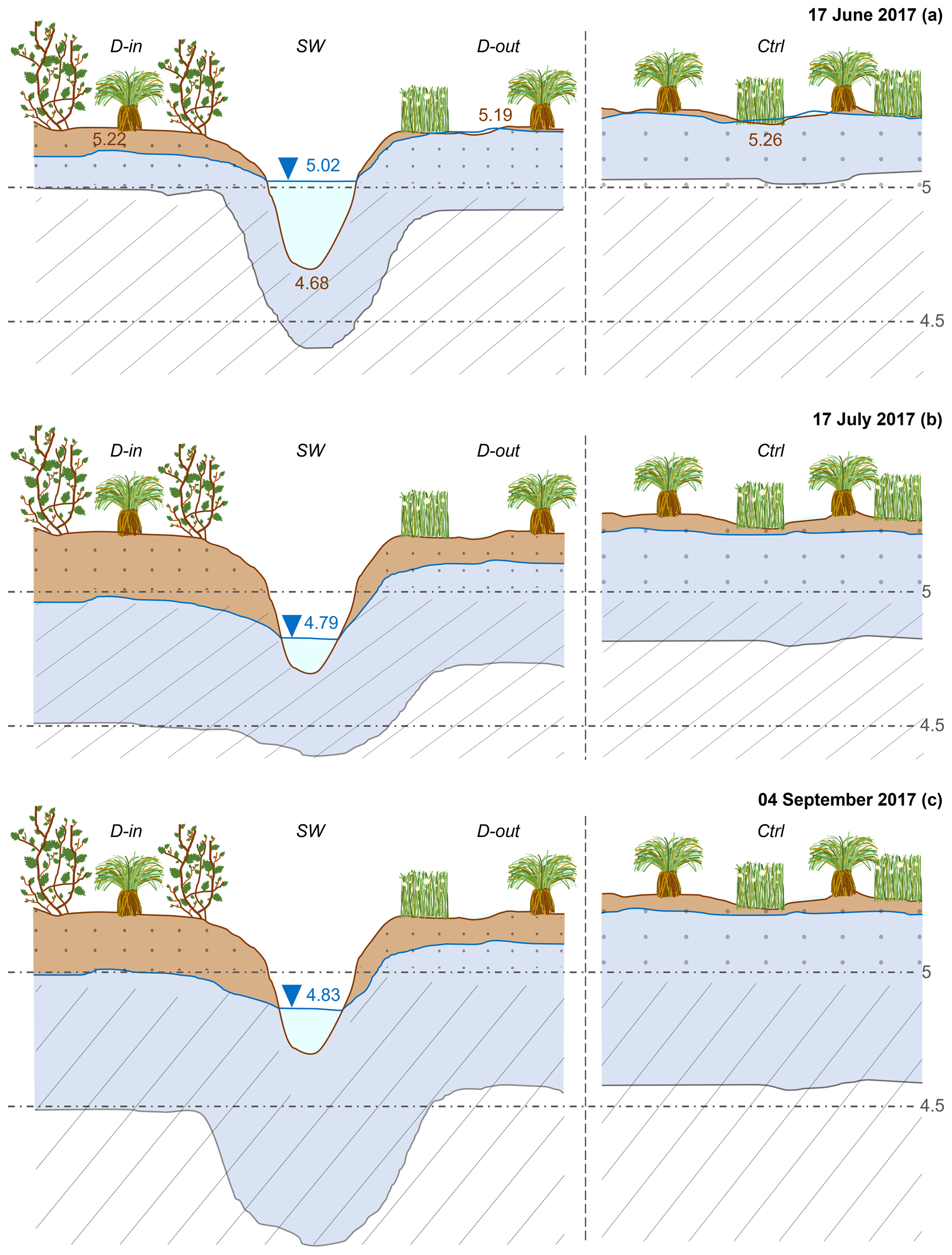
Figure 8Schematic water levels and thaw depth for three measurement times (17 June, 17 July, 4 September 2017; data in meters). From left to right the schematic shows drainage-inside (D-in), surface water (SW), drainage-outside (D-out), and control (Ctrl) areas.
Water levels and flow patterns followed a characteristic area-specific structure (Figs. 2–4, 8) according to which hydraulic gradients as well as soil saturation seemed to be the main drivers (O'Connor et al., 2019), although precipitation plays a short-term important role, except for consistent precipitation periods (e.g., September 2017). The more the soil area was saturated, particularly in the organic layer, the greater was the potential for lateral connectivity throughout the area. During the spring freshet in June, water flow was limited to the organic soil layer due to the shallow thaw depth (Fig. 8); permafrost represents an impermeable barrier (Grannas et al., 2013; Vonk et al., 2015). Surface water flow, inundation at wet sites, and groundwater discharge within the organic layer played a major role during this period (Woo and Young, 2006). At dry sites, transport was limited to the organic soil layer; there, without inundation water flowed less vertically connected in the soil column (Koch et al., 2013).
From early to mid-July, the spring freshet fully receded. Individual flow patterns appeared, and overall the lateral connectivity of water decreased (Fig. 3). A vertical soil water exchange at the drained area was inhibited by the very low water levels located mainly at the less permeable mineral layer. During this time water flow was lower and mainly located at the transition zone between the organic and mineral soil layer. Here, residence times relatively increased and water redistribution slowed down (Table 1). Infiltrated precipitation water could be accumulated at this transition zone and quickly discharged laterally before fully percolating into the mineral layer (Koch et al., 2014; Walvoord and Kurylyk, 2016; Wright et al., 2009).
In September, the vertical and horizontal water connectivity at drained sites increased when precipitation increased, and the input water was redistributed in both the organic and the deeper mineral layers (Fig. 8). Groundwater recharge through percolated precipitation was more prominent during that period, enhanced also by lower air temperatures and therefore less evaporation (Fig. 3). Moreover, limited photosynthetic activity at the end of the growing season limited water uptake. At control sites, connectivity remained high both laterally and vertically (in the organic layer, inundated water flowed on top, and the mineral soil layer provided strong input), even though inundation generally decreased over the growing season.
4.2 Water flow depends on micro-topography and the position of the water table in the soil column
Water flow direction and speed depended on several parameters: the amount of available water (mainly from inundation and precipitation), topography, and the location of the water table within the soil (Gao et al., 2018). The organic layer, characterized by high pore volume and high hydraulic conductivity, promoted water flow, in contrast to the mineral layer (Walvoord and Kurylyk, 2016). The lateral redistribution of water within this site therefore depended strongly on water table depth and thaw depth, determining the position of the soil saturation zone.
Microtopographic features, which led to a formation of local elevations and depressions at both experimental and control areas, profoundly impacted the small-scale redistribution of water. Measurement and sampling sites situated at local elevations (e.g., DI-03, DI-01, C-04, C-05) had relatively dry soils, whereas sites within local depressions (e.g., DI-10, DO-08, C-03, C-07) had wetter soil conditions throughout the study period. Soil composition at local depressions also differed from that at local elevations. High elevated sections were characterized by a large acrotelm layer (O'Connor et al., 2019); this uppermost organic layer comprised actively decomposed, highly permeable material and an overall thin organic layer. In contrast, low elevated sections had a large catotelm layer, comprising dense peat formation with low permeability (O'Connor et al., 2019). In this study, locating the transition zone between the organic and mineral soil layer was sufficient to explain major patterns in water flow velocity and hydraulic conductivity: high hydraulic conductivity within the organic soil layer sped up the flow of water into the nearby drainage ditch (Hinzman et al., 1991; Quinton and Marsh, 1998), especially during the spring freshet, when water levels were mainly located within this layer. Water flowed more slowly at control areas, possibly because of the thick catotelm layer. In contrast, the thick acrotelm layers of local dry elevations as well as the drained areas may have enhanced flow paths, allowing flow speeds to increase (Table 1).
The main water flow followed the hydraulic gradient from high to low areas correspondingly to topographical features (Walvoord and Kurylyk, 2016). This gradient was intensified at the drained area by the construction of the drainage channel. There, water was first directed to the discharge areas, then to the outlet of the drainage ring, before discharging into the Ambolikha River. Such a lateral surface connection in a channeled flow underlies degraded polygonal tundra systems (Liljedahl et al., 2016; Serreze et al., 2000); the installation of the drainage system at the site is intended to reproduce these degraded systems (Göckede et al., 2017; Merbold et al., 2009). Inside the drainage ring, the main flow direction followed the gradient from higher to lower elevated areas, with water mainly entering the drainage channel around site DI-09 (and DI-10, SW-3). This site, which was the closest to the drainage ring outlet, was characterized by a very low general water table and potentially low water residence times (Koch et al., 2013). Most of the suprapermafrost water with its constituents left the inner drainage system at this site and transitioned into surface waters. The autochthonous carbon at the drainage channel was then further transformed (assimilated by microorganisms and oxidized), before being transported within the drainage channel.
The calculated suprapermafrost water flow at drained sites, where water followed hydraulic gradients, was faster in June and September compared to at the control area (Table 1). In July, when water levels decreased to the minimum measured during the season, water flow was limited to the less permeable mineral layer, and the water column within the soil was the smallest. During that time, discharge into the drainage channel decreased and was influenced by short-term precipitation events although the flow direction remained the same. Likewise, the convergence of flow within the drainage area around site DI-09 was much more intense during summer months (July and August) (Fig. 4).
The main flow direction at the control area was from the north and towards the Ambolikha River, which represented the overall hydraulic gradient; however, a small dry ridge was identified in the area (C-04, C-05, and C-06). South of this ridge, the water flow direction in June and September was sideways and followed small belowground flow paths characterized by slow water flow speeds and therefore higher residence times compared to those at drainage sites. During the lowest flow in July and August, lateral water export shifted northward (Fig. 4), probably due to small impediments at the site and roughness in soil texture. This also led to changes in ephemeral small belowground drainage channels (Connon et al., 2014). Seasonal shifts in preferential flow paths may have changed the extent of carbon concentration (e.g., how much previously accumulated carbon was transported). Most of the wet areas could be associated with local depressions and confluence sites, where groundwater accumulated from the surrounding area and was slowly laterally exported (Connon et al., 2014). Location C-10, which was directly affected by the Ambolikha River, discharged towards the river throughout the measurement period.
Permanent inundation and very wet soil conditions led to a saturated organic layer over the growing season; slow water movement and relatively long residence times were observed, as they were at the control area, where the water flow was generally the lowest (Table 1). Such long residence times may be associated with large vertical flow paths because percolation is pronounced when the active layer deepens (Frampton and Destouni, 2015; Koch et al., 2013). Carbon production (anaerobic vs. aerobic) may be influenced in turn, as may carbon export (e.g., direct vertical release from inundated water column, Dabrowski et al., 2020; Wang et al., 2022).
Most sites dried completely from June to July due to decreased freshet water, increased air temperatures, and lack of rainfall. Although thaw depth increased, the organic layer became very dry, and the remaining porewater in the mineral layer was at its lowest at dry and drainage sites (Fig. 5). Porosity within the mineral layer was more than 3 times lower compared to within the organic layer (Table A4). With the gain in water experienced by drainage-inside areas in both soil layers between July and September, carbon could be exported through the system. At control wet sites, water gain within the mineral zone could be detected, but at the same time, water loss in surficial water was observed.
The abundance of stable water isotopes measured in this study indicated the seasonal composition and transition of the surface water and groundwater influenced by evaporation and the presence of snow and precipitation events and helped identify pathways for lateral water transport at both study sites. The temporal trend at drained sites showed a clear shift from a snowmelt-dominated signal at the beginning of the study (i.e., more depleted δ18O and δD values) that decreased over time and was replaced by permafrost thaw signal at the end of the measurement period. Control sites, which were influenced the most by precipitation signals, accumulated water flow throughout the area.
In July, the composition of stable isotopes indicated an increase in the relative contribution of the rainwater signal (Ala-aho et al., 2018). Towards the end of the measurements (August and September), the patterns between the control and drained areas became distinctive. At sites that were well connected vertically and laterally, with high to inundated water levels, rainwater dominated. Moreover, the composition of stable isotopes was less depleted and more in contact with the surface at control areas and therefore more prone to evaporation (Welp et al., 2005). Most data showed a deuterium excess of < 10 ‰ (Fig. A3), which was attributed to an evaporative fractionation signal and enriched precipitation in summer (Ala-aho et al., 2018). The hinterland component for control areas and drainage-outside areas was an important source for water input in this context, slowly supplying water from adjacent connected areas (O'Connor et al., 2019). Therefore, the relative location of a site within a larger area with multiple topographic features is pivotal for water accumulation or discharge. The initial increase in stable water isotopic composition at the drained sites had disappeared at the end of the study period, signaling permafrost thaw (Figs. 6, 7). This decrease was attributed to early summer water sources (snowmelt and precipitation) having largely drained out. Furthermore, Ala-aho et al. (2018) highlighted that snowmelt water contributed much more to summertime water flow than expected. This contribution is possible when water that was initially replenished in local depressions interacted with suprapermafrost groundwater during the mid-July low-flow regimes (Ala-aho et al., 2018). Surface water isotope signals gradually increased and were the most influenced by precipitation. Including the full isotopic dataset from 2016 to 2019 in this study allowed for a more general view of monthly data variability. The largest difference in isotopic data was found for surface waters from June to July, indicating that in June, waters mainly consist of snowmelt, whereas in July, waters are dominated by precipitation (Fig. 6).
4.3 Drainage feedbacks on thaw depth dynamics
Small-scale variations in thaw depth influence the movement of active layers and exchange between surface water and suprapermafrost groundwater. Shifts in thermal conductivity and heat capacity affect permafrost by affecting subsurface water flow (Sjöberg et al., 2016; Walvoord and Kurylyk, 2016). Both factors influence the seasonal development of thaw depth in permafrost soils and are strongly determined by hydrologic conditions. In the beginning of the growing season, very wet soils have a high heat capacity, which initially impedes the deepening of the thaw layer. Starting by mid-July, the wetter microsites have lost enough standing water to considerably lower their heat capacity, whereas thermal conductivity is high so that thaw progresses into autumn (Fig. 5). Our observations demonstrate that drainage speeds up the initial drying of topsoil layers following flooding in early summer. As a consequence, the heat capacity of microsites affected by drainage is quickly diminished, and the thermal conductivity, which affects the progression of thaw, is enhanced. However, organic topsoil layers had already begun to dry out in June, and by mid-July, decreasing thermal conductivity had mostly slowed down the thawing process (Fig. 5). The energy that heats up the upper layers does not penetrate the deep layers due to low thermal conductivity, slowing down the thawing process. These effects were also shown in a previous study in the same study area (Kwon et al., 2016).
4.4 Drainage impacts on site characteristics and biogeochemical cycles
Vegetation adapted to high water levels, such as cotton grasses (Eriophorum angustifolium) and tussocks (Carex species), developed in the predominantly wet areas (Fig. A2) within the undisturbed floodplain (Kwon et al., 2016). The change in hydrologic status also shifted the main vegetation type towards shrubs and tussocks with shrubs dominating the drained area (Göckede et al., 2017; Kwon et al., 2016). Shrubbier vegetation was able to develop a deeper and larger root system when soils were drier. Drier, warmer topsoils generated by drainage promoted this change in vegetation. Such changes could alter the energy balance (snow cover, shading) and, combined with evaporation, lead to further changes in the annual hydrologic regime. Because these vegetation types require more water, the soil wetness remains reduced. With more water uptake, vegetation was also able to enhance evapotranspiration (Chapin et al., 2000; Merbold et al., 2009). This may further dry out soils and promote vegetation with a deeper rooting zone, reinforcing and confirming the change towards drier soil conditions and an enhanced channeled flow (Liljedahl et al., 2016).
Overall, more water left the drained (inside and outside microsites) area, and the exchange with the organic soil layer varied over the growing season. The increased groundwater discharge towards surface waters was consistent with findings of many other studies (Connon et al., 2014; Déry et al., 2009; Evans and Ge, 2017; Frampton et al., 2013; Kurylyk et al., 2014; Lamontagne-Hallé et al., 2018; Walvoord and Striegl, 2007). Increased discharge leads to varying carbon production and transformation and transport towards surface waters (Walvoord and Striegl, 2007). Speeding up suprapermafrost discharge within the drainage area could lead to more rapid lateral transport of constituents towards surface waters (Walvoord and Kurylyk, 2016). We expected the faster water flow during and directly following the spring freshet (June) and higher precipitation inputs (September) to laterally transport high concentrations of dissolved organic carbon (DOC), and we assumed these concentrations would decrease towards the warmest time in summer (Guo et al., 2015; Prokushkin et al., 2009; Vonk et al., 2015). Therefore, the lowest DOC concentrations were expected during the low-flow period in July and August in 2017. During the driest period in July, water transport and leaching of carbon were limited to the mineral soil layer. Instead, there is a stronger focus on collecting permafrost thaw water within the mineral layer, but due to low hydraulic gradients and conductivity, exported water masses are relatively low. When low water tables create drier soils, the potential for microbial respiration increases, which in turn shifts CO2 production (Göckede et al., 2019; Kwon et al., 2019). Furthermore, the birch effect, which represents a quick release of CO2 due to soil rewetting (e.g., precipitation events), also leads to changes in carbon export in comparison to natural wet soil conditions (Singh et al., 2023). However, CH4 production in dry areas is much more reduced due to limited water saturation and anoxic conditions (Bastviken et al., 2008; Dabrowski et al., 2020). Shifted biogeochemical signals may therefore be caused by quicker discharge and drier soil conditions induced by permafrost degradation.
We investigated the response of permafrost ecosystems to the drier conditions expected as a consequence of climate warming. Our field experiment was based on an artificially constructed drainage ditch in an Arctic floodplain underlain by permafrost, which allowed us to study hydrological effects in a dry area compared to a nearby wet control area. This setup mimics landscape transitions due to permafrost degradation, including hydrological and vegetational changes.
In summary, this drainage resulted in lowered water tables, drier soil conditions, taller vegetation, and differences in flow dynamics and water isotopic signatures. An increase in hydraulic gradients caused by the drainage ditch sped up overall lateral water flow velocity, especially when water levels were located within the organic soil layer. When water levels dropped into the less permeable mineral soil layer, velocity slowed and vertical and lateral connectivity decreased substantially. The Darcy flows at the control area were much lower, which caused longer water residence times compared to the drained area. An expansion of drainage areas in these ecosystems can lead to shorter water residence times, which at the same time will affect the timescales of flushing of carbon and nutrients as well as transformation processes. This observation was also supported by changes in the isotopic composition of our water samples, which indicated that the contribution of different water sources (precipitation, permafrost melt, and snowmelt water) shifted between the drained and control areas. The shifts in vegetation structure induced by drainage may have significantly influenced the local carbon budget by altering carbon sinks and sources, as well as water balances, through related shifts in evapotranspiration.
In addition to permafrost degradation induced by global warming, other disturbances such as wildfires can also lead to subsidence and changes in hydrological conditions. Therefore, the findings from our field experiment may be relevant in any landscape subject to accelerated lateral water flow and associated constituent transfer, which may for example impact the location and speed of transformation processes that lead to the release of carbon dioxide and methane. It is necessary to further analyze the increased abundance of such degraded landscape patterns to better understand potential risks of infrastructure collapse and how this affects the progression of thaw slumps and thermo-erosion. The results from our study demonstrate adequate requirements to compare and characterize natural conditions with a drainage-influenced area regarding suprapermafrost water level shifts. Future studies should focus on combining lateral and vertical water and carbon fluxes to better understand how the carbon processes and transport pathways respond to projected shifts in hydrological dynamics in tundra ecosystems.
Table A1Water type description and wetness indicator throughout the measurement period for each location.
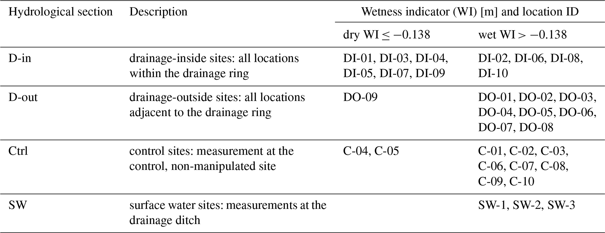
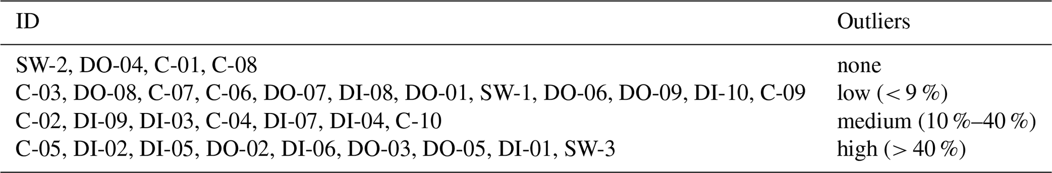
Table A3Four selected precipitation events throughout the measurement period.
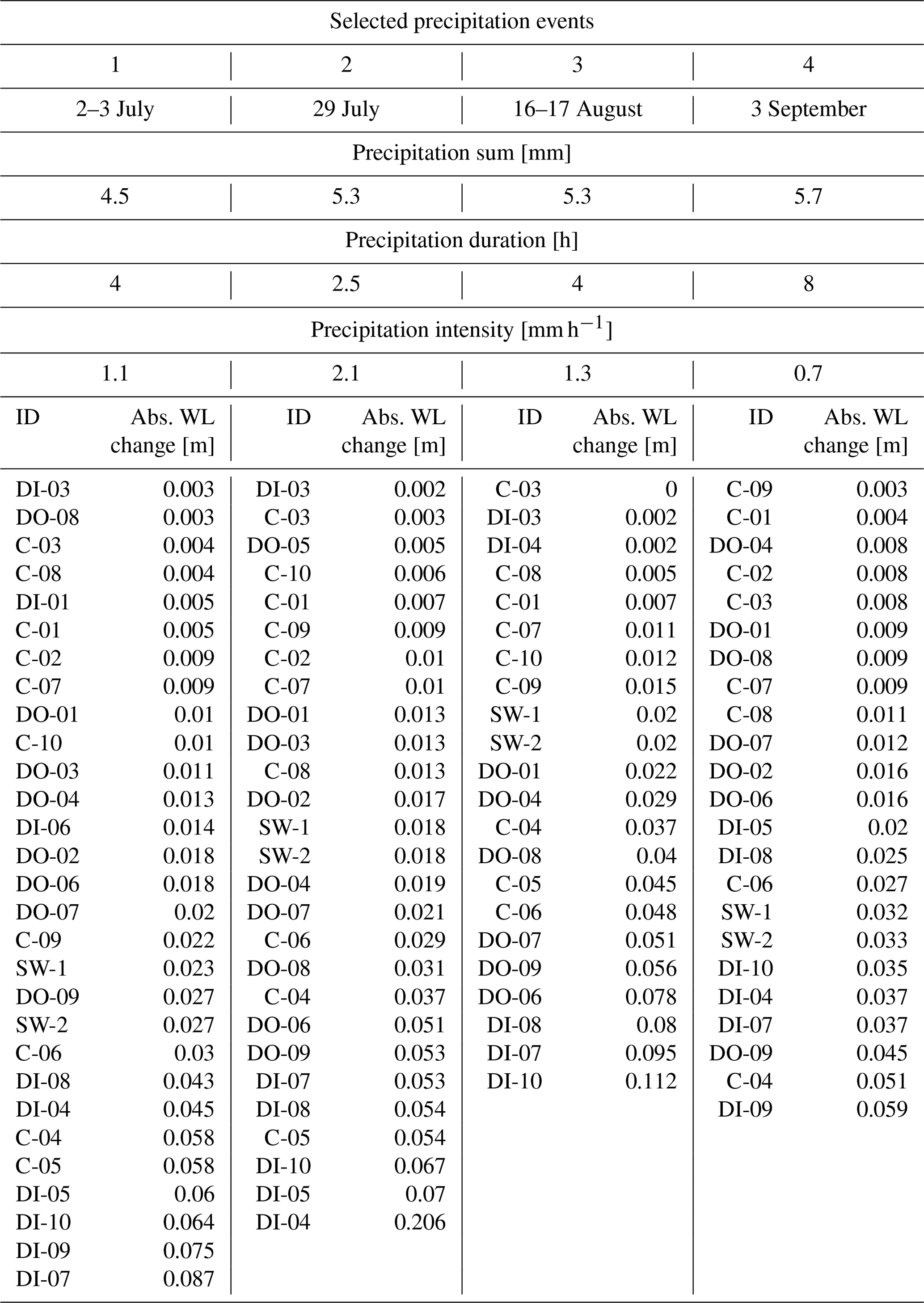
Table A4Porosity measurements in 2018. In six locations across the study site, samples from upper organic and lower mineral soil layers were analyzed for porosity (in total 14 samples – 7 from the organic layers and 7 from the mineral layers). The mean transition between the organic and mineral layers was 23 ± 3 cm belowground. Mean porosity values for organic material were 79 ± 4 % and for mineral material 24 ± 2 %.
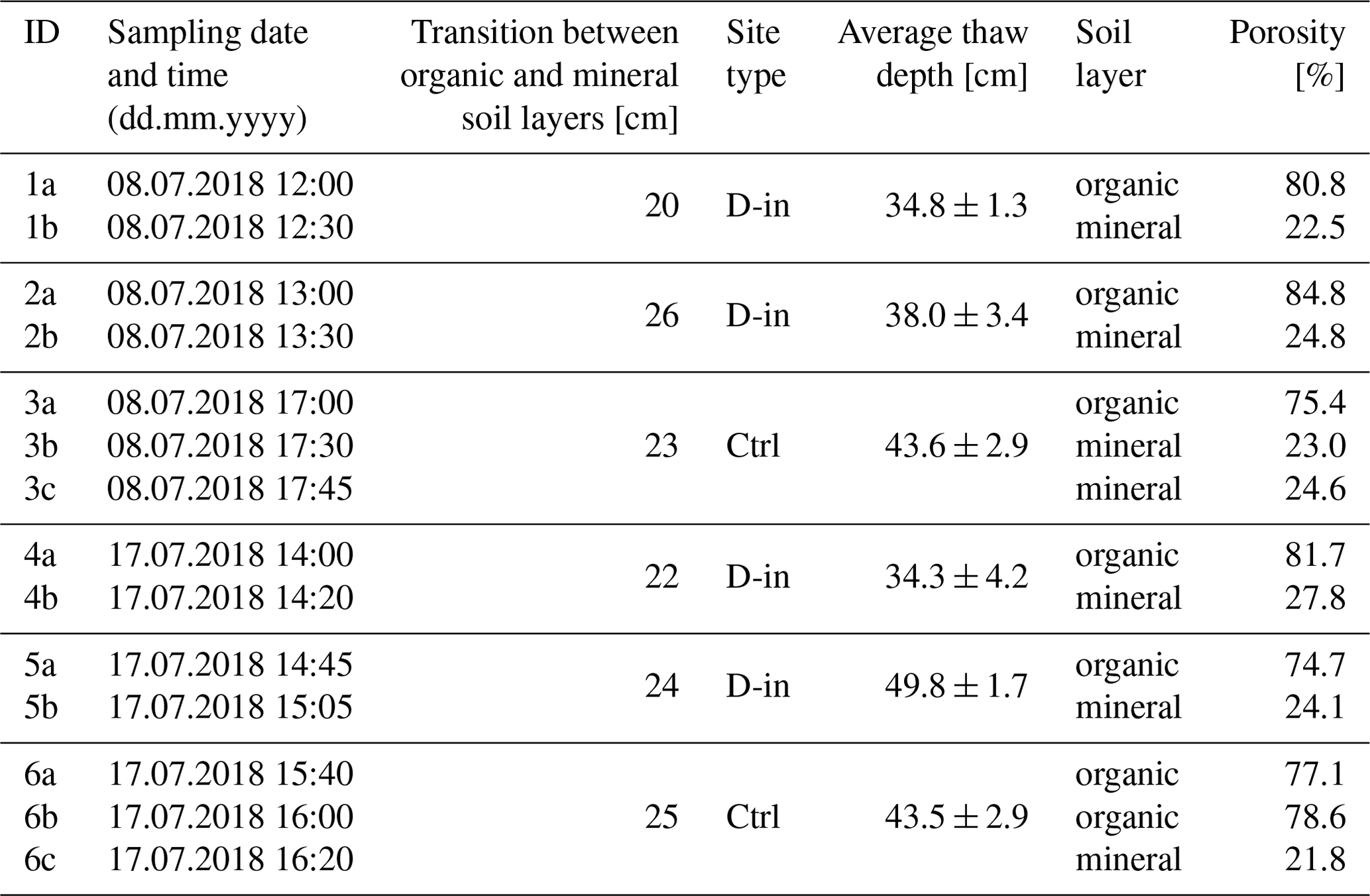
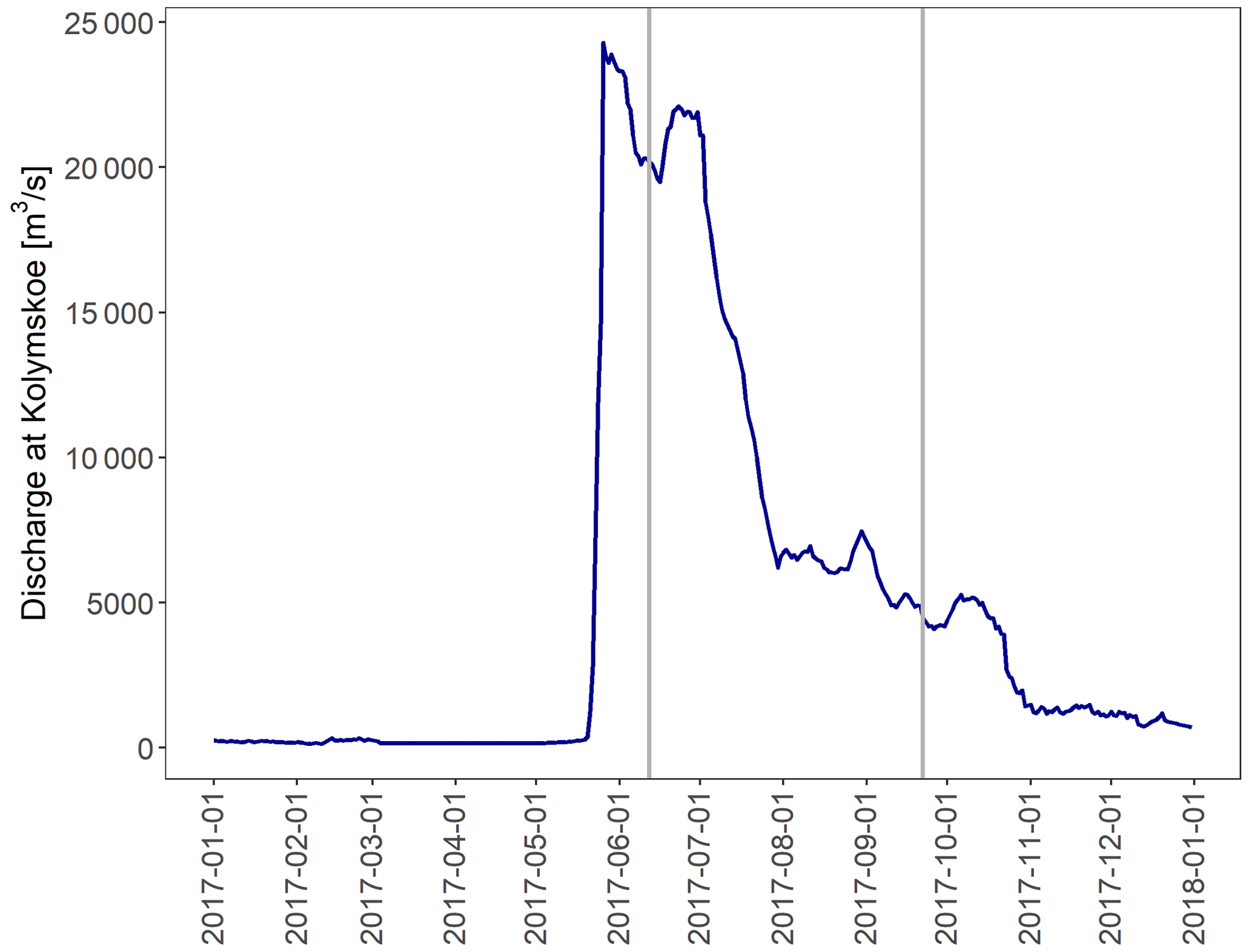
Figure A1Hydrograph at Kolyma station in Kolymskoe showing a nival streamflow regime. The first peak during spring freshet was between 26 May and 3 June 2017, the second peak was between 20 June and 1 July 2017, and the summer low flow was between 30 July to ca. 30 October 2017. The gray lines represent the start (12 June 2017) and end (22 September 2017) of the ultrasonic water level measurements. Data: McClelland et al. (2023).
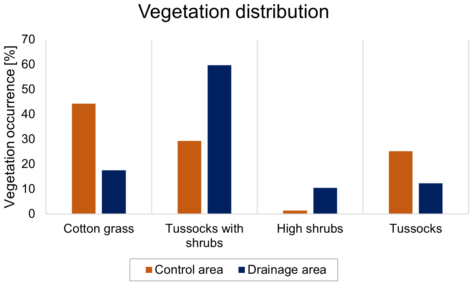
Figure A2Vegetation distribution over drained (blue) and control areas (orange). The predominant vegetation types at the drained (mainly dry) area are high shrubs and tussocks with shrubs. The predominant vegetation types at the control (mainly wet) area are cotton grass and tussocks.
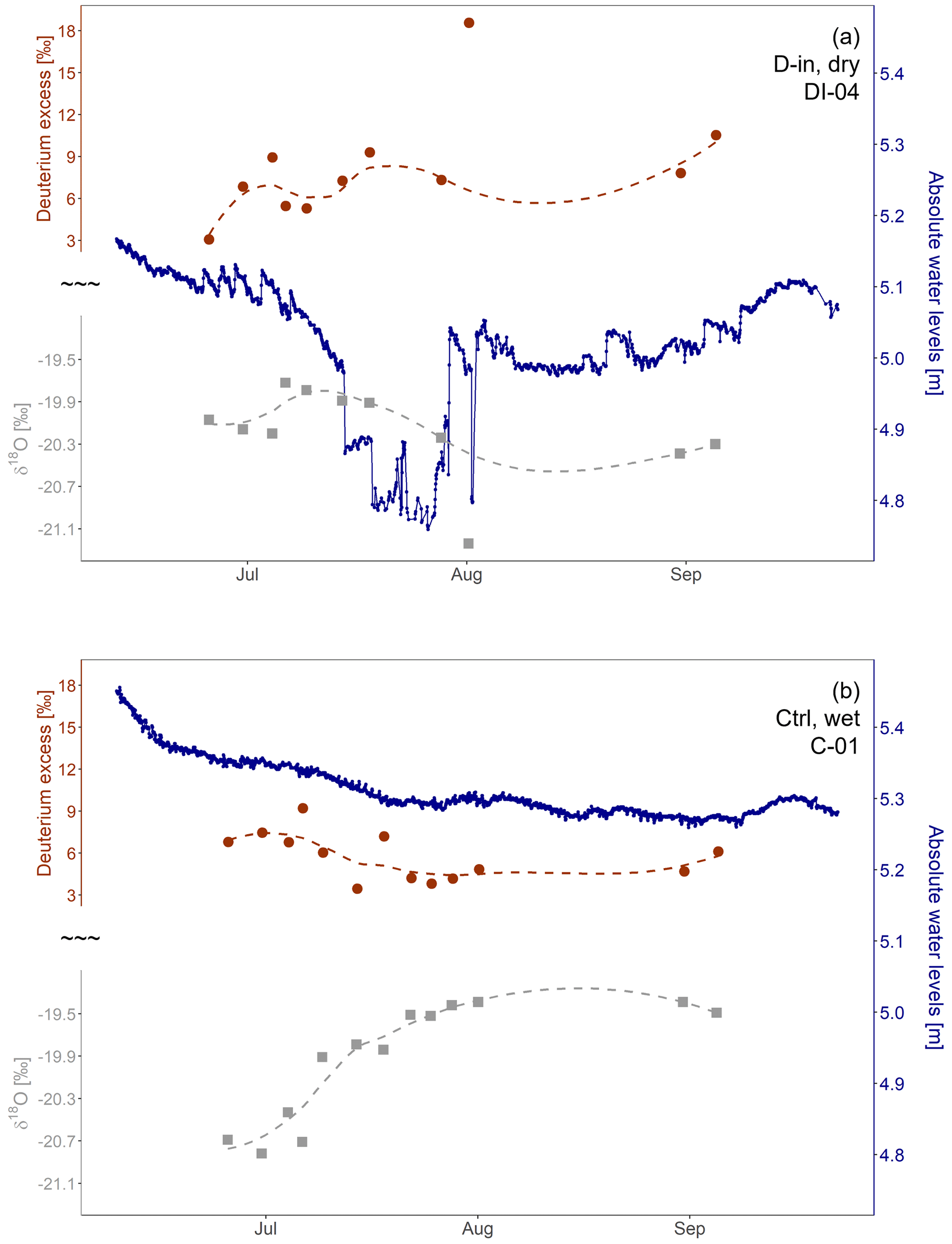
Figure A3Time series of the water levels (blue line) combined with δ18O data (gray points) and D-excess (red points) at a (a) dry location within the drainage ring (DI-04) and at a (b) wet location in the control area (C-01).
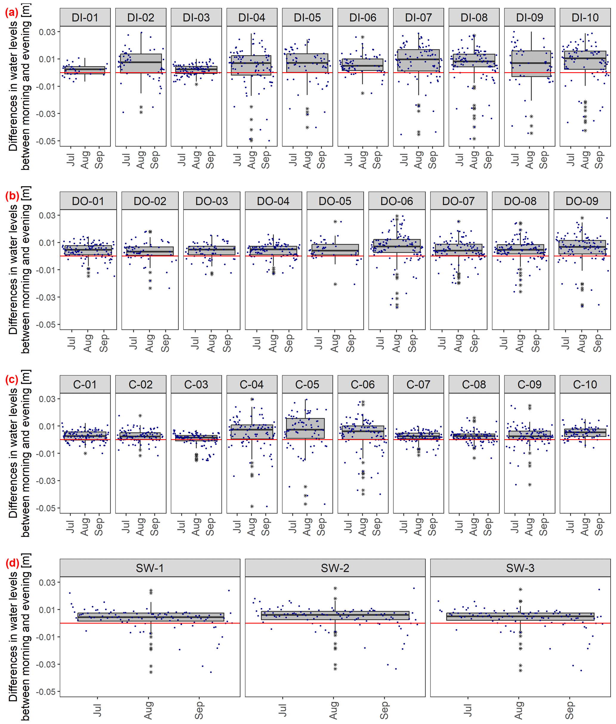
Figure A4Differences in water levels per day. Morning (07:00:00–11:00:00 LT) and evening (19:00:00–23:00:00 LT) mean values were calculated every day. Boxplots of the differences between these two time periods are shown for all measurement sites: (a) D-in, (b) D-out, (c) Ctrl, (d) SW sites. Vertical scales were truncated to enhance visibility and comparability; some outliers are not shown. The red line represents 0, and all data above 0 indicate that water levels were higher in the morning compared to the evening.
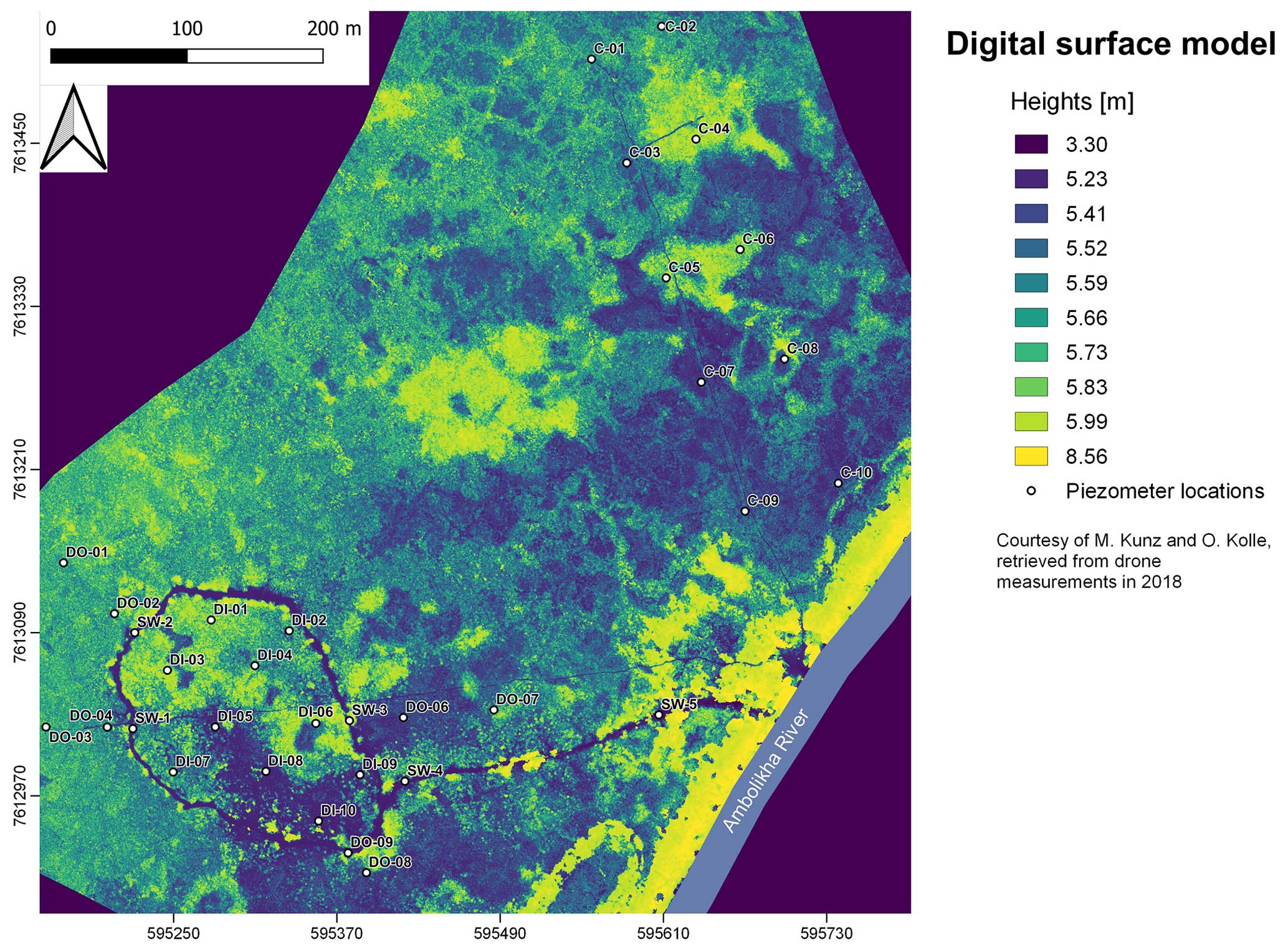
Figure A5Digital surface model (DSM) of the drained and control areas. The data were derived from drone measurements in 2018 and represent the top of vegetation. The higher the elevated area, the drier the soil and the more highly developed the vegetation (i.e., shrubs). The height classes show a higher resolution – between 5 and 6 m – to increase visibility.
All raw data can be provided by the corresponding authors upon request.
Conceptualization: SR, MG; data curation: SR; formal analysis and visualization: SR; funding acquisition: MG, JV; investigation: SR, MG, AH, KCM, JV, MH, NZ; methodology: SR, MG, AH, KCM; project administration: SR, MG; resources: SR, MG, AH, KCM, JV, MH, NZ; writing (original draft): SR, MG; writing (review and editing): SR, MG, AH, KCM, JV, MH, NZ.
The contact author has declared that none of the authors has any competing interests.
Publisher’s note: Copernicus Publications remains neutral with regard to jurisdictional claims made in the text, published maps, institutional affiliations, or any other geographical representation in this paper. While Copernicus Publications makes every effort to include appropriate place names, the final responsibility lies with the authors.
The project was supported by the International Max Planck Research School for Global Biogeochemical Cycles (IMPRS-gBGC) and the Max Planck Institute for Biogeochemistry (MPI-BGC) in Jena, Germany. The authors thank the Field experiments and instrumentation service group at MPI-BGC for constructing the piezometers and the technical support on site (especially Olaf Kolle, Martin Hertel, and Martin Kunz). We also appreciate the help of the staff members of the Northeast Scientific Station (NESS) in Chersky for facilitating field and laboratory experiments (especially Wladimir Tataev, Galina Zimova, and Anna Davidova). Fieldwork was supported by Linus Schauer, Megan Behnke, Martijn Pallandt, and Kirsi Keskitalo, and stable water isotope measurements were conducted at the MPI BGC-IsoLab (Heiko Moossen and Heike Geilmann). The authors thank Judith Vogt and Christoph Raab for internal reviews and Emily Wheeler for editorial assistance.
This research was supported by the European Commission Horizon 2020 framework programme Nunataryuk (grant no. 773421). Further funding was provided by the European Research Council (ERC) under the European Union's Horizon 2020 research and innovation programme (grant agreement no. 951288, project Q-Arctic).
The article processing charges for this open-access publication were covered by the Max Planck Society.
This paper was edited by Paul Stoy and reviewed by two anonymous referees.
Ala-aho, P., Soulsby, C., Pokrovsky, O. S., Kirpotin, S. N., Karlsson, J., Serikova, S., Vorobyev, S. N., Manasypov, R. M., Loiko, S., and Tetzlaff, D.: Using stable isotopes to assess surface water source dynamics and hydrological connectivity in a high-latitude wetland and permafrost influenced landscape, J. Hydrol., 556, 279–293, https://doi.org/10.1016/j.jhydrol.2017.11.024, 2018.
AMAP: Snow, Water, Ice and Permafrost in the Arctic (SWIPA) 2017, Arctic Monitoring and Assessment Programme (AMAP), Oslo, Norway, xiv + 269 pp., ISBN 978-82-7971-101-8, 2017.
Arnold, C. L. and Ghezzehei, T. A.: A method for characterizing desiccation-induced consolidation and permeability loss of organic soils, Water Resour. Res., 51, 775–786, https://doi.org/10.1002/2014WR015745, 2015.
Bastviken, D., Cole, J. J., Pace, M. L., and Van De Bogert, M. C.: Fates of methane from different lake habitats: Connecting whole-lake budgets and CH4 emissions: Fates of lake methane, J. Geophys. Res.-Biogeo., 113, 1–13, https://doi.org/10.1029/2007JG000608, 2008.
Boelter, D. H.: Physical Properties of Peats as Related to Degree of Decomposition, Soil Sci. Soc. Am. J., 33, 606–609, https://doi.org/10.2136/sssaj1969.03615995003300040033x, 1969.
Bouwer, H. and Rice, R. C.: A slug test for determining hydraulic conductivity of unconfined aquifers with completely or partially penetrating wells, Water Resour. Res., 12, 423–428, https://doi.org/10.1029/WR012i003p00423, 1976.
Bröder, L., Davydova, A., Davydov, S., Zimov, N., Haghipour, N., Eglinton, T. I., and Vonk, J. E.: Particulate Organic Matter Dynamics in a Permafrost Headwater Stream and the Kolyma River Mainstem, J. Geophys. Res.-Biogeo., 125, e2019JG005511, https://doi.org/10.1029/2019JG005511, 2020.
Burke, E. J., Jones, C. D., and Koven, C. D.: Estimating the Permafrost-Carbon Climate Response in the CMIP5 Climate Models Using a Simplified Approach, J. Clim., 26, 4897–4909, https://doi.org/10.1175/JCLI-D-12-00550.1, 2013.
Castro-Morales, K., Canning, A., Körtzinger, A., Göckede, M., Küsel, K., Overholt, W. A., Wichard, T., Redlich, S., Arzberger, S., Kolle, O., and Zimov, N.: Effects of Reversal of Water Flow in an Arctic Floodplain River on Fluvial Emissions of CO2 and CH4, J. Geophys. Res.-Biogeo., 127, e2021JG006485, https://doi.org/10.1029/2021JG006485, 2022.
Chapin, F. S., Mcguire, A. D., Randerson, J., Pielke, R., Baldocchi, D., Hobbie, S. E., Roulet, N., Eugster, W., Kasischke, E., Rastetter, E. B., Zimov, S. A., and Running, S. W.: Arctic and boreal ecosystems of western North America as components of the climate system, Glob. Change Biol., 6, 211–223, https://doi.org/10.1046/j.1365-2486.2000.06022.x, 2000.
Connolly, C. T., Cardenas, M. B., Burkart, G. A., Spencer, R. G. M., and McClelland, J. W.: Groundwater as a major source of dissolved organic matter to Arctic coastal waters, Nat. Commun., 11, 1479, https://doi.org/10.1038/s41467-020-15250-8, 2020.
Connon, R. F., Quinton, W. L., Craig, J. R., and Hayashi, M.: Changing hydrologic connectivity due to permafrost thaw in the lower Liard River valley, NWT, Canada: Changing hydrologic connectivity due to permafrost thaw, Hydrol. Process., 28, 4163–4178, https://doi.org/10.1002/hyp.10206, 2014.
Coplen, T. B.: Reporting of stable hydrogen, carbon, and oxygen isotopic abundances (Technical Report), Pure Appl. Chem., 66, 273–276, https://doi.org/10.1351/pac199466020273, 1994.
Corradi, C., Kolle, O., Walter, K., Zimov, S. A., and Schulze, E. D.: Carbon dioxide and methane exchange of a north-east Siberian tussock tundra, Glob. Change Biol., 11, 1910–1925, https://doi.org/10.1111/j.1365-2486.2005.01023.x, 2005.
Dabrowski, J. S., Charette, M. A., Mann, P. J., Ludwig, S. M., Natali, S. M., Holmes, R. M., Schade, J. D., Powell, M., and Henderson, P. B.: Using radon to quantify groundwater discharge and methane fluxes to a shallow, tundra lake on the Yukon-Kuskokwim Delta, Alaska, Biogeochemistry, 148, 69–89, https://doi.org/10.1007/s10533-020-00647-w, 2020.
Dansgaard, W.: Stable isotopes in precipitation, Tellus, 16, 436–468, https://doi.org/10.1111/j.2153-3490.1964.tb00181.x, 1964.
Denfeld, B. A., Frey, K. E., Sobczak, W. V., Mann, P. J., and Holmes, R. M.: Summer CO2 evasion from streams and rivers in the Kolyma River basin, north-east Siberia, Polar Res., 32, 1–15, https://doi.org/10.3402/polar.v32i0.19704, 2013.
Déry, S. J. and Wood, E. F.: Decreasing river discharge in northern Canada, Geophys. Res. Lett., 32, L10401, https://doi.org/10.1029/2005GL022845, 2005.
Déry, S. J., Hernández-Henríquez, M. A., Burford, J. E., and Wood, E. F.: Observational evidence of an intensifying hydrological cycle in northern Canada, Geophys. Res. Lett., 36, L13402, https://doi.org/10.1029/2009GL038852, 2009.
Evans, S. G. and Ge, S.: Contrasting hydrogeologic responses to warming in permafrost and seasonally frozen ground hillslopes: Hydrogeology of Warming Frozen Grounds, Geophys. Res. Lett., 44, 1803–1813, https://doi.org/10.1002/2016GL072009, 2017.
Frampton, A. and Destouni, G.: Impact of degrading permafrost on subsurface solute transport pathways and travel times, Water Resour. Res., 51, 7680–7701, https://doi.org/10.1002/2014WR016689, 2015.
Frampton, A., Painter, S., Lyon, S. W., and Destouni, G.: Non-isothermal, three-phase simulations of near-surface flows in a model permafrost system under seasonal variability and climate change, J. Hydrol., 403, 352–359, https://doi.org/10.1016/j.jhydrol.2011.04.010, 2011.
Frampton, A., Painter, S. L., and Destouni, G.: Permafrost degradation and subsurface-flow changes caused by surface warming trends, Hydrogeol. J., 21, 271–280, https://doi.org/10.1007/s10040-012-0938-z, 2013.
Frey, K. E. and McClelland, J. W.: Impacts of permafrost degradation on arctic river biogeochemistry, Hydrol. Process., 23, 169–182, https://doi.org/10.1002/hyp.7196, 2009.
Gao, T., Zhang, T., Guo, H., Hu, Y., Shang, J., and Zhang, Y.: Impacts of the active layer on runoff in an upland permafrost basin, northern Tibetan Plateau, PLOS ONE, 13, e0192591, https://doi.org/10.1371/journal.pone.0192591, 2018.
Gehre, M., Geilmann, H., Richter, J., Werner, R. A., and Brand, W. A.: Continuous flow 2H 1H and 18O 16O analysis of water samples with dual inlet precision, Rapid Commun. Mass Sp., 18, 2650–2660, https://doi.org/10.1002/rcm.1672, 2004.
Göckede, M., Kittler, F., Kwon, M. J., Burjack, I., Heimann, M., Kolle, O., Zimov, N., and Zimov, S.: Shifted energy fluxes, increased Bowen ratios, and reduced thaw depths linked with drainage-induced changes in permafrost ecosystem structure, The Cryosphere, 11, 2975–2996, https://doi.org/10.5194/tc-11-2975-2017, 2017.
Göckede, M., Kwon, M. J., Kittler, F., Heimann, M., Zimov, N., and Zimov, S.: Negative feedback processes following drainage slow down permafrost degradation, Glob. Change Biol., 25, 3254–3266, https://doi.org/10.1111/gcb.14744, 2019.
Grannas, A. M., Bogdal, C., Hageman, K. J., Halsall, C., Harner, T., Hung, H., Kallenborn, R., Klán, P., Klánová, J., Macdonald, R. W., Meyer, T., and Wania, F.: The role of the global cryosphere in the fate of organic contaminants, Atmos. Chem. Phys., 13, 3271–3305, https://doi.org/10.5194/acp-13-3271-2013, 2013.
Guo, Y. D., Song, C. C., Wan, Z. M., Lu, Y. Z., Qiao, T. H., Tan, W. W., and Wang, L. L.: Dynamics of dissolved organic carbon release from a permafrost wetland catchment in northeast China, J. Hydrol., 531, 919–928, https://doi.org/10.1016/j.jhydrol.2015.10.008, 2015.
Hamm, A. and Frampton, A.: Impact of lateral groundwater flow on hydrothermal conditions of the active layer in a high-Arctic hillslope setting, The Cryosphere, 15, 4853–4871, https://doi.org/10.5194/tc-15-4853-2021, 2021.
Helbig, M., Boike, J., Langer, M., Schreiber, P., Runkle, B. R. K., and Kutzbach, L.: Spatial and seasonal variability of polygonal tundra water balance: Lena River Delta, northern Siberia (Russia), Hydrogeol. J., 21, 133–147, https://doi.org/10.1007/s10040-012-0933-4, 2013.
Hinzman, L. D., Kane, D. L., Gieck, R. E., and Everett, K. R.: Hydrologic and thermal properties of the active layer in the Alaskan Arctic, Cold Reg. Sci. Technol., 19, 95–110, https://doi.org/10.1016/0165-232X(91)90001-W, 1991.
Hugelius, G., Strauss, J., Zubrzycki, S., Harden, J. W., Schuur, E. A. G., Ping, C. L., Schirrmeister, L., Grosse, G., Michaelson, G. J., Koven, C. D., O'Donnell, J. A., Elberling, B., Mishra, U., Camill, P., Yu, Z., Palmtag, J., and Kuhry, P.: Estimated stocks of circumpolar permafrost carbon with quantified uncertainty ranges and identified data gaps, Biogeosciences, 11, 6573–6593, https://doi.org/10.5194/bg-11-6573-2014, 2014.
Jorgenson, M. T., Romanovsky, V., Harden, J., Shur, Y., O'Donnell, J., Schuur, E. A. G., Kanevskiy, M., and Marchenko, S.: Resilience and vulnerability of permafrost to climate change, Can. J. Forest Res., 40, 1219–1236, https://doi.org/10.1139/X10-060, 2010.
Jorgenson, M. T., Harden, J., Kanevskiy, M., O'Donnell, J., Wickland, K., Ewing, S., Manies, K., Zhuang, Q., Shur, Y., Striegl, R., and Koch, J.: Reorganization of vegetation, hydrology and soil carbon after permafrost degradation across heterogeneous boreal landscapes, Environ. Res. Lett., 8, 035017, https://doi.org/10.1088/1748-9326/8/3/035017, 2013.
Kim, Y.: Effect of thaw depth on fluxes of CO2 and CH4 in manipulated Arctic coastal tundra of Barrow, Alaska, Sci. Total Environ., 505, 385–389, https://doi.org/10.1016/j.scitotenv.2014.09.046, 2015.
Kittler, F., Burjack, I., Corradi, C. A. R., Heimann, M., Kolle, O., Merbold, L., Zimov, N., Zimov, S., and Göckede, M.: Impacts of a decadal drainage disturbance on surface–atmosphere fluxes of carbon dioxide in a permafrost ecosystem, Biogeosciences, 13, 5315–5332, https://doi.org/10.5194/bg-13-5315-2016, 2016.
Koch, J. C., Runkel, R. L., Striegl, R., and McKnight, D. M.: Hydrologic controls on the transport and cycling of carbon and nitrogen in a boreal catchment underlain by continuous permafrost, J. Geophys. Res.-Biogeo., 118, 698–712, https://doi.org/10.1002/jgrg.20058, 2013.
Koch, J. C., Kikuchi, C. P., Wickland, K. P., and Schuster, P.: Runoff sources and flow paths in a partially burned, upland boreal catchment underlain by permafrost, Water Resour. Res., 50, 8141–8158, https://doi.org/10.1002/2014WR015586, 2014.
Koven, C. D., Ringeval, B., Friedlingstein, P., Ciais, P., Cadule, P., Khvorostyanov, D., Krinner, G., and Tarnocai, C.: Permafrost carbon-climate feedbacks accelerate global warming, P. Natl. Acad. Sci. USA, 108, 14769–14774, https://doi.org/10.1073/pnas.1103910108, 2011.
Kurylyk, B. L., MacQuarrie, K. T. B., and McKenzie, J. M.: Climate change impacts on groundwater and soil temperatures in cold and temperate regions: Implications, mathematical theory, and emerging simulation tools, Earth-Sci. Rev., 138, 313–334, https://doi.org/10.1016/j.earscirev.2014.06.006, 2014.
Kwon, M. J., Heimann, M., Kolle, O., Luus, K. A., Schuur, E. A. G., Zimov, N., Zimov, S. A., and Göckede, M.: Long-term drainage reduces CO2 uptake and increases CO2 emission on a Siberian floodplain due to shifts in vegetation community and soil thermal characteristics, Biogeosciences, 13, 4219–4235, https://doi.org/10.5194/bg-13-4219-2016, 2016.
Kwon, M. J., Natali, S. M., Hicks Pries, C. E., Schuur, E. A. G., Steinhof, A., Crummer, K. G., Zimov, N., Zimov, S. A., Heimann, M., Kolle, O., and Göckede, M.: Drainage enhances modern soil carbon contribution but reduces old soil carbon contribution to ecosystem respiration in tundra ecosystems, Glob. Change Biol., 25, 1315–1325, https://doi.org/10.1111/gcb.14578, 2019.
Lamontagne-Hallé, P., McKenzie, J. M., Kurylyk, B. L., and Zipper, S. C.: Changing groundwater discharge dynamics in permafrost regions, Environ. Res. Lett., 13, 084017, https://doi.org/10.1088/1748-9326/aad404, 2018.
Lawrence, D. M., Slater, A. G., and Swenson, S. C.: Simulation of Present-Day and Future Permafrost and Seasonally Frozen Ground Conditions in CCSM4, J. Clim., 25, 2207–2225, https://doi.org/10.1175/JCLI-D-11-00334.1, 2012.
Liljedahl, A. K., Boike, J., Daanen, R. P., Fedorov, A. N., Frost, G. V., Grosse, G., Hinzman, L. D., Iijma, Y., Jorgenson, J. C., Matveyeva, N., Necsoiu, M., Raynolds, M. K., Romanovsky, V. E., Schulla, J., Tape, K. D., Walker, D. A., Wilson, C. J., Yabuki, H., and Zona, D.: Pan-Arctic ice-wedge degradation in warming permafrost and its influence on tundra hydrology, Nat. Geosci., 9, 312–318, https://doi.org/10.1038/ngeo2674, 2016.
Ma, Q., Jin, H., Wu, Q., Yang, Y., Wang, Q., Luo, D., Huang, Y., Li, Y., Li, X., Serban, R. D., Liang, S., Gao, S., and Marchenko, S. S.: Distributive Features of Dissolved Organic Carbon in Aquatic Systems in the Source Area of the Yellow River on the Northeastern Qinghai–Tibet Plateau, China, Front. Earth Sci., 10, 892524, https://doi.org/10.3389/feart.2022.892524, 2022.
Mann, P. J., Davydova, A., Zimov, N., Spencer, R. G. M., Davydov, S., Bulygina, E., Zimov, S., and Holmes, R. M.: Controls on the composition and lability of dissolved organic matter in Siberia's Kolyma River basin: DOM composition and lability in Kolyma River basin, J. Geophys. Res.-Biogeo., 117, G01028, https://doi.org/10.1029/2011JG001798, 2012.
MaxBotix Inc.: MB7369 HRXL-MaxSonar-WRM, https://maxbotix.com/products/mb7369?_pos=2&_sid=8bda47392&_ss=r, last access: 1 August 2023a.
MaxBotix Inc.: How to Successfully Use an Ultrasonic Sensor Inside of a Pipe, https://maxbotix.com/pages/ultrasonic-sensor-inside-pipe, last access: 5 July 2023b.
McClelland, J. W., Tank, S. E., Spencer, R. G. M., Shiklomanov, A. I., Zolkos, S., and Holmes, R. M.: Arctic Great Rivers Observatory, Discharge Dataset, Version 20230406, https://arcticgreatrivers.org/discharge (last access: 5 July 2023), 2023.
McEwing, K. R., Fisher, J. P., and Zona, D.: Environmental and vegetation controls on the spatial variability of CH4 emission from wet-sedge and tussock tundra ecosystems in the Arctic, Plant Soil, 388, 37–52, https://doi.org/10.1007/s11104-014-2377-1, 2015.
Merbold, L., Kutsch, W. L., Corradi, C., Kolle, O., Rebmann, C., Stoy, P. C., Zimov, S. A., and Schulze, E. D.: Artificial drainage and associated carbon fluxes (CO2 CH4) in a tundra ecosystem, Glob. Change Biol., 15, 2599–2614, https://doi.org/10.1111/j.1365-2486.2009.01962.x, 2009.
Mohammed, A. A., Guimond, J. A., Bense, V. F., Jamieson, R. C., McKenzie, J. M., and Kurylyk, B. L.: Mobilization of subsurface carbon pools driven by permafrost thaw and reactivation of groundwater flow: a virtual experiment, Environ. Res. Lett., 17, 124036, https://doi.org/10.1088/1748-9326/aca701, 2022.
Obu, J.: How Much of the Earth's Surface is Underlain by Permafrost?, J. Geophys. Res.-Earth, 126, e2021JF006123, https://doi.org/10.1029/2021JF006123, 2021.
O'Connor, M. T., Cardenas, M. B., Neilson, B. T., Nicholaides, K. D., and Kling, G. W.: Active Layer Groundwater Flow: The Interrelated Effects of Stratigraphy, Thaw, and Topography, Water Resour. Res., 55, 6555–6576, https://doi.org/10.1029/2018WR024636, 2019.
Opel, T., Dereviagin, A. Yu., Meyer, H., Schirrmeister, L., and Wetterich, S.: Palaeoclimatic information from stable water isotopes of Holocene ice wedges on the Dmitrii Laptev Strait, northeast Siberia, Russia, Permafrost Periglac., 22, 84–100, https://doi.org/10.1002/ppp.667, 2011.
Osterkamp, T. E.: Characteristics of the recent warming of permafrost in Alaska, J. Geophys. Res.-Earth, 112, F02S02, https://doi.org/10.1029/2006jf000578, 2007.
Peterson, B. J., Holmes, R. M., McClelland, J. W., Vorosmarty, C. J., Lammers, R. B., Shiklomanov, A. I., Shiklomanov, I. A., and Rahmstorf, S.: Increasing river discharge to the Arctic Ocean, Science, 298, 2171–2173, https://doi.org/10.1126/science.1077445, 2002.
Prokushkin, A. S., Kawahigashi, M., and Tokareva, I. V.: Global warming and dissolved organic carbon release from permafrost soils, in: Permafrost soils, Vol. 16, Springer, Margesin, R., Berlin, 237–250, https://doi.org/10.1007/978-3-540-69371-0_16, 2009.
QGIS.org: QGIS – A Free and Open Source Geographic Information System, http://www.qgis.org, last access: 9 December 2022.
Quinton, W. L. and Marsh, P.: The influence of mineral earth hummocks on subsurface drainage in the continuous permafrost zone, Permafrost Periglac., 9, 213–228, https://doi.org/10.1002/(SICI)1099-1530(199807/09)9:3<213::AID-PPP285>3.0.CO;2-E, 1998.
Quinton, W. L., Gray, D. M., and Marsh, P.: Subsurface drainage from hummock-covered hillslopes in the Arctic tundra, J. Hydrol., 237, 113–125, https://doi.org/10.1016/S0022-1694(00)00304-8, 2000.
Quinton, W. L., Hayashi, M., and Carey, S. K.: Peat hydraulic conductivity in cold regions and its relation to pore size and geometry, Hydrol. Process., 22, 2829–2837, https://doi.org/10.1002/hyp.7027, 2008.
R Core Team: R: A language and environment for statistical computing, R Foundation for Statistical Computing, https://www.R-project.org/, last access: 1 August 2021.
Rautio, M., Dufresne, F., Laurion, I., Bonilla, S., Vincent, W. F., and Christoffersen, K. S.: Shallow freshwater ecosystems of the circumpolar Arctic, Ecoscience, 18, 204–222, https://doi.org/10.2980/18-3-3463, 2011.
Raymond, P. A., McClelland, J. W., Holmes, R. M., Zhulidov, A. V., Mull, K., Peterson, B. J., Striegl, R. G., Aiken, G. R., and Gurtovaya, T. Y.: Flux and age of dissolved organic carbon exported to the Arctic Ocean: A carbon isotopic study of the five largest arctic rivers, Global Biogeochem. Cy., 21, Gb4011, https://doi.org/10.1029/2007gb002934, 2007.
Romanovsky, V. E., Smith, S. L., and Christiansen, H. H.: Permafrost thermal state in the polar Northern Hemisphere during the international polar year 2007–2009: a synthesis, Permafrost Periglac., 21, 106–116, https://doi.org/10.1002/ppp.689, 2010.
Schuur, E. A. G., McGuire, A. D., Schadel, C., Grosse, G., Harden, J. W., Hayes, D. J., Hugelius, G., Koven, C. D., Kuhry, P., Lawrence, D. M., Natali, S. M., Olefeldt, D., Romanovsky, V. E., Schaefer, K., Turetsky, M. R., Treat, C. C., and Vonk, J. E.: Climate change and the permafrost carbon feedback, Nature, 520, 171–179, https://doi.org/10.1038/nature14338, 2015.
Serreze, M. C., Walsh, J. E., Chapin, F. S., Osterkamp, T., Dyurgerov, M., Romanovsky, V., Oechel, W. C., Morison, J., Zhang, T., and Barry, R. G.: Observational evidence of recent change in the northern high-latitude environment, Climatic Change, 46, 159–207, https://doi.org/10.1023/A:1005504031923, 2000.
Singh, S., Mayes, M. A., Kivlin, S. N., and Jagadamma, S.: How the Birch effect differs in mechanisms and magnitudes due to soil texture, Soil Biol. Biochem., 179, 108973, https://doi.org/10.1016/j.soilbio.2023.108973, 2023.
Sjöberg, Y., Coon, E., K. Sannel, A. B., Pannetier, R., Harp, D., Frampton, A., Painter, S. L., and Lyon, S. W.: Thermal effects of groundwater flow through subarctic fens: A case study based on field observations and numerical modeling, Water Resour. Res., 52, 1591–1606, https://doi.org/10.1002/2015WR017571, 2016.
Sturm, M., Racine, C., and Tape, K.: Increasing shrub abundance in the Arctic, Nature, 411, 546–547, https://doi.org/10.1038/35079180, 2001.
Treat, C. C., Jones, M. C., Alder, J., and Frolking, S.: Hydrologic Controls on Peat Permafrost and Carbon Processes: New Insights From Past and Future Modeling, Front. Environ. Sci., 10, 892925, https://doi.org/10.3389/fenvs.2022.892925, 2022.
van der Kolk, H.-J., Heijmans, M. M. P. D., van Huissteden, J., Pullens, J. W. M., and Berendse, F.: Potential Arctic tundra vegetation shifts in response to changing temperature, precipitation and permafrost thaw, Biogeosciences, 13, 6229–6245, https://doi.org/10.5194/bg-13-6229-2016, 2016.
Varner, R. K., Crill, P. M., Frolking, S., McCalley, C. K., Burke, S. A., Chanton, J. P., Holmes, M. E., Isogenie Project Coordinators, Saleska, S., and Palace, M. W.: Permafrost thaw driven changes in hydrology and vegetation cover increase trace gas emissions and climate forcing in Stordalen Mire from 1970 to 2014, Philos. T. R. Soc. Math. Phys. Eng. Sci., 380, 20210022, https://doi.org/10.1098/rsta.2021.0022, 2021.
Vonk, J. E., Tank, S. E., Bowden, W. B., Laurion, I., Vincent, W. F., Alekseychik, P., Amyot, M., Billet, M. F., Canário, J., Cory, R. M., Deshpande, B. N., Helbig, M., Jammet, M., Karlsson, J., Larouche, J., MacMillan, G., Rautio, M., Walter Anthony, K. M., and Wickland, K. P.: Reviews and syntheses: Effects of permafrost thaw on Arctic aquatic ecosystems, Biogeosciences, 12, 7129–7167, https://doi.org/10.5194/bg-12-7129-2015, 2015.
Walvoord, M. A. and Kurylyk, B. L.: Hydrologic Impacts of Thawing Permafrost-A Review, Vadose Zone J., 15, vzj2016.01.0010, https://doi.org/10.2136/vzj2016.01.0010, 2016.
Walvoord, M. A. and Striegl, R. G.: Increased groundwater to stream discharge from permafrost thawing in the Yukon River basin: Potential impacts on lateral export of carbon and nitrogen, Geophys. Res. Lett., 34, L12402, https://doi.org/10.1029/2007GL030216, 2007.
Wang, S., He, X., Kang, S., Fu, H., and Hong, X.: Estimation of stream water components and residence time in a permafrost catchment in the central Tibetan Plateau using long-term water stable isotopic data, The Cryosphere, 16, 5023–5040, https://doi.org/10.5194/tc-16-5023-2022, 2022.
Welp, L. R., Randerson, J. T., Finlay, J. C., Davydov, S. P., Zimova, G. M., Davydova, A. I., and Zimov, S. A.: A high-resolution time series of oxygen isotopes from the Kolyma River: Implications for the seasonal dynamics of discharge and basin-scale water use, Geophys. Res. Lett., 32, L14401, https://doi.org/10.1029/2005gl022857, 2005.
Woo, M. K.: Permafrost Hydrology, Springer-Verlag Berlin Heidelberg, 563 pp., https://doi.org/10.1007/978-3-642-23462-0, 2012.
Woo, M. K. and Young, K. L.: High Arctic wetlands: Their occurrence, hydrological characteristics and sustainability, J. Hydrol., 320, 432–450, https://doi.org/10.1016/j.jhydrol.2005.07.025, 2006.
Woo, M. K., Kane, D. L., Carey, S. K., and Yang, D. Q.: Progress in permafrost hydrology in the new millennium, Permafrost Periglac., 19, 237–254, https://doi.org/10.1002/ppp.613, 2008.
Wright, N., Hayashi, M., and Quinton, W. L.: Spatial and temporal variations in active layer thawing and their implication on runoff generation in peat-covered permafrost terrain, Water Resour. Res., 45, W05414, https://doi.org/10.1029/2008wr006880, 2009.
Zhang, Z., Kane, D. L., and Hinzman, L. D.: Development and application of a spatially-distributed Arctic hydrological and thermal process model (ARHYTHM), Hydrol. Process., 14, 1017–1044, https://doi.org/10.1002/(SICI)1099-1085(20000430)14:6<1017::AID-HYP982>3.0.CO;2-G, 2000.
Zimov, S. A., Schuur, E. A. G., and Chapin, F. S.: Permafrost and the global carbon budget, Science, 312, 1612–1613, https://doi.org/10.1126/science.1128908, 2006.
Zona, D., Lipson, D. A., Zulueta, R. C., Oberbauer, S. F., and Oechel, W. C.: Microtopographic controls on ecosystem functioning in the Arctic Coastal Plain, J. Geophys. Res.-Biogeo., 116, G00i08, https://doi.org/10.1029/2009jg001241, 2011.
Zona, D., Gioli, B., Commane, R., Lindaas, J., Wofsy, S. C., Miller, C. E., Dinardo, S. J., Dengel, S., Sweeney, C., Karion, A., Chang, R. Y. W., Henderson, J. M., Murphy, P. C., Goodrich, J. P., Moreaux, V., Liljedahl, A., Watts, J. D., Kimball, J. S., Lipson, D. A., and Oechel, W. C.: Cold season emissions dominate the Arctic tundra methane budget, P. Natl. Acad. Sci. USA, 113, 40–45, https://doi.org/10.1073/pnas.1516017113, 2015.
Zou, L., Wang, C., Tang, Y., Zhang, B., Zhang, H., and Dong, L.: Interferometric SAR Observation of Permafrost Status in the Northern Qinghai-Tibet Plateau by ALOS, ALOS-2 and Sentinel-1 between 2007 and 2021, Remote Sens., 14, 1870, https://doi.org/10.3390/rs14081870, 2022.