The emission of CO from tropical rainforest soils

Soil carbon monoxide (CO) fluxes represent a net balance between biological soil CO uptake and abiotic soil and (senescent) plant CO production. Studies largely from temperate and boreal forests indicate that soils serve as a net sink for CO, but uncertainty remains about the role of tropical rainforest soils to date. Here we report the first direct measurements of soil CO fluxes in a tropical rainforest and compare them with estimates of net ecosystem CO fluxes derived from accumulation of CO at night under stable atmospheric conditions. Furthermore, we used laboratory experiments to demonstrate the importance of temperature on net soil CO fluxes. Net soil surface CO fluxes ranged from −0.19 to 3.36 nmol m⁻² s⁻¹, averaging ∼1 nmol CO m⁻² s⁻¹. Fluxes varied with season and topographic location, with the highest fluxes measured in the dry season in a seasonally inundated valley. Ecosystem CO fluxes estimated from nocturnal canopy air profiles, which showed CO mixing ratios that consistently decreased with height, ranged between 0.3 and 2.0 nmol CO m⁻² s⁻¹. A canopy layer budget method, using the nocturnal increase in CO, estimated similar flux magnitudes (1.1 to 2.3 nmol CO m⁻² s⁻¹). In the wet season, a greater valley ecosystem CO production was observed in comparison to measured soil valley CO fluxes, suggesting a contribution of the valley stream to overall CO emissions. Laboratory incubations demonstrated a clear increase in CO production with temperature that was also observed in field fluxes, though high correlations between soil temperature and moisture limit our ability to interpret the field relationship. At a common temperature (25 °C), expected plateau and valley senescent-leaf CO production was small (0.012 and 0.002 nmol CO m⁻² s⁻¹) in comparison to expected soil material CO emissions (∼ 0.9 nmol CO m⁻² s⁻¹). Based on our field and laboratory observations, we expect that tropical rainforest ecosystems are a net source of CO, with thermal-degradation-induced soil emissions likely being the main contributor to ecosystem CO emissions. Extrapolating our first observation-based tropical rainforest soil emission estimate of ∼ 1 nmol m⁻² s⁻¹, global tropical rainforest soil emissions of ∼ 16.0 Tg CO yr⁻¹ are estimated. Nevertheless, total ecosystem CO emissions might be higher, since valley streams and inundated areas might represent local CO emission hot spots. To further improve tropical forest ecosystem CO emission estimates, more in situ tropical forest soil and ecosystem CO flux measurements are essential.

1 Introduction

Carbon monoxide (CO) is a trace gas in the atmosphere. It is the most important sink for the hydroxyl (OH) radical, which also serves as a sink for methane (CH₄). Thus, an increase in CO emissions will directly affect the atmospheric concentrations of CH₄, making CO an indirect greenhouse gas, with a possible indirect radiative forcing larger than N₂O (Szopa et al., 2021). Anthropogenic activities, such as combustion of fossil fuel and biomass, contribute strongly to global CO emissions, and CO concentrations in urban areas are usually higher than in rural areas (Seinfeld and Pandis, 2016; Zheng et al., 2019). Due to its short atmospheric lifetime of 50 d, spatial differences between regions can be large, and concentrations in the Northern Hemisphere are generally higher than in the Southern Hemisphere (Seinfeld and Pandis, 2016; Szopa et al., 2021). Besides direct anthropogenic emissions, CO is also produced by atmospheric oxidation sources, such as the in situ oxidation of methane and hydrocarbons, or can be emitted by (partly) natural sources such as forest fires, ocean emissions, the degradation of chlorophyll and the abiotic degradation of organic matter (Sanderson, 2002; Seinfeld and Pandis, 2016; Szopa et al., 2021). The major natural sinks of carbon monoxide are the tropospheric oxidation with OH (>80 %), the uptake by soils (∼ 10 %–15 %) and the removal in the stratosphere (∼ 5 %) (Bartholomew and Alexander, 1979; Conrad, 1996; Khalil and Rasmussen, 1990; King and Weber, 2007; Sanderson, 2002; Seinfeld and Pandis, 2016).

On the ecosystem level, the sources and sinks of CO are poorly understood. Soils can act as net sources and net sinks of CO (Conrad, 1996). Most likely, the main process involved in soil CO uptake is the oxidation of CO to CO₂ or the reduction to CH₄ by soil bacteria or soil enzymes (Bartholomew and Alexander, 1979; Conrad, 1996; Ingersoll et al., 1974; Spratt and Hubbard, 1981; Whalen and Reeburgh, 2001; Yonemura et al., 2000). Soil CO consumption was reported to be poorly related to temperature (Conrad and Seiler, 1985) and more related to soil diffusivity (Conrad and Seiler, 1982; Kisselle et al., 2002; Sanhueza et al., 1994). Soil CO emissions are thought to be mostly of non-biological origin, namely photodegradation (Bruhn et al., 2013; Derendorp et al., 2011; Lee et al., 2012; Pihlatie et al., 2016; Schade et al., 1999; Tarr et al., 1995) and thermal degradation (van Asperen et al., 2015b; Conrad and Seiler, 1980, 1982; Derendorp et al., 2011; Lee et al., 2012; Yonemura et al., 2000). Besides emissions associated with abiotic degradation of organic matter, living plants are also known to emit small amounts of CO (Bruhn et al., 2013; Kirchhoff and Marinho, 1990; Tarr et al., 1995). However, emissions from senescent plant material are 5 to 10 times greater than those observed from photosynthesizing leaf material (Derendorp et al., 2011; Schade et al., 1999; Tarr et al., 1995).

Soil CO fluxes thus represent the net balance between biological soil CO uptake and abiotic soil and (senescent) plant CO production (van Asperen et al., 2015b; Constant et al., 2008; Liu et al., 2018; Pihlatie et al., 2016; Potter et al., 1996; Whalen and Reeburgh, 2001). Besides temperature and radiation, it has been observed that the net flux is dependent on, among others, soil water content, soil organic carbon, land use type and nutrients (Conrad and Seiler, 1985; Funk et al., 1994; Gödde et al., 2000; King, 2000; King and Hungria, 2002; Moxley and Smith, 1998; Yonemura et al., 2000). Due to its dependency on environmental factors, the net CO flux balance might shift diurnally and seasonally. Existing measurements of diurnal cycles mostly show a shift towards uptake during nighttime hours and emission during daytime hours (van Asperen et al., 2015b; Sanhueza et al., 1994; Schade et al., 1999; Scharffe et al., 1990). The few long-term CO flux studies found a similar pattern seasonally, with increased uptake during colder periods and more emission during warmer periods (Constant et al., 2008; Cowan et al., 2018; Pihlatie et al., 2016).

Previous CO flux measurements were done in boreal ecosystems (Constant et al., 2008; Funk et al., 1994; Laasonen, 2021; Pihlatie et al., 2016; Whalen and Reeburgh, 2001), temperate zones (Conrad et al., 1988; Cowan et al., 2018; Gödde et al., 2000), and arid and (sub-)tropical ecosystems (van Asperen et al., 2015b; King, 2000; King and Hungria, 2002; Kisselle et al., 2002; Sanhueza et al., 1994; Scharffe et al., 1990), but we are aware of no previous CO flux measurements from tropical rainforests. Because of this, the net CO flux of tropical forest soils predicted using global models remains highly uncertain even as to sign. While Potter et al. (1996) modeled that tropical soils are likely a source of CO, thereby implying that abiotic emissions dominate over soil biological CO uptake, a more recent modeling study suggested that tropical soils are possibly a net sink of CO (Liu et al., 2018). This discrepancy shows the need for in situ observation of soil and ecosystem CO fluxes in tropical rainforests.

In this study, we present results from two intensive measurement campaigns in a tropical rainforest in central Amazonia. During wet- and dry-season campaigns, CO fluxes were estimated in two ways. Firstly, soil chambers enclosing both litter and soil were used to measure net surface CO and CO₂ fluxes. Secondly, above- and below-canopy CO and CO₂ mixing ratio patterns were studied to estimate ecosystem CO fluxes from the net change in gases during stable atmospheric nocturnal conditions when mixing with air above the canopy is limited. Both methods demonstrated that tropical rainforests are a net source of CO. Thirdly, using a simple laboratory experiment, we show that soils are the main source driving these emissions and that abiotic thermal degradation is likely their main driver. Finally, by focusing on different seasons and topographic locations, we attempt to identify the role of additional CO sources in the ecosystem. Based on our observations, we formulate a first observation-based estimate for global tropical rainforest soil CO emissions.

2 Material and methods

2.1 Fieldsite and K34 tower micro-meteorological measurements

This research was performed in a mature rainforest, located ∼ 50 km northwest of Manaus (Brazil) at the Reserva Biológica do Cuieiras (2°36^′ 32.67^′′ S, 60°12^′33.48^′′ W), managed by the Instituto Nacional de Pesquisas da Amazônia (INPA), also known as ZF2. The elevation at the site ranges from 40–110 m above sea level and is characterized by a dissected topography with plateaus, steep slopes and valleys. The vegetation on plateaus is terra firma (upland) forest with tree heights of 35–40 m and with clay-rich soils classified as Oxisols and Ultisols. Valleys are periodically inundated, with tree heights of 25–30 m and with sandy soils classified as Spodosols (Luizão et al., 2004; Zanchi et al., 2014). The fieldsite has a distinct seasonality, with a dry season (months with precipitation <100 mm) lasting ∼ 3 months between June–October, and a wet season from December to May. Annual average precipitation is 2400 mm, and average annual air temperature is 26–28 °C. More information about the fieldsite can be found in Araújo et al. (2002), Chambers et al. (2004), Luizão et al. (2004), Quesada et al. (2010) and Zanchi et al. (2014).

The K34 tower is a micro-meteorological tower located at fieldsite ZF2, run by the project LBA (Large-Scale Biosphere–Atmosphere Experiment in Amazonia) since 1999, and is one of the longest-running flux towers in a tropical rainforest. The tower is equipped with micro-meteorological and environmental measurements. Unfortunately, due to pandemic challenges, no measurements are available for the campaign periods, but data from earlier years were available to support our analyses.

2.2 Available instruments: FTIR analyzer and ICOS analyzer

At the foot of the K34 tower, a Fourier transform infrared spectrometer (ACOEM Spectronus trace greenhouse gas and isotope analyzer, from here on called the FTIR analyzer; Griffith et al., 2012) was installed in an air-conditioned cabin. The FTIR analyzer simultaneously measures mixing ratios of CO₂, CH₄, N₂O and CO, as well as the δ¹³C of CO₂; all reported mixing ratios in this study are per volume (ppmv or ppbv). The instrument can measure in either static or flow mode. All incoming air samples are internally dried by a Nafion dryer and by a column of magnesium perchlorate so that H₂O mixing ratios are usually <20 ppm. Measurements were corrected for pressure and temperature variations and for inter-species cross-sensitivities, which are related to the overlapping spectral absorption regions of different trace species (Hammer et al., 2013). The precision (σ) of the FTIR analyzer CO and CO₂ measurements for 2 min spectral measurements is 0.45 nmol mol⁻¹ and 0.05 µmol mol⁻¹, respectively (van Asperen et al., 2015a; Griffith et al., 2012). For the different methodologies based on concentration differences (explained below), a minimum concentration difference of 2σ was set as a detection limit.

The second available analyzer is an off-axis integrated cavity output spectroscopy (OA-ICOS) gas analyzer, namely the Los Gatos Research Ultraportable Carbon Analyzer, from here on called the ICOS analyzer. The instrument is field-portable (weight of 17 kg), with a potential to run on battery power, so it could be used to measure fluxes at different field locations around the K34 tower. The instrument measures CO₂, CH₄, CO and H₂O at a flow of 0.3 L min⁻¹. For this study, the ICOS analyzer was only used to measure mixing ratios and fluxes of CO₂: since the CO concentrations in a pristine tropical forest are generally low, the mixing ratios fell outside the reliable measurement range of the ICOS analyzer. For this reason, all reported CO mixing ratios and fluxes are based on measurements from the FTIR analyzer.

2.3 Soil flux chamber measurements

Two intensive campaigns were held in 2020/2021, encompassing 9 d during the dry season (DS campaign; 28 September–7 October 2020) and 7 d during the wet season (WS campaign; 11–18 May 2021). During both campaigns, a series of soil flux chamber measurements were performed on the plateau and in the valley. A soil chamber was made from a large 200 L bucket (non-transparent), and fitting soil collars were made from stainless steel (15 cm height, 56.5 cm diameter). A strip of closed-pore foam was glued to the inner edge of the chamber so that no air could pass between the chamber and the collar during measurement. Two holes were made on each side of the chamber at around 50 cm height where a quick-connect $\mathrm{1}/\mathrm{4}$ in. fitting was installed, serving as the inlet and outlet of the chamber. On the inside of the chamber, a four-inlet vertical sampling tube was placed so that the air sampled (flow rate of 0.3 L min⁻¹) was a mix from different heights in the head space (∼ 10, ∼ 25, ∼ 35 and ∼ 50 cm) (Clough et al., 2020). The setup (chamber and tubing) was tested for internal gas emissions under field conditions (high temperature and humidity). For CO, an internal emission of <0.014 nmol s⁻¹ was found; the reported CO fluxes are not corrected for this small possible internal emission.

Five soil collars were installed on the plateau (∼ 50 m from the tower), and another five soil collars were installed in the valley (∼ 50 m from the location of the nighttime valley measurements and valley stream; see Sect. 2.5), approximately 1 month before the first (DS) measurement campaign. Soil collars were installed up to a depth of 5 cm and at >1 m from larger trees and bushes, containing only soil and litter. The valley soil collars were just far enough from the valley stream not to be inundated after some days of heavy rain. The litter layer was not removed from the soil in the collars in order for the soil surface to be representative of the forest floor. During each campaign, each collar was measured 3 times. Each collar was measured for ∼35 min, during which the air was circulated through the chambers by the internal pump of the ICOS analyzer, which measured CO₂ simultaneously. Right after chamber closure, a bag sample was sampled from the chamber inlet, using an external pump (KNF, NMP 830 KNDC B). After that, a subsequent bag was sampled every 10 min (four bags in total). Air was stored in 5 L inert foil sampling bags (Sigma-Aldrich), which were brought to the FTIR analyzer and analyzed on the same day. The soil CO flux (F_CO) was calculated as follows:

$$\begin{array}{}\text{(1)}& F_{\mathrm{CO}}={\displaystyle \frac{\mathrm{\Delta }\left[\mathrm{CO}\right]}{\mathrm{\Delta }t}}\cdot {\displaystyle \frac{V}{A}},\end{array}$$

wherein $\mathrm{\Delta }\left[\mathrm{CO}\right]/\mathrm{\Delta }t$ was calculated with linear regression over the CO mixing ratios of the consecutive four bags, Δ[CO] was converted from mixing ratios (nmol mol⁻¹) to concentrations (nmol m⁻³) by the ideal gas law (assuming a T_air of 25 °C), V is 0.20 m³ and A is 0.25 m². Requiring a minimum concentration difference of 0.9 nmol mol⁻¹ (2σ; FTIR analyzer precision σ for CO is 0.45 nmol mol⁻¹) between the first and the last sampled bag, the minimal detectable flux of this system is 0.01 nmol CO m⁻² s⁻¹. After each measurement, soil temperature T (measured with a manual sensor, type TP-101) and soil volumetric water content (VWC) (AT SMT150) were measured around the collar 5 times, from which the median was taken.

2.4 Plateau tower CO mixing ratios and flux estimates

To determine atmospheric CO mixing ratios at different heights in and above the canopy, inlet lines of Synflex tubing ($\mathrm{1}/\mathrm{4}$ in.) were installed at the tower at heights of 36, 15 and 5 m (canopy height is ∼ 35 m). Each inlet was equipped with a rain protection cap and a particle filter. Each line extended to the cabin, where it passed an air cooler (4 °C) with several water traps, which prevented condensation droplets from entering the sampling manifold and instrument. After the water traps, the lines led to a sampling manifold, from which one single line entered the FTIR analyzer. Calibration gases (gas 1 with 381.8 µmol CO₂ mol⁻¹ and 431.0 nmol CO mol⁻¹; gas 2 with 501.6 µmol CO₂ mol⁻¹ and 256.7 nmol CO mol⁻¹) were available and measured at least 3 times during each campaign. During the campaign periods, the FTIR analyzer alternated measuring air from the 3 heights in a half-hourly cycle (10 min per height), using a sampling flow of 1.2 L min⁻¹. Since the FTIR analyzer has a large measurement cell (3.5 L) and a correspondingly long e-folding time, only the last 2 min of each 10 min measurement window was used.

During the first 5 d of the dry-season campaign (28 September to 7 October), a leak was present in the 36 m inlet line. To be able to obtain sufficient data for the subsequent analyses, tower measurements continued until 12 October. The daytime tower vertical profile measurements were interrupted during campaign days because the instrument was used to measure the different sampling bags sampled in the ecosystem. To estimate ecosystem CO fluxes from atmospheric CO mixing ratios, only nighttime CO measurements were used.

The measured CO mixing ratios were interpreted using two different approaches. Nighttime vertical CO mixing ratio profiles ($\mathrm{dCO}/\mathrm{d}z$) were studied over different time windows over each night. To enable a more straightforward comparison, the mixing ratios at 15 and 36 m were expressed relative to the 5 m height (“dCO-15m” and “dCO-36m”): a negative dCO indicates that the CO mixing ratios at 15 or 36 m are lower than at 5 m height. Vertical profiles per ∼ 1 h time window were calculated, which consisted of three measurements per height. Per night, the following time windows were used: 18:00–19:00, 20:00–21:00, 22:00–23:00, 00:00–01:00, 02:00–03:00 and 04:00–05:00 (times in LT, UTC−4). The given date of a night indicates the date of the start of the evening; for example, “28 September” indicates the night from 28–29 September. Please note that the “d” is used to indicate a spatial difference (vertical profile, dCO-36m), while the Δ symbol is used to indicate a change over time (introduced below).

Next to the analyses of the vertical CO profile, a canopy layer budget method was used, as described by Trumbore et al. (1990) and applied by earlier studies in tropical forests for CH₄ (Carmo et al., 2006):

$$\begin{array}{}\text{(2)}& {\displaystyle \frac{\mathrm{\Delta }\mathrm{CO}}{\mathrm{\Delta }t}}=\mathrm{PCO}-k\left(C\right(\mathrm{CO})-C({\mathrm{CO}}_{\mathrm{atm}}\left)\right),\end{array}$$

wherein PCO stands for the production of CO in the canopy layer; C(CO) and C(CO_atm) stand for the mixing ratio in the canopy layer and the mixing ratio of the overlying atmosphere, respectively; and k represents an exchange coefficient. This equation can also be defined for CO₂, which can then be merged into

$$\begin{array}{}\text{(3)}& {\displaystyle \frac{\mathrm{\Delta }\mathrm{CO}}{\mathrm{\Delta }{\mathrm{CO}}_{\mathrm{2}}}}={\displaystyle \frac{\mathrm{PCO}-k\left(C\right(\mathrm{CO})-C({\mathrm{CO}}_{\mathrm{atm}}\left)\right)}{{\mathrm{PCO}}_{\mathrm{2}}-k\left(C\right({\mathrm{CO}}_{\mathrm{2}})-C({\mathrm{CO}}_{\mathrm{2}\mathrm{atm}}\left)\right)}}.\end{array}$$

During stable nighttime conditions, when the exchange between the canopy layer and the overlaying atmosphere is low, a similarity between CO₂ and CO mixing ratio patterns and production rates can be assumed so that Eq. (3) can be simplified to (Carmo et al., 2006)

$$\begin{array}{}\text{(4)}& \mathrm{PCO}={\displaystyle \frac{\mathrm{\Delta }\mathrm{CO}}{\mathrm{\Delta }{\mathrm{CO}}_{\mathrm{2}}}}\cdot {\mathrm{PCO}}_{\mathrm{2}},\end{array}$$

in which PCO₂ can be inferred from eddy covariance flux data. To filter for nighttime stable conditions, the period 18:00–04:00 was chosen, based on an earlier study at this fieldsite showing generally stable conditions for these hours (Araújo et al., 2002). For each night of the campaign week, the $\mathrm{\Delta }\mathrm{CO}/\mathrm{\Delta }{\mathrm{CO}}_{\mathrm{2}}$ was calculated for different time windows, namely 18:00–20:00, 20:00–22:00, 22:00–00:00, 00:00–02:00 and 02:00–04:00 (times in LT, UTC−4). The two heights below the canopy, namely 5 and 15 m, were both used independently, and values shown are filtered for R²>0.9. Due to unavailable micro-meteorological CO₂ flux measurements, it was decided to choose a fixed value for PCO₂ of 7.8 µmol m⁻² s⁻¹, based on a previous study at the same fieldsite (Chambers et al., 2004).

2.5 Valley CO mixing ratios and flux estimates

To complement the mixing ratio measurements on the plateau, additional measurements were performed in a valley close to the K34 tower. Equipment was placed in a ZARGES boxon a wooden boardwalk, constructed above a stream and a muddy, sometimes inundated area. Two 10 m $\mathrm{1}/\mathrm{4}$ in. Teflon lines were extended from the box and installed ∼ 10 m from the boardwalk (∼ 2 m from the valley stream), hanging 1 m above the soil surface. The ZARGES box contained the ICOS analyzer, which continuously sampled air from one Teflon line (0.3 L min⁻¹, measurement every 10 s). In addition, a sampling device with a KNF pump (NMP 830 KNDC B; ∼ 1 L min⁻¹) was placed in the same box, continuously flushing the second sampling line. At fixed times (+0, +3, +6 and +9 h after start of measurements), air (∼ 8 L) was sampled into bags (four bags, 10 L inert foil; Sigma-Aldrich). These bags were collected during the following morning and measured by the FTIR analyzer on the same day. The starting time of the measurements was usually just around nightfall, between 17:30 and 18:30, and the external battery feeding the ICOS analyzer usually held approximately 10–12 h.

The continuous ICOS analyzer measurements were used to study the general behavior of the CO₂ mixing ratio trends during the night, while the additional bag measurements were used to determine the CO nighttime increase and the $\mathrm{\Delta }\mathrm{CO}/\mathrm{\Delta }{\mathrm{CO}}_{\mathrm{2}}$ ratio (Eq. 4). For PCO₂, the value of 7.8 µmol m⁻² s⁻¹ was used (Chambers et al., 2004).

2.6 Laboratory thermal degradation measurements

To study thermal degradation of ecosystem material, a simple laboratory experiment was set up. Soil (upper 3 cm, not sieved) and senescent-leaf material were sampled from a 2×2 m² area on the plateau and in the valley. The material was dried at 35 °C for 72 h to assure that microbial activity was negligible (Lee et al., 2012). From each material, three subsamples were taken of ∼ 2 g (leaves) and ∼ 30 g (soil). For the experiment, a glass flask (inner diameter 6.7 cm, height 15 cm) was placed in a closed loop with the FTIR analyzer. For this experiment, only glass and stainless steel material was used. Blank measurements showed the setup was not emitting CO. The sample material was distributed equally in the flask. The samples were heated in temperature steps of 5 °C (20–65 °C) by use of a controlled-temperature water bath. Temperature time steps were 20 min. During the experiments, air was circulated between the glass flask and the FTIR analyzer and measured once per minute.

The production rate of CO was derived from the measured mixing ratio change over time and is expressed as nmol CO g${}_{\mathrm{leaves}}^{-\mathrm{1}}$ min⁻¹ (or nmol CO g${}_{\mathrm{soil}}^{-\mathrm{1}}$ min⁻¹). To be able to express senescent-leaf CO production rates on an ecosystem scale, senescent-leaf density values from the literature of 117 and 67 g m⁻² (1.17 and 0.67 t DW ha⁻¹) were taken for plateau and valley, respectively, as measured by Luizão et al. (2004) at the same fieldsite. To be able to express soil material CO production rates from a 10 cm soil layer on an ecosystem scale, a plateau soil bulk density of 1.05 g cm⁻³ was assumed, as measured on the same fieldsite (Marques et al., 2013). All experiments were conducted under dark conditions to exclude photodegradation fluxes.

3 Results

3.1 Soil CO and CO₂ fluxes

On the plateau, CO fluxes determined from the accumulation in the soil chambers were significantly larger in the dry season than in the wet season (Fig. 1, Table 1), and one collar in the wet season even showed uptake during all three measurements. Soil temperature and moisture variation within campaigns was small, so relations to CO and CO₂ fluxes were generally not pronounced. When grouping all plateau CO flux measurements (dry and wet season), a relation with soil temperature (R²=0.53) and an inverse relation with soil moisture (R²=0.57) were observed (Fig. 2). In addition, plateau soil moisture (VWC) and soil temperature (T) values showed a clear relation, with higher T accompanied by lower VWC (R²=0.70). Valley CO fluxes were generally higher than plateau CO fluxes. As on the plateau, valley wet-season CO fluxes were smaller than dry-season valley CO fluxes (Table 1), but only a weak relation with soil T (R²=0.24) and soil VWC (R²=0.13) was found. Also in the valley, warmer temperatures were accompanied with lower VWC, although the relation was weak (R²=0.15). For CO₂, dry-season fluxes were higher in the valley than on the plateau, while in the wet season the pattern was inverted. Plateau CO₂ fluxes showed a small positive relation with soil VWC, which is the opposite of what was observed for CO. Valley CO₂ fluxes showed a positive relation with soil T and a negative relation with soil VWC. Differences in CO₂ fluxes between seasons and topographic locations were not significant, and the observed relation between CO₂ fluxes and soil T and soil VWC was weak (Table 1, Fig. 2) and will not be further discussed in this paper.

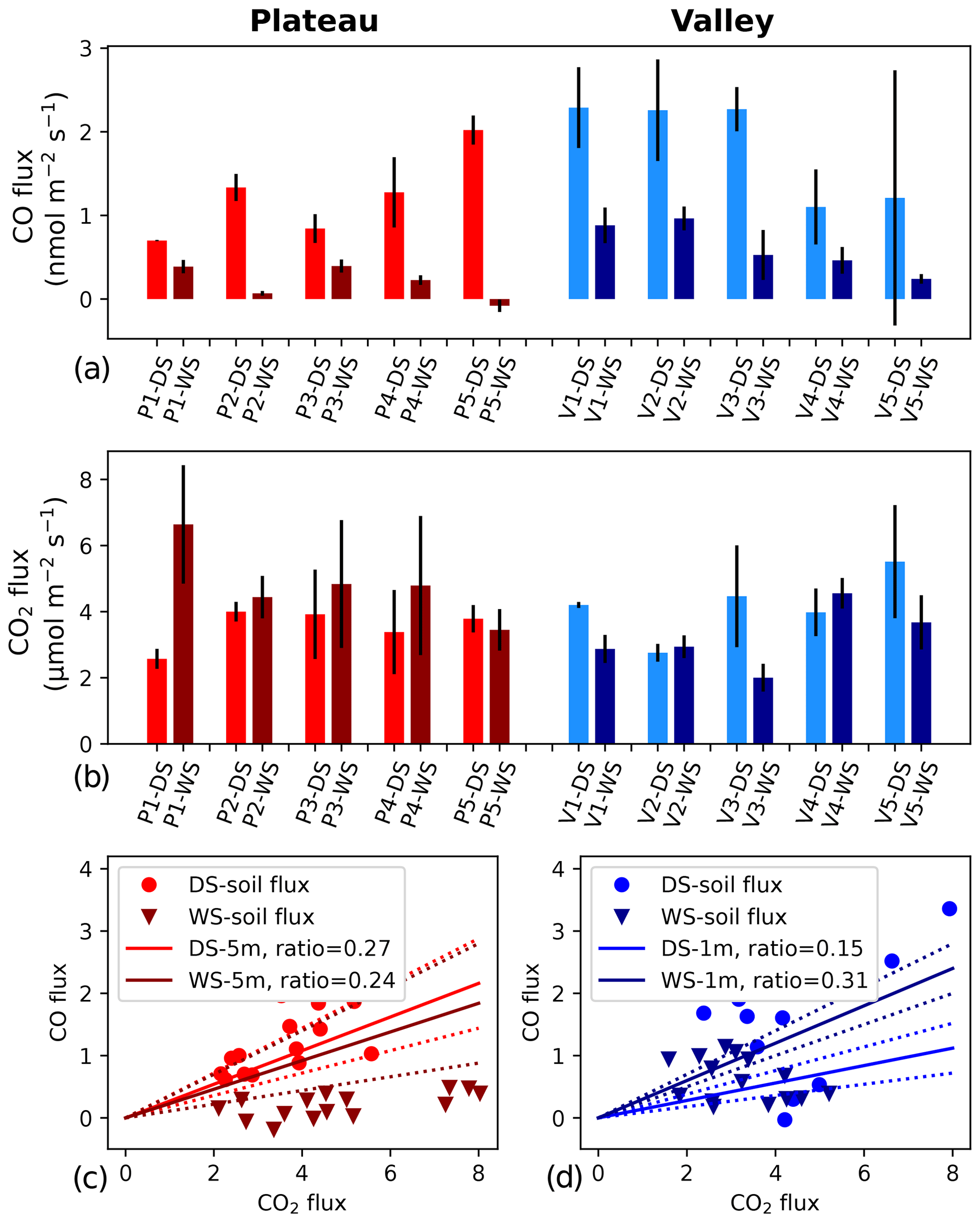
Figure 1 (a, b) CO and CO₂ soil fluxes at five different locations on the plateau (left, reddish colors) and in the valley (right, blueish colors). Lighter colors indicate dry season (DS), and darker colors indicate wet season (WS). Each location was measured 3 times during each campaign, and the error bars indicate the standard deviation of the mean of the three measurements. CO fluxes are based on bag mixing ratio measurements, and CO₂ fluxes are based on ICOS analyzer measurements. Panels (c) and (d) show the ratio between the soil CO and CO₂ fluxes (circles and triangles). In addition, the average DS and WS ratios as measured by the canopy layer budget method (tower height of 5 m) are shown as solid lines, and the standard deviations of these averages are indicated with dotted lines.

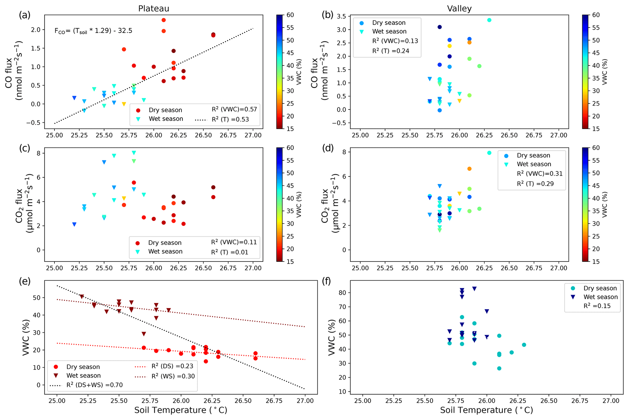
Figure 2 CO fluxes (nmol m⁻² s⁻¹) (a, b) and CO₂ fluxes (µmol m⁻² s⁻¹) (c, d) on the plateau (a, c) and in the valley (b, d). Dry-season measurements are indicated with circles, and wet-season measurements are indicated with triangles. Squared correlation coefficients between T (or VWC) and soil CO fluxes (or CO₂ fluxes) are given in the legend, and linear regression lines are shown for the cases where R²>0.50. The equation given in panel (a) indicates the relation found between the manual soil temperature measurements and the measured CO fluxes. (e, f) Relation between soil T and soil VWC, with the squared correlation coefficient given in the legend. In addition, three linear regression lines are shown for plateau measurements: for both campaigns together (DS + WS, R²=0.66) and for the individual campaigns DS (R²=0.23) and WS (R²=0.30). The shift in regression line indicates that plateau environmental drivers might differ between seasons.

Table 1 Overview of the soil chamber CO and CO₂ fluxes and the different ecosystem CO flux estimates. (a) The first three rows show the soil CO and CO₂ fluxes (range and mean (sd)) and their $\mathrm{\Delta }\mathrm{CO}/\mathrm{\Delta }{\mathrm{CO}}_{\mathrm{2}}$ as measured with the flux chamber technique. Each location had five collars and was measured 3 times per campaign (n=15). (b) The fourth row shows the $\mathrm{\Delta }\mathrm{CO}/\mathrm{\Delta }{\mathrm{CO}}_{\mathrm{2}}$ ratios of the nighttime increase on which the estimated ecosystem CO fluxes (fifth row) are based (range and mean (sd)). On the plateau, for each campaign night (DS: nine nights; WS: 7 nights), the ratios of five 2 h time windows were calculated; the average is based on time windows with ratios with R²>0.90. In the valley, for each campaign night, the ratio of one 9 h time window was used; the average is based on the nights with ratios with R²>0.90 (n=4 in DS, n=5 in WS). (c) The sixth row shows the vertical profile dCO-36m values on which the estimated ecosystem CO fluxes are based (seventh row). The range and mean (sd) are given of the four DS nights and the five WS nights (same as shown in Fig. 4) with six time windows per night (n=24, n=30). DS stands for dry season, and WS stands for wet season. Vertical profiles were not determined (n.d.) in the valley.

3.2 Atmospheric CO mixing ratios and ecosystem CO flux estimates

Dry-season CO campaign mixing ratios varied between 127 and 292 ppb (Fig. 3). Mixing ratios between the different heights generally followed a common pattern, indicating that air masses with elevated CO passing the tower are also reaching lower forest levels. Wet-season campaign CO mixing ratios ranged between 94 and 250 ppb and generally showed less variation, fewer peaks and lower mixing ratios. It is expected that (part of) the elevated mixing ratios and passing peaks in the dry season can be explained by the presence of biomass burning plumes, which can be transported over long distances (Andreae et al., 2012). The CO mixing ratio patterns, and the possible trajectories and dispersion of these biomass burning plumes, are the subject of ongoing research and will not be further discussed in this study.

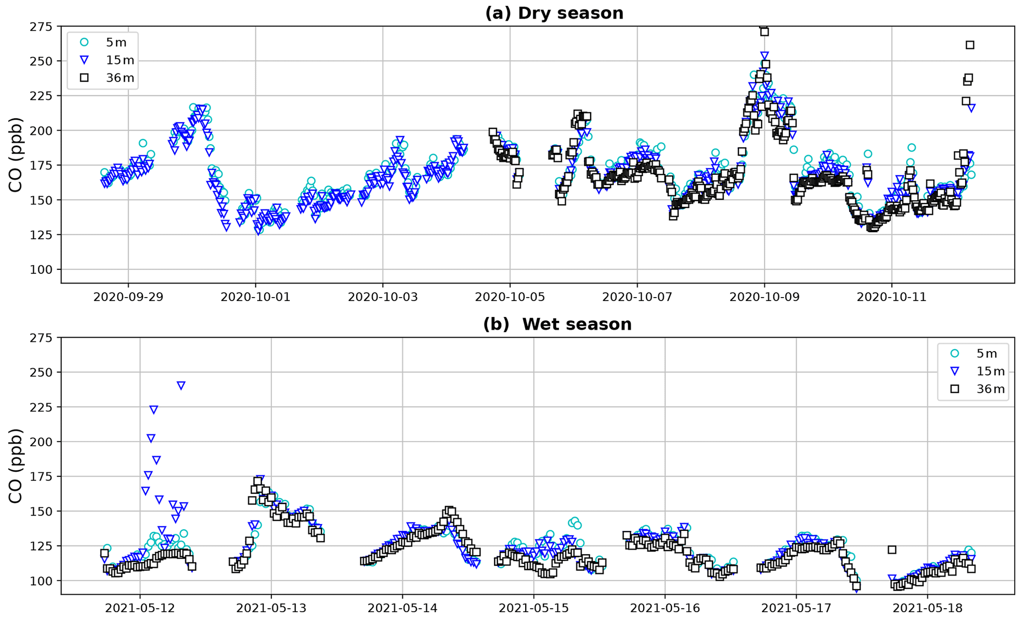
Figure 3 Tower CO mixing ratios during the dry-season campaign (a) and the wet-season campaign (b). Canopy height is ∼ 35 m. During the first 5 d of the dry season campaign, a leak was present in the 36 m inlet line, which is why data from this height are missing. Despite the variation, a general tendency with higher CO mixing ratios below the canopy is visible during both periods.

Vertical profiles per 1 h time window are shown in Fig. 4, vertical profiles per 1 h time window are shown in Fig. B2. In the dry season, four out of seven nights showed constant decreases in CO mixing ratio from 5 to 36 m, i.e., consistently negative dCO-36m during the whole night. Average nighttime dCO-36m values for these nights were −10.5, −8.1, −10.9 and −7.0 ppb (6, 7, 9 and 10 October; Fig. 4). In the wet season, vertical nighttime profiles generally showed smaller variation in CO mixing ratios; however, five out of seven nights still showed consistently decreasing CO mixing ratios with height over the whole night. In addition, only three 1 h time windows showed a dCO-36m value <0.9 ppb (2σ), which is regarded as the detection limit of the method. Average dCO-36m values for these nights were generally smaller than in the dry season: −2.5, −5.6, −4.6 and −2.3 ppb (13, 15, 16 and 17 May, respectively), with the exception of 14 May (−12.9 ppb) (Table 1, Fig. 4). Since no micro-meteorological measurements are available for the campaign periods, we cannot hypothesize why the night of 14 May was divergent.

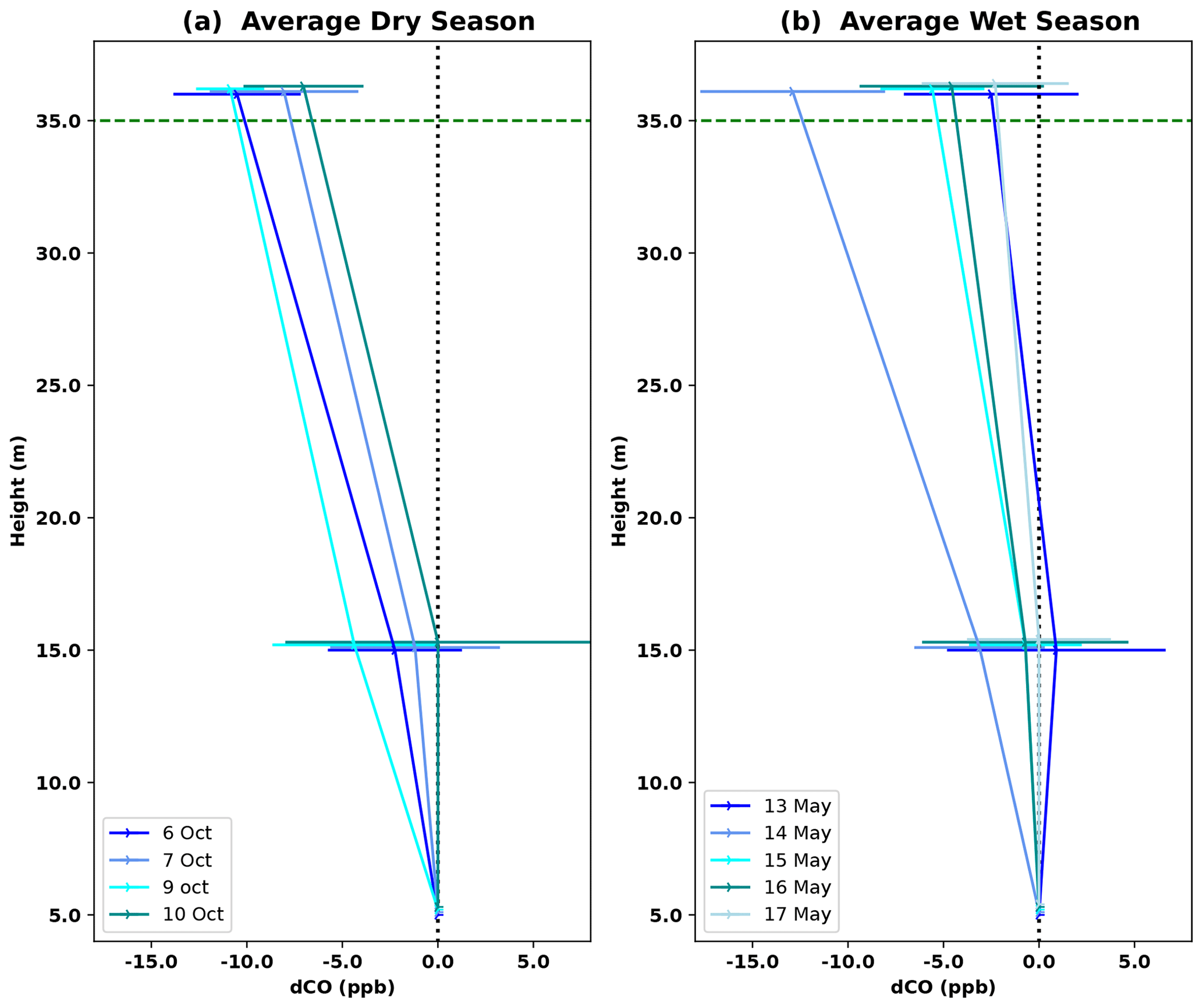
Figure 4 Average vertical CO profile for DS campaign nights (a) and WS campaign nights (b). Error bars indicate the standard deviation of dCO-15m and dCO-36m for the six 1 h time windows per night; this average was only calculated if dCO-36m was consistently negative over the whole night. Individual 1 h profiles per night are shown in Fig. B2. The dotted black vertical line indicates the zero line (dCO=0), and the dotted green horizontal line indicates the height of the canopy.

The canopy layer budget method was applied to the plateau inlet heights of 5 and 15 m and to the valley inlet height of 1 m. All ΔCO₂ and ΔCO values of the 2 h time windows (plateau) and the 3 h time windows (valley) were higher than the set detection limit of 2σ (ΔCO₂ > 0.1 ppm, ΔCO > 0.9 ppb). For the plateau, calculated $\mathrm{\Delta }\mathrm{CO}/\mathrm{\Delta }{\mathrm{CO}}_{\mathrm{2}}$ ratios with an R²>0.9 were selected, which was 29 % and 45 % of the cases in the dry season and 41 % and 40 % of the cases in the wet season for 5 and 15 m, respectively. Dry-season $\mathrm{\Delta }\mathrm{CO}/\mathrm{\Delta }{\mathrm{CO}}_{\mathrm{2}}$ ratios were slightly higher than wet-season ratios, but differences were not significant (Table 1). Applying Eq. (4) to the 5 m mean nighttime ratios (DS = 0.27 and WS = 0.24) gives a plateau ecosystem net production estimate of 2.1 and 1.9 nmol CO m⁻² s⁻¹ for the dry and wet season, respectively. For the valley measurements, squared correlation coefficients (R²) between ΔCO and ΔCO₂ were >0.75 on eight out of nine nights (four nights with R²>0.9), and, in the wet season, six out of seven nights reached R²>0.75 (five nights with R²>0.9). The wet-season ratios were significantly higher than the dry-season ratios, and applying Eq. (4) to the mean ratios leads to estimates of a net valley CO production of 1.1 and 2.3 nmol m⁻² s⁻¹ for the dry and the wet season, respectively (Table 1).

3.3 Laboratory results

Senescent leaves exposed to different temperatures emitted significant amounts of CO at rates increasing exponentially with higher temperatures. At 25 °C, average emission rates of 0.006 and 0.002 nmol CO g${}_{\mathrm{leaves}}^{-\mathrm{1}}$ min⁻¹ were measured for plateau and valley samples, respectively. The estimated ecosystem CO production rates, based on these average emission rates and senescent-leaf density in the literature (Luizão et al., 2004), are 0.012 and 0.002 nmol CO m⁻² s⁻¹ at 25 °C for the plateau and valley ecosystem, respectively (Fig. 5). The plateau soil material showed clear CO production increasing with higher temperatures. The valley soil material also showed CO production, but, due to instrument problems, a complete and consistent data set could not be collected. For plateau soil material, emissions of 0.0005 nmol CO g${}_{\mathrm{soil}}^{-\mathrm{1}}$ min⁻¹ at 25 °C were measured. The estimated ecosystem emissions coming from a plateau soil layer of 10 cm (Marques et al., 2013) at 25 °C were estimated to be ∼ 0.9 nmol CO m⁻² s⁻¹ (Fig. 5).

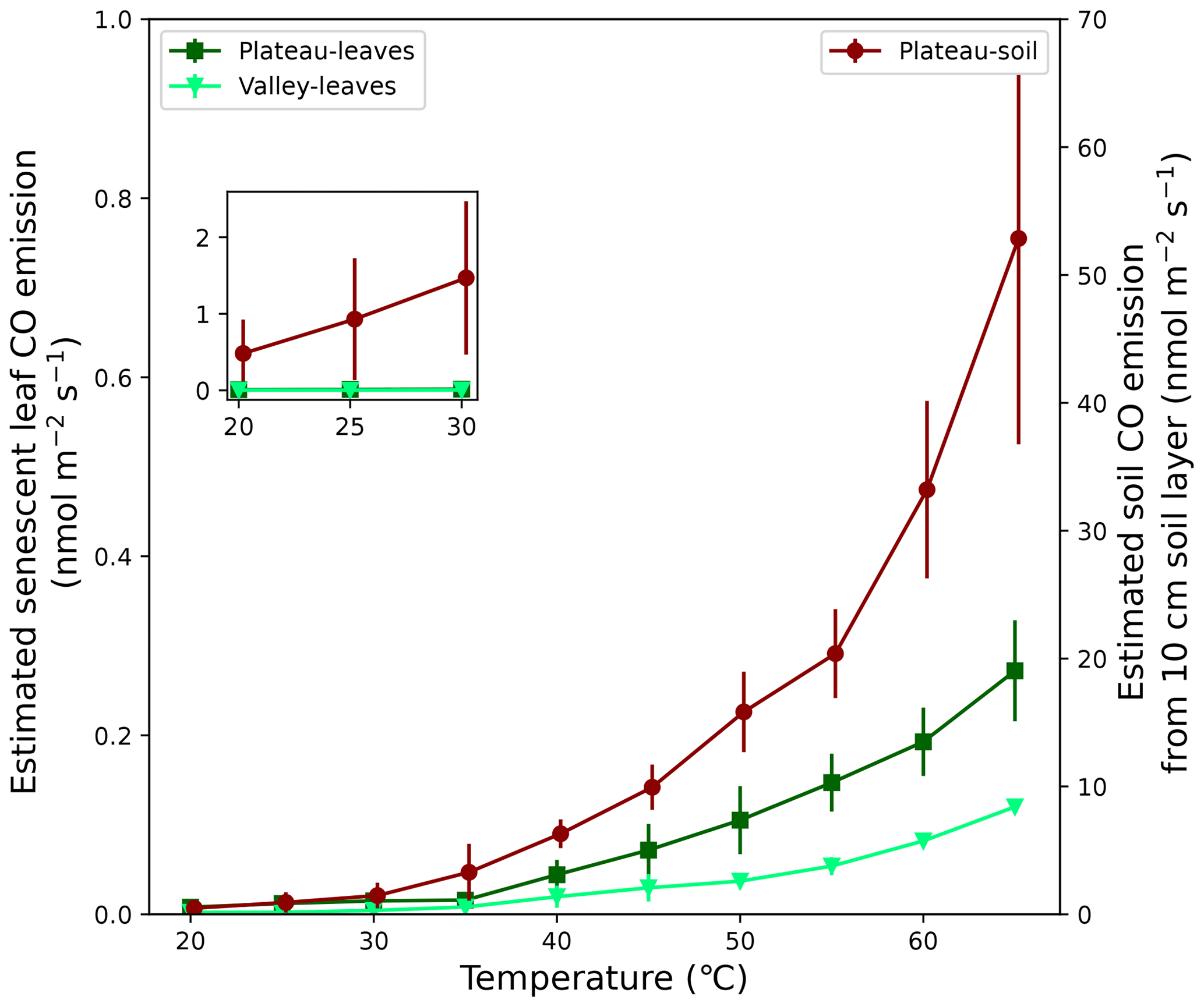
Figure 5 Expected CO emission of soil and senescent-leaf material expressed per surface area. For senescent-leaf CO emission (left axis; green triangles and squares), the laboratory CO emissions (nmol g${}_{\mathrm{leaves}}^{-\mathrm{1}}$ min⁻¹) were converted to seconds (s⁻¹) and were multiplied by a senescent-leaf density of 117 and 67 g_leaves m⁻² for the plateau and valley ecosystem, respectively (Luizão et al., 2004), so that CO production is expressed in nmol m⁻² s⁻¹. For the estimate of CO emission of a 10 cm soil layer (right axis; dark-red diamonds), the laboratory emissions (nmol g${}_{\mathrm{soil}}^{-\mathrm{1}}$ min⁻¹) were converted to seconds (s⁻¹) and were combined with a soil bulk density of 1.05 g cm⁻³ (Marques et al., 2013) so that soil CO production is expressed in nmol m⁻² s⁻¹. The set-in figure shows a zoom-in of senescent-leaf and soil emissions, plotted on the same y-axis scale, visualizing the expected dominance of soil CO emissions over senescent-leaf CO emissions.

4 Discussion

Plateau and valley soil chambers, measuring the emission of soil and litter together, generally showed net emission of CO, except for one plateau collar in the wet season. On the plateau, grouped dry- and wet-season CO fluxes showed a relation with soil temperature (R²=0.53) and with soil VWC (R²=0.57). The relations for individual campaigns did not fit to this curve (Fig. 2): while this can be partly attributed to the limited variation in soil temperature and soil moisture values, which diminishes the clarity of correlations, it also suggests that the drivers influencing plateau CO production may differ between seasons. Moreover, the strong relation between soil T and soil VWC (R²=0.70) on the plateau did not permit the determination of which factor drives the soil CO flux variation. In the valley, the variation in soil T and soil VWC was even more limited, resulting in less-pronounced dependencies and overall low squared correlations (all R²<0.32; Fig. 2).

Abiotic CO production and microbial CO uptake should correlate positively with increasing soil temperatures (van Asperen et al., 2015b; Cowan et al., 2018; Derendorp et al., 2011; King, 2000; Lee et al., 2012; Moxley and Smith, 1998). While for microbial CO uptake the relationship is expected to have an optimum temperature (King, 2000), the abiotic thermal degradation fluxes are exponential (van Asperen et al., 2015b; Conrad and Seiler, 1985; Derendorp et al., 2011; Lee et al., 2012) so that CO production is expected to become dominant at higher temperatures (van Asperen et al., 2015b; Cowan et al., 2018; King, 2000; Moxley and Smith, 1998). The role of VWC is more complicated. On the one hand, lower soil VWC leads to higher soil diffusivity, enhancing the CO uptake, thereby shifting the balance to soil CO uptake. For example, at the same fieldsite, high local CO uptake was observed from termite mounds, which consist of dry porous material (van Asperen et al., 2021; Martius et al., 1993). On the other hand, the availability of soil moisture has a direct effect on microbial CO uptake. Several studies found a parabolic response, with soil CO uptake having an optimum at VWC ∼ 20 %–30 % (King, 2000; King and Hungria, 2002; Moxley and Smith, 1998). Based on the supposed decrease in CO uptake when VWC > 30 %, one would expect a shift towards more positive CO fluxes from the dry season to the wet season, which is the opposite of what is observed in our measurements (Fig. 1). Following this line of reasoning, we expect that the observed negative relation between VWC and soil CO fluxes is an indirect one, driven by the relation of soil T and soil VWC.

The laboratory experiment, isolating the effect of temperature on CO production of senescent leaves and soil material, indicated a clear exponential increase in CO emissions with temperature, as also reported by earlier studies (van Asperen et al., 2015b; Derendorp et al., 2011; Lee et al., 2012). By combining literature values with our laboratory results, a simple approximate calculation was done to estimate the CO emission of senescent leaves and soil material at 25 °C at the ecosystem scale. Senescent leaves in the amount expected in the surface litter layer (Luizão et al., 2004) were estimated to emit 0.012 and 0.002 nmol CO m⁻² s⁻¹ on the plateau and in the valley, respectively, and a 10 cm plateau soil layer (Marques et al., 2013) was estimated to emit 0.93 nmol CO m⁻² s⁻¹. This simple upscaling ignores the colocated simultaneous soil CO uptake and, more importantly, this estimate ignores the CO production of the entire soil column below. Soil CO uptake has been shown to be dominant in ecosystems under specific conditions, such as lower temperatures and porous conditions (King, 2000; Kisselle et al., 2002); therefore in-depth research for this specific ecosystem would be needed to improve this upscaling. Nevertheless, this simple “back-of-the-envelope” calculation already shows the potential of mineral soil to be a strong emitter of CO and suggests that the observed chamber fluxes, which were measured over soil and litter together, mainly reflect emissions from the soil.

The laboratory CO emissions, the chamber CO fluxes and the nighttime ecosystem CO increase all demonstrate net production of CO by this ecosystem. All observations were performed in the absence of solar radiation so that a photochemically induced CO production pathway, such as photodegradation of organic material or the oxidation of VOCs and hydrocarbons (Lee et al., 2012; Schade et al., 1999; Szopa et al., 2021; Tarr et al., 1995), is unlikely to have contributed to our fluxes. In addition, the thick canopy of these forests prevents much sunlight from penetrating into the lower canopy or reaching the forest floor. Besides thermal degradation, ozonolysis of unsaturated hydrocarbons can produce CO in the absence of radiation (Röckmann et al., 1998). However, CO produced via ozonolysis would be associated with a strong enrichment in δ¹⁸O, which was not observed in additional experiments (see Appendix A). Therefore, we can exclude that ozonolysis plays a major role in our ecosystem. Following this line of reasoning, supported by the clear observed relation between temperature and CO fluxes (Figs. 2 and 5), we conclude that thermal degradation is likely the main driver of the observed nighttime CO increase and measured flux chamber CO fluxes in this central Amazonian tropical rainforest. The possible presence of additional photodegradation-induced CO production during the daytime would lead to even higher net total CO fluxes, a process not yet studied for tropical rainforests.

Plateau and valley CO mixing ratios were used to estimate ecosystem CO fluxes, which was done by studying the vertical CO gradient (only on the plateau) and by applying a canopy budget method (plateau and valley). Both approaches were only applied to nighttime measurements, when atmospheric conditions are generally more stable and with locally produced gases “trapped” below the canopy so that mixing ratio changes are more pronounced (Araújo et al., 2002). Generally, the nighttime vertical CO gradients were negative, i.e., had higher mixing ratios closer to the forest floor in comparison to above-canopy mixing ratios (Fig. 4). The vertical gradient can be used to estimate an ecosystem flux by assuming a fixed canopy flushing rate of 90 % over a vertical column of 30 m, as measured at a similar fieldsite close by (Simon et al., 2005). Querino et al. (2011) applied the same method and assumptions to vertical CH₄ gradients, measured at the same tower, where they were shown to give comparable flux estimates to on-site eddy covariance CH₄ measurements. The vertical CO gradients suggest an ecosystem flux up to ∼ 2 nmol CO m⁻² s⁻¹, with vertical profiles generally indicating larger emissions in the dry season (Table 1, last rows). On the plateau, the canopy budget method showed no significant differences in $\mathrm{\Delta }\mathrm{CO}/\mathrm{\Delta }{\mathrm{CO}}_{\mathrm{2}}$ ratios between the dry and the wet season, and, based on the 5 m inlet, plateau CO fluxes were estimated to range between 1.25 and 4.13 nmol CO m⁻² s⁻¹ in the dry season and between 0.94 and 3.28 nmol CO m⁻² s⁻¹ in the wet season. The valley nighttime $\mathrm{\Delta }\mathrm{CO}/\mathrm{\Delta }{\mathrm{CO}}_{\mathrm{2}}$ ratios were generally lower in the dry season, and valley CO fluxes were estimated to range between 0.3 and 1.9 nmol CO m⁻² s⁻¹ and between 1.8 and 3.1 nmol CO m⁻² s⁻¹ for the dry and the wet season, respectively.

The vertical gradient approach and the canopy budget method, and their subsequent ecosystem estimates, are possibly affected by the varying background CO mixing ratios (Fig. 3). We attempted to adjust for these background variations by applying strict filters. As described above, for the ecosystem flux estimate based on $\mathrm{dCO}/\mathrm{d}z$, only nights when the dCO-36m was consistently negative over the entire night were selected for upscaling. For the canopy budget method, which is based on the temporal change (ΔCO) below the canopy, only consistent ΔCO changes with a strong squared correlation to ΔCO₂ were selected (R²>0.9), so CO variations caused by a change in background mixing ratios are removed. The fact that the filtered ratios are relatively constant between heights and nights gives us confidence that this approach indeed selects the CO mixing ratio trends which are caused by the local ecosystem. In addition, the valley CO and CO₂ mixing ratios are possibly affected by nighttime drainage from the plateau (Araújo et al., 2008; Tóta et al., 2008): Araújo et al. (2008) showed valley nighttime CO₂ pooling at the same fieldsite, with plateau CO₂ laterally transported below the canopy. If this pooling is happening for CO₂, it is not unlikely that other trace gases, such as CO, are also transported. We therefore expect that the valley $\mathrm{\Delta }\mathrm{CO}/\mathrm{\Delta }{\mathrm{CO}}_{\mathrm{2}}$ ratios are not affected or, in case only CO₂ is pooling, are underestimated, which would mean that valley CO emissions would be even higher. Thus, possible pooling would not affect our prediction that valleys are a net CO emitter.

The used PCO₂ of 7.8 µmol m⁻² s⁻¹, as reported by Chambers et al. (2004), is a general ecosystem value and not specified for season or topographic location. Different studies at this fieldsite have demonstrated differences in CO₂ fluxes between the plateau and the valley. For example, Araújo (2009) performed eddy covariance measurements on the plateau and in the valley and found that the valley PCO₂ was two-thirds of the plateau PCO₂ (7.2 vs. 4.8 µmol m⁻² s⁻¹). Comparing plateau and valley, Chambers et al. (2004) found that soil respiration at this fieldsite was even twice as high on the plateau but pointed out that the valley soil respiration fluxes are likely underestimated to an unknown degree. Zanchi et al. (2014) found an opposite pattern, with valley soil respiration being ∼ 1.5 times higher than plateau soil respiration, which is similar to that observed in our study in the dry season (Fig. 1). Since the degree and direction of soil and ecosystem CO₂ flux variation between seasons and topographies is unclear, a differentiation in PCO₂ could introduce additional uncertainties. For this reason, for this study, it was decided to use a fixed PCO₂ for all topographies and seasons.

An overview of the direct soil CO flux measurements and indirect ecosystem CO flux estimates is given in Table 1. A direct comparison of these values should be done with care. First of all, the soil flux measurements are performed during (warmer) daytime hours, while the ecosystem estimates are determined for cooler nighttime conditions, although temperature variations below the canopy in this ecosystem are generally small (<7 °C; Araújo et al., 2002). Secondly, the flux chamber measures soil and litter only, while the ecosystem estimates include all possible sources and sinks below the canopy. Most importantly, soil flux values are measured directly, while the ecosystem fluxes are indirect estimates. Nonetheless, for the dry season, the plateau soil CO fluxes and the ecosystem CO flux estimates agree on the sign and on the magnitude of the CO fluxes. Moreover, the $\mathrm{\Delta }\mathrm{CO}/\mathrm{\Delta }{\mathrm{CO}}_{\mathrm{2}}$ ratio of the plateau nighttime increase shows similar ratios to the soil fluxes (Fig. 1, Table 1). We therefore expect that, in the dry season, the plateau nighttime CO increase is mostly driven by soil emission. For the wet season, the plateau soil CO fluxes were a lot smaller than the estimated ecosystem CO fluxes, and the flux chamber even showed uptake at one location. Because of the decrease in soil CO fluxes, the soil flux $\mathrm{\Delta }\mathrm{CO}/\mathrm{\Delta }{\mathrm{CO}}_{\mathrm{2}}$ ratios strongly dropped, which was only weakly observed in the ecosystem $\mathrm{\Delta }\mathrm{CO}/\mathrm{\Delta }{\mathrm{CO}}_{\mathrm{2}}$ ratios (Fig. 1). The difference in flux magnitudes and ratios indicates that, in the wet season, the type of soil surface, as measured in our soil chamber, is probably not the main driver of the plateau nighttime CO increase. Possibly, the plateau soil CO fluxes have a large spatial variability, with our soil collars representing cooler, wetter spots than the surrounding area. In addition, the seasonal shift in correlations between soil T, soil VWC and plateau soil CO fluxes (Fig. 2, left column) suggests that different dominant drivers may come into play during the wet season. A more elaborate flux chamber campaign, with possible nighttime measurements, would be crucial to verify the different hypotheses above.

All three methods on the plateau indicate higher CO emissions in the dry season, although the difference is only significant for the direct soil flux measurements. Based on the relation between soil temperature and soil CO fluxes described earlier (Fig. 2), and the clear increase in CO production with temperature (Fig. 5), we expect that the generally higher soil temperatures in the dry season cause the difference in CO fluxes between seasons. While no meteorological data from the K34 tower are available for both campaign periods, measurements from the local airport (∼ 50 km distance) show that the dry-season campaign period had clearly higher temperatures and lower relative humidities in comparison to the wet-season campaign period (INMET, 2024). In addition, in Appendix B, typical plateau dry- and wet-season soil temperatures from this fieldsite are shown, which indicate that the general diurnal temperature pattern barely drops below the estimated soil CO uptake threshold temperature of 25.2 °C (Fig. 2), even at night or in the wet season (Fig. B1).

Just as on the plateau, the valley soil fluxes were significantly higher in the dry season. In the dry season, valley soil chamber CO fluxes and ecosystem CO flux estimates agree quite well (Table 1), indicating that the nighttime valley CO increase is driven by sources such as our measured valley soil surface. Nevertheless, in the wet season, a clear discrepancy between the soil chamber flux magnitude and the valley ecosystem estimate was observed, indicating that the nighttime CO increase is driven by additional sources that are not captured in the flux chambers. Since the wet season is characterized by frequent and high amounts of rainfall, the valley stream frequently floods its adjacent areas, and this was also observed for the area below the valley inlet. Streams and rivers are known to be sources of CO, either produced by photodegradation or by thermal degradation (Campen et al., 2023; Müller, 2015; Valentine and Zepp, 1993; Zhang et al., 2008; Zuo and Jones, 1997), so it is likely that our wet-season nighttime measurements were dominated by the nearby valley stream and its inundated areas. Based on our measurements alone, we do not speculate whether the stream CO fluxes are caused by nighttime thermal degradation CO fluxes or represent a delayed outgassing of photodegradation-produced CO. On the whole, based on our observations, we expect that the valley is a net source of CO, with generally higher soil emissions in the dry season but with likely higher overall ecosystem emissions in the wet season, due to the contribution of the valley stream and its inundated areas.

Our measured soil CO fluxes are generally higher compared to the limited previous soil CO flux studies performed in (sub-) tropical ecosystems. Kisselle et al. (2002) observed negative fluxes (uptake) of −0.31 to −0.07 nmol m⁻² s⁻¹ in the dry and wet seasons (Brazilian savanna, Cerrado biome, opaque chambers, not burned area). Sanhueza et al. (1994) found that Venezuelan grasslands were a net CO source of 0.6 nmol m⁻² s⁻¹, which turned into a small CO sink when plowed ($\sim -\mathrm{0.3}$ nmol m⁻² s⁻¹). Venezuelan forest soils were found to be a net sink ($\sim -\mathrm{4}$ nmol m⁻² s⁻¹) but a net source (∼ 0.1 nmol m⁻² s⁻¹) after deforestation and “conversion” into a scrub grass savanna (Scharffe et al., 1990). To our knowledge, only one previous study attempted to estimate tropical rainforest CO fluxes, namely Kirchhoff and Marinho (1990), in a fieldsite near ZF2 (Ducke Forest Reserve, ∼50 km). Kirchhoff and Marinho (1990) measured the vertical CO gradient below the canopy and observed higher concentrations close to the soil surface in comparison to canopy height (dCO of −10 ppb), which is similar to gradients observed in this study. Based on this gradient, they estimated a forest CO flux of ∼ 6 nmol m⁻² s⁻¹, implying that the forest is a source of CO.

By providing the first direct tropical rainforest soil CO flux measurements, and by complementing these observations with nighttime ecosystem mixing ratio measurements, we can confirm the hypothesis of Kirchhoff and Marinho (1990) and can state that tropical rainforest ecosystems are likely a net source of CO. By a simple upscaling (averaging seasons and topographical locations of soil CO fluxes; Table 1), we derive an average tropical rainforest soil emission of ∼ 1 nmol CO m⁻² s⁻¹. Our nighttime measurements indicate that the general ecosystem CO emissions are possibly higher than this value, since valley streams, inundated soils and swampy areas, which are abundant in these ecosystems, might represent local hot spots. Translating our soil (and ecosystem) CO flux estimate to a yearly value gives an estimate of 0.9 g CO m⁻² yr⁻¹, and, by assuming a tropical rainforest area of 17.8×10⁶ km² (“global tropical (evergreen) forest”; Liu et al., 2018, Table 4), total global tropical rainforest emissions of ∼ 16.0 Tg CO yr⁻¹ are estimated.

By an innovative combination of methods and instruments, we were able to study the CO mixing ratios and fluxes over different temporal and spatial scales, even in a remote, challenging ecosystem such as a tropical rainforest. In the absence of a mobile CO analyzer, a more logistically challenging bag sampling design had to be employed, which is why the number of CO flux and mixing ratio measurements remains small, especially in the valley. By only focusing on 2 campaign weeks and two locations in a tropical rainforest, we realize that our study presents only a snapshot of the complex CO dynamics of a tropical rainforest. Nevertheless, our unique set of measurements shows that tropical forests are a net source of CO, likely dominated by soil CO emissions. In addition, in valley areas, river and water sources are expected to contribute to the overall ecosystem CO emissions. To further improve our understanding of the CO dynamics of a tropical rainforest, more in situ tropical forest soil and ecosystem CO flux measurements are needed, focusing on the possible complex dependencies between CO fluxes, (soil) temperature and soil moisture, and other environmental variables. Moreover, the role of soil type (e.g., texture, organic matter layer, porosity) and the significance of streams and inundated areas should be investigated. With the recent availability of mobile CO analyzers, we anticipate more in-depth studies, focusing on the different temporal and spatial scales of tropical rainforest CO fluxes.

5 Conclusions

By providing the first direct CO flux measurements of tropical rainforest soils, we can show that, in this ecosystem, soil CO production generally dominates over soil CO uptake. Complementary measurements of nighttime CO mixing ratios also suggest overall net ecosystem CO emissions, and estimated ecosystem CO fluxes were of the same sign and of similar magnitude to the measured soil CO fluxes. Thus, we can state that tropical rainforest ecosystems are likely a net source of CO, and we expect that soil emissions are the main contributor to the ecosystem CO emissions.

We observed that higher net soil CO emissions were accompanied by higher soil temperatures, and the warmer dry season generally showed larger soil and ecosystem CO emissions. With an additional laboratory experiment, the effect of temperature on CO production of senescent leaves and soil material was studied. The results show the potential of the soil material to be a strong emitter of CO and indicate that the observed chamber fluxes, which were measured over soil and litter together, are mainly driven by the soil. By excluding a large contribution of the process ozonolysis or a radiation-induced CO production pathway, we expect that the observed CO fluxes are mainly produced by the process of thermal degradation.

By a simple upscaling, we provide a first observation-based tropical rainforest soil emission estimate of ∼ 1 nmol CO m⁻² s⁻¹ (0.9 g CO m⁻² yr⁻¹), which leads to estimated global tropical rainforest soil emissions of ∼ 16.0 Tg CO yr⁻¹. Total ecosystem CO emissions might still be higher, since valley streams and inundated areas might represent local hot spots. To further improve these tropical forest ecosystem CO emission estimates, and to understand the complex dynamics between soil uptake and emission and their dependencies on environmental variables, more in situ tropical forest soil and ecosystem CO flux measurements are essential.

Appendix A: CO production via ozonolysis

Ozonolysis is the process by which ozone (O₃) can initiate oxidation of unsaturated hydrocarbons via addition to the double bond. In subsequent reaction steps CO can be produced (Criegee, 1975; Paulson and Seinfeld, 1992). Ozonolysis can occur in the absence of radiation and is therefore a potential contributor to our observed ecosystem nighttime CO increase. Ozone is known to be isotopically strongly enriched in ¹⁸O and ¹⁷O, with a typical δ¹⁸O value of 80 ‰–100 ‰. Röckmann et al. (1998) demonstrated that CO produced via ozonolysis inherits the strong ¹⁸O and ¹⁷O enrichment of O₃ because one of the O atoms is transferred from O₃ to CO. By determining the δ¹⁸O of the CO increase at night, the contribution of ozonolysis can be assessed.

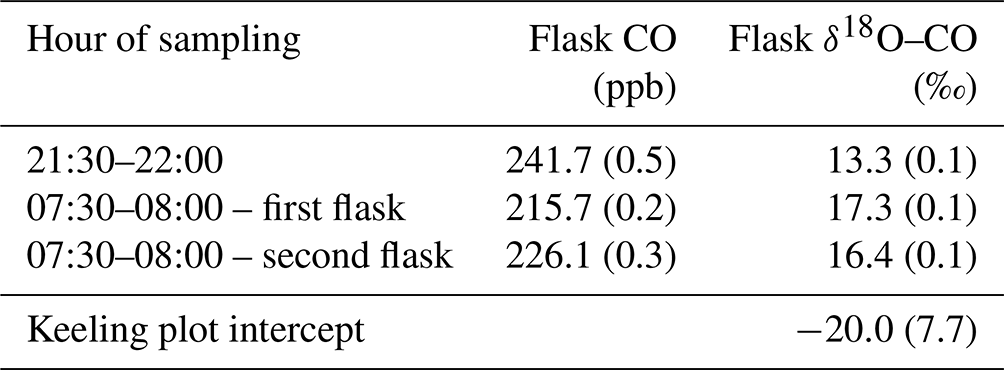
To investigate the potential contribution of ozonolysis to nighttime CO production, additional measurements were performed in September 2022 in the same valley where the nighttime valley CO increase was observed. A Teflon line (∼ 5 m) was placed at ∼ 2 m from the valley stream, at 1 m height. This line was sampled during four time windows: 17:00–17:30 (just before sunset), 21:00–21:30 and 21:30–22:00 (nighttime), and 07:30–08:00 (just after sunrise), with all times being in LT (UTC−4). Two pressurized air flasks (1 L) were sampled per time window, using a manual flask sampler (Heimann et al., 2022). To determine the isotopic composition of CO, these eight flasks were sent to the isotope laboratory at the Institute of Marine and Atmospheric Research Utrecht (IMAU) of Utrecht University. Unfortunately, several flasks broke during transport, and only three flasks (one night flask and two morning flasks) could be analyzed for CO and its isotopic composition (Table A1). A Keeling plot of these values results in an intercept of −20.0 ‰. Even though only three samples could be analyzed for isotopic composition, and the increase in CO is only 20–30 ppb, the Keeling plot analyses show that the higher nighttime CO concentrations are not accompanied by an enrichment in δ¹⁸O, which would be expected if the CO was produced by ozonolysis of unsaturated non-methane hydrocarbons (Röckmann et al., 1998). Having excluded ozonolysis as a significant contributor, we attribute the nighttime CO production to thermal degradation.

Table A1 Sampling time of flask, measured CO mixing ratios (with sd in brackets) and δ¹⁸O–CO of flasks (with sd in brackets).

Appendix B: Soil CO flux as a function of soil temperature

Continuous soil temperature measurements were not available for the campaign periods in 2020 and 2021. Fortunately, soil temperature measurements were available for most of the year 2019. Soil temperatures at different depths were monitored in 10 min intervals (STP01, Hukseflux). From previous measurements at the fieldsite, it was observed that the plateau soil temperature, measured with the manual sensor TP-101, agreed well with the continuous soil temperature measurements at 2 cm depth (differences generally <0.2 °C).

A simple soil-temperature-based diurnal CO flux pattern was estimated by use of the equation shown in Fig. 2 ($F_{\mathrm{CO}}=T_{\mathrm{soil}}\cdot \mathrm{1.29}-\mathrm{32.5}$), which indicates that soil CO uptake starts to dominate (the net flux turns from positive to negative) when temperatures drop below 25.2 °C. Figure B1 shows the average soil temperatures of May and November 2019 (left y axis) and the calculated soil CO flux (right y axis). These months were chosen because they were close to the campaign months of 2020 and 2021 (May and October) and because they presented an uninterrupted data set for the complete month.

While the average monthly temperatures did not drop below the threshold of 25.2 °C, individual nights sometimes showed lower temperatures. The standard deviation of the average temperature (not shown) was used to estimate a CO flux range (dotted lines), which shows that soil CO uptake can occur in the wet season and in the dry season. The daily averaged dry season (November) and wet season (May) flux was 1.22 and 0.63 nmol CO m⁻² s⁻¹, respectively, indicating that, based on this simple model, tropical forest soils are generally a CO source year round.

Figure B1 Left y axis: average soil temperature at 2 cm depth in the dry season (DS) of 2019 (October) and the wet season (WS) of 2019 (May) (standard deviations of the average soil temperatures are not shown). Right y axis: modeled soil CO flux for the DS and WS (solid lines) and its standard deviations (dotted lines) based on the soil temperatures (and their standard deviation) at 2 cm depth (equation shown in Fig. 2). The monthly mean calculated CO flux for the DS and WS is given in the legend and is in nmol CO m⁻² s⁻¹.

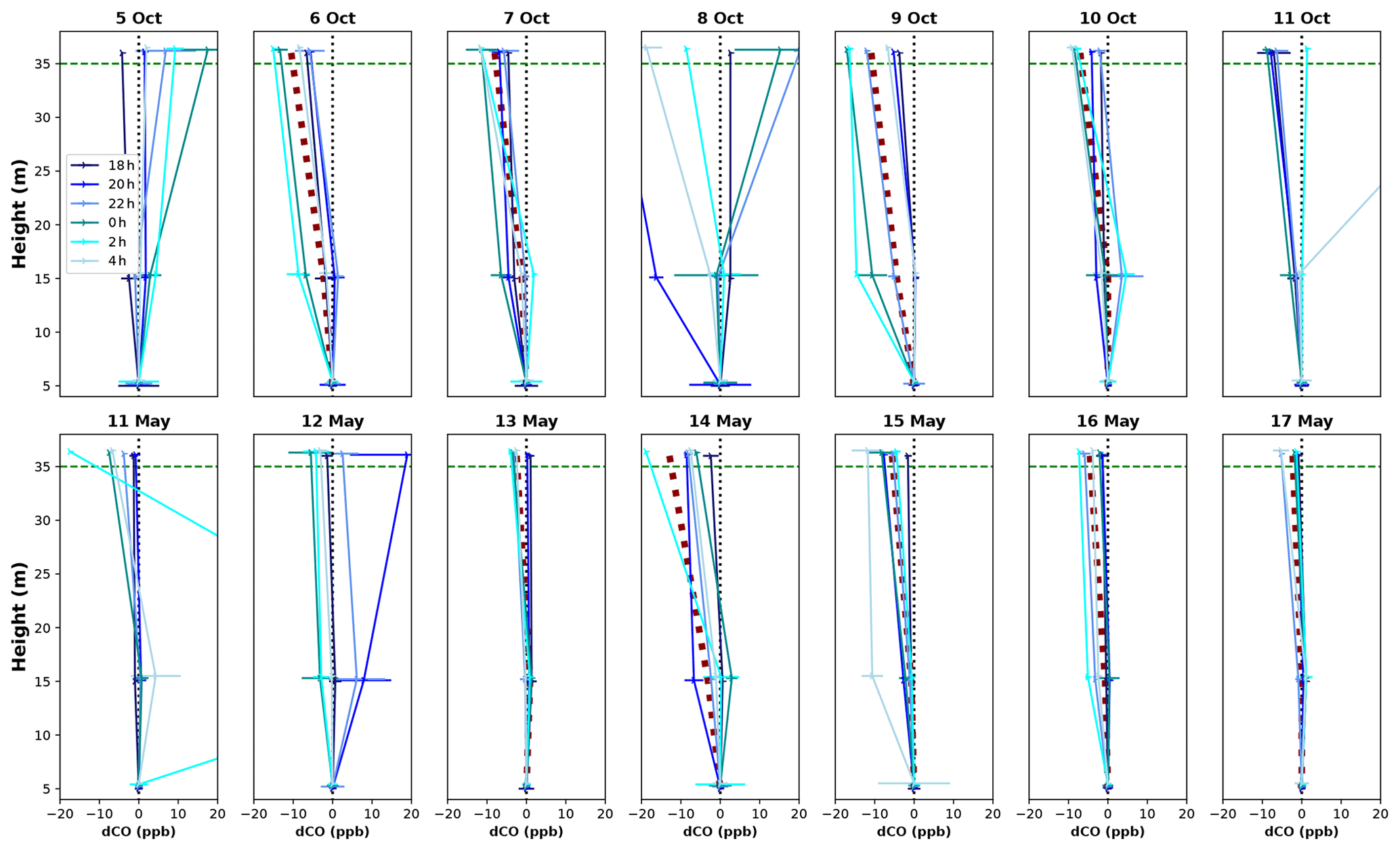
Figure B2 Vertical CO profiles for each DS campaign night (upper row) and WS campaign night (lower row). Each line shows the average vertical profile of that 1 h time window, and error bars indicate the standard deviation of the average of the three measurements in that time window. The dotted black vertical line indicates the zero line (dCO=0), and the dotted green horizontal line indicates the height of the canopy. The night of 11–12 May showed a strong CO peak at 15 m after midnight (also visible in Fig. 3), which we cannot explain.