Climatic controls on metabolic constraints in the ocean

Observations and models indicate that climate warming is associated with the loss of dissolved oxygen from the ocean. Dissolved oxygen is a fundamental requirement for heterotrophic marine organisms (except marine mammals) and, since the basal metabolism of ectotherms increases with temperature, warming increases organisms' oxygen demands. Therefore, warming and deoxygenation pose a compound threat to marine ecosystems. In this study, we leverage an ecophysiological framework and a compilation of empirical trait data quantifying the temperature sensitivity and oxygen requirements of metabolic rates for a range of marine species (“ecotypes”). Using the Community Earth System Model Large Ensemble, we investigate how natural climate variability and anthropogenic forcing impact the ability of marine environments to support aerobic metabolisms on interannual to multi-decadal timescales. Warming and deoxygenation projected over the next several decades will yield a reduction in the volume of viable ocean habitats. We find that fluctuations in temperature and oxygen associated with natural variability are distinct from those associated with anthropogenic forcing in the upper ocean. Further, the joint temperature–oxygen anthropogenic signal emerges sooner than temperature and oxygen independently from natural variability. Our results demonstrate that anthropogenic perturbations underway in the ocean will strongly exceed those associated with the natural system; in many regions, organisms will be pushed closer to or beyond their physiological limits, leaving the ecosystem more vulnerable to extreme temperature–oxygen events.

1 Introduction

Dissolved oxygen (O₂) is a fundamental metabolic requirement for heterotrophic marine organisms, excluding marine mammals (Pörtner, 2002; Keeling et al., 2010; Tiano et al., 2014). The decline in ocean O₂ due to warming is a tendency that has been long predicted by models (Keeling et al., 2010; Long et al., 2016; Oschlies et al., 2018) and that was recently found to be evident at the global scale in compilations of in situ observations (Schmidtko et al., 2017; Ito et al., 2017). Deoxygenation is driven by the direct effect of reduced oxygen solubility with warming, compounded by buoyancy-induced stratification in the upper ocean, which weakens the ventilation-mediated supply of fresh oxygen to the ocean interior. While the full ecological implications of ocean deoxygenation remain uncertain, it is clear that the physiological impacts of oxygen loss on marine organisms can be considered explicitly in the context of warming: basal metabolic rates for ectothermic organisms depend on ambient temperature and increase with warming (Gillooly et al., 2001); thus, higher temperatures impose additional demands for oxygen to sustain aerobic respiration (Deutsch et al., 2015). Consequently, as the ocean warms, even present-day oxygen distributions may be insufficient to meet the oxygen demands of organisms living near key physiological thresholds (Deutsch et al., 2022).

Model projections clearly demonstrate that warming and deoxygenation are consequences of human-driven climate change, yet natural climate variability also produces important fluctuations in these quantities. Indeed, evidence suggests that natural variability contributes to hypoxic events, such as those observed in the California Current, where fish and benthic-organism mortality has been associated with low-O₂ waters impinging on the continental shelf (Pozo Buil and Di Lorenzo, 2017; Howard et al., 2020). A clear understanding of how natural climate variability drives fluctuations in metabolic state and the associated implications for organisms is a critical context in which to view long-term climate warming. Given that the natural system is highly dynamic, climate change signals are often masked by decadal-scale variability (Ito and Deutsch, 2010). While numerous authors have considered the detection and attribution of climate change for physical and biogeochemical variables (Rodgers et al., 2015; Long et al., 2016; Schlunegger et al., 2019), comparatively little attention has been devoted to explicitly characterizing the relative influence of natural and anthropogenic drivers of changes in the ocean's capacity to support aerobic life. In this study, we approach this challenge by leveraging the concept of the metabolic index (Φ) introduced by Deutsch et al. (2015). Φ is based on the notion that aerobic organisms can persist only where the ambient oxygen partial pressure (pO₂) is sufficient to sustain respiration. Φ incorporates an explicit representation of the dependence of metabolic oxygen demand on temperature, thus providing a framework to consider how joint oxygen and temperature variability constrain viable habitats in the ocean.

Many ocean organisms may already be under threat from deoxygenation (Hoegh-Guldberg and Bruno, 2010; Breitburg et al., 2018); however, ongoing climate-driven loss of oxygen raises important questions about the future of marine ecosystems: how will anthropogenic changes in dissolved oxygen and temperature affect the capacity of ocean habitats to support aerobic metabolism? What are the spatial and temporal distributions of changes in the ocean's metabolic state associated with climate variability? At what point can anthropogenic change in the ocean's metabolic state be distinguished from natural variability? This study addresses these questions using a combination of metabolic theory; a dataset quantifying key physiological parameters for a collection of marine species adapted to specific environments (“ecotypes”); and the oxygen and temperature distributions as simulated in the Community Earth System Model, version 1, Large Ensemble (CESM1-LE), which includes 34 members simulating ocean biogeochemistry under climate variability and change for the period 1920–2100, forced using historical data and the Representative Concentration Pathway Scenario 8.5 (RCP85) (Kay et al., 2015; Long et al., 2016).

This paper is organized as follows. Section 2 presents a brief overview of the relevant metabolic theory and the associated empirical datasets and describes our approach to the analysis. In Sect. 3, we present results quantifying the joint temperature–oxygen variability simulated in the CESM1-LE, evaluating the spatiotemporal structure of variability in marine ecotype habitats, including long-term trends based on the RCP8.5 scenario and time of emergence (ToE). The main outcomes of the results are synthesized in Sect. 4 and summarized in Sect. 5.

2 Datasets and methods

2.1 Metabolic index

Empirical studies measuring thermal tolerance and oxygen requirements in the laboratory for an array of marine organisms have enabled an assessment of lethal thresholds (Vaquer-Sunyer and Duarte, 2008; Rosewarne et al., 2016). These data, coupled with recent advances in the theoretical frameworks, enable both explanatory and predictive power in the context of a dynamic environment (Deutsch et al., 2015; Penn et al., 2018; Howard et al., 2020). The fundamental insights here are that basal metabolic rates for ectothermic marine organisms depend on ambient temperature and generally increase with warming (Gillooly et al., 2001). Increasing basal metabolic rates impose additional demands for oxygen. Organisms use oxygen dissolved in seawater, and acquisition tends to be limited by diffusive processes; thus, oxygen supply is related to the ambient pO₂. The ratio of oxygen supply to temperature-dependent demand provides a critical indicator of the capacity for an organism to meet its metabolic requirements. Deutsch et al. (2015) formalized these concepts into a quantity termed the metabolic index (Φ), which is defined as the ratio of oxygen supply to an organism's resting metabolic demand. Oxygen supply is parameterized according to a biomass-dependent scaling of pO₂, capturing variations in the efficiency with which organisms acquire and utilize O₂. This can be expressed as $S={\widehat{\mathit{\alpha }}}_{\mathrm{s}}{B}^{\mathit{\sigma }}p{\mathrm{O}}_{\mathrm{2}}$, where ${\widehat{\mathit{\alpha }}}_{\mathrm{s}}$ represents the gas transfer between an organism and its environment, and B^δ is the scaling of supply with biomass B (Piiper et al., 1971). Gas supply is represented as an Arrhenius function:

$$\begin{array}{}\text{(1)}& {\widehat{\mathit{\alpha }}}_{\mathrm{s}}={\mathit{\alpha }}_{\mathrm{s}}\exp \left\{{\displaystyle \frac{-E_{\mathrm{s}}}{K_{\mathrm{B}}}}\left[{\displaystyle \frac{\mathrm{1}}{T}}-{\displaystyle \frac{\mathrm{1}}{T_{\text{ref}}}}\right]\right\}.\end{array}$$

The resting metabolic demand is also expressed using the Arrhenius equation as follows:

$$\begin{array}{}\text{(2)}& D={\mathit{\alpha }}_{\mathrm{D}}{B}^{\mathit{\delta }}\exp \left\{{\displaystyle \frac{-E_{\mathrm{d}}}{K_{\mathrm{B}}}}\left[{\displaystyle \frac{\mathrm{1}}{T}}-{\displaystyle \frac{\mathrm{1}}{T_{\text{ref}}}}\right]\right\},\end{array}$$

where α_D is a species-specific basal metabolic rate, E_d (eV) is the temperature dependence of oxygen supply, T is temperature, T_ref is the reference temperature (15 °C), and k_B is the Boltzmann constant (Gillooly et al., 2001). Gas transfer is kinematically slow at low temperatures, and, hence, organism viability can be limited by the energy required to acquire oxygen at low temperatures; thus, E_o varies with temperature. Here, we account for this by adding the temperature dependence ($\mathrm{d}{E}_{\mathrm{o}}/\mathrm{d}T$) to E_o in the equations above ($E_{\mathrm{o}}+\frac{\mathrm{d}{E}_{\mathrm{o}}}{\mathrm{d}T}(T-T_{\text{ref}})$), using the mean value of $\mathrm{d}{E}_{\mathrm{o}}/\mathrm{d}T=\mathrm{0.022}$ eV, consistently with Deutsch et al. (2020). The metabolic index can thus be written as the ratio of $S/D$:

$$\begin{array}{}\text{(3)}& {\displaystyle }\begin{array}{rl}{\displaystyle }\mathrm{\Phi }=& {\displaystyle \frac{{\mathit{\alpha }}_{\mathrm{s}}}{{\mathit{\alpha }}_{\mathrm{D}}}}{\displaystyle \frac{B^{\mathit{\sigma }}}{B^{\mathit{\delta }}}}p{\mathrm{O}}_{\mathrm{2}}\\ {\displaystyle }& {\displaystyle }\times \exp \left\{{\displaystyle \frac{-E_{\mathrm{s}}}{K_{\mathrm{B}}}}\left[{\displaystyle \frac{\mathrm{1}}{T}}-{\displaystyle \frac{\mathrm{1}}{T_{\text{ref}}}}\right]+{\displaystyle \frac{E_{\mathrm{d}}}{K_{\mathrm{B}}}}\left[{\displaystyle \frac{\mathrm{1}}{T}}-{\displaystyle \frac{\mathrm{1}}{T_{\text{ref}}}}\right]\right\},\\ {\displaystyle }=& {\displaystyle }{A}_{\mathrm{o}}{B}^{\mathit{\sigma }-\mathit{\delta }}p{\mathrm{O}}_{\mathrm{2}}\exp \left\{{\displaystyle \frac{E_{\mathrm{d}}-E_{\mathrm{s}}}{K_{\mathrm{B}}}}\left[{\displaystyle \frac{\mathrm{1}}{T}}-{\displaystyle \frac{\mathrm{1}}{T_{\text{ref}}}}\right]\right\},\\ {\displaystyle }=& {\displaystyle }{A}_{\mathrm{o}}p{\mathrm{O}}_{\mathrm{2}}\exp \left\{{\displaystyle \frac{E_{\mathrm{o}}}{K_{\mathrm{B}}}}\left[{\displaystyle \frac{\mathrm{1}}{T}}-{\displaystyle \frac{\mathrm{1}}{T_{\text{ref}}}}\right]\right\},\end{array}\end{array}$$

where $A_{\mathrm{o}}={\mathit{\alpha }}_{\mathrm{S}}/{\mathit{\alpha }}_{\mathrm{D}}$ (atm⁻¹) is the hypoxic tolerance, and $E_{\mathrm{o}}=E_{\mathrm{d}}-E_{\mathrm{s}}$ (E_s is the temperature dependence of oxygen supply) (Deutsch et al., 2015; Penn et al., 2018). The exponent, $\mathit{\epsilon }=\mathit{\sigma }-\mathit{\delta }$, is the allometric scaling of the supply-to-demand ratio with biomass, and it is typically near zero. Therefore, in the analysis that follows, we presume unit biomass and thus neglect the potential impacts of variations in biomass.

If Φ falls below a critical threshold value of 1, conditions are physiologically unsustainable: an organism cannot meet its basic resting metabolic oxygen requirements. Conversely, values of Φ above 1 enable organismal metabolic rates to increase by a factor of Φ above resting levels, permitting critical activities such as feeding, defense, growth and reproduction. Thus, for a given environment and species, Φ provides an estimate of the ratio of the maximum sustainable metabolic rate to the minimum rate necessary for basal metabolism. Deutsch et al. (2015) inferred the ratio of active to resting energetic demand by examining the biogeographic distribution of several species, finding that range boundaries coincide with values of Φ=1.5–7. This threshold, termed the critical rate (Φ_crit), represents the minimum metabolic index required for an organism to sustain an active metabolic state, which is a more meaningful ecological threshold than requirements for resting metabolism. Therefore, in this study, we define a quantity Φ^′, derived by dividing Φ by Φ_crit so that, when Φ falls below 1, the organism can no longer sustain its active metabolic demand and will need to make physiological trade-offs. Accounting for these active metabolic requirements, we use an adjusted definition of the hypoxic tolerance trait, $A_{\mathrm{c}}=A_{\mathrm{o}}/{\mathrm{\Phi }}_{\text{crit}}$, where A_c is termed the “ecological hypoxia tolerance”, consistently with Howard et al. (2020). Where ${\mathrm{\Phi }}^{\prime }>\mathrm{1}$ (i.e., Φ>Φ_crit), an organism can sustain an active metabolic rate; where ${\mathrm{\Phi }}^{\prime }<\mathrm{1}$ (i.e., Φ<Φ_crit), O₂ is insufficient, and an active metabolic state is not viable. Henceforth, our analysis focuses on Φ^′; in the subsequent text and figures, metabatic index refers to Φ^′ (${\mathrm{\Phi }}^{\prime }=\mathrm{\Phi }$) throughout.

2.2 Physiological dataset

We make use of a dataset describing physiological parameters for a collection of 61 marine ecotypes spanning a range of ecological hypoxic tolerances (A_c) and temperature sensitivities (E_o) (Penn et al., 2018; Deutsch et al., 2020, Fig. 1a). The 61 species span benthic and pelagic habitats across four phyla in all ocean basins (Arthropoda, Chordata, Mollusca and Cnidaria). The dataset includes 28 malacostracans, 21 fishes; three bivalves and cephalopods; two copepods; and one of each for gastropods, ascidians, scleractinian corals and sharks with body mass spans of 8 orders of magnitude (Penn et al., 2018). We illustrate how the physiological traits E_o and A_c constrain habitat viability in the context of distributions of pO₂ and temperature in the marine environment in Fig. 1b, which shows the minimum pO₂ (i.e., pO₂ at Φ_crit) required to sustain an active metabolic state as a function of temperature for five combinations of E_o and A_c. The five combinations are derived from sampling the probability distributions of E_o and A_c (Fig. 1a) at the 10th, 50th and 90th percentile values (illustrated by colored stars in Fig. 1a and corresponding curves in Fig. 1b). We assume that the trait distributions are independent, which is a reasonably modest simplification; E_o is represented by a normal distribution, and A_c is represented by a lognormal distribution function (Fig. S1 in the Supplement). The pO₂ at Φ_crit curves shown in Fig. 1b delineate regions of pO₂–temperature space that are habitable (above the curve) and uninhabitable (below the curve). The reversing curvature of pO₂ at Φ_crit in Fig. 1b at low temperatures captures the decrease in the organisms' oxygen acquisition efficiencies in cooler conditions, yielding cold intolerance. At very low temperatures, gas transfer is limited by the decrease in molecular gas diffusion; as a consequence, oxygen transfer into the organisms requires energy, yielding cold intolerance. This is well illustrated by the blue line in Fig. 1b.

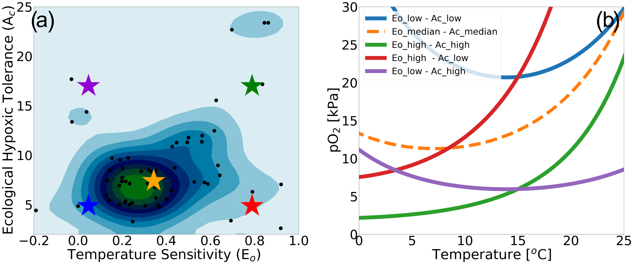
Figure 1 Physiological traits determining hypoxic tolerance. (a) Scatter plot of 61 marine ecotypes for which empirically derived estimates of activation energy (E_o) and the ecological hypoxic tolerance (A_c) have been determined (Penn et al., 2018). The color shows the density of occurrence for the 61 marine ecotypes in the A_c–E_o trait space. (b) The minimum pO₂ required to sustain an active metabolic state (i.e., pO₂ at Φ_crit; Deutsch et al., 2020) for five combinations of A_c and E_o, corresponding to the stars in panel (a); these are combinations of the 10th, 50th and 90th percentile values for each parameter. Below the pO₂ lines shown, the organism would experience an oxygen deficit relative to its active metabolism requirements, effectively signifying the species-specific hypoxic conditions, based on physiological traits, for this range of temperatures.

To illustrate how the trait combinations of E_o and A_c exert control on the geographic distribution of organisms in the marine environment (Deutsch et al., 2020), we use observations of pO₂ and T along a zonal transect of the Pacific Ocean and plot Φ^′ for nine combinations of E_o and A_c percentile values (Fig. 2). The color bars in Fig. 2a–i show the metabolic index for an active state (Φ^′); regions with values above 1 are habitable (colored), while regions with values below 1 are uninhabitable (white) on the basis of metabolic constraints (other ecological considerations are not considered). The subplots in the upper portion of the figure are arranged according to the same trait axes shown in Fig. 1a; E_o increases horizontally from left to right, and A_c increases from the bottom to the top. For the trait combination in the bottom left (low E_o, low A_c; Fig. 2g), metabolism is relatively insensitive to temperature, and tolerance for low pO₂ is poor. Thus, ecotypes with low E_o and low A_c are restricted to high-latitude surface waters, where temperatures are cool and where pO₂ is abundant (Fig. 2g). As E_o increases from left to right, metabolic rates become more sensitive to temperature. Then, habitat is gained at depth, where temperatures are cooler and where higher temperature sensitivity confers an advantage (Fig. 2g–i). From the bottom to the top, the increase in the tolerance of low-pO₂ conditions increases habitability in regions of low pO₂, enabling organisms to expand beyond high-latitude surface waters (Fig. 2g–a). The biogeographic range for organisms with high A_c is modulated by E_o; as temperature sensitivity increases, ecotype viability at high latitudes increases, but tropical surface waters become less viable (Fig. 2a–c). Henceforth, our analysis will utilize the metabolic index of the median ecotype (E_o=0.34, A_c=7.4; Fig. 2e) for illustrative purposes; i.e., all metabolic index figures refer to this median ecotype unless otherwise stated.

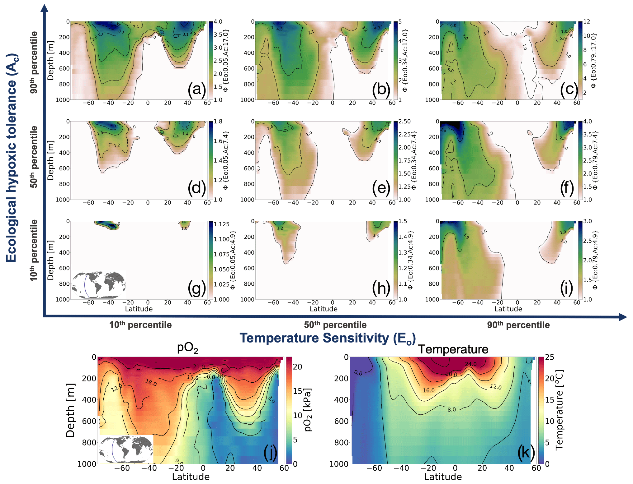
Figure 2 Annual mean metabolic index (Φ^′) for nine combinations of the ecological traits E_o (metabolic temperature sensitivity) and A_c (ecological hypoxic tolerance) along a transect in the Pacific Ocean based on a climatology from the World Ocean Atlas dataset (Garcia et al., 2014). The percentile values of each trait are as follows: 10th (E_o=0.04, A_c=4.8), 50th (E_o=0.34, A_c=7.4) and 90th (E_o=0.79, A_c=17.0). The lower panels show pO₂ and temperature from the WOA dataset. Note that the color bar range differs by panel and according to values where ${\mathrm{\Phi }}^{\prime }<\mathrm{1}$ is omitted; thus, the color shows only areas where an active metabolic state can be sustained.

2.3 Earth system model simulations

This study is based on the CESM1-LE, described in detail by Kay et al. (2015). The CESM1-LE included 34 ensemble members integrated from 1920–2100 under historical and RCP8.5 forcing. The ensemble was generated by adding round-off level (10⁻¹⁴ K) perturbations to the air temperature field at initialization in 1920; this small difference yields rapidly diverging model solutions due to the chaotic dynamics intrinsic to the climate system, thus developing an ensemble spread that is representative of internal variability (Kay et al., 2015). Briefly, the CESM1-LE uses the Community Earth System Model, version 1 (Hurrell et al., 2013), with a horizontal resolution of (nominally) 1° in all components. The ocean component is the Parallel Ocean Program, version 2 (Smith et al., 2010), with sea ice simulated by the Los Alamos Sea Ice Model, version 4 (Hunke and Lipscomb, 2010). Ocean biogeochemistry was represented by the Biogeochemical Elemental Cycling (BEC) model (Moore et al., 2013; Lindsay et al., 2014).

Our analysis focuses on three depths: 50 m, representing near-surface dynamics; the epipelagic zone at 200 m; and the mesopelagic zone at 500 m. pO₂ was calculated using the Garcia and Gordon (1992) solubility formulation. For convenience, we use the period 1920–1965 to define a minimally perturbed natural state as this period is prior to the development of substantial anthropogenic trends in ocean oxygen and temperature (Long et al., 2016). We also examine distributions over the last 3 decades of the 21st century (2070–2099) to evaluate the projected climate change signal under RCP8.5. We use the mean across all 34 ensemble members to quantify the deterministic, “forced” response of the climate system to anthropogenic influence (Deser et al., 2012). The ensemble spread is thus indicative of the amplitude of variations attributable to natural variability.

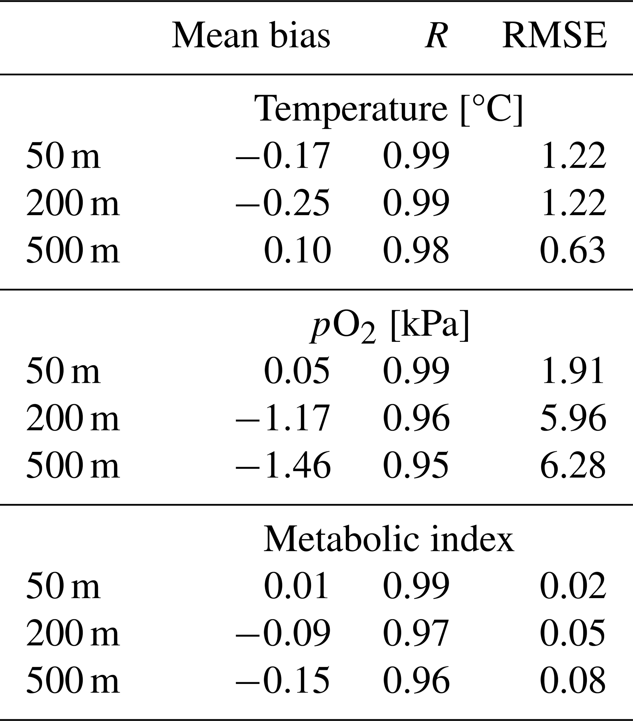
We compared the CESM1-LE (1920–1965) with the World Ocean Atlas, version 2013 (WOA2013), dataset (Garcia et al., 2014), an observationally based, gridded climatology (Fig. 3a–i). CESM1-LE generally provides a reasonable representation of pO₂ and temperature distributions at the selected depths (Fig. 3); however, there are important biases to acknowledge in the context of interpreting the results. Temperature magnitudes are generally well simulated in the CESM1-LE, showing a root mean square error (RMSE) of <1.3 °C and a pattern correlation coefficient of (PCC) >0.98 in all three selected depths (50, 200 and 500 m) (Table 1). Temperature magnitudes are slightly underestimated at 50 and 200 m (mean bias of <0.3 °C) and are overestimated by 0.41 °C at 500 m. Note that, since our comparison uses CESM1-LE data from the period 1920–1965, some discrepancy in temperature might be expected from the signal of climate warming present in the WOA observations. pO₂ is also reasonably well captured by the CESM1-LE (PCC<0.95), but magnitudes are slightly underestimated at depth, showing a mean bias of −1.63 and −2.1 kPa at 200 and 500 m with respect to WOA13 (Table 1). Regions of low-pO₂ waters are too extensive in CESM1-LE (Fig. 3n and o), and there is a slight degradation of skill with depth for pO₂ fields (Table 1). The underestimation of pO₂ leads to a slight underestimation of Φ^′ with respect to WOA13 and an overestimation of habitat loss in the future climate (Fig. 3p–r); however, Φ^′ computed from the model fields demonstrates that the dominant spatial patterns are well captured by the CESM1-LE despite magnitudes that are slightly too low. This CESM pO₂ bias is common among coarse-resolution ocean models, and it is attributed to a sluggish circulation and, hence, weak ventilation (Long et al., 2016). These differences ultimately matter most near the hypoxic zones and at the boundaries of habitable zones like the oxygen minimum zones (OMZs).

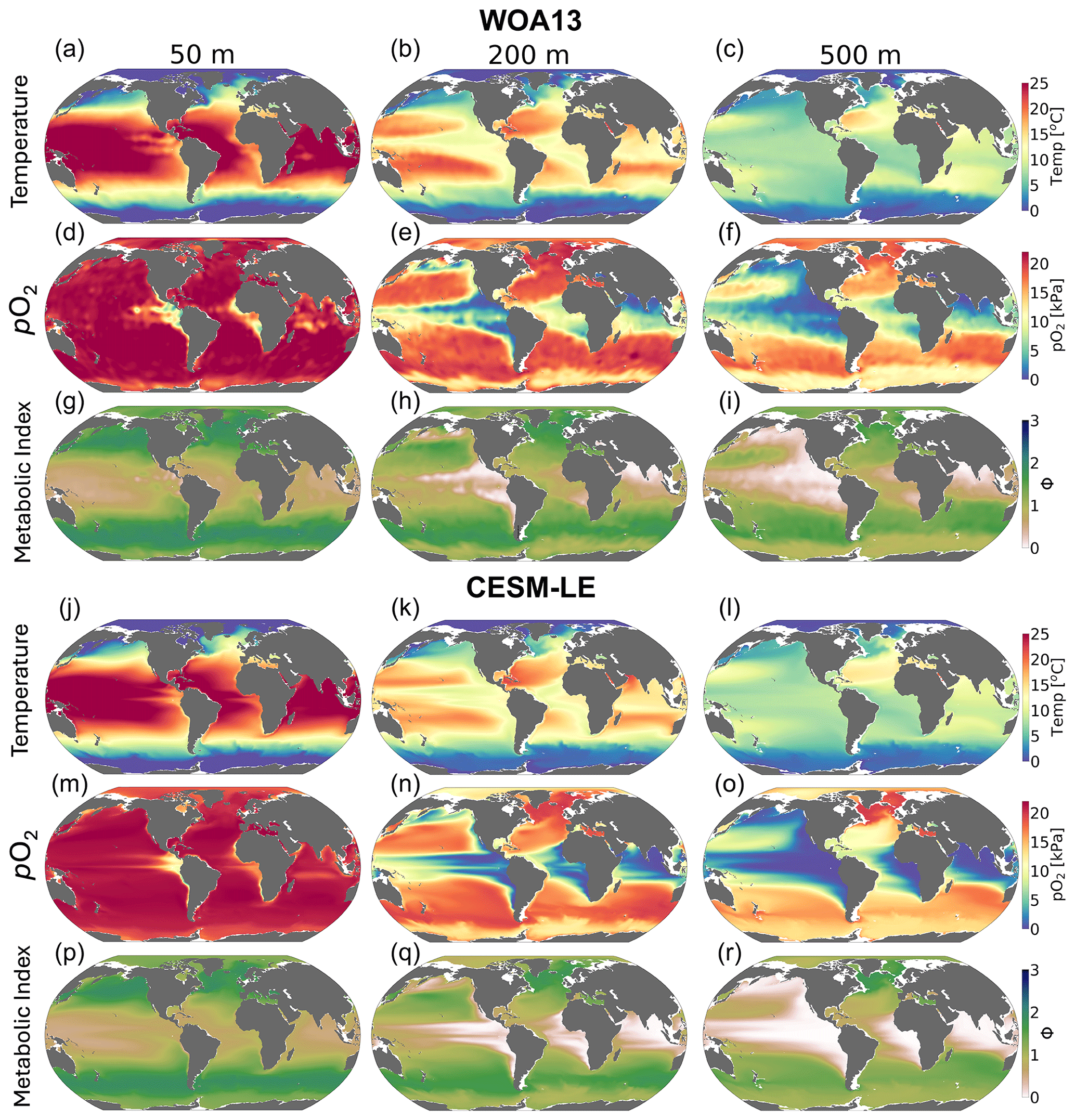
Figure 3 Mean-state comparison with observations. The climatological mean of (a–c, j–l) temperature (°C), (d–f, m–o) pO₂ (kPa) and (g–i, p–r) metabolic index for active metabolism (Φ^′) for the median ecotype (E_o=0.34, A_c=7.4); three depths are shown: (a, d, g, j, m, p) 50 m, (b, e, h, k, n, q) 200 m and (c, f, i, l, o, r) 500 m. Panels (a–i) show the WOA13 dataset, and panels (j–r) show CESM1-LE.

Table 1 Summary statistics for the comparison of CESM1-LE with the World Ocean Atlas dataset (Garcia et al., 2014). The columns include the mean bias, pattern correlation coefficient (PCC) and root mean square error (RMSE) at 50, 200 and 500 m.

3 Results

3.1 Joint temperature–pO₂ natural variability and forced trends

The spatial distribution of the number of viable ecotypes is shown in Fig. 4 for the “unperturbed” climate (1920–1965). Our intention here is not to quantify the actual biogeographic range of organisms in the environment but rather to illustrate the ocean's ability to support respiration by marine ectotherms given the metabolic capacities afforded within the trait space of extant organisms. High-latitude environments do not impose strong aerobic constraints (cold-intolerance notwithstanding); thus, over much of the Southern Ocean, North Atlantic and Arctic Ocean, almost all 61 ecotypes can sustain respiration. The tropical oceans impose the strongest aerobic constraints, restricting the viability of ecotypes that do not have a high hypoxia tolerance (A_o). For example, less than 25 ecotypes are viable over much of the tropical surface ocean (Fig. 4a); low concentrations of oxygen at depth impose even stronger constraints, and no ecotypes are viable in the core of OMZs (Fig. 4b and c). The spatial patterns of the number of viable ecotypes are tightly controlled by temperature at the surface since pO₂ is mostly near saturated levels; at depth, however, pO₂ is the dominant driver of geographic patterns in ecotype viability (Figs. 2–4). Temperature generally decreases with depth, reducing the metabolic oxygen demand. However, since pO₂ also decreases with depth and displays greater lateral heterogeneity, pO₂ emerges as the dominant constraint of spatial structure in ecotype viability at depth.

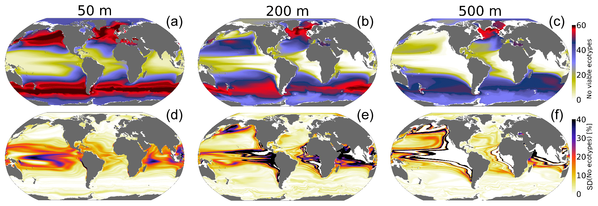
Figure 4 Metabolic constraints on trait–space viability. (a–c) The number of ecotypes from the physiological trait database that are viable (total=61) in the CESM1-LE over the period 1920–1965. (d–f) The standard deviation (expressed as a percent of the mean) in the number of viable ecotypes, reflecting fluctuations driven by natural variability.

The standard deviation of annual anomalies using all CESM1-LE ensemble members provides insight into the amplitude of natural variability (Fig. 5, 1 standard deviation). Temperature and pO₂ show similar patterns of natural variability in the upper ocean, both showing particularly large variance in the western tropical Pacific and Indian Ocean (Fig. 5a and d). Spatial variation in the magnitude of temperature variability generally decreases with depth, but pO₂ displays relatively larger variability at depth with respect to the surface in some regions (Fig. 5a–f). The joint pO₂–temperature variability manifests in variations of Φ^′ (Fig. 5g–i). Natural variability in Φ^′ computed for the median ecotype shows spatial patterns similar to those of temperature in the upper-surface ocean (50 m), but it is more similar to pO₂ at depth. Thus, variations in Φ^′ tend to be temperature-dominated near the surface but are more strongly controlled by pO₂ variability at depth. Φ^′ also shows the most extensive natural variability at 200 m, consistently with the variability of pO₂. The number of viable species shows more dramatic fluctuations than variations in the median-ecotype Φ^′; variations in the number of viable ecotypes exceed 30 % on annual timescales in the tropical upper ocean and near OMZ boundaries in the water column (Fig. 4c and d). This reflects the fact that interannual variability can preclude habitability for some regions of the A_c–E_o trait space, but these variations do not necessarily impact viability for the median ecotype (Fig. 1). In the tropical surface ocean, high temperatures (>25 °C) and saturated surfaces (pO₂>20 kPa) require a high hypoxia tolerance (A_c) but permit a range of E_o values (Figs. 1b, 2a and b). Ecotypes with larger temperature sensitivity (high E_o) are particularly responsive to variations in temperature.

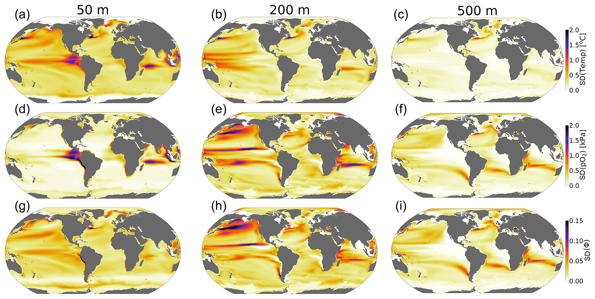
Figure 5 The amplitude of natural variability in the ocean's metabolic state. The panels show the standard deviation of the annual-mean anomalies of all ensemble members over the period 1920–1965 for (a–c) temperature (°C), (d–f) pO₂ (kPa) and (g–i) the metabolic index (unitless) of the median ecotype (E_o=0.34, A_c=7.4).

CESM1-LE simulates nearly homogeneous warming between 1920–1965 and 2070–2099 in the surface ocean (50 m) under RCP8.5, with an exception being the so-called North Atlantic warming hole (Fig. 6a). Both modeling and observational studies have linked the North Atlantic warming hole to the slowing of the Atlantic overturning circulation with climate change (Keil et al., 2020). The magnitude of ocean warming generally diminishes with depth except in the North Atlantic, where, despite reductions, the overturning circulation effectively propagates anthropogenic heat anomalies into the ocean interior. pO₂ shows heterogeneous changes between 1920–1965 and 2070–2099 (Fig. 6d–f). In the upper ocean, pO₂ changes are generally small (<1 kPa) because the near-surface is kept close to saturation via photosynthetic oxygen production and air–sea equilibration. At depth, however, pO₂ shows long-term changes linked to the accumulated effects of respiration and changes in circulation (Ito et al., 2017). At 200 m for example, the Pacific Ocean displays a basin-wide mean reduction in pO₂ of 2 kPa (∼30 %), while the Atlantic and Indian basins gain about >2 kPa (∼10 %–35 %) by the end of the century. The largest long-term pO₂ loss (>3 kPa) occurs in the North Pacific, while the largest pO₂ gain (∼2 kPa) occurs in the North Atlantic gyre and western Indian Ocean (Fig. 6e and f).

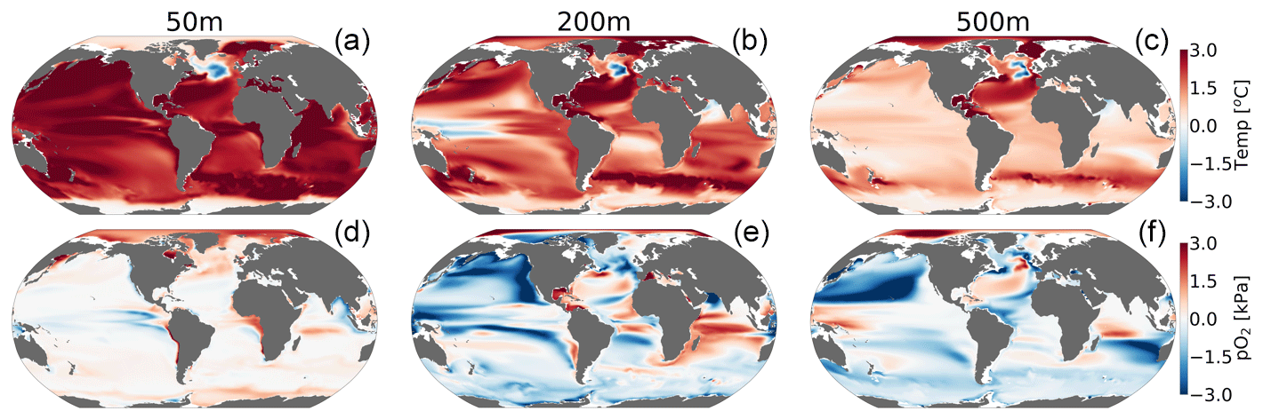
Figure 6 Net long-term change (2070–2099 minus 1920–1965) in the CESM1-LE ensemble mean temperature (a–c) and (d–f) pO₂ at 50, 200 and 500 m.

Figure 7 shows the relationship between interannual variations in pO₂ versus temperature (pO₂-T) in the unperturbed climate (1920–1965; top row) and for the forced trend associated with 21st-century climate change (2070–2099 minus 1920–1965; bottom row). The nature of the pO₂–T relationship is an important indicator of the impacts of variability on the metabolic state. Furthermore, the extent to which the forced trend is characterized by a pO₂–T relationship that is distinct from that associated with natural variability provides insight into the potential for advanced or delayed detection of signals in Φ relative to pO₂ or temperature alone. Given that metabolic rates for most organisms increase with temperature (positive E_o), a positive correlation between variations in temperature and pO₂ is generally indicative of compensating changes, wherein increased oxygen demand is at least partially offset by increased supply. Anticorrelation between temperature and pO₂, by contrast, will generally be associated with compounding impacts on the metabolic index as a negative correlation indicates that reductions in pO₂ (i.e., oxygen supply) accompany warming (i.e., increased demand). The sign of the pO₂–T relationship in the natural climate varies regionally and with depth (Fig. 7, top row). The surface ocean is generally characterized by a weak, positive pO₂–T relationship, which could manifest from, among other mechanisms, temperature-induced increases in photosynthetic oxygen production (Fig. 7a). The natural pO₂–T relationship in the epipelagic region (200 m) is characterized by strong positive correlations in the tropics and negative correlations at high latitudes (Fig. 7b). A positive correlation between pO₂ and temperature at this depth could be induced by variability associated with adiabatic vertical displacement of isopycnals or “heave”, which has the effect of translating background gradients in properties vertically in the water column (Long et al., 2016). Upward movement of a deep isopycnal surface would yield a negative temperature anomaly and a negative pO₂ anomaly (positive correlation) as the deeper, colder waters have greater oxygen utilization signatures associated with longer ventilation ages. Negative correlations between pO₂ and temperature could manifest from ventilation processes, where enhanced subduction of surface water yields anomalously cold water masses that are enriched in oxygen. The sign of these epipelagic pO₂–T correlations shows some similarity to that associated with the externally forced climate (Fig. 6e), but the latter is characterized by a greater prevalence of anticorrelation, most notably in the North Pacific Ocean. At 500 m depth, the relationship between temperature and pO₂ in the natural climate is almost a mirror image of the epipelagic region (Fig. 7c); the tropics generally display negative correlations, while polar regions show positive correlations (Fig. 7e). The pO₂–T relationship in the forced trend at 500 m is dominated by broad regions of deeply negative correlations, with the most pronounced effect again being in the North Pacific. The negative relationship is consistent with a ventilation signal as buoyancy-induced stratification from warming curtails the introduction of new oxygen into the ocean interior. The predominantly negative pO₂–T relationship associated with the forced trend is indicative of the compounding effects of climate change on metabolic state, increasing metabolic demand while simultaneously reducing oxygen supply.

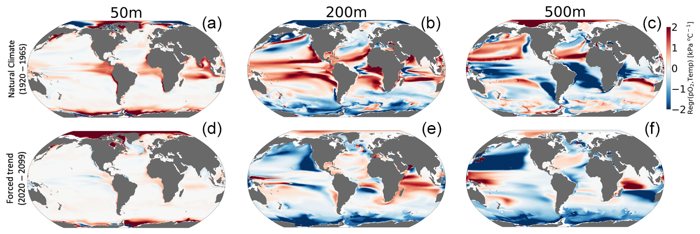
Figure 7 Regression of annual means pO₂ versus temperature (kPa °C⁻¹) for (a–c) interannual variability and (d–f) the forced trend (difference between 2020–2099 and 1920–1965). The columns show the regressions computed at different depths of 50 m (a, d), 200 m (b, e) and 500 m (c, f).

3.2 Long-term habitat changes

Figure 8 shows the climate-driven changes in Φ^′ for the median ecotype, as well as the impacts of climate change on the number of viable ecotypes. Notably, while pO₂ in the near-surface ocean is relatively insensitive to climate change (Fig. 6d), there are reductions in Φ^′ in the tropics (Fig. 9d) owing to the direct impacts of warming. These changes are associated with deep reductions in the number of viable ecotypes in the tropics (Fig. 8a). There are modest increases in Φ^′ and ecotype viability at high latitudes; metabolic state in these regions is affected by cold intolerance, and, thus, warming broadens the viable region of trait space. Additionally, sea ice melt supports an increase in pO₂ as gas exchange becomes more effective at restoring equilibrium oxygen concentrations. The number of viable ecotypes shows more intense patterns than those in the median-ecotype Φ^′ in the upper ocean (Fig. 8). This is partly because ecotypes predicted to lose viability in the tropical regions (∼50 %) are at the extremes of the A_c-E_o distribution (Fig. 1) and are not captured by the median-ecotype Φ^′. Nevertheless, outside the tropical regions, the median ecotype gives a good indication of the anthropogenic impact on marine ectotherms. The projected habitat loss in the epipelagic–pelagic North Pacific (>50 %) and habitat gain in the epipelagic–pelagic Southern Indian Ocean (∼40 %) and pelagic western tropical regions (∼40 %) are consistent with a decrease in the median-ecotype Φ^′. Note that the most pronounced effects on habitat are associated with regions where climate change drives a strongly negative pO₂–temperature relationship (Fig. 7).

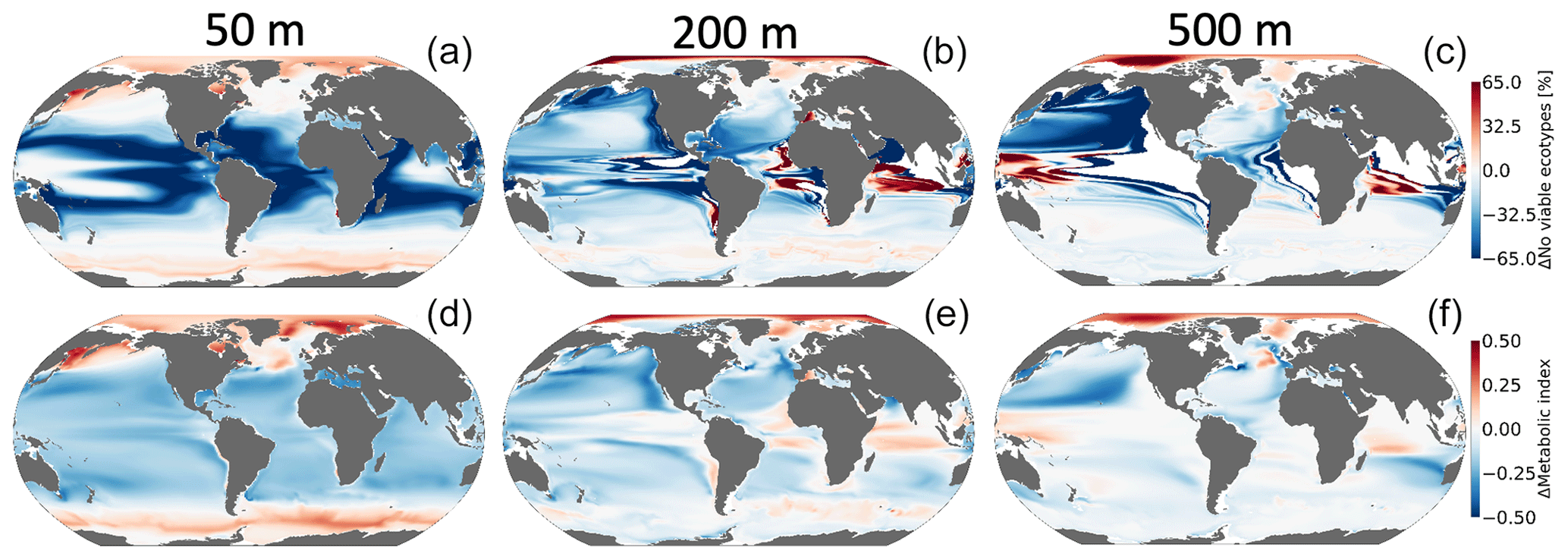
Figure 8 Net change in the number of habitable ecotypes in percentage (a–c). Net metabolic index change (2070–2099 vs. 1920–1965) for the median ecotype [E_o=0.34, A_c=7.4] (d–f) at 50 m (a, d), 200 m (b, e) and 500 m (c, f).

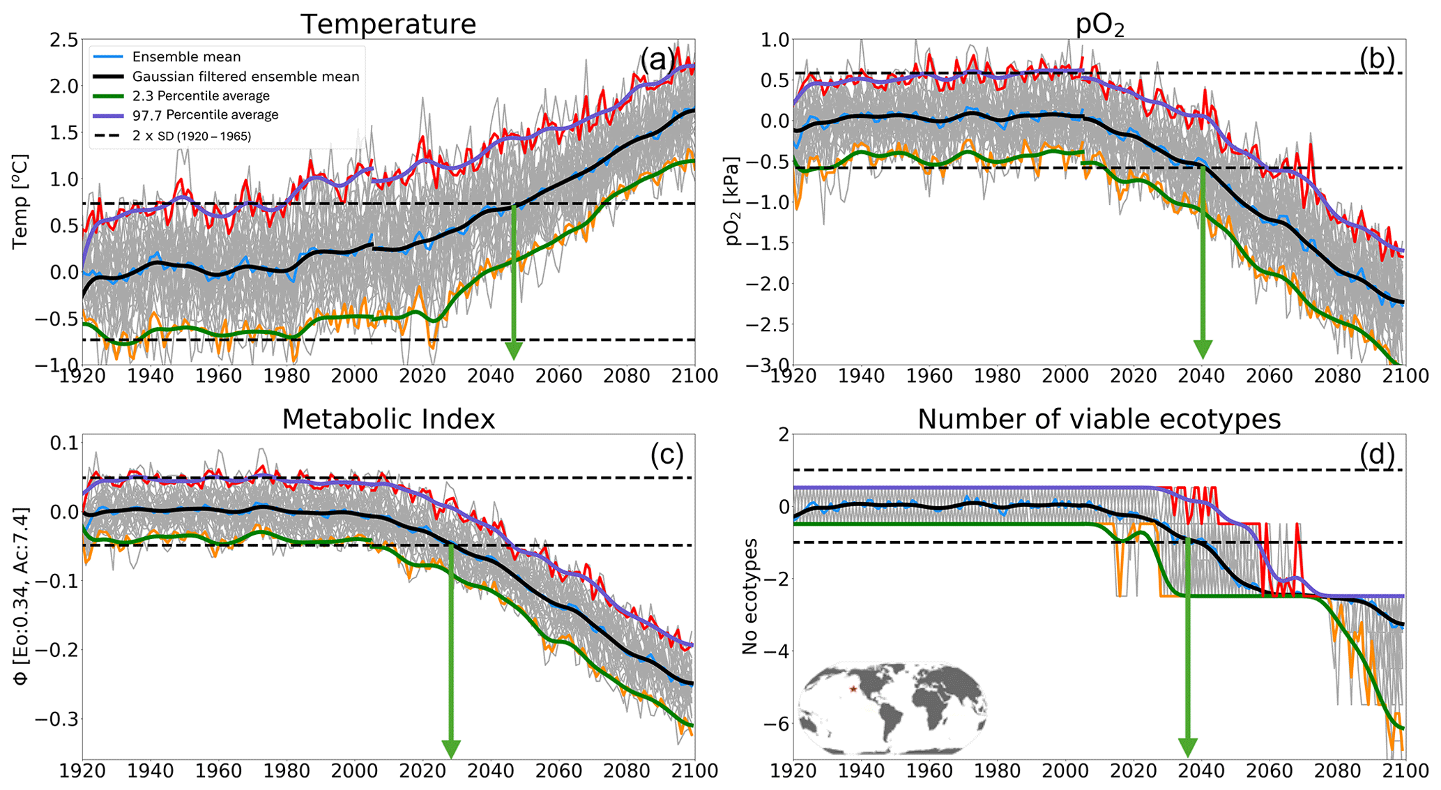
Figure 9 Time of emergence (ToE) of the climate forcing signal for (a) temperature, (b) pO₂, (c) the metabolic index of the median ecotype [E_o=0.34, A_c=7.4] and (d) the number of viable ecotypes for a single model grid in the North Pacific at 200 m. ToE (green arrows) is defined as the time when the forced trend signal (ensemble member time series) is above 2 standard deviations (dotted black line) compared to all ensemble members for the period 1920–1965.

3.3 Time of emergence

In this section, we examine the time of emergence (ToE, Hawkins and Sutton, 2012), the point when forced changes in pO₂, temperature and Φ^′ can be distinguished from the background natural variability. We define ToE as the time when the magnitude of change in the ensemble mean of a particular variable exceeds 2 standard deviations of the natural climate (1920–1965). This is illustrated in Fig. 9 for a single grid point in the North Pacific at 200 m. At this location, the forced trend in temperature shows a monotonic increase, while pO₂ shows a monotonic decrease; as a result, Φ^′ for the median ecotype and the number of viable ecotypes decrease over time. The anti-correlation between pO₂ and temperature exacerbates trends in Φ^′, and, hence, the forced trend of the median-ecotype Φ^′ emerges from natural noise earlier than either pO₂ or temperature do alone (Fig. 10a–c). Note that, although the ToE of ecotype viability change is directly derived from changes in Φ^′, it is binary-counted; changes in ecotype viability are counted in whole numbers, and this creates a step-function temporal–spatial variation (Fig. 9d). Consequently, this step-function-like feature of ecotype viability creates discontinuities, even in spatial patterns of ToE (Fig. 10j–l), as also shown in the natural variance in Fig. 4d–f.

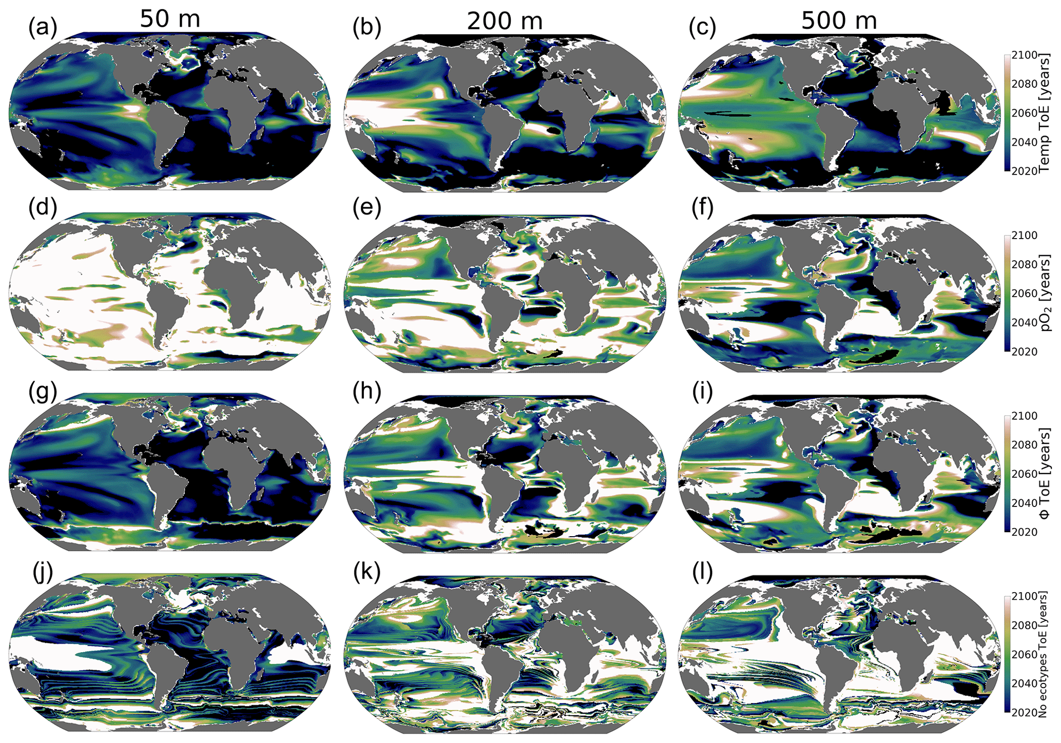
Figure 10 Time of emergence (ToE) of the climate forcing signal for temperature, pO₂, ϕ and the number of viable ecotypes. ToE is defined as the time when the forced trend signal (ensemble member time series) is above 2 standard deviations compared to all ensemble members for the period 1920–1965.

The ToE values of pO₂ and temperature are inverted with depth; temperature emerges earliest in the upper ocean, while pO₂ emerges earlier at depth, while in the upper ocean, it emerges later or shows no emergence (Fig. 10a–f). This feature is consistent with larger long-term upper-ocean temperature changes and greater pO₂ changes at depth. Near-surface ocean temperature is shown to have mostly already emerged by 2020 and is predicted to have almost completely emerged by the late 2060s under RCP85 (Fig. 10a–c). The early emergence of temperature from natural noise also persists for regions of relatively low natural variance at depth, e.g., the Southern Ocean and Atlantic basin gyres. However, regions of the largest natural variability (see Fig. 5) like the subtropical–subpolar Pacific do not emerge until close to the end of the century. For pO₂, anthropogenic changes in the upper ocean generally do not emerge from natural noise before the end of the century, except for the Arctic Ocean and eastern Antarctic. In the Arctic Ocean and eastern Antarctic, pO₂ gain is related to sea melt emergence by the mid-2050s (Fig. 10a). The median-ecotype Φ^′ ToE shows spatial patterns that are coherent with temperature ToE in the upper ocean, with the exception of polar regions. In contrast, these are consistent with pO₂ ToE patterns at depth; this is consistent with net long-term Φ^′ changes in Fig. 9d. The emergence of the anthropogenic signal in ecotype viability closely resembles the median-ecotype Φ^′ spatial patterns but with non-harmonious spatial patterns due to the step-function-like counting feature of viability changes. It shows that the predicted ∼50 % ecotype viability loss in the tropics (Fig. 6a) may already be distinguishable from natural variability by the mid-2030s. In the North Pacific, the predicted >50 % ecotype viability loss in the epipelagic–pelagic regions is predicted to start emerging in the 2040s at 500 m and in the 2080s at 200 m (Fig. 10k and l).

In summary, we showed that, because of the surface ocean’s large warming signal and the lowest pO₂ loss outside of the polar regions in the RCP85 climate scenario, the surface ocean is characterized by habitat loss in the tropics and a slight habitat gain in the polar regions (Fig. 11). Sea ice melt supports oxygen gain through the enhancement of temperature-driven solubility in the surface polar regions. At depth, warming is less prevalent by the end of the 21st century; however, oxygen loss related to the weakening ventilation of the ocean interior as the ocean becomes more stratified has a stronger impact on metabolic reliance, leading to habitat loss in the tropics and subtropics. On the other hand, cooler temperatures and efficient ventilation in polar regions create an oxygen-rich environment. Thus, in contrast to tropical and subtropical regions, warming leads to a slight habitat gain (Fig. 11) as organisms escape the cold intolerance imposed by molecular gas diffusion at low temperatures.

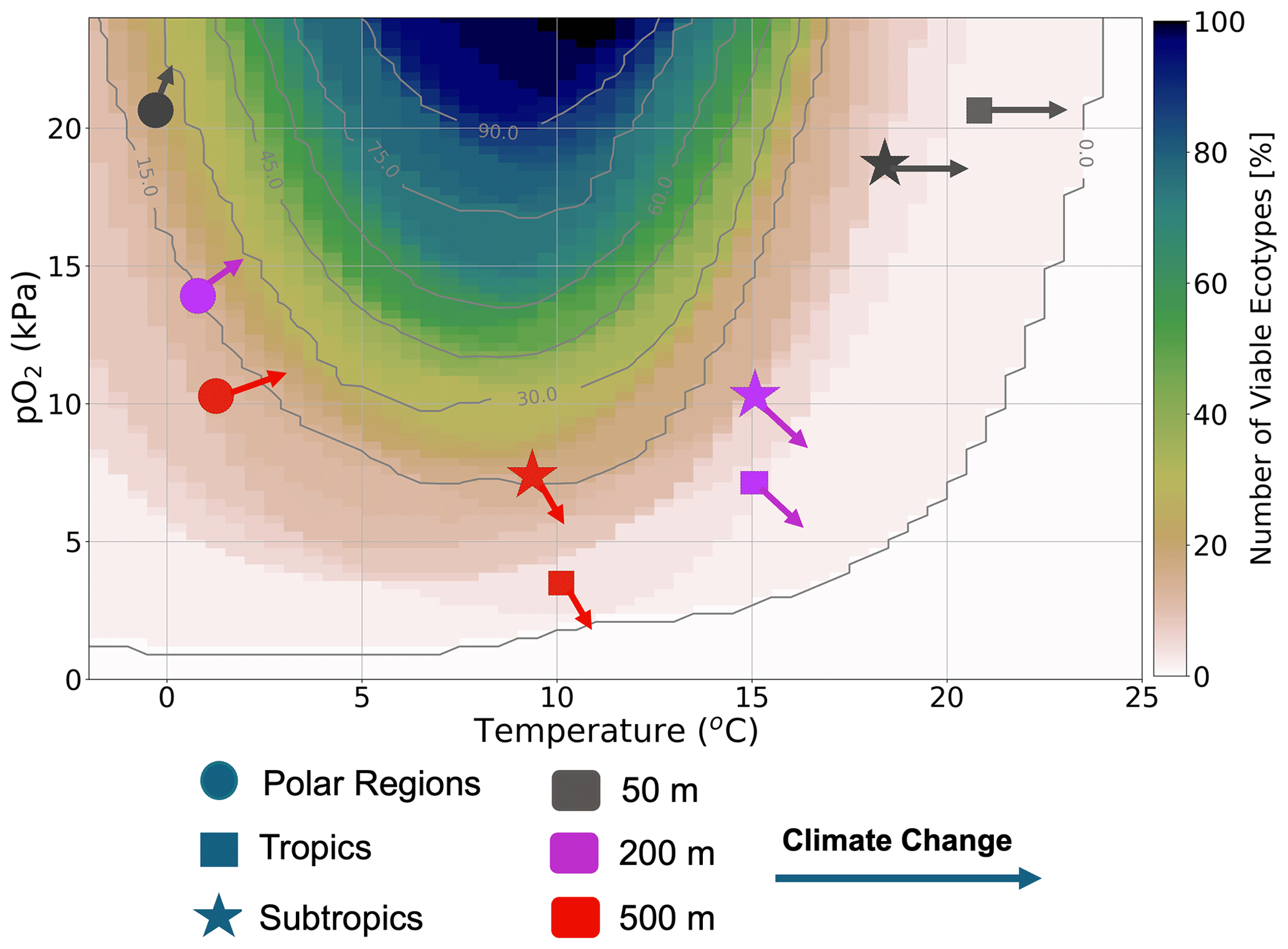
Figure 11 Summary figure: the distribution of ecotype viability within representative ocean temperature and pO₂ boundaries for the 66 species analyzed in this study. The markers represent the subsampled regions, with polar regions denoted by circles, tropical regions denoted by squares and subtropical regions denoted by stars. The colors represent the depth levels; 50 m (gray), 200 m (purple) and 500 m (red). Each arrow shows the estimated joint temperature–pO₂ climate change vector based on the net changes in temperature and pO₂ (as depicted in Fig. 6).

4 Discussion

The human-induced rapid warming of the planet has been shown to drive ocean deoxygenation (Ito et al., 2017; Schmidtko et al., 2017; Long et al., 2016). Higher metabolic oxygen demand at higher temperatures (Gillooly et al., 2001; Deutsch et al., 2015, 2022) raises concerns about the ability of marine ectotherms to support aerobic respiration in the future. This study set out to characterize the anticipated climate change signal in the ocean's metabolic state in the context of natural variability using metabolic theory as a basis to examine the capacity of the environment to support ectothermic marine heterotrophs.

The spatial variation in pO₂ and temperature in the unperturbed natural climate state set biogeographic boundaries based on ectotherms' physiological performances. The resilience of these ectotherms' biogeographic structures to natural variability and long-term climate warming is perturbed by the joint pO₂–temperature changes, effectively measured by the metabolic index (Φ^′). An increase in the capacity of the organisms to support aerobic respiration increases Φ^′ – for example, by ocean cooling or increases in oxygen supply. On the contrary, ocean warming and decreases in oxygen supply decrease Φ^′. There are exceptions in extremely low-temperature environments (Fig. 11), where aerobic respiration is also limited by kinematic gas transfer into the organism in addition to environmental oxygen supply. Relative changes in pO₂ and temperature in the natural variability and forced trend therefore regulate ectotherms' resilience to environmental changes. Under the RCP85 climate scenario, the ocean generally warms homogeneously, but concurrent pO₂ changes are heterogeneous and vary with depth. Thus, the characteristics of these pO₂–temperature forced trend changes determine when the climate change impact on marine ectotherms can be distinguishable from natural variability.

In the surface ocean, pO₂ is generally abundant and relatively uniform; thus, spatial temperature variations have a dominant constraint on the spatial variations of the organismic metabolic state. The warmest parts of the surface ocean, the tropical oceans, can only support about 10–20 (∼30 %) of the 61 ecotypes, while cooler regions in the extra tropics have nearly 100 % viability. Moreover, since warming anomalies propagate from the surface, the surface tropical oceans also show the largest natural variance in temperature and ecotype viability. This is because extremely warm temperatures in the surface tropics (>25 °C) are mainly suited for organisms with a high temperature sensitivity (E_o), which are relatively fewer and are mostly close to their physiological limits (Storch et al., 2014). Large natural variability in the warmest parts of the tropical surface ocean precludes the forced trend signal from emerging from the natural variability in the ecotype viability by end of the century, although the ocean warms the most at the surface. Nevertheless, the large warming trends in the surface ocean generally emerge relatively early (the 2020s) from natural variability in both temperature and ecotype viability in most regions. Minimal changes in surface pO₂ in the forced trend affirm that surface ocean marine ectotherms are mainly perturbed by temperature in the context of anthropogenic changes. In polar regions, warming has a counterintuitive effect on marine ectotherms with respect to most parts of the surface ocean. There, warming helps organisms escape extreme cold intolerances by enhancing membrane kinematic gas transfer, which enhances Φ^′ and thus ecotype richness in the future (Fig. 11)

In the epipelagic and mesopelagic regions (200 and 500 m), the forced temperature trend and natural variability are broadly smaller than the surface ocean, while pO₂ changes show the opposite. Thus, at depth, pO₂ plays a more intricate role in perturbating marine ectotherm habitats in the context of anthropogenic warming with respect to the surface ocean, where temperature plays a dominant role. Contrasting the regression between pO₂ and temperature in the natural climate, forced trends provide an instructive framework to analyze ectotherms' long-term changes. Regions showing different correlations between temperature and pO₂ in the forced trends in comparison to the natural climate suggest a loss of metabolic resilience and a loss of habitat, and these regions tend to have a relatively early ToE values. For instance, in the epipelagic and mesopelagic North Pacific, temperature–pO₂ regressions switched from a positive correlation in the unperturbed climate to a strong negative correlation in the forced trend (Fig. 7). The North Pacific pelagic–epipelagic region is projected to lose nearly half of the present climate ecotype viability by the end of the 21st century, with the projected habitat loss starting to emerge by the late 2030s under the RCP85 climate scenario. On the other hand, in the Arctic Ocean and some parts of the Southern Ocean, same-sign pO₂–temperature correlations in the forced trends result in the preservation of the marine habitat and even slight enhancements.

5 Conclusions

The joint temperature–oxygen metabolic framework in this study provides additional insights into the impact of climate change on marine ecosystems in comparison to the independent oxygen or temperature analysis. Here, we showed that, while warming is the leading-order driving mechanism of climate change, the direct effect of warming on marine ecosystems is mostly in the upper ocean. Climate-change-related oxygen loss is a major driver of marine ecosystem stress in addition to warming at depth. Incorporating organismal physiological sensitivity to oxygen–temperature changes in the metabolic framework provides insights into how climate impacts the biogeographic structure of marine habitats. We find that forced perturbations to pO₂ and temperature will strongly exceed those associated with the natural system in many parts of the upper ocean, mostly pushing organisms in these environments closer to or beyond their physiological limits. Climate warming is expected to drive significant marine habitat loss in the surface tropical oceans and epipelagic–pelagic North Pacific basin while gaining marginal habitat viability in the surface Arctic Ocean and some parts of the Southern Ocean.