Influence of wind strength and direction on diffusive methane fluxes and atmospheric methane concentrations above the North Sea

Quantification of the diffusive methane fluxes between the coastal ocean and atmosphere is important to constrain the atmospheric methane budget. The determination of the fluxes in coastal waters is characterized by a high level of uncertainty. To improve the accuracy of the estimation of coastal methane fluxes, high temporal and spatial sampling frequencies of dissolved methane in seawater are required, as well as the quantification of atmospheric methane concentrations, wind speed and wind direction above the ocean. In most cases, these atmospheric data are obtained from land-based atmospheric and meteorological monitoring stations in the vicinity of the coastal ocean methane observations.

In this study, we measured wind speed, wind direction and atmospheric methane directly on board three research vessels in the southern North Sea and compared the local and remote atmospheric and meteorological measurements on the quality of the flux data. In addition, we assessed the source of the atmospheric methane measured in the study area in the German Bight using air mass back-trajectory assessments.

The choice of the wind speed data source had a strong impact on the flux calculations. Fluxes based on wind data from nearby weather stations amounted to only 58 ± 34 % of values based on in situ data. Using in situ data, we calculated an average diffusive methane sea-to-air flux of 221 ± 351 µmol m⁻² d⁻¹ (n = 941) and 159 ± 444 µmol m⁻² d⁻¹ (n = 3028) for our study area in September 2019 and 2020, respectively. The area-weighted diffusive flux for the entire area of Helgoland Bay (3.78 × 10⁹ m²) was 836 ± 97 and 600 ± 111 kmol d⁻¹ for September 2019 and 2020, respectively. Using the median value of the diffusive fluxes for these extrapolations resulted in much lower values compared to area-weighted extrapolations or mean-based extrapolations.

In general, at high wind speeds, the surface water turbulence is enhanced, and the diffusive flux increases. However, this enhanced methane input is quickly diluted within the air mass. Hence, a significant correlation between the methane flux and the atmospheric concentration was observed only at wind speeds < 5 m s⁻¹.

The atmospheric methane concentration was mainly influenced by the wind direction, i.e., the origin of the transported air mass. Air masses coming from industrial regions resulted in elevated atmospheric methane concentrations, while air masses coming from the North Sea transported reduced methane levels. With our detailed study on the spatial distribution of methane fluxes we were able to provide a detailed and more realistic estimation of coastal methane fluxes.

1 Introduction

1.1 Necessity for coastal methane data

Methane (CH₄) is the second-most important greenhouse gas (GHG) after carbon dioxide (CO₂), accounting for 16 %–25 % of atmospheric warming to date (Etminan et al., 2016). Aquatic ecosystems contribute 41 % (median) or 53 % (mean) of total global CH₄ emissions from anthropogenic and natural sources (Rosentreter et al., 2021a). Coastal seas are an important global source of GHGs (Saunois et al., 2020). For the open and coastal ocean, including estuaries, Saunois et al. (2020) suggested an emission of 6 (range 2–10) Tg CH₄ yr⁻¹. A more recent study from Rosentreter suggested an emission of 8.4 (4.8–28.4, Q₁–Q₃) Tg CH₄ yr⁻¹, with a contribution of 3 % from estuaries, 13 % from tidal flats and 52 % from continental shelves (Rosentreter et al., 2021a). The near-shore environments hence contribute the largest but most uncertain diffusive fluxes despite accounting for only ∼ 3 % of the global ocean area.

The reasons for the large range of and uncertainty in coastal CH₄ fluxes are associated with the high spatial and temporal variability of fluxes in coastal ecosystems, driven by, for example, variations in tidal pumping and salinity gradients (Rosentreter et al., 2021a), exacerbated by a paucity of data with sufficient temporal and spatial resolution (Weber et al., 2019). Overall, aquatic GHG emissions are causing considerable uncertainty in global GHG assessments (Pörtner et al., 2021). Thus, reducing the uncertainty in aquatic GHG budgets is important to allow for improvements to biogeochemical models and climate predictions.

1.2 Traditional method for flux calculation

The air–sea gas flux is a function of the gas transfer velocity (k) and atmospheric and oceanic CH₄ concentrations (Wanninkhof, 2014; see the “Material and methods” section for details). Since k is difficult to measure, it is often parameterized using widely measured parameters such as wind speed. In offshore regions with greater water depth, wind is known as a good predictor of the gas transfer velocity because wind creates waves and currents, which control turbulence and bubbles at the sea surface (Wanninkhof et al., 2009). In shallow waters, k can also be well estimated by wind speed when the water depth is more than 10 m (Ho et al., 2018). Other techniques to determine k are eddy covariance measurements, tracer injection methods (Gutiérrez-Loza et al., 2022; Dobashi and Ho, 2023) and chamber measurements (Rosentreter et al., 2021b). The best way to determine k is an ongoing matter of debate.

Diffusive CH₄ fluxes are typically determined from direct surface ocean CH₄ observations and parameterizations of wind speed and atmospheric CH₄ concentrations. The atmospheric data used are normally taken from coastal meteorological stations in close proximity to the marine observations (see for example Myllykangas et al., 2020; Woszczyk and Schubert, 2021), or a combination of in situ data and data obtained from a meteorological station is used (Mau et al., 2015; Bussmann et al., 2021b; Humborg et al., 2019). Other studies use in situ data for all variables (de Groot et al., 2023; Thornton, 2016, no. 2655). We are not aware of any study on the influence of the data source on the quantification of diffusive CH₄ fluxes.

1.3 Atmospheric methane above a water body

The atmospheric CH₄ concentration is determined by several factors. One is the sea-to-air transfer through the diffusive CH₄ flux (Wanninkhof, 2014), implying that periods or areas with high diffusive CH₄ fluxes into the atmosphere would result in higher atmospheric CH₄ concentrations. However, there are contrasting reports in the literature in marine science, with the highest atmospheric CH₄ concentrations being observed during cruises with the lowest CH₄ fluxes (Silyakova et al., 2020). Increasing atmospheric CH₄ levels were not found alongside enhanced dissolved CH₄ concentrations (Vogt et al., 2023; Law et al., 2010). These studies show that there is no clear mechanistic understanding of the relationship between dissolved CH₄ concentrations, CH₄ fluxes into the atmosphere and atmospheric CH₄ concentrations in shallow coastal water areas.

1.4 Methane in the North Sea

The CH₄ budget of the central North Sea is characterized by pockmarks (Römer et al., 2021), drilling activities (Vielstädte et al., 2017) and gas ebullition sites (Mau et al., 2015). In contrast, in the southern North Sea and areas close to the mainland, dissolved CH₄ mainly originates from autochthonous methanogenesis in sediments (Yin et al., 2019) with subsequent fluxes into the water column, tidal flats (Røy et al., 2008; Wu et al., 2015) and riverine inputs (Upstill-Goddard and Barnes, 2016). Borges et al. (2017) showed that warm summers in northern Europe in recent years have resulted in increased dissolved CH₄ concentrations due to enhanced methanogenesis, which has led to higher sea-to-air CH₄ fluxes along the Belgian coast (Borges et al., 2017, 2019).

Previous studies have investigated the temporal and spatial patterns of dissolved CH₄ between the German North Sea coast and the island of Helgoland (60 km offshore) on a monthly basis from 2010 to 2014 (Matousu et al., 2017; Osudar et al., 2015; Hackbusch et al., 2019). In these studies, the CH₄ concentrations near the coast ranged between 30 and 51 nmol L⁻¹, whereas near Helgoland, the concentrations were 14 ± 6 nmol L⁻¹. However, no flux data were calculated in these studies. At these high concentrations of dissolved CH₄ in the coastal North Sea (the equilibrium concentration is 2–3 nmol L⁻¹), the diffusive flux is mainly directed from the sea into the atmosphere.

1.5 Aim of study

The aim of this study was to establish the diffusive CH₄ fluxes from the sea into the atmosphere in the southern German Bight (North Sea) based on CH₄ concentration data of high spatial and temporal resolution. We also investigated the influence of the use of different auxiliary datasets on the calculation of the diffusive CH₄ fluxes over a wide area of Helgoland Bay. We assessed whether increased diffusive CH₄ fluxes lead to detectable increases in atmospheric CH₄ concentrations and identified the atmospheric factors that influence CH4 concentrations in a given area.

2 Material and methods

2.1 Study sites

The cruises Stern 3 and 5 were performed in September 2019 and 2020 as part of the Modular Observation Solutions for Earth Systems (MOSES; Weber et al., 2021) subproject of the Hydrological Extremes working group.

On Stern 3, the research vessel (RV) Littorina (German Helmholtz Centre GEOMAR), RV Ludwig Prandtl (German Helmholtz Centre Hereon) and RV Uthörn (German Helmholtz Centre AWI) left the harbor of Cuxhaven (Fig. 1) on 9 September 2019, heading for the island of Helgoland (German Bight) following different cruise tracks. On 10 September 2019, RVs Littorina and Ludwig Prandtl returned to Cuxhaven and the Elbe Estuary, while RV Uthörn returned via the Weser River to Bremerhaven (Bussmann et al., 2020).

For Stern 5, the three research vessels started from Cuxhaven and the Elbe Estuary on 30 August 2020, again heading for Helgoland (Fig. 2). In the following days, RV Littorina covered the area between Helgoland and Büsum (on the mainland), extending the cruise track towards the east. RV Ludwig Prandtl covered the area further north and west of the island of Amrum. RV Mya II (German Helmholtz Centre AWI) covered the area between Helgoland and Bremerhaven with the Weser Estuary. On the last day (3 September 2020), RV Mya II ended the cruise in Sylt, while the others returned to Cuxhaven (Bussmann et al., 2021a).

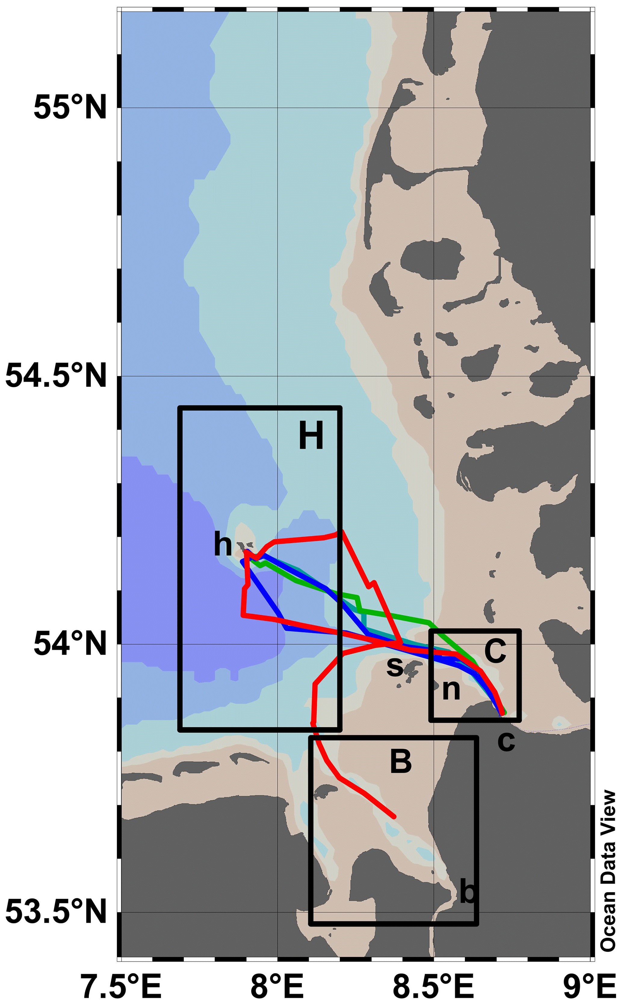
Figure 1 Cruise tracks for Stern 3 in September 2019 with RVs Littorina (blue), Ludwig Prandtl (green) and Uthörn (red). The areas for different flux calculations are also indicated: the area around Bremerhaven (B) with its meteorological station (b), the area around Cuxhaven (C) with its meteorological station (c) and the area around Helgoland (H) with its meteorological station (h). The islands Neuwerk (n) and Scharhörn (s) are also indicated. Schlitzer, Reiner, Ocean Data View, https://odv.awi.de, last access: 23 August 2024.

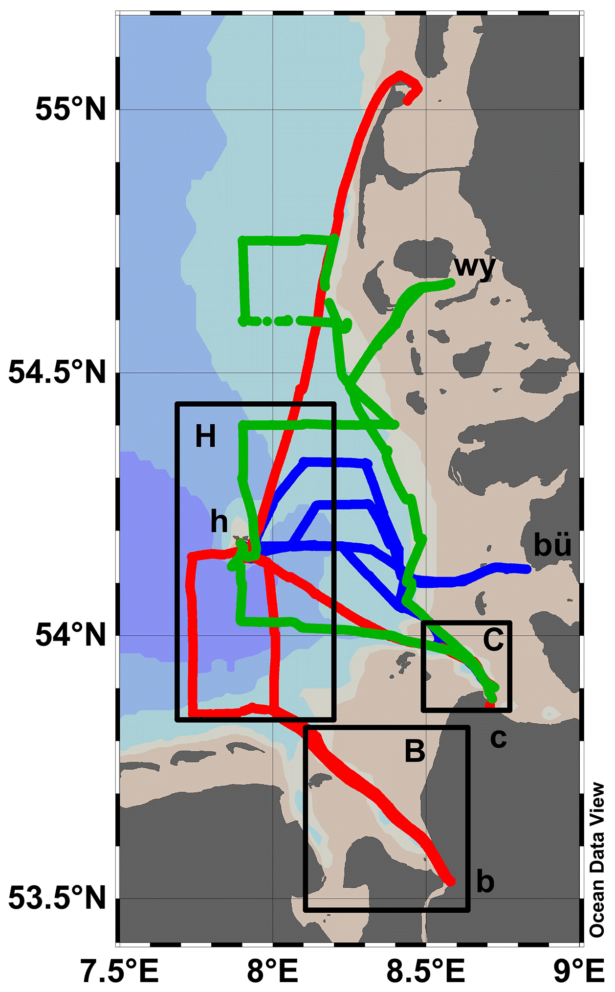
Figure 2 Cruise tracks for Stern 5 in September 2020 with RVs Littorina (blue), Ludwig Prandtl (green) and Mya II (red). The areas for different flux calculations are also indicated: the area around Bremerhaven (B) with its meteorological station (b), the area around Cuxhaven (C) with its meteorological station (c) and the area around Helgoland (H) with its meteorological station (h). The villages Büsum (bü) and Wyk auf Föhr (wy) are also indicated. Schlitzer, Reiner, Ocean Data View, https://odv.awi.de, last access: 23 August 2024.

2.2 Hydrographic and meteorological parameters

Basic hydrographic parameters, such as temperature, salinity, pH, oxygen, turbidity and chlorophyll fluorescence, were measured by shipboard measurement systems (FerryBoxes, 4H-Jena, Germany) on all ships. FerryBox systems had been checked and calibrated during routine maintenance and in preparation for the cruises (Petersen, 2014). The water supply to the FerryBoxes and CH₄ analyzers (see “Methane analysis” section below) was taken from the ships' underway surface water supply (intake at 1–2 m). The water from the ship was either pumped through a flow-through basin with ambient air pressure (Stern 3) or from a specific in situ pump tower (Stern 5) with a 10 L volume, pressure regulator and water overflow. Full details are in the cruise reports (Bussmann et al., 2020, 2021a). Both systems ensured a constant and sufficient surface water supply to all sensors.

True wind speed and true wind direction were provided by the DSHIP system (nautical data system, Werum) or equivalent systems of Ludwig Prandtl, Mya and Uthörn (no data were available from RV Littorina) with a frequency of 1 min⁻¹. Available wind speed data were corrected to U₁₀ (at 10 m height) with the respective measuring height (Touma, 1977):

$$\begin{array}{}\text{(1)}& U_{\mathrm{10}}=U_{\mathrm{ship}}{\left(\mathrm{10}/z_{\mathrm{ship}}\right)}^{\mathrm{0.143}}.\end{array}$$

For any further calculations, we used the rolling mean over 10 min. For comparison, we also used wind data (hourly means) provided by the German Meteorological Service (https://cdc.dwd.de/portal/, last access: 14 November 2022) for the Bremerhaven, Cuxhaven and Helgoland Dune weather stations. For each station, an area was set for which the respective wind data were used for the flux calculations (Figs. 1 and 2). Data on local tidal cycles were provided by the Bundesamt für Seeschifffahrt und Hydrographie (Federal Maritime and Hydrographic Agency, https://www.bsh.de/DE/DATEN/Vorhersagen/Gezeiten/gezeiten_node.html, last access: 8 June 2023) for the Büsum and Wyk auf Föhr sites.

2.3 Methane analysis

Dissolved CH₄ concentrations were measured with a dissolved gas extraction unit and a laser-based analytical greenhouse gas analyzer (GGA; both Los Gatos Research, United States) on all three ships. The degassing devices withdrew water from the flow-through units at 1.2 L min⁻¹. Methane was extracted from the water via a hydrophobic membrane and hydrocarbon-free carrier gas on the other side of the membrane (synthetic air or nitrogen, at 0.5 L min⁻¹). The carrier gas with the extracted CH₄ was then directed to the inlet of the gas analyzer. The time offset between the water intake and stable recording at the GGA was determined beforehand in the laboratory.

To convert the relative concentrations (ppm) given by the GGA to absolute concentrations (nmol L⁻¹), discrete water samples were obtained at least every hour. The CH₄ concentration in these bottles was determined using the headspace method and gas chromatographic analysis (Magen et al., 2014). Based on the obtained values, conversion factors (ppm to nmol L⁻¹) were determined for each setup. The regression lines and equations are given in the supplementary information (Fig. S1). Histograms for dissolved CH₄ concentrations are shown in Fig. S2. From the intercalibration stations (see “Data management and handling”) we calculated an instrumental error of 3.6 %. To test the lower sensitivity of the setup, aerated freshwater with an equilibrium concentration of 2.9 nM was measured in the laboratory, and the instrument readings gave a concentration of 2.3 ± 0.3 nM.

For quality control, the regional boundaries were set to 1–500 nmol L⁻¹ (see “Data management and handling”).

Atmospheric CH₄ was measured on board the following research vessels: for Stern 3 on the Littorina, Ludwig Prandtl and Uthörn with a Picarro G2301, a Picarro G2301 and a microportable greenhouse gas analyzer (Los Gatos), respectively; for Stern 5 with a Picarro G2301, a Li-Cor LI-8100A and another Picarro G2301, respectively. All data were corrected by the instruments for water vapor, resulting in CH₄ dry values. The inlets for the instruments were approximately 4 m above the water surface and located either at the ship's bow (Littorina) or on a railing on the bridge (other ships). For quality control, the regional boundaries were set to 1.8–2.3 ppm (see “Data management and handling”). Additional data for atmospheric CH₄ concentration were obtained from the meteorological station in Mace Head, Ireland (https://gml.noaa.gov/dv/data/index.php?site=MHD, last access: 21 August 2023), using the monthly means of September 2019 and September 2020 (1.942 and 1.957 ppm, respectively).

2.4 Calculation of the diffusive methane flux

The overall gas exchange across an air–water interface was determined according to Wanninkhof et al. (2009) as

$$\begin{array}{}\text{(2)}& F=k_{{\mathrm{CH}}_{\mathrm{4}}}\cdot \left(c_{\mathrm{m}}-c_{\mathrm{equ}}\right),\end{array}$$

where F is the rate of gas flux per unit area (µmol m⁻² d⁻¹), c_m is the measured CH₄ concentration of the surface waters and c_equ is the atmospheric gas equilibrium concentration (Wiesenburg and Guinasso, 1979). For the atmospheric CH₄ concentration data, we used either our measured data or the data from the Mace Head observatory.

The gas exchange coefficient (k) is a function of water surface agitation. The k value in oceans and estuaries is mostly determined by wind speed (U₁₀). The determination of k is crucial for calculating the sea–air flux. We calculated the gas exchange velocity k₆₀₀ according to the following equation for coastal seas (Nightingale et al., 2000):

$$\begin{array}{}\text{(3)}& k_{\mathrm{600}}=\mathrm{0.333}{U}_{\mathrm{10}}+\mathrm{0.222}{U}_{\mathrm{10}}^{\mathrm{2}}.\end{array}$$

We applied the wind-speed-based k₆₀₀ parameterization from Nightingale et al. (2000) here, largely because it is commonly used and represents a compromise between relationships that have a very strong or a very weak wind speed dependence (Yang et al., 2019).

The calculated k₆₀₀ (for CO₂ at 20 °C) was converted to $k_{{\mathrm{CH}}_{\mathrm{4}}}$ (Striegl et al., 2012), and the Schmidt number (Sc) was adjusted based on water temperature and salinity (Wanninkhof, 2014):

$$\begin{array}{}\text{(4)}& k_{{\mathrm{CH}}_{\mathrm{4}}}/k_{\mathrm{600}}={\left({\mathit{Sc}}_{{\mathrm{CH}}_{\mathrm{4}}}/{\mathit{Sc}}_{{\mathrm{CO}}_{\mathrm{2}}}\right)}^{-\mathrm{0.5}}.\end{array}$$

To determine the influence of wind and atmospheric CH₄ on the flux calculation, three combinations of datasets were applied (Table 1):

• flux 1 with in situ wind and in situ atmospheric CH₄ concentrations, with a resolution of 1 min;

• flux 2 with in situ wind but with the atmospheric CH₄ concentrations from the Mace Head station in Ireland, with a resolution of 1 month;

• flux 3 fixed monthly atmospheric concentration from the Mace Head station and using hourly wind data from the German Meteorological Service.

Table 1 Calculation of the diffusive CH₄ flux with several combinations of data sources.

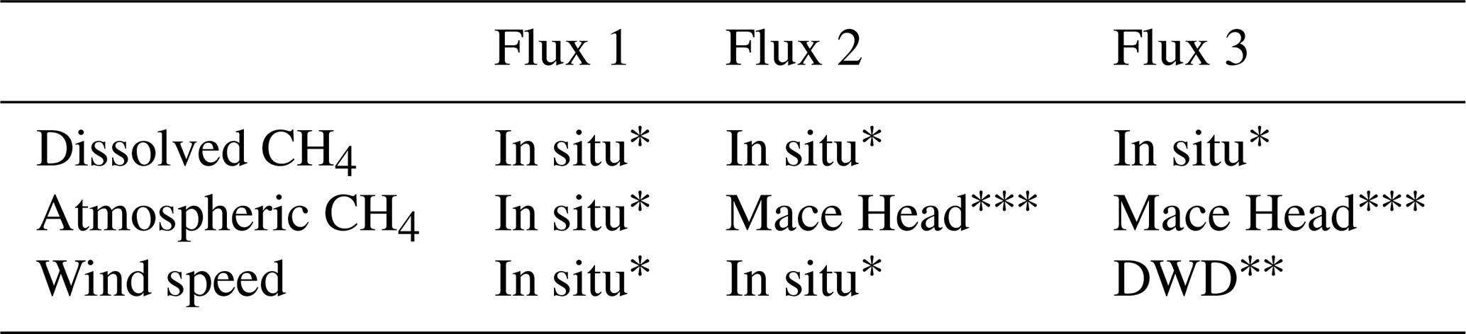
^* Temporal resolution of every minute, ${}^{**}$ every hour and ${}^{***}$ every month.

To improve the estimation of the diffusive CH₄ flux for the whole study area, we calculated an area-weighted diffusive flux. We split the diffusive flux data (flux 1 data, n = 941 for 2019 and n = 3028 for 2020) into groups with a bin size of 100 µmol m⁻² d⁻¹ and calculated a frequency distribution of the mean diffusive flux classes (0–100, 100–200, 200–300 µmol m⁻² d⁻¹, etc.). Next, the relative area was calculated by multiplying the relative frequency of each class by the total area. Then, the relative area of each class was multiplied by the respective diffusive flux to obtain the relative areal flux. The sum of all relative areal fluxes finally resulted in the total weighted flux of the whole area. The standard deviation was determined from the relative areal fluxes. An example of the calculation is given in Table S1 in the Supplement.

To enhance the validity of our results, we extrapolated our calculated diffusive fluxes from our respective study areas to areas in accordance with the ecosystem type classification of the German Federal Statistical Office (Statistisches Bundesamt; Destatis, 2021), which assigns all areas of Germany to different ecosystem types without gaps or overlaps (https://oekosystematlas-ugr.destatis.de/, last access: 3 July 2023). We used the following ecosystems, overlapping with our cruise track: the eastern Wadden Sea of the Weser River (490000003), the open coastal sea of the Weser (490000004), the coastal sea of the Weser (490000005), Helgoland (590000002), the coastal sea of the Elbe River (590000003), the western Wadden Sea of the Elbe (590000005), outer Elbe north (590000006) and the Piep tidal basin (950000001, Fig. S3). These ecosystems cover a total area of 3.78×10⁹ m² (377947 ha).

2.5 Data management and handling

During the cruises or shortly afterwards, all data from all ships were uploaded to AWI's data web service (Koppe et al., 2015; https://ingest.o2a-data.de/, last access: 26 August 2024) at the highest available resolution. From this repository, data from different sensors can be combined, aggregated over time and downloaded as .csv files. In a second step, we applied a quality and plausibility control procedure to the data. In a first plausibility procedure, the ARGO algorithms (Bittig et al., 2019) for data quality flagging (manufacturer range, local range, spike check and gradient check) were applied, assigning a bad data flag to values outside the ranges. Additionally, as previous cruises had shown that it is essential to compare and possibly correct the sensor's data between the vessels (Bussmann et al., 2021b; Fischer et al., 2021), two and four intercalibration phases were scheduled during Stern 3 and Stern 5, respectively. During these phases, all vessels were in close proximity to each other (100–600 m), with all underway systems running and sampling the same water body.

In a machine-learning-supported expert analysis (Fischer et al., 2021), sensor data of all three ships were first visualized synoptically for the full time period of the cruise and for the intercalibration intervals. From these comparisons, correction factors for sensor data with significant accuracy deviations during the intercalibration phases were calculated and applied to the ships' respective sensor data. For example, on Stern 5, the water temperature from Littorina was used as a lead sensor as confirmed by precise measurements. As the temperature data from RV Ludwig Prandtl deviated by −0.03 °C during the intercalibration phases, +0.03 °C was added to those temperature data. In contrast, the temperature data from RV Mya deviated by about +0.07° from the reference value (from Littorina); therefore −0.07 °C was subtracted from RV Mya's temperature data. For subsequent calculations, all data were used with 1 min resolution.

All calculations and statistics were performed with RStudio (version 2023.09.01+494, Posit Software, PBC). The combined and corrected datasets, including the details of correction, can be found at the online repository https://pangea.de (https://doi.org/10.1594/PANGAEA.962691, Bussmann et al., 2023, for Stern 5 and https://doi.org/10.1594/PANGAEA.964319, Bussmann et al., 2024, for Stern 3).

3 Results

3.1 Oceanographic and meteorological conditions in September 2019 (Stern 3)

Water temperatures in the study area in September 2019 ranged from 17.1 to 19.7 °C, salinity ranged from 18.6 to 33.1 and oxygen saturation ranged from 80.1 % to 100.4 %. The meteorological situation differed substantially between 10 and 11 September, with a mean wind speed of 6.7 ± 2.9 m s⁻¹ compared to 9.2 ± 2.9 m s⁻¹, and the wind direction shifted from west and west-northwest to southwest, respectively (Fig. 3).

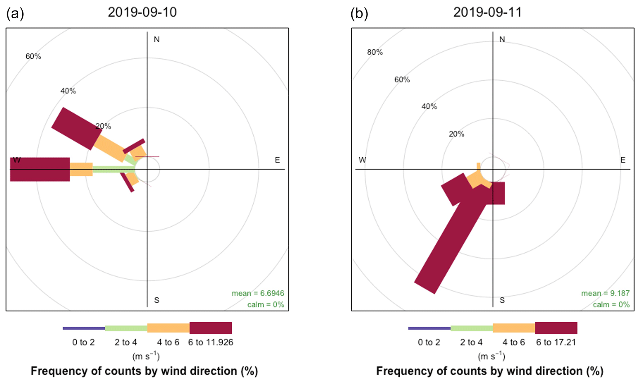
Figure 3 Wind rose with wind speed and direction for 10 September (a) and 11 September 2019 (b, Stern 3).

As the diffusive flux was calculated using the wind speed data, the CH₄-related parameters are also described separately for the two days. On 10 September, dissolved CH₄ concentrations showed a median of 22.6 nmol L⁻¹ (range 3.9–304.9 nmol L⁻¹). High CH₄ concentrations were encountered near Cuxhaven and at two to three patches between Helgoland and Cuxhaven (Fig. 4). On 11 September, concentrations were lower, with a median of 12.3 nmol L⁻¹ (range 1.1–175.8 nmol L⁻¹). The lowest concentrations (1–2 nmol L⁻¹) were encountered west of the islands of Scharhörn and Neuwerk.

Atmospheric CH₄ concentrations had a median of 1.949 ppm (range 1.936 to 1.971 ppm) on 10 September versus a median of 2.064 ppm on 11 September (range 1.948–2.255 ppm). On 11 September, rather high values (2.15 ppm) were observed near the island of Scharhörn. As the atmospheric CO₂ data were not elevated at this site, the influence of ship exhausts can be excluded. The wind came from south-southwest (200°), and the tide just increased. We assume that the air mass crossing our cruise track had an inherent natural variability.

The diffusive flux was first calculated with in situ wind and in situ atmospheric CH₄ concentrations (flux 1, flux 2 and flux 3 data are shown in Table 2 and described in Sect. 3.3). For both days combined, the average flux was 221 ± 351 µmol m⁻² d⁻¹, the median was 97 µmol m⁻² d⁻¹ and the range was from −27 to 2342 µmol m⁻² d⁻¹. On 10 September, the diffusive flux had a median of 131 µmol m⁻² d⁻¹ (range 316–1500 µmol m⁻² d⁻¹), with the lowest values near Helgoland and near the island of Scharhörn (Fig. 4, left). The highest values were observed southeast of Helgoland. On 11 September, the diffusive flux was half of that on the day before with a median of 62 µmol m⁻² d⁻¹ (range −27 to 2342 µmol m⁻² d⁻¹). The highest values were observed again in the region between Helgoland and Cuxhaven; the lowest and negative values were observed west of Cuxhaven (Fig. 4 right).

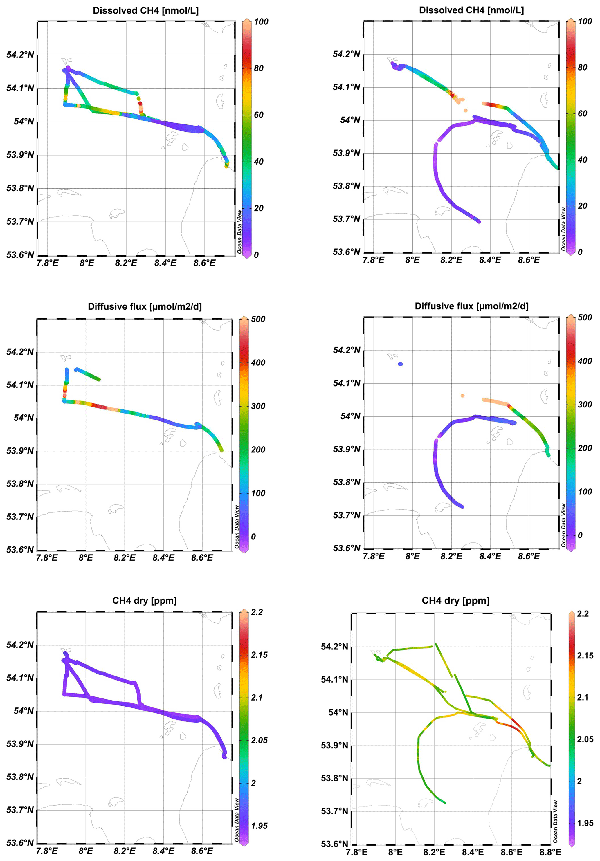
Figure 4 Concentrations of dissolved CH₄ (top), diffusive CH₄ flux (middle) and in situ atmospheric CH₄ concentrations (bottom) on 10 September (left) and 11 September (right). Schlitzer, Reiner, Ocean Data View, https://odv.awi.de, 2024.

3.2 Oceanographic and meteorological conditions in September 2020 (Stern 5)

Water temperatures in the study area in September 2020 were warmer compared to 2019, ranging from 17.6 to 21.4 °C, salinity ranged from 13.8 to 33.4 and oxygen saturation ranged from 70 % to 109 %.

The meteorological situation differed substantially between the sampling dates, and therefore the data are presented per day (and not for the whole area). On 31 August, the mean wind speed was 2.6 ± 2.2 m s⁻¹ coming from the north-northwest. On 1 September, the wind direction shifted towards northeast, with a mean speed of 4.5 ± 1.9 m s⁻¹. On 2 September, wind speed decreased to 2.3 ± 1.4 m s⁻¹ with no preferred direction. On 3 September, the wind speed increased to a mean of 7.6 ± 3.7 m s⁻¹ and blew from the south and south-southwest (Fig. 5).

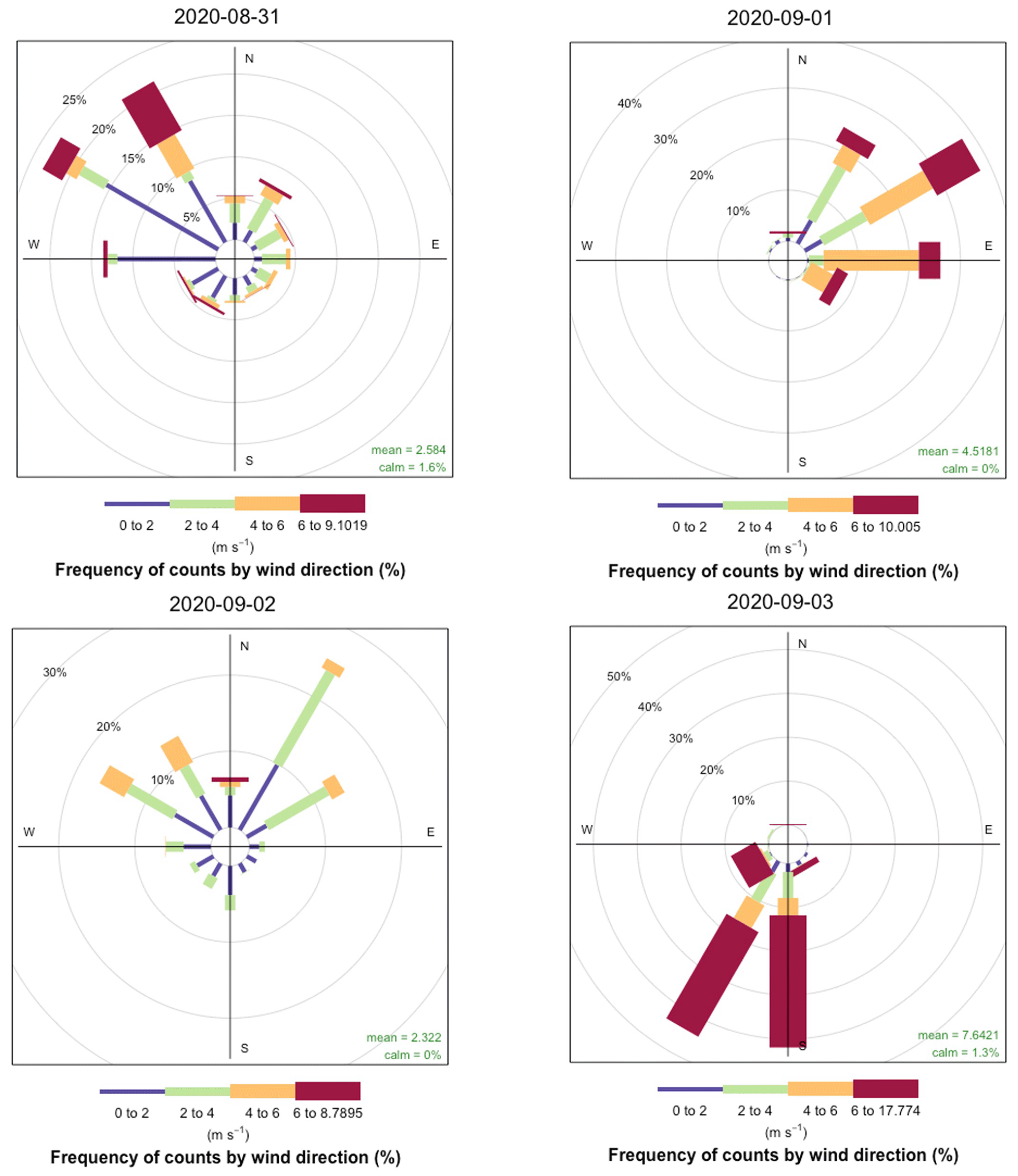
Figure 5 Wind rose with wind speed and direction for 31 August to 3 September 2020 (Stern 5).

Dissolved CH₄ concentrations for all days ranged from 1.4 to 607.9 nmol L⁻¹, with a median of 26.2 nmol L⁻¹ (Fig. 6, left). Low concentrations of dissolved CH₄ (5–10 nmol L⁻¹) were observed southwest of Helgoland, in the outer Weser Estuary and in the northern region of the study area towards the island of Sylt (Fig. 6, left). West of Büsum, we observed an area of high concentrations, as well as near Amrum, i.e., near the North Frisian Wadden Sea (> 100 nmol L⁻¹), with additional patches of elevated concentrations (70–100 nmol L⁻¹) located, for example, east and north of Helgoland.

The average diffusive CH₄ flux (flux 1) was 159 ± 444 µmol m⁻² d⁻¹ (flux 2 and flux 3 data are shown in Table 2 and described in Sect. 3.3). The median diffusive CH₄ flux for all days combined was 61 µmol m⁻² d⁻¹, ranging from 0.2–4645 µmol m⁻² d⁻¹. The spatial distribution of the flux was mostly a mirror image of the dissolved CH₄ concentration (Fig. 6, right). For the dataset from RV Littorina no flux data were calculated, as no wind data were available. The data for dissolved and atmospheric CH₄ and the diffusive CH₄ flux for the individual days are shown in Fig. S4, analogous to Fig. 4.

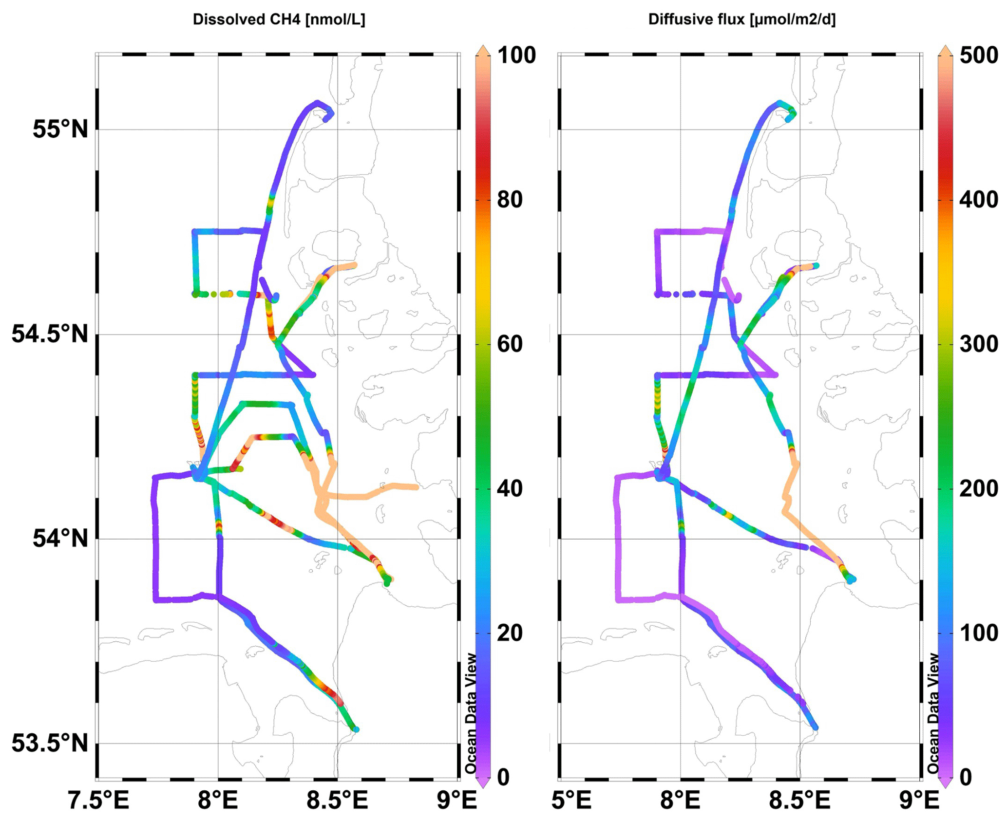
Figure 6 Concentrations of dissolved CH₄ (left) and the diffusive CH₄ flux (right) for the whole study area and study period of Stern 5 (31 August to 3 September 2020). Schlitzer, Reiner, Ocean Data View, https://odv.awi.de, 2024.

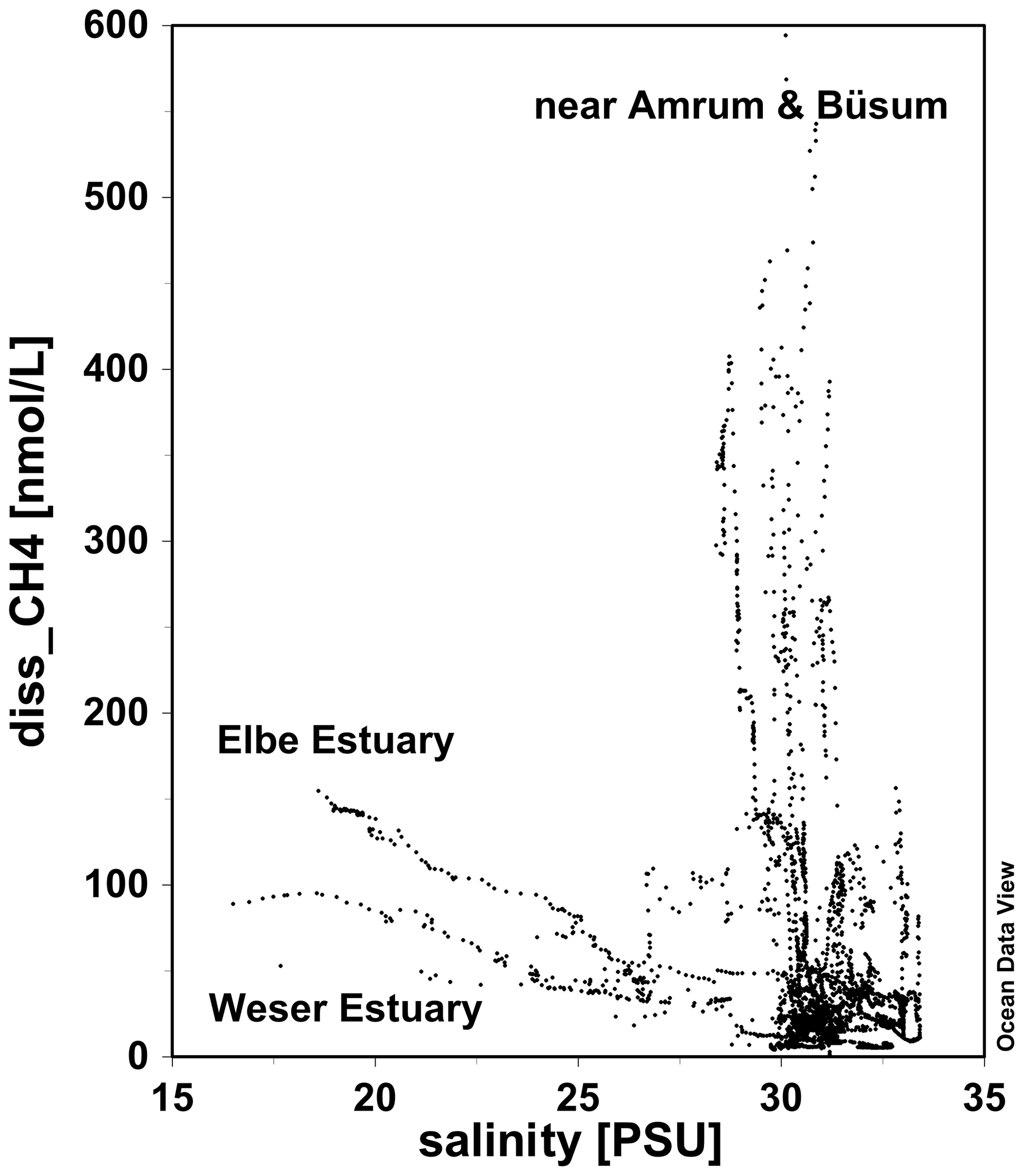
Figure 7 Dissolved CH₄ concentration plotted versus salinity for September 2020 (Stern 5). The geographic location of the data pairs is also indicated.

In both the Weser and Elbe estuaries, methane-rich river water was diluted with methane-poor marine waters (Fig. 7). The riverine endmember of the Weser showed lower CH₄ concentrations (95 nmol L⁻¹) than the Elbe endmember (151 nmol L⁻¹). However, the highest CH₄ concentrations coincided with high salinities (> 30). These concentrations were all observed in the area west of Amrum and Büsum in the Wadden Sea. Thus, these areas were clearly not part of the dilution scheme but a strong source of CH₄.

The median atmospheric CH₄ concentrations increased during the observed time span, from 1.951 ppm on 31 August, 1.979 ppm on 1 September and 2.022 ppm on 2 September to 2.078 ppm on 3 September (Fig. 8). This increase over time was especially evident when comparing 1 and 2 September. The same area was covered (as the ships returned to the same ports), and a substantial increase was observed, especially near the coast.

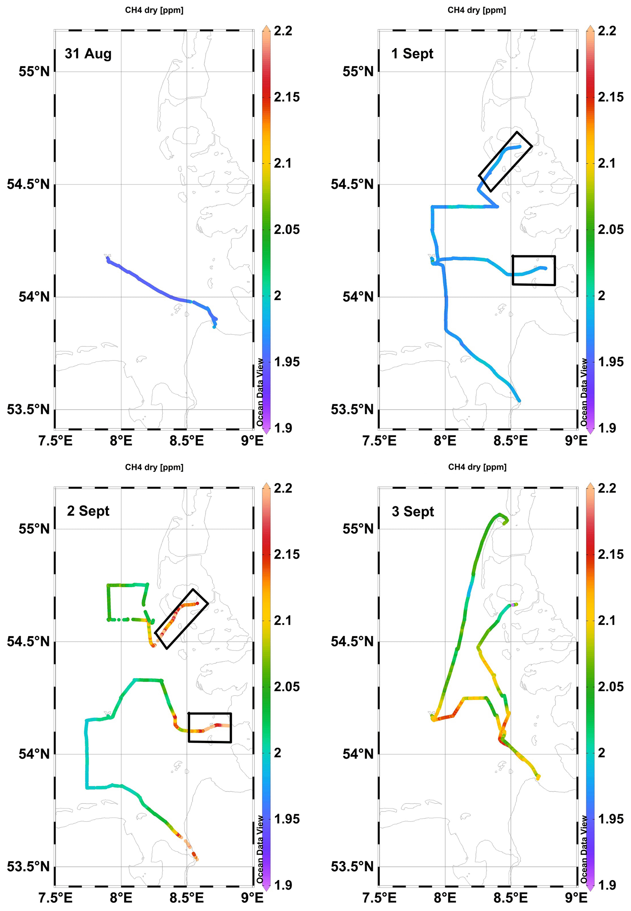
Figure 8 Atmospheric CH₄ concentration for 31 August to 3 September 2020 (Stern 5). The black boxes mark the areas where the vessels approached or left the Wadden Sea area. Schlitzer, Reiner, Ocean Data View, https://odv.awi.de, 2024.

3.3 Calculations of diffusive fluxes using in situ and land-station-based data

The calculation of the diffusive CH₄ flux was performed with three combinations of datasets to explore the influence that the use of atmospheric background data (for CH₄) and the closest land stations (for wind) has on CH₄ flux results (Table 1). For a better assignment of the wind data, the area was split into three boxes, one near Helgoland, one near Bremerhaven and one near Cuxhaven (see Figs. 1 and 2).

For the September 2019 cruises, the median in situ atmospheric CH₄ concentrations ranged from 1.950 to 2.060 ppm, compared to a monthly mean of 1.942 ppm at the Mace Head station (Table 2). For the wind speed, there was no or only a small difference between the in situ data and data from the weather stations in Bremerhaven and Helgoland, while for the Cuxhaven station wind speed was almost 4 m s⁻¹ lower than the in situ wind speed. Higher atmospheric CH₄ concentrations lead to higher equilibrium concentrations of dissolved CH₄ and therewith to a smaller oversaturation and lower diffusive fluxes. In 2019, the measured atmospheric CH₄ concentrations were always higher than those at the meteorological station. Consequently, the flux 2 values were often slightly higher than the flux 1 values (Fig. S5). The strongest difference was noticeable when comparing flux 1 with flux 3. When station data were used for both atmospheric CH₄ and wind (flux 3), there were substantial differences from the calculations using only in situ data (flux 1).

The median in situ atmospheric CH₄ concentrations ranged from 1.967 to 1.994 ppm for the September 2020 cruises, encompassing the monthly mean of 1.987 ppm at the Mace Head station (Table 2). The wind speed measured on board the vessels was always higher than the data from the stations, with a difference of 0.4 and 0.5 m s⁻¹ for Bremerhaven and Cuxhaven and a difference of 0.8 m s⁻¹ for Helgoland, resulting in comparatively lower flux 3 data. The flux 1 and flux 2 data were similar or almost identical, while flux 3 data were clearly different or lower than the other two fluxes (Fig. 9). For both years, the number of flux 3 data was higher than for flux 1 and flux 2. The wind data for flux 3 were taken from the meteorological station with hourly averages, while the in situ wind data were measured every minute but with data gaps due to the quality control of the data.

Table 2 The median concentrations of dissolved and atmospheric CH₄ and median wind speed in September 2019 and September 2020, calculated with in situ data, with monthly mean data from Mace Head station for atmospheric CH₄ or as hourly mean wind data from three weather stations at Bremerhaven, Cuxhaven and Helgoland. The calculation of the diffusive flux was performed according to Table 1. The flux calculations were performed for an area near Bremerhaven (area B), an area near Cuxhaven (area C) and an area near Helgoland (area H); see also Figs. 1 and 2.

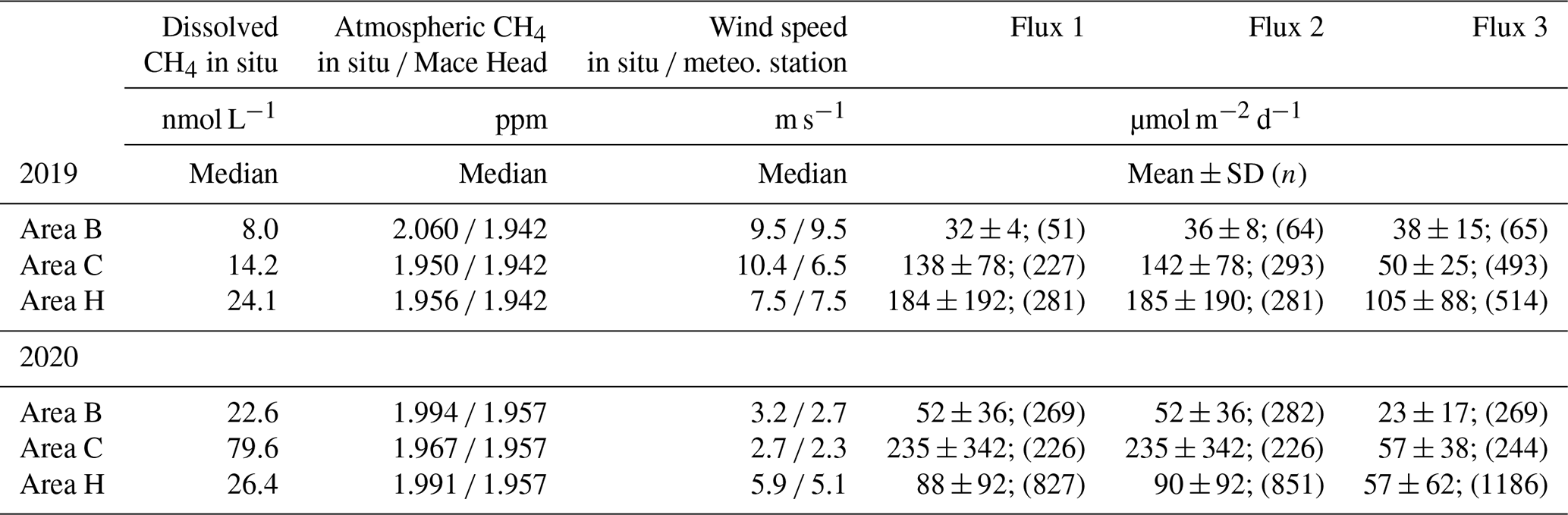
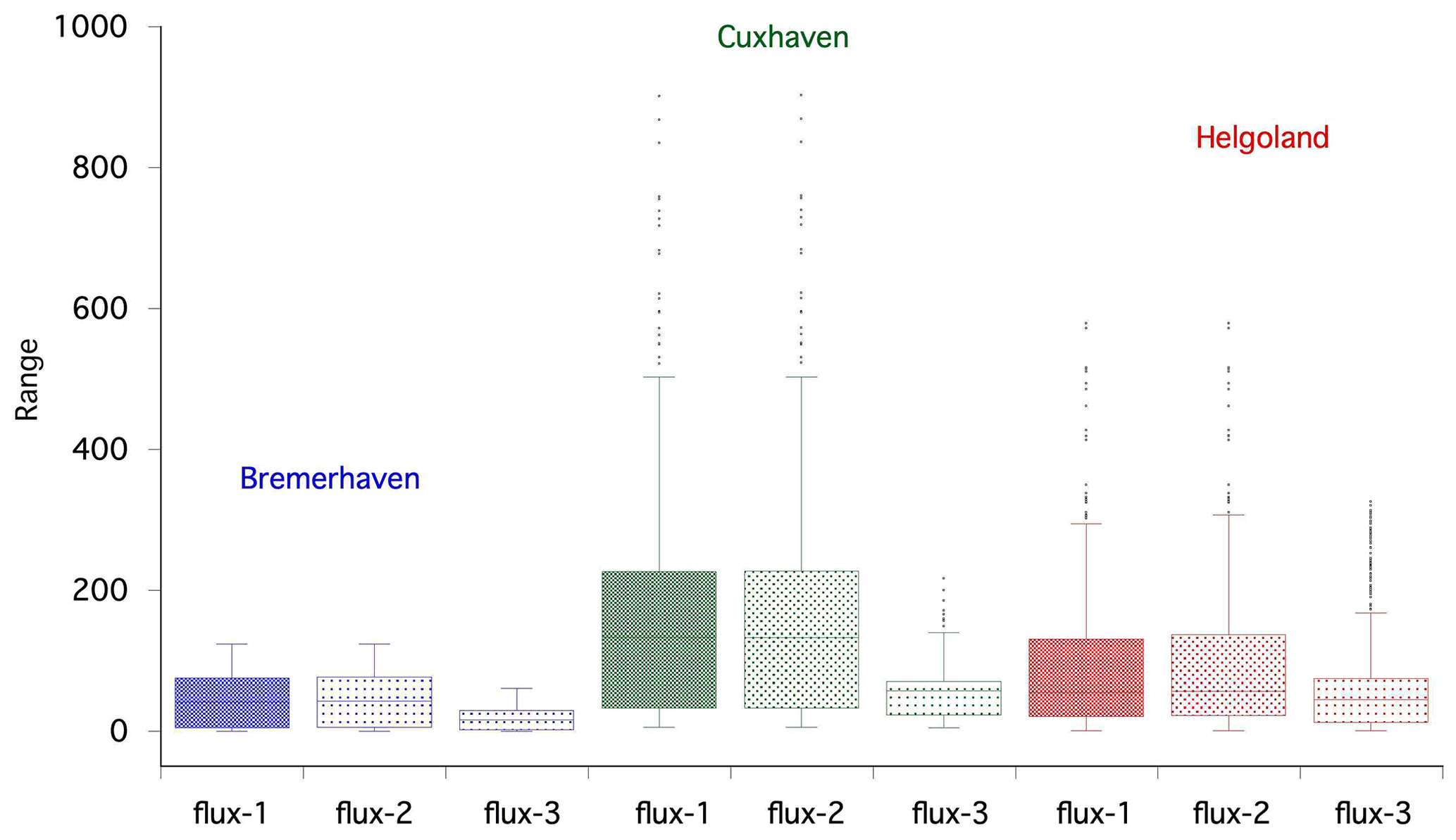
Figure 9 Range of diffusive CH₄ fluxes calculated with all in situ data from the cruises in September 2020 (flux 1), with in situ data and atmospheric CH₄ data from the land station (flux 2), and with in situ data and atmospheric CH₄ concentrations and wind from three land stations (flux 3). The calculations were performed for the regions of Bremerhaven (blue), Cuxhaven (green) and Helgoland (red); see Fig. 2.

3.4 Area-weighted calculation of the diffusive methane flux

The frequency distribution for the 2019 flux data is shown in Fig. S6. The majority of flux data (48 %) belonged to the range class 0–100 µmol m⁻² d⁻¹. The subsequent classes (100–500 µmol m⁻² d⁻¹) had frequencies of 40 % in total. Fluxes higher than 500 µmol m⁻² d⁻¹ had a total frequency of 9 %. Negative fluxes (−100 to 0 µmol m⁻² d⁻¹) occurred with a frequency of 3 %.

The frequency distribution for the 2020 flux data is shown in Fig. S7. Again, most of the data were found in the 0–100 µmol m⁻² d⁻¹ class, with a frequency of 67 %. The next class, 100–200, had a frequency of 21 %; the 200–300, 300–400 and 400–500 classes had a total frequency of 7 %. Fluxes higher than 500 µmol m⁻² d⁻¹ had a total frequency of 5 %. In contrast to the September 2019 values, negative fluxes (in the range of −100 to 0 µmol m⁻² d⁻¹) were not observed.

To calculate the weighted flux for our study area, we related the total area of Helgoland Bay (3.78×10⁹ m²) to the frequency of the flux classes, as explained in the “Material and methods” section and in supplementary Table S1. This resulted in the total area-weighted diffusive fluxes of 836 ± 32 and 600 ± 21 kmol d⁻¹ for the area of Helgoland Bay for 2019 and 2020, respectively.

The other approach was to multiply the median or mean of all flux data by the total area. The standard deviation for the mean was also multiplied by the area to maintain the same unit. This resulted in much lower values for the median flux data and identical values for the mean flux data compared to the area-weighted approach. However, the standard deviation of the mean flux data was much larger than for the area-weighted approach (Table 3).

Table 3 Comparison of three approaches used to calculate the total diffusive flux from Helgoland Bay with an area of 3.78×10⁹ m² based on the median, mean or area-weighted diffusive flux.

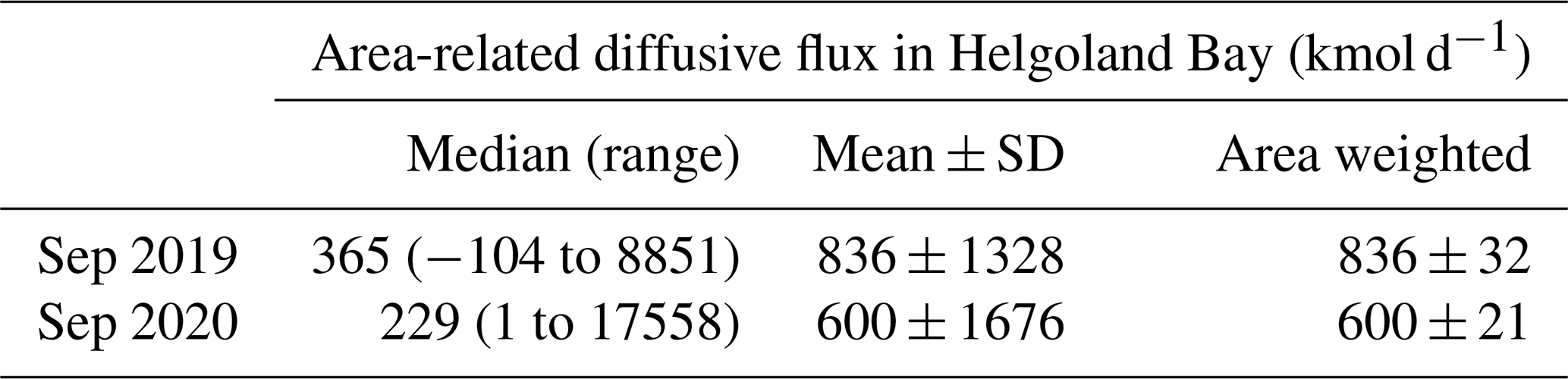
Table 4 Atmospheric CH₄ concentration in relation to tidal state, wind and diffusive CH₄ flux.

3.5 Estimation of flux contributions to atmospheric concentrations

We often observed a substantial increase in atmospheric CH₄ concentration between single days, but the source of the additional atmospheric CH₄ was unclear. Sources could be the diffusive flux from the sea into the atmosphere or different origins of the air masses above the water.

In September 2019, we observed an increase in atmospheric CH₄ concentrations of 0.116 ppm between 10 and 11 September (from 1.950 to 2.065 ppm). The average diffusive flux on these two days was 222 µmol m⁻² d⁻¹.

Using the ideal gas law, we converted the CH₄ flux into a gas volume (air temperature of 16 °C, pressure of 1015 mbar and time frame of 1 d, comparable to the calculations of Zang et al., 2020). Under the idealized assumption that we had no advective exchange, the diffusive flux alone would explain the observed concentration difference for a mixed atmospheric layer of 45 m in height.

In September 2020, the strongest difference in atmospheric CH₄ was observed between 1 and 2 September (delta = 0.079 ppm). The average diffusive flux for these 2 d was 48 µmol m⁻² d⁻¹. The calculation for the idealized mixed-layer height for this day yielded 15 m. Further assuming a planetary boundary layer height for mid-latitudes of about 300 m (a lower-range estimate based on climatologies by Ao et al., 2012) and a well-mixed surface layer of about 10 % thereof, i.e., 30 m, the observed increase in atmospheric CH₄ in September 2019 could have been mainly due to diffusive flux from the sea into the atmosphere. In September 2020, however, the calculated height of the mixed surface layer would be 15 m, which is not realistic. Thus, the observed increase in atmospheric CH₄ has to be attributed mainly to advection.

A linear regression analysis between the diffusive flux and atmospheric CH₄ revealed no significant correlation, also when split by single dates. Strong wind results in an increased diffusive flux, but as the mixing of the atmospheric CH₄ also increases, the signal of the diffusive CH₄ imported will be “diluted”. Thus, we tested the hypothesis that a correlation would be detectable only under low-wind conditions. Therefore, we split the wind into classes (< 10, < 9, < 8 m s⁻¹, etc.) and repeated the analyses for each class. These class-separated calculations revealed no correlation between the diffusive flux and atmospheric CH₄ concentration at wind speeds > 5 m s⁻¹. However, at wind speeds less than 5 m s⁻¹, a significant correlation between diffusive flux and atmospheric CH₄ was detected (r²=0.52). The strongest correlation was detected at wind speeds < 2 m s⁻¹ (r²=0.75).

A further possible cause for increases in atmospheric CH₄ concentrations is changes in advection under the assumption that wind coming across the sea has a lower CH₄ content than wind coming from land. As wind direction is not a linear parameter, we divided the parameter into 30° classes, followed by a one-way analysis of variance. The analysis revealed that the wind direction had a significant influence on the atmospheric CH₄ concentrations in our two study periods of September 2019 and September 2020 (p < 0.001).

In September 2019, the highest atmospheric CH₄ concentrations were observed when the wind came from south-southwest (210–240°), with a median of 2.08 ppm, and the lowest values were observed when the wind came from northerly directions (0–30, 300–330, 330–360°), with a median of 1.94, 1.95 and 1.95 ppm, respectively. In September 2020, the highest atmospheric CH₄ concentrations were observed when the wind came from the south (180–210°), with a median of 2.07 ppm, and the lowest values were observed when the wind came from the east (90–120°), with a median of 1.98 ppm.

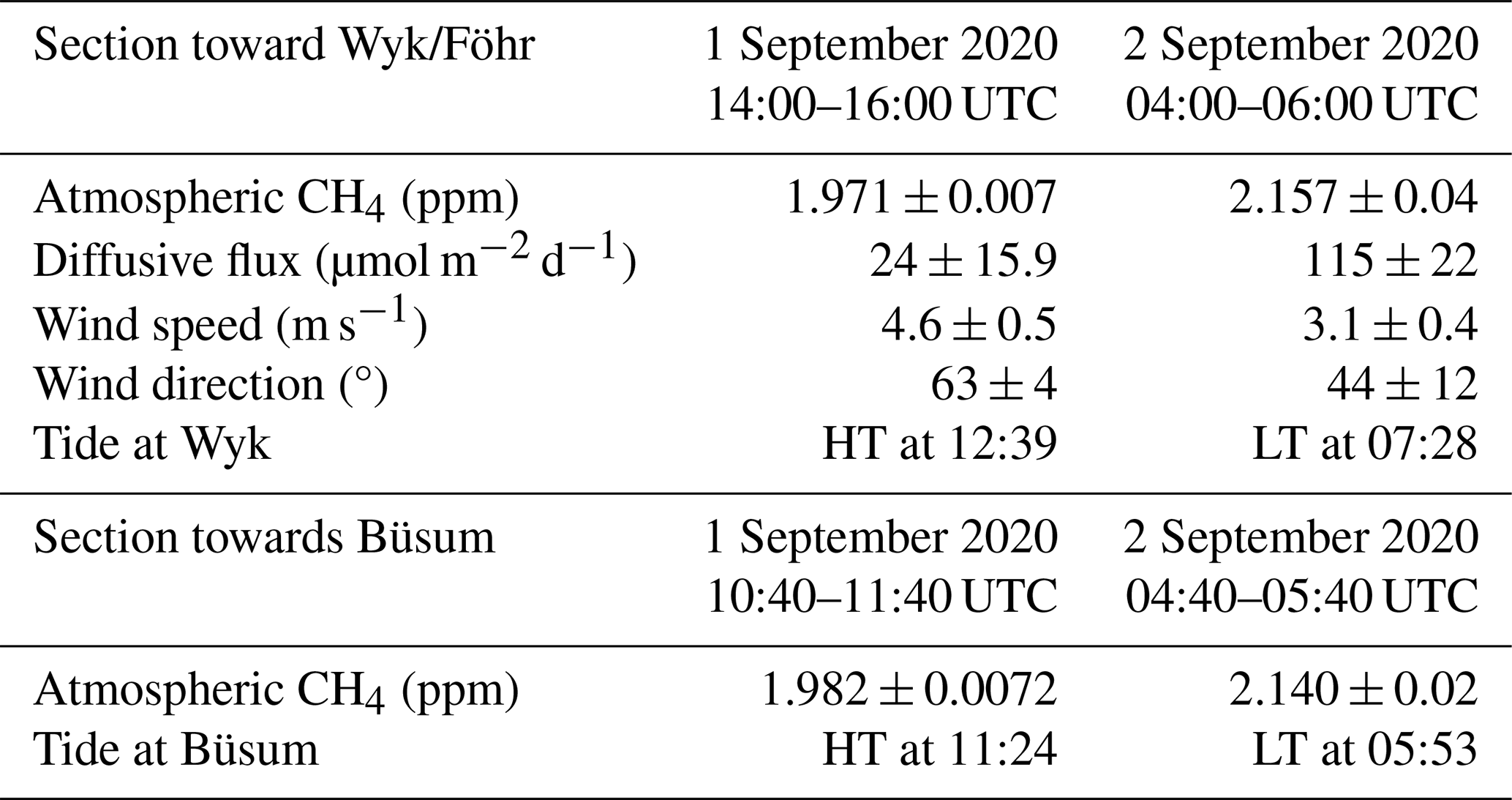
In addition to the wind signal, we looked for a possible tidal impact. On 1 September 2020, the RV Ludwig Prandtl approached the harbor at Wyk auf Föhr from 14:00–16:00 UTC and left the port around 04:00–06:00 UTC the following morning (Fig. 8). The wind blew from the northeast on both occasions, with a rather low wind speed of less than 5 m s⁻¹ (Fig. 5). High concentrations of dissolved CH₄ were observed as the harbor drew closer (the data points outside the dilution scheme of Fig. 7). The diffusive CH₄ flux increased, and a most pronounced increase of 0.186 ppm of atmospheric CH₄ was observed (Table 4). In contrast to the overall analyses described above, for this areal section neither wind speed nor diffusive flux was correlated with atmospheric CH₄. However, as Wyk auf Föhr is surrounded by the tidal flats of the Wadden Sea, at low tide these flats are exposed to the atmosphere, and tidal creeks withdraw porewater from the surroundings, which results in increased atmospheric CH₄ due to the release of CH₄ formed through anaerobic processes. A similar pattern of atmospheric CH₄ was observed for the tidal area off Büsum in the cruise section covered by RV Littorina. Atmospheric CH₄ increased for this section from 1.975 to 2.193 ppm; however no additional data (wind, diffusive CH₄ flux) are available for this ship.

4 Discussion

4.1 Error discussion for calculations of diffusive fluxes using different source data

The calculation of the diffusive sea–air flux depends highly on the parameterization of k. The most frequently used formula is the one from Wanninkhof (2014). For comparison we applied this formula to our dataset from 2020: the average flux was very similar 153 ± 441 µmol m⁻² d⁻¹ according to Wanninkhof versus 159 ± 444 µmol m⁻² d⁻¹ according to Nightingale. Both parameterizations should provide good estimates for most insoluble gases at intermediate wind speed ranges (3–15 m s⁻¹). Our wind data ranged from 1–11 m s⁻¹.

The study of Ho et al. (2018) concludes that if the mean depth of the water body is greater than 10 m, an ocean wind speed–gas exchange parameterization could be used in such environments. The mean water depth in our study area was 19 ± 12 m in 2019 and 17 ± 13 m in 2020. We therefore believe that the parameterization of Nightingale is appropriate for our study area. However, it should be kept in mind that this parameterization also holds an uncertainty of 19 %. Other factors influencing the parameterization of k are rain (which did not occur during our cruises), waterside convection and a biological surfactant suppression term (Gutiérrez-Loza et al., 2021). During summer, convection and surfactants seemed to act as competing mechanisms controlling the flux. Convective processes enhanced the downward flux slightly, while surfactants tended to suppress it (Gutiérrez-Loza et al., 2021).

In this study we applied several different methods to calculate diffusive sea-to-air CH₄ fluxes, either by using different databases for local values or by applying a weighted method for CH₄ fluxes for larger areas.

The comparison between results obtained using different data sources showed that the choice between using atmospheric CH₄ concentrations from in situ data or from a land station did not have a large effect (flux 1 versus flux 2, Fig. 9). In our study, the monthly average atmospheric CH₄ concentration from Mace Head station, which is usually used for providing atmospheric background concentrations, always showed lower values than our in situ data. Thus, the saturation concentration of dissolved CH₄ was lower, resulting in a smaller sea-to-air diffusive flux. However, in relation to the variability of the measured datasets, this difference was minor. The calculated flux 2 values reached on average 103 ± 6 % of the corresponding flux 1 values (n = 6).

In contrast, it was important to use the in situ wind speed for calculating the CH₄ fluxes (flux 3) instead of using data from the closest meteorological land stations. In some cases, the wind data were nearly identical; in other cases the wind data from the land monitoring stations were lower, resulting in significantly smaller diffusive fluxes. The stronger impact of the wind speed is based on the fact that the flux calculation uses a quadratic wind speed formulation (Eq. 2, Nightingale et al., 2000). Relating the flux 3 (land station) data to the flux 1 (in situ) data revealed that the flux 3 values only reached an average of 58 % ± 34 % of the flux 1 values (n = 6). As our flux data have a high variability (see below), a high temporal resolution of the data (as in flux 1) is favorable over hourly (wind data) or monthly (atmospheric CH₄ data) resolution. Several combinations of in situ data and data from databases have been reported in the literature for calculating diffusive sea-to-air CH₄ fluxes (Myllykangas et al., 2020; Woszczyk and Schubert, 2021; Mau et al., 2015; Bussmann et al., 2021b; Humborg et al., 2019). Based on our direct comparison of these different approaches, we strongly recommend obtaining in situ wind data.

We furthermore observed a high variability in all diffusive CH₄ flux data. For the entire 2019 dataset, the average diffuse CH₄ flux was 221 ± 351 µmol m⁻² d⁻¹ (n = 941), and for 2020 it was 159 ± 444 µmol m⁻² d⁻¹ (n = 3028). The coefficient of variation (CV) was 158 % and 279 %, respectively. Flux values for CH₄ in general have a high variability (36 %–71 %, de Groot et al., 2023; 73 %, Bussmann et al., 2021b; 78 %, Humborg et al., 2019); thus, the CV values found here are not unusual. However, to avoid a possible elevated flux variability due to a small sample size (methodological error), we applied a modified bootstrap analysis on the 2020 data to elucidate the effect of sample size on the calculated flux variability. The 2020 dataset had a total of 3028 measurements. From this dataset, we iteratively drew random subsamples, beginning with 20 values and increasing the sample size by 10 and 100 in each iteration. With this method, we finally had 39 datasets with an increasing number of flux values, starting at 20 and reaching up to 3028 values. The mean of these 39 datasets was calculated and plotted versus sample size (Fig. 10). The analysis revealed that the calculated average mean flux was independent of the sample size (slope, t=0.02, p=0.98) and that the variability of the flux values remained stable between 104 and 190 µmol m⁻² d⁻¹, with an average mean value of approximately 156 µmol m⁻² d⁻¹ for a sample size of about 900–1000 or higher. This supported our presumption that our sample size of 3028 for the year 2020 was sufficiently high to avoid a sample size bias in flux variability and represented a realistic system flux in the area. This high spatial variability is also evident in Fig. 6. Thus, it is debatable if our study area is a uniform area and if it is reasonable to average the diffusive flux for the whole study area.

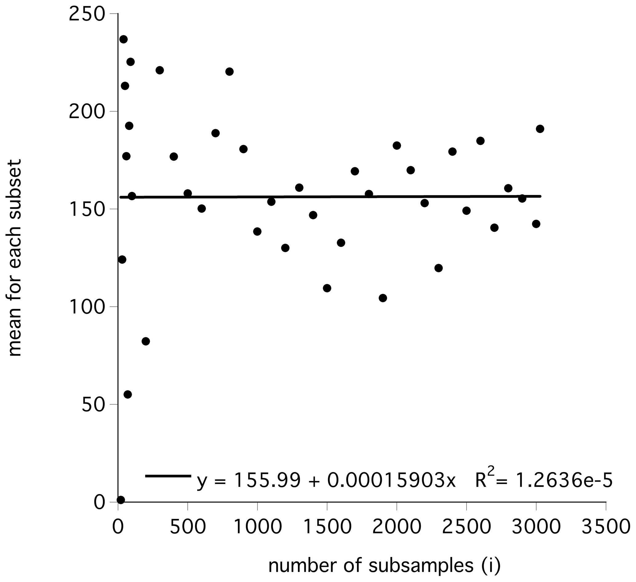
Figure 10 The mean of the diffusive CH₄ flux calculated for a random number of i subsamples. The black line indicates the regression line.

4.2 Area-weighted calculation of the diffusive CH₄ flux

To extrapolate the diffusive flux for larger areas (in mol d⁻¹), the general approach is to multiply the target area (m²) by the median or mean flux (mol d⁻¹ m⁻²) calculated from a restricted number of samples in the area. Figures S4 and S5 show the database and frequency distribution for such a calculation for our data between the years 2019 and 2020. Both figures show a highly skewed distribution of flux values, with values < 100 µmol m⁻² d⁻¹ having the largest share, resulting in a skewness of 3.4 and 6.1 for 2019 and 2020, respectively. Table 3 shows the results of different methods of averaging when calculating the diffusive flux for our target areas in 2019 and 2020.

According to common recommendations for data with a positive skew (data with the frequency distribution shifted to the left side), the median is always smaller than the mean (median < mean) (Köhler et al., 1996; Doane and Seward, 2011). Accordingly, the median in our calculations revealed almost 3-fold lower overall flux estimates compared to the mean values. To circumvent this bias, a variety of terrestrial, marine and limnic studies (Mallast et al., 2020; Li et al., 2020; Baliña et al., 2023) have stressed the importance of applying an area-weighted approach to upscale CO₂ flux data. We therefore also applied this method to our data (Table 3, right column). This calculation revealed that flux values for the area calculated by using the arithmetic mean are identical to the area-weighted mean values and significantly higher than the median-based average flux values. In addition, the SD from the area-weighted flux was much lower. Thus, if area-weighted flux estimations are not possible due to a limited dataset, our data suggest that using the mean value rather than the median-based average flux calculations for an area is the preferred procedure.

4.3 Methane emissions from Helgoland Bay

In our study we revealed mean diffusive fluxes of 221 ± 351 and 159 ± 444 µmol m⁻² d⁻¹ and median values of 97 and 61 µmol m⁻² d⁻¹ for 2019 and 2020, respectively.

These numbers are within the same range as those published previously for June 2019 (65 µmol m⁻² d⁻¹) (Bussmann et al., 2021b). However, higher flux data are reported for autumn and winter: 104 µmol m⁻² d⁻¹ for the Dogger bank area (Mau et al., 2015) and 124–299 µmol m⁻² d⁻¹ for our study area (Winkler, 2019) (all median values). These higher fluxes were explained by the authors with higher wind velocities in the autumn/winter season. In comparison to other coastal seas, our diffusive fluxes are similar to fluxes from the Belgian North Sea (161–221 µmol m⁻² d⁻¹ (Borges et al., 2019). In contrast, much higher fluxes are reported from the Baltic Sea, with −9 to 3110 µmol m⁻² d⁻¹ by Gutiérrez-Loza et al. (2019) and 2400 µmol m⁻² d⁻1 by Humborg et al. (2019). On the other side, low fluxes are reported from the Atlantic coast of Spain (7–20 µmol m⁻² d⁻¹; Ortega et al., 2023) and coastal Chile (5 ± 5 µmol m⁻² d⁻¹; Farías et al., 2021).

However, these comparisons are all based on the median values for the whole area. When focusing on specific locations, other patterns become evident. The lowest fluxes, i.e., negative fluxes, were observed in September 2019 in an area west of Cuxhaven (−15 to −27 µmol m⁻² d⁻¹, Fig. 4b). At this site and at this time, the water was shallow (< 5 m), with strong winds from southwest resulting in short waves. Thus, we assume that this water body was mostly depleted of CH₄ and acted as a CH₄ sink. For the open North Sea, other studies have reported undersaturation of dissolved CH₄ (Upstill-Goddard et al., 2000) (Bange, 2006) but not for nearshore areas like in this study.

The highest CH₄ concentrations were observed in the Wadden Sea and were not related to river water inputs (Fig. 7). Elevated diffusive fluxes and elevated atmospheric concentrations were also observed at these locations, especially at low tide (Table 4). Sand flats or tidal flats are known to be a source of biogenic CH₄ that is released directly into the water column of the North Sea and into the atmosphere during low tide (Wu et al., 2015; Beck and Brumsack, 2012). It has been reported that peaks in CH₄ coincided with ebb tides at multiple sites located along the flanks of the estuary adjacent to tidal flats and wetlands (Pfeiffer-Herbert et al., 2019; Trifunovic et al., 2020). Another aspect of elevated CH₄ concentrations is the distance to the coast, as described in several studies (Sierra et al., 2020; Thomas and Borges, 2012). However, no such correlation was observed in this study, probably due to the highly diverse coast (Wadden Sea, sandy beaches, estuaries) superimposed by tidal cycles.

4.4 Estimation of sea–air flux contribution to atmospheric concentrations

The average atmospheric CH₄ concentrations in this study were 2.03 ± 0.08 and 2.05 ± 0.08 ppm for September 2019 and 2020, respectively. This is about 0.06 ppm higher than the values from Mace Head at the west coast of Ireland. Since 2020, two new Integrated Carbon Observation System (ICOS) stations have been installed on Helgoland and Sylt, which are located in or near our study area. Their average September data (2021 and 2022) of 2.04 ± 0.07 and 2.04 ± 0.08 ppm support our elevated atmospheric CH₄ concentrations (Kubistin et al., 2023; Couret and Schmidt, 2023).

One aim of our study was to clarify if, or under which circumstances, the diffusive flux from the water is detectable in the atmosphere above. An increased wind speed will lead to an increased CH₄ flux into the atmosphere above the water; however, this process is counteracted by the fact that increasing wind speed also leads to increased mixing of the atmosphere, and any input will be quickly diluted.

Our study has shown that there is only a significant correlation between CH₄ fluxes and atmospheric CH₄ concentrations at wind speeds < 5 m s⁻¹. For example, when we observed a strong increase in atmospheric CH₄, we estimated whether this increase was due to CH₄ input from the sea. For September 2019, the increase in atmospheric CH₄ could be attributed to the input from the sea but not for September 2020. Thus, the static approach of Zang et al. (2020) could not be confirmed by our data, as this approach does not take the turbulent mixing of the atmosphere into account. Several other studies, which also measured atmospheric CH₄ concentrations and diffusive fluxes simultaneously, confirm this absent relationship (Myhre et al., 2016; de Groot et al., 2023; Gutiérrez-Loza et al., 2019). From our more detailed estimates, we conclude that the comparison of diffusive fluxes and atmospheric concentrations alone does not account for the interactions of diffusive flux and atmospheric convection. More insights could be obtained from inverse atmospheric modeling or model-based extrapolation approaches (Saunois et al., 2020; Bittig et al., 2024), but these are beyond the scope of this study. In future studies with further cooperation, our dataset might be used for these approaches.

Wind direction and advection of air masses have a strong influence on atmospheric CH₄ concentrations (Pankratova et al., 2022; Yang et al., 2019). Our data show that when the wind came from the south or south-southwest, significantly higher atmospheric CH₄ concentrations were observed (2.07–2.08 ppm). Wind from this direction originated from the German mainland from the ports of Bremerhaven and Wilhelmshaven and from regions with intensive livestock farming. Our air mass origin assumptions are supported by results from the NOAA back-trajectory modeling (at 10 m height, https://www.ready.noaa.gov/hypub-bin/trajasrc.pl, last access: 12 October 2023). Air masses at the end of 3 September 2020 originated from the mainland of Lower Saxony and the Netherlands (Fig. S8). On the other hand, the lowest atmospheric CH₄ values were observed when the wind blew from the north (1.95 ppm) in 2019. Wind from this direction originates from the open North Sea and shows similar values to those observed at the NOAA Mace Head station in Ireland (1.965 ppm). However, in 2020, easterly winds advected low atmospheric CH₄ concentrations (1.98 ppm). These winds originated from the less populated and more agriculturally used land areas of Schleswig-Holstein or even from the Baltic Sea. The mean wind speed of these easterly winds was 5 m s⁻¹, and the distance from Helgoland to the Baltic is about 200 km. Thus, the wind covered this distance within 11 h, and the air masses we measured could have come from an open sea area again, this time the Baltic Sea. This air mass origin is supported by the NOAA modeling, as air masses observed in our study area at the end of 1 September 2020 originated from Schleswig-Holstein and the Baltic Sea (Fig. S8).

5 Conclusions

In our study we compared different methods to calculate the diffusive CH₄ fluxes with in situ data and data from land-based meteorological stations. The usage of in situ wind data (at high temporal resolution) was the most important, while the usage of in situ atmospheric concentration data showed no large difference from fluxes obtained using in situ data. When extrapolating from the measured data and from the real study area to a larger area (i.e., Helgoland Bay), it was important to use the arithmetic average and not the median value. Most natural data are skewed towards lower values, and using the median of these datasets would result in an underestimation of diffusive CH₄ flux. However, the area-weighted extrapolation is recommended, as it yielded the most realistic results with the smallest variability.

We observed large variability in our datasets, which was not due to methodological constraints but reflects the high natural variability of the study area. Thus, it is debatable if it is reasonable to average over a heterogeneous area such as Helgoland Bay. An improvement in flux estimates could be achieved by covering the whole area with a systematic zigzag track. New statistical methods are now available to overcome spatial and temporal restrictions of observed datasets, mostly for CO₂ (Bittig et al., 2024), and their application might give new insights.

Hot spots of CH₄ emissions were the tidal flats at low tide. Their CH₄ emissions resulted in locally elevated atmospheric CH₄ concentrations. However, in shallow water and rough sea, the coastal North Sea was undersaturated with CH₄ and acted as a CH₄ sink. Overall, the diffusive CH₄ flux into the atmosphere accounted for increased atmospheric CH₄ concentrations only at low wind speeds. Atmospheric advection was the main driver of low CH₄ concentrations (when coming from the sea) and high CH₄ concentrations (when coming from the mainland).

With our comprehensive study we revealed a complex relationship between dissolved CH₄ concentrations, CH₄ fluxes into the atmosphere and atmospheric CH₄ concentrations in shallow coastal water areas.