Anthropogenic carbon storage and its decadal changes in the Atlantic between 1990–2020

The Atlantic inventory of anthropogenic carbon (C_ant) and its changes between 1990 and 2020 are investigated by applying the transit time distribution (TTD) method to anthropogenic tracer data. In contrast to previous TTD applications, here we take into account the admixture of old waters free of anthropogenic tracers. The greatest difference from other methods based on direct carbon observations is the higher C_ant storage in the deep ocean. Estimations of the decadal C_ant increase based on direct carbon observations yield in general a smaller share of C_ant storage in the North Atlantic and a larger share in the South Atlantic compared to our results. Changes in oceanic circulation and/or ventilation have significant impacts on the C_ant inventory on the regional scale. The enhanced upwelling of older water in the Southern Ocean and the variability in the convection depth in the Labrador Sea lead to deviations in the inferred C_ant increase between 1990 and 2020 from the rate equivalent to a steady-state ocean. For the total Atlantic C_ant inventory, however, decadal ventilation variability of individual water masses partially compensates for each other. In addition, its impact on the C_ant storage is small due to the much higher flushing time for the whole Atlantic of the order of hundreds of years. The total C_ant inventory increases from 43.0 ± 7.3 Pg C in 1990 to 68.2 ± 10.8  Pg C in 2020, almost in unison with the rising CO₂ in the atmosphere. So far, ventilation changes have impacted the C_ant concentrations only on the regional scale, especially in the subpolar North Atlantic and the Southern Ocean.

1 Introduction

The ocean is an important sink for anthropogenic carbon (C_ant) emissions from, e.g., fossil fuel burning, cement production and land use change (Friedlingstein et al., 2020). Over the industrial era, about 30 % of these emissions have been taken up by the ocean (Gruber et al., 2019) (inferred from observations). Based on global biogeochemical models that meet observational constraints, Friedlingstein et al. (2020) find a slightly smaller ocean carbon uptake of about 25 % of the emissions over the last few decades. A decrease (< 5 % over the last few decades) in the fraction of the CO₂ emissions taken up by the ocean is to be expected due to the decreasing buffer capacity of the oceanic waters. In addition, a slower oceanic circulation and mixing in a warming climate might reduce the uptake rate of surface waters for human-produced carbon (Heinze et al., 2015). Future changes in the oceanic circulation may also alter the biological carbon pump and the storage of remineralized carbon (Heinze et al., 2015).

The North Atlantic is the region with the highest column inventory of anthropogenic carbon (or the highest storage rates over the industrial era), both in models and in observations (Sabine et al., 2004; Khatiwala et al., 2013). It is also a region with large variability in water mass formation, especially for Labrador Sea Water (Kieke et al., 2006; Rhein et al., 2007; Yashayaev, 2007; Kieke and Yashayaev, 2015; Yashayaev and Loder, 2016). These changes in water mass formation/ventilation also have an impact on the inventories of C_ant (Steinfeldt et al., 2009; Pérez et al., 2013; Rhein et al., 2017), with relatively small C_ant storage rates for periods with less intense convection, such as the 2000s (Raimondi et al., 2021; Müller et al., 2023). Our study also addresses these impacts. In particular, it comprises the time frame with deep and intense formation of Labrador Sea Water (1987–1995); the following period of weaker convection (1996–2013) (Kieke et al., 2007; Yashayaev, 2007; Kieke and Yashayaev, 2015); and the recent reinvocation of deep-reaching convection since 2014, accompanied by an increase in C_ant uptake and oxygen concentrations (Rhein et al., 2017).

C_ant in the ocean cannot be measured directly but has to be inferred by indirect techniques. One group of methods to calculate C_ant concentrations is the so-called “back-calculation techniques” (e.g., ΔC^∗, Gruber et al., 1996; $\mathit{\phi }{\mathrm{C}}_T^{\mathrm{0}}$, Vázquez-Rodríguez et al., 2009). These techniques rely on measurements of dissolved inorganic carbon (DIC), the assumed natural background concentration of DIC, and the DIC originating from both the remineralization of organic matter and the dissolution of calcium carbonate. Another technique is the extended multiple linear regression (eMLR) (Friis et al., 2005). Here, observations at two different times of both DIC and auxiliary quantities, such as temperature, salinity, nutrients and oxygen, are needed, which allow us to build a regression for DIC based on the other variables. Using this method, the difference in C_ant between the two dates can be determined but not the absolute value. Recently, Clement and Gruber (2018) developed an eMLR for C^∗, i.e., the observed DIC excluding the carbon from remineralization of organic matter and dissolution of calcium carbonate. This eMLR(C^∗) method has also been applied by Gruber et al. (2019) and Müller et al. (2023) to the observational data from the GLODAPv2 data set (Lauvset et al., 2024).

Other methods do not rely on directly measured carbon data. Instead, they take advantage of anthropogenic tracers like CFCs and SF₆ and lead to C_ant distributions that are more compatible with these tracers. These methods are the transit time distribution (TTD) method (Hall et al., 2002; Waugh et al., 2006) and the Green function (GF) approach (Holzer and Hall, 2000; Khatiwala et al., 2013). They consider C_ant to be a passive tracer that is advected from the surface into the ocean interior. Thus, these methods do not require making assumptions about the biochemical involvement of carbon (the biological pump) as is necessary for the aforementioned methods. On the other hand, they need to make assumptions about the temporal evolution of C_ant in the mixed layer of the ocean and the shape of the TTD or Green’s function. The TTD technique allows us to predict the C_ant concentrations from older observations – under the assumption that the ocean is in steady state. In this way, it is possible to distinguish whether C_ant changes between two time periods that (i) originate from the atmospheric CO₂ increase or (ii) are caused by changes in the ocean circulation.

The different C_ant calculation methods generally lead to inventory differences of the order of ± 10 %, both on the global scale (Khatiwala et al., 2013) and along basinwide sections in the Atlantic (Vázquez-Rodríguez et al., 2009). However, the vertical distribution of the inventory is different, with the ΔC^∗ method attributing a smaller fraction to the deep water masses (Vázquez-Rodríguez et al., 2009). This also holds true for recently ventilated deep and bottom waters. On the regional scale, the inventory differences are larger, especially in the Southern Ocean (Vázquez-Rodríguez et al., 2009). For the biogeochemical consequences of oceanic C_ant storage, such as ocean acidification, not only is the total oceanic C_ant uptake of importance, but also its local storage rates and the vertical distribution.

Here, we use a modified version of the TTD method to infer the inventories of C_ant over the Atlantic from 70° S to 65° N for the years 1990, 2000, 2010 and 2020. The method is mainly based on Steinfeldt et al. (2009) but additionally allows for the admixture of old waters free of anthropogenic tracers. The impact of this modification of the TTD method on the derived C_ant concentrations is described. We then quantify the decadal C_ant inventories and their changes and compare them with a steady-state ocean, where C_ant solely changes due to the rising atmospheric CO₂ concentration. This allows us to quantify the impact of changes in ocean ventilation and circulation on C_ant, i.e., the main processes storing C_ant in the ocean interior. We further discuss our results with respect to currently existing global studies and highlight and discuss prominent similarities and discrepancies.

2 Data and methods

2.1 Data and calculation of C_ant distributions

We use anthropogenic tracers (CFC-12, CFC-11, CFC-113, tritium and SF₆) to calculate transit time distributions (TTDs), from which the concentration of C_ant is finally inferred. The data are mainly taken from the GLODAPv2.2023 data product released in 2023 (Lauvset et al., 2024). The transient tracer data discussed here cover the period between 1982 and 2021. The GEOTRACES GA02 section from 2010/2011 (Schlitzer et al., 2018) and data from North Atlantic cruises conducted over the period of 2017–2018 and not contained in this data product have also been added here (Table 1). The salinity and transient tracer data of these additional cruises have underwent similar bias control procedures to those in the GLODAPv2.2023 data product, and no offset could be detected.

(Steinfeldt et al., 2023a)(Steinfeldt et al., 2023b)

Table 1 List of cruises used with transient tracer data not included in GLODAPv2.2023.

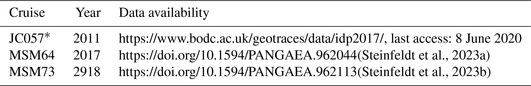
^* Part of GEOTRACES section GA02.

Table 2 Number of anthropogenic tracer samples used for the C_ant calculation.

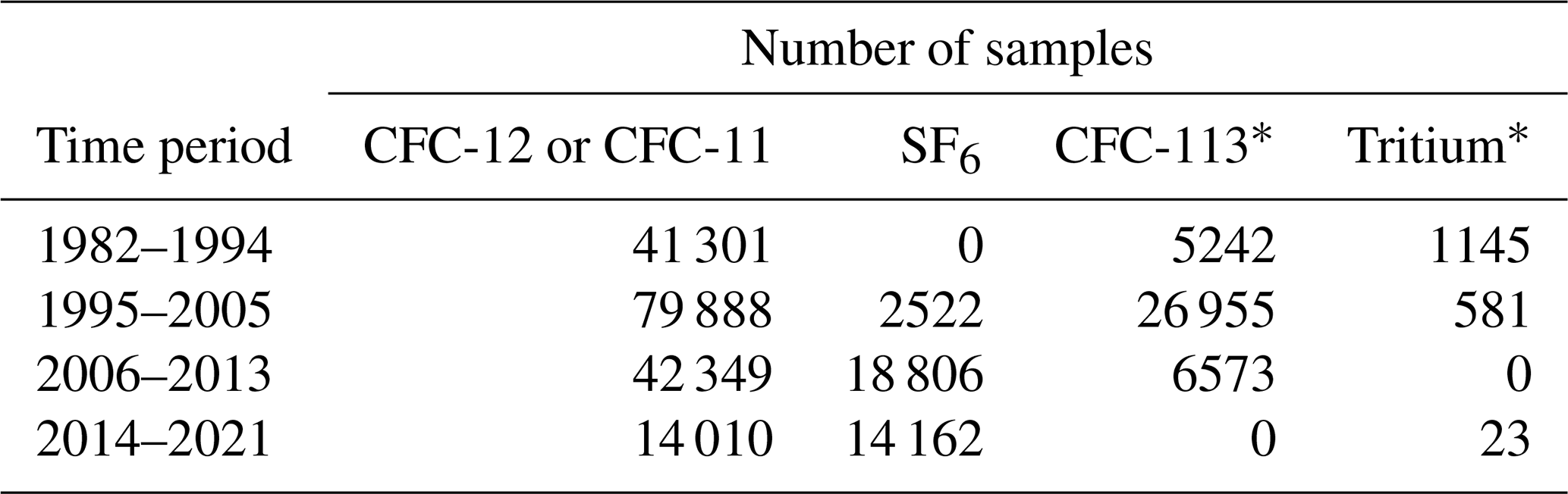
^* CFC-113 and tritium are only used to calculate the ratio of Δ to the mean age Γ of the TTDs independently of time; see Sect. 2.3.1.

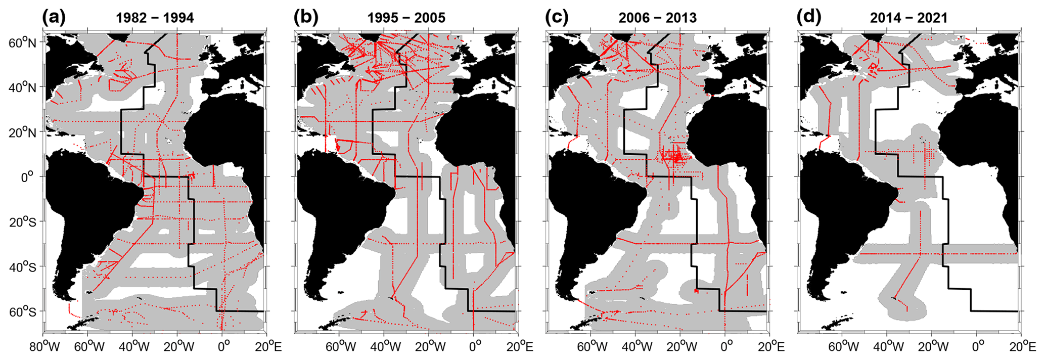
Figure 1 Location of ship stations with CFC-12 and/or CFC-11 data used for the C_ant calculation for the 4 decades considered here. (a) 1982–1994, (b) 1995–2005, (c) 2006–2013, (d) 2014–2021. The grey-shaded area indicates the region for which gridded C_ant data could be generated for the respective period. The thick black line following the Mid-Atlantic Ridge is used for separating the Atlantic Ocean into a western and eastern basin.

The data are grouped into four periods roughly centered around 1990, 2000, 2010 and 2020. These time segments include the years 1982–1994, 1995–2005, 2006–2013 and 2014–2021 respectively. The periods are chosen to allow for a good data coverage of the Atlantic at least for the first three periods. For the 2014–2021 time frame, the data are sparse except for the North Atlantic. The main focus of the last period is to investigate the effect of the reinvocation of deep convection in the Labrador Sea (Yashayaev and Loder, 2016) on the C_ant distribution. Table 2 shows the number of available tracer data for the four periods. The location of all profiles with CFC-12 and/or CFC-11 data for every decade is indicated in Fig. 1a–d. Tritium, CFC-113 and SF₆ are colocated with CFC-11 and/or CFC-12 but have much fewer data points. They are mainly used to infer the shape of the TTD (see Sect. 2.3.1) for the whole time period.

For the isopycnal interpolation of salinity, potential temperature and anthropogenic carbon, at each profile mean values of 38 density layers are calculated. The boundaries of these density intervals are given in Table A1. For the upper layers (σ_θ), the potential density referenced to the surface is used, for the intermediate layers (σ_1.5) 1500 dbar is used, and for the deep layers (σ₄) 4000 dbar is used. At some locations, the deepest σ_θ layer is located below the upper σ_1.5 layers. In this case, these upper σ_1.5 layers remain empty. The same holds true for the transition between σ_1.5 and σ₄. A mean value for a density layer is only calculated if at least one data point is located within that density interval. Typically, the number of density levels for a deep-reaching profile is about 30. The layers with the lightest densities only exist at low latitudes, and the densest σ₄ layers only exist in the Antarctic Bottom Water (AABW) core and in the North Atlantic south of the Denmark Strait.

The isopycnal mean values are then mapped horizontally (i.e., isopycnally) on a regular grid (0.25° latitude ×0.5° longitude) from 70° S to 65° N and 80° W to 20° E. As the number of available samples from the water bottles is typically around 20 per profile, some density layers might not get assigned a mean value. As these “empty” layers change from profile to profile, there are still enough points for each density layer to perform the gridding procedure.

The gridding method is similar to that applied in Rhein et al. (2015); i.e., an objective mapping scheme is used, where the weighting factor decreases with distance r from the data points (exp (−r²)). An additional weighting factor proportional to $\exp (-(\mathrm{\Delta }(f/H){)}^{\mathrm{2}})$ (f: Coriolis parameter, H: water depth, $\mathrm{\Delta }(f/H)$: difference in $f/H$ between grid point and data point), which results in a terrain-following interpolation, is only applied to the σ_1.5 and σ₄ density levels, as the upper lighter waters are less constrained by topography. The marginal seas such as the Mediterranean, Caribbean and North Sea are excluded from the gridded data.

Potential (σ_θ, σ_1.5 and σ₄) and neutral densities are vertically interpolated every 100 m and horizontally mapped in the same way as the other quantities. The gridded data of the potential densities are used to infer the thicknesses of the isopycnal layers. In addition to gridding the data for the 1982–1994, 1995–2005, 2006–2013 and 2014–2021 periods, all data from the whole 1982–2021 period are pooled together to produce climatologies for density, salinity, potential temperature and C_ant. The gridded fields for the individual decades in some locations have gaps due to sparse input data (distance between grid point and data point > 4.5° or roughly 500 km, Fig. 1). This is not the case for the gridded climatological fields based on the entire data set. In these cases, the gaps of the respective decadal fields are filled by the values obtained from the climatology. For the 1982–1994 and 1995–2005 periods, about 10 % of the decadal gridded values are missing; for the 2006–2013 period, where the data gaps are larger, about 20 %; and for the 2014–2021 period, with the largest data gaps, less than 50 % (see Fig 1). The data coverage is still good in the North Atlantic but is the worst in the southern part and the northeastern subtropics. For this period, we fill the data gaps using data from the previous decade rather than the climatology. In this sense, the 2014–2021 C_ant data are a temporal extrapolation of the 2006–2013 period, but potential changes, especially in the South Atlantic, might be underestimated. On the other hand, in the North Atlantic, where temporal variability of Labrador Sea Water (LSW) ventilation does occur, the data coverage is sufficient to reproduce these changes.

From the gridded data we compute column inventories for C_ant. Therefore, the C_ant concentrations for each isopycnal layer are multiplied by the density and layer thickness and then integrated vertically. This results in an inventory of C_ant per square meter. In addition, C_ant and salinity are studied along two meridional sections that represent zonal means over the western and eastern basins of the Atlantic. The separation line mainly follows the course of the Mid-Atlantic Ridge (see Fig. 1). Selected isopycnals of neutral density γ_n and potential temperature θ from the climatological fields are also shown in the section plots to give a rough overview of the distribution/location of the main water masses as described below.

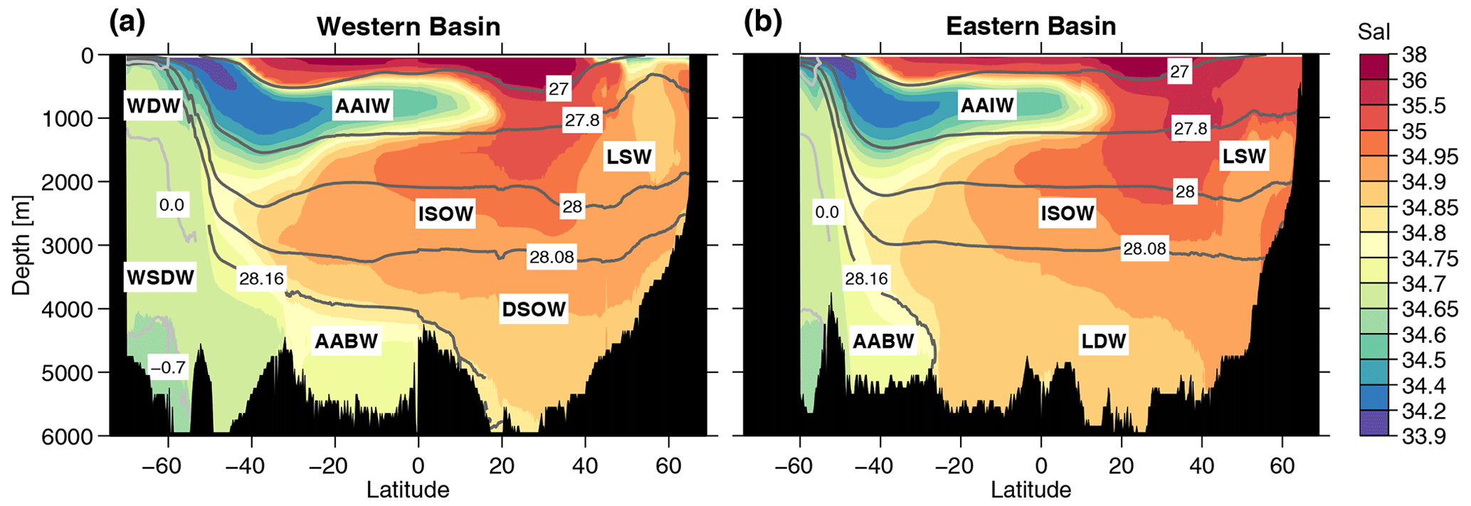
Figure 2 Zonal mean sections of salinity. (a) Western Atlantic basin, (b) eastern Atlantic basin. The contour lines show zonally averaged neutral density isopycnals γ_n (dark grey) and isotherms (light grey, θ = 0.0 °C and $\mathit{\theta }=-\mathrm{0.7}\mathrm{°}\mathrm{C}$, south of 50° S only) as boundaries of the main water masses. For abbreviations of water masses, see the text. Note the uneven spacing between contour intervals.

2.2 Major water masses and their definitions

The distribution of C_ant is inevitably linked to the spreading of the different water masses. We thus give a short overview of the major water masses in the Atlantic. The zonal mean salinity sections for the western and eastern Atlantic indicate the position of the main water masses (Fig. 2). The areas with high salinities reaching up to 400–600 m depth between 20–40° S and 20–40° N belong to the Subtropical Mode Waters (STMW). These are formed in the subtropical gyres by buoyancy loss and subduction (Talley, 1999). Further north in the eastern basin, the upper few hundred meters are covered by Subpolar Mode Water (SPMW) (Brambilla and Talley, 2008), which also has a relatively high salinity (> 35). The deeper region with salinities > 35.5 around 1000 m and 40° N in the eastern basin is dominated by the Mediterranean Outflow Water (MOW). As can be seen from the salinity distribution, this water mass penetrates further into the western basin and also mixes into the underlying North Atlantic Deep Water (NADW).

The low-salinity tongue at around 1000 m, stretching from 45° S–20° N, marks the Antarctic Intermediate Water (AAIW). This water mass is formed at the Subantarctic Front at about 45° S by ventilation of Subantarctic Mode Water (SAMW) formed in the southeastern Pacific and Drake Passage (McCartney, 1982). It even reaches the subpolar North Atlantic but loses its characteristic salinity minimum (Álvarez et al., 2004).

The most prominent deep water mass is the North Atlantic Deep Water, which consists of different components, i.e., Labrador Sea Water (LSW), Iceland–Scotland Overflow Water (ISOW) and Denmark Strait Overflow Water (DSOW). The LSW is formed in the northwestern subpolar North Atlantic by deep convection, occasionally reaching 2000 m depth (Lazier et al., 2023; Yashayaev, 2007; Kieke and Yashayaev, 2015). The salinity minimum associated with this newly formed LSW is clearly seen in Fig. 2a between 50 and 60° N. When spreading south- and eastward, the salinity of LSW increases due to mixing with surrounding more saline water masses, especially MOW.

The ISOW enters the subpolar North Atlantic via the Iceland–Scotland Ridge. It entrains ambient waters such as SPMW (Mauritzen et al., 2005), which leads to the relatively high salinity of this water mass (see the salinity maximum in Fig. 2b at 60° N between 2000 and 3000 m depth). Further downstream, the ISOW also entrains fresher LSW (Dickson et al., 2002), leading to a salinity decrease. Large parts of the ISOW enter the western basin mainly via the Charlie–Gibbs and Bight fracture zones (McCartney, 1992; Petit et al., 2018), while a smaller part continues southward in the eastern basin (Fleischmann et al., 2001).

The densest component of NADW is the DSOW. South of the Denmark Strait between Greenland and Iceland, this water spreads close to the bottom and entrains ambient waters (Jochumsen et al., 2015). It is less saline than the ISOW above. Due to its high density and great depth (below ≈3500 m), it cannot enter the eastern Atlantic directly.

In the Southern Ocean, NADW succumbs to upwelling and is incorporated into the Circumpolar Deep Water (CDW) (Iudicone et al., 2008). The southernmost extension of CDW between the Antarctic continent and the Antarctic Circumpolar Current is called Warm Deep Water (WDW). This water also contains older deep water from the other oceans and more recently ventilated water from the Weddell Sea in the Atlantic sector of the Southern Ocean (Klatt et al., 2002).

The water mass close to the bottom with relatively low salinity is the Antarctic Bottom Water (AABW). In the Atlantic, AABW is formed in the Weddell Sea, including subsurface excursions of saline shelf water below the ice shelf and substantial entrainment of WDW when descending into the abyss. It leaves the Southern Ocean, guided by topography, and enters into the deep basins of the western Atlantic (Bullister et al., 2013). Major pathways for deep and bottom waters to flow into the eastern basins are the Romanche Fracture Zone (Mercier and Morin, 1997) near the Equator and the Vema Fracture Zone at 11° N (Fischer et al., 1996). This eastward penetration of AABW at the Equator is visible by a salinity minimum directly above the bottom. The intensified vertical mixing with the overlying DSOW as observed in the Romanche Fracture Zone (Mercier and Morin, 1997) makes the bottom waters of the eastern basin more saline than in the western part. At the same time, the temperature increases, and the density decreases. This altered AABW in the eastern basin is then called Lower Deep Water (LDW). The further salinity increase in the deep eastern Atlantic towards the northern boundary might be explained by intrusion of the densest part of ISOW. Nevertheless, the influence of AABW is still visible, e.g., by enhanced noble gas concentrations observed along 60° N, originating from the entrainment of subglacial meltwater from the Antarctic ice shelves (Rhein et al., 2018).

South of the fronts of the Antarctic Circumpolar Current, at about 55° S, the densities of the deep water are considerably higher. There, the potential temperature θ is used to distinguish between Warm Deep Water (WDW; θ > 0 °C), Weddell Sea Deep Water (WSDW; 0 °C > θ > −0.7 °C) and Weddell Sea Bottom Water (WSBW; $\mathit{\theta }<-\mathrm{0.7}$ °C; van Heuven et al., 2011). WSBW, WSDW and WDW are precursor water masses of AABW.

The neutral density boundaries of some specific water masses are shown in all the figures of each section. We selected the boundaries according to the salinity distribution; i.e., the low-salinity tongue of the AAIW is comprised of the isopycnals γ_n = 27.0 and γ_n = 27.8 kg m⁻³. For the NADW components, we roughly follow the values given in Le Bras et al. (2017). Only for the density at the lower boundaries of LSW and ISOW do we use slightly denser isopycnals to better represent the salinity distribution. With the water mass boundaries shown in Fig. 2, the salinity minimum of the LSW in the northwestern Atlantic and the salinity maximum of the ISOW at the northern boundary of the eastern basin are completely contained in the respective water mass. For the boundary between DSOW and AABW, we chose the isopycnal γ_n = 28.16 kg m⁻³, almost following the isohaline S = 34.85. This leads to a northern boundary of AABW in the western basin at around 20° N. There are some extensions of AABW found further north, but they have mixed with the overlying DSOW and are thus more saline and also more enriched with anthropogenic tracers.

2.3 Anthropogenic carbon inferred from the TTD method

In this paper, we use a modified TTD method to infer the concentration of C_ant. This is based on the method used in Steinfeldt et al. (2009). In addition, we explicitly allow for the admixture of old, tracer-free waters. This approach has been used before, e.g., in Steinfeldt and Rhein (2004), but there it was locally restricted to the deep western boundary current in the tropics and was not used to calculate anthropogenic carbon. Here, we introduce a new algorithm that allows us to assign the admixture of old water at any location.

2.3.1 The standard TTD method

First, we explain the standard TTD method by following the procedure in Hall et al. (2002). Due to the advective–diffusive nature of oceanic transport, the water in the ocean interior consists of fluid elements with different pathways and ages (time elapsed since the water parcel left the mixed layer). The distribution of these ages, τ, is described by the TTD function 𝒢. The concentration of any conservative property C(x,t) at location x in the ocean interior and time t, which can be a particular reference year t_ref, is then given by (Hall et al., 2002)

$$\begin{array}{}\text{(1)}& C(x,t_{\mathrm{ref}})=\underset{\mathrm{0}}{\overset{\mathrm{\infty }}{\int }}{C}^{\mathrm{0}}(t_{\mathrm{ref}}-\mathit{\tau })\mathcal{G}(x,t_{\mathrm{ref}},\mathit{\tau })\mathrm{d}\mathit{\tau },\end{array}$$

where τ denotes the age of the water. C⁰(t) is the concentration history of the property in surface waters in the mixed layer. For upper water masses, we assume that C⁰(t) for CFCs and SF₆ is in solubility equilibrium with the atmosphere. For deeper, denser waters, the saturation gradually decreases to 80 %. A detailed list of the saturation used for each density layer is given in the supporting information in Table A1. In Steinfeldt et al. (2009), the minimum saturation was chosen to be lower, i.e., 65 %. However, CFC concentrations measured close to the formation region of NADW tend to be larger than 65 % of the surface saturation (see Fig. B1), so the value for the minimum CFC saturation has been enlarged for all dense water data. According to Steinfeldt et al. (2009), the difference in the inferred C_ant concentrations is about half the saturation difference; i.e., a saturation difference of 20 % leads to a C_ant difference of about 10 %. For C_ant, we use a time-independent carbon disequilibrium as in Waugh et al. (2006) and Steinfeldt et al. (2009). C_ant(t_ref) is calculated as the difference between the carbon concentration at time t_ref and the preindustrial time (year 1800). If the carbon disequilibrium remains constant, it cancels out when calculating this difference. At the beginning of the industrial period, atmospheric CO₂ increased by about 1 ppm per decade. This means an earlier or later start time for the beginning of the industrial period compared to 1800 would change the inferred C_ant concentration by about 0.6 µmol kg⁻¹ for the decades around 1800. As the Atlantic waters nowadays only contain a small fraction of water formed around the year 1800, the C_ant difference arising from a slightly different definition of the industrial period almost vanishes.

Equation (1) is used to infer concentrations of anthropogenic carbon (C_ant(x,t)) from the TTD functions $\mathcal{G}(x,t,\mathit{\tau })$. On the other hand, Eq. (1) allows us to infer the parameters of the TTD such that C(x,t) is the observed tracer concentration. To do so, a certain functional form of the TTD has to be assumed. Here, we apply an inverse Gaussian function as an approximation of the “real” TTD, as has been done in other studies (e.g., Hall et al., 2002; Waugh et al., 2006; Steinfeldt et al., 2009). This function only depends on two parameters: the mean age (mean value of τ) Γ (the first moment associated with the advective tracer transfer) and the width Δ (the second moment, which is related to the dispersion or mixing on all relevant scales, including recirculation and admixtures or entrainment of older water):

$$\begin{array}{}\text{(2)}& \mathcal{G}(\mathit{\tau },\mathrm{\Gamma },\mathrm{\Delta })=\sqrt{{\displaystyle \frac{{\mathrm{\Gamma }}^{\mathrm{3}}}{\mathrm{4}\mathit{\pi }{\mathrm{\Delta }}^{\mathrm{2}}{\mathit{\tau }}^{\mathrm{3}}}}}\exp \left({\displaystyle \frac{-\mathrm{\Gamma }(\mathit{\tau }-\mathrm{\Gamma }{)}^{\mathrm{2}}}{\mathrm{4}{\mathrm{\Delta }}^{\mathrm{2}}\mathit{\tau }}}\right).\end{array}$$

In order to derive both parameters (Δ and Γ), simultaneous measurements of different anthropogenic tracers are needed (Hall et al., 2002; Steinfeldt et al., 2009; Smith et al., 2011). As these are sparse, a fixed ratio of $\mathrm{\Delta }/\mathrm{\Gamma }$ is often used. This ratio is a measure of the importance of mixing (higher $\mathrm{\Delta }/\mathrm{\Gamma }$ values imply stronger mixing). Waugh et al. (2004) inferred a ratio of $\mathrm{\Delta }/\mathrm{\Gamma }=\mathrm{1}$ from tracer observations in the subpolar North Atlantic.

In an ideal case, if 𝒢 were the real TTD, the mean age Γ should be independent of the tracer from which it is inferred. Equation (1) then holds true for CFC-12, CFC-11, SF₆ and any other tracer taken from the same water sample with identical TTD parameters. In reality, if Eq. (1) holds true for one tracer (e.g., CFC-12) with the regional $\mathrm{\Delta }/\mathrm{\Gamma }$ value, applying Eq. (1) with the same parameters of 𝒢 to another tracer (e.g., CFC-11) may result in deviations of the order of a few percent from the observed CFC-11 concentration. In this study, we preferentially use CFC-12-derived ages; we use CFC-11 only when CFC-12 is not available. The number of the considered age data points is given in Table 1. CFC-12 and CFC-11 are the most commonly measured tracers (Table 2). The advantage of CFC-12 is that it increased in the atmosphere before CFC-11 and, in recent years, shows a smaller decline (Fig. C1). For young waters, this decline leads to relatively large errors (from measurement uncertainties and an unknown mixed-layer saturation) in the age and inferred anthropogenic carbon (Tanhua et al., 2008). Thus, for data after 2005 in the upper layers ($\mathrm{0}<{\mathit{\sigma }}_{\mathit{\theta }}<\mathrm{27.6}$ kg m⁻³) with young water (central and intermediate waters) and relatively high SF₆ concentrations, we use the SF₆-based age estimate, if available. If CFC-12 is measured simultaneously, it is used for the calculation of the $\mathrm{\Delta }/\mathrm{\Gamma }$ ratio. In the subpolar Atlantic north of 45° N, the density range for using the SF₆ age is expanded into the Labrador Sea Water, as here this water mass also has a relatively young age.

Steinfeldt et al. (2009) used pointwise TTDs with $\mathrm{\Delta }/\mathrm{\Gamma }$ ratios of 0.5, 1 or 2 for the subpolar to tropical Atlantic based on simultaneous observations of CFC-12/tritium and CFC-12/CFC-113. Here, we also make use of simultaneous measurements of CFC-12 and SF₆ to infer the $\mathrm{\Delta }/\mathrm{\Gamma }$ ratio and also round it to the quantized values of 0.5, 1 or 2. Note that SF₆ is not used at all in the deep and bottom waters, as the concentrations could still be enlarged from the remnants of artificial tracer release experiments in the 1990s in the Nordic Seas (Watson et al., 1999; Tanhua et al., 2005) and Brazil Basin (Polzin et al., 1997). Tritium is only used north of 45° N. This excludes southern sources with lower surface tritium values. Including those would imply a spatial dependence of C⁰ in Eq. (1), which is not applied here.

As in Steinfeldt et al. (2009), the inferred $\mathrm{\Delta }/\mathrm{\Gamma }$ ratios are gridded for each isopycnal layer in the same way as the other data (see Sect. 2.1). Due to the limited number of tritium, CFC-113 and SF₆ observations compared to CFC-12, the data from all 3 decades are combined, and any temporal change in the $\mathrm{\Delta }/\mathrm{\Gamma }$ ratio is not accounted for. The remaining data gaps of the gridded fields are filled with the standard value of $\mathrm{\Delta }/\mathrm{\Gamma }=\mathrm{1}$. The distribution of the resulting $\mathrm{\Delta }/\mathrm{\Gamma }$ ratios is shown in Fig. 3a and b for the western and eastern basins of the Atlantic. We find high ratios close to the maximum value of 2 at the surface and in the newly formed AAIW, NADW (LSW, ISOW, DSOW) and AABW. For the latter, the precursor water masses WSBW and WSDW directly north of Antarctica have a $\mathrm{\Delta }/\mathrm{\Gamma }$ ratio of approximately unity. Only the subtropical mode waters have $\mathrm{\Delta }/\mathrm{\Gamma }$ ratios below 1 near their formation region. Further downstream, the $\mathrm{\Delta }/\mathrm{\Gamma }$ ratio of the intermediate, deep and bottom waters decreases towards unity and even below, especially for LSW in the northeastern Atlantic.

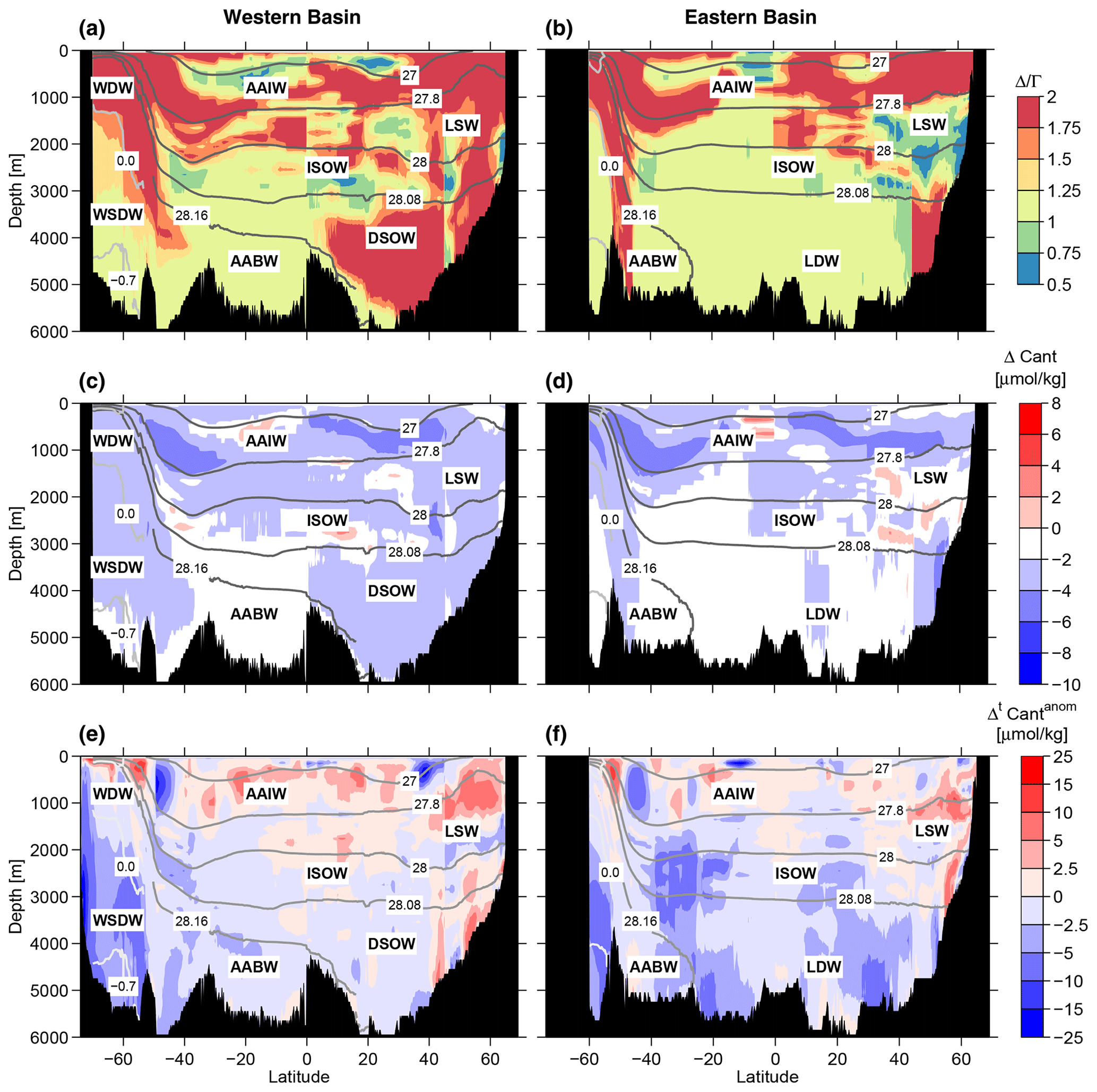
Figure 3 (a–b) Zonal mean sections showing the $\mathrm{\Delta }/\mathrm{\Gamma }$ ratio inferred from simultaneous observations of different tracers. (c–d) Difference in zonal mean C_ant concentrations calculated from a variable $\mathrm{\Delta }/\mathrm{\Gamma }$ ratio and from the constant ratio of $\mathrm{\Delta }/\mathrm{\Gamma }=\mathrm{1}$. The C_ant fields are based on tracer data from the whole period (1982–2021), and the reference year is 2020. (e–f) Zonal mean sections of ${\mathrm{\Delta }}_t{\mathrm{C}}_{\mathrm{ant}}^{\mathrm{anom}}$ for a variable $\mathrm{\Delta }/\mathrm{\Gamma }$ ratio (C_ant calculated for 2020 with data in 2020 minus C_ant calculated for 2020 based on tracer data in 1990, i.e., ${{\mathrm{C}}_{\mathrm{ant}}}^{\mathrm{2020}}-{{\mathrm{C}}_{\mathrm{ant}}}^{\mathrm{1990}\to \mathrm{2020}}$). Contour lines are shown as in Fig. 2. For details, see the text. Note the uneven breaks in the color scale.

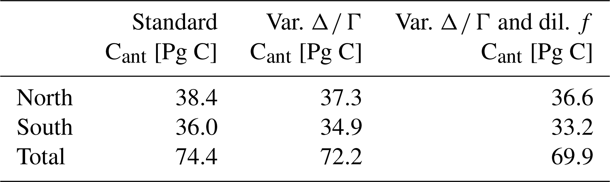
The difference between the C_ant concentrations based on the variable $\mathrm{\Delta }/\mathrm{\Gamma }$ ratio and the case that $\mathrm{\Delta }/\mathrm{\Gamma }=\mathrm{1}$ is depicted in Fig. 3c and d (here, the climatological C_ant fields referenced to 2010 are used). In general, $\mathrm{\Delta }/\mathrm{\Gamma }>\mathrm{1}$ leads to smaller values and $\mathrm{\Delta }/\mathrm{\Gamma }<\mathrm{1}$ to larger values of the inferred C_ant, as has also been found in He et al. (2018). The areas with $\mathrm{\Delta }/\mathrm{\Gamma }>\mathrm{1}$ dominate, but the basinwide reduction in the C_ant inventory due to the variable $\mathrm{\Delta }/\mathrm{\Gamma }$ ratio is only of the order of 1 Pg C (Table 3), both for the North Atlantic and the South Atlantic. In the study by He et al. (2018), the best agreement between the directly modeled global C_ant inventory and C_ant inferred from the TTD method is for a mean $\mathrm{\Delta }/\mathrm{\Gamma }$ ratio of 1.2, which is similar to our results for the Atlantic.

Table 3 Hemispheric and total Atlantic C_ant inventories referenced to 2010 for three different methods: the standard TTD method (as used, e.g., in Waugh et al., 2006), a variable $\mathrm{\Delta }/\mathrm{\Gamma }$ ratio (as used in Steinfeldt et al., 2009), and the modified TTD method with both a variable $\mathrm{\Delta }/\mathrm{\Gamma }$ ratio and an explicit dilution factor f.

One advantage of the TTD method is that it allows for choosing the reference year t_ref in Eq. (1). This makes it possible to group observations from several years to calculate C_ant for a common reference year, as has been done here for $\mathrm{CFC}/{\mathrm{SF}}_{\mathrm{6}}$ data from 1982–1994, 1995–2005, 2006–2013 and 2014–2021 and using all data from 1982–2021. By varying t_ref in Eq. (1), the TTD method also allows us to make predictions for future tracer concentrations. If the TTD parameters have been determined from a tracer observation at time t_obs, t_ref can be shifted into the future, and the concentration of any tracer can be inferred from Eq. (1) for this future time t_ref. The assumption underlying this prediction is that the TTD function 𝒢 remains the same, $\mathcal{G}(x,t_{\mathrm{obs}},\mathit{\tau })=\mathcal{G}(x,t_{\mathrm{ref}},\mathit{\tau })$; i.e., the ocean circulation and ventilation do not change. The increase in C_ant in this case is thus only due to the rising atmospheric CO₂. In particular, we use the tracer data from around 1990 (1982–1994) to predict C_ant for the reference year 2020. These predicted C_ant values are denoted by ${{\mathrm{C}}_{\mathrm{ant}}}^{\mathrm{1990}\to \mathrm{2020}}$. This prediction can be compared with the case where C_ant is inferred from data around the reference year. For example, ${\mathrm{C}}_{\mathrm{ant}}^{\mathrm{2020}}$ means C_ant is calculated from data between 2013–2021 and referenced to the year 2020. The difference, ${{\mathrm{C}}_{\mathrm{ant}}}^{\mathrm{2020}}-{{\mathrm{C}}_{\mathrm{ant}}}^{\mathrm{1990}\to \mathrm{2020}}$, can be interpreted as an anomaly in the C_ant increase (or accumulation) between 1990 and 2020 due to changes in the oceanic circulation/ventilation (i.e., in the TTDs) and is thus denoted as ${\mathrm{\Delta }}_t{\mathrm{C}}_{\mathrm{ant}}^{\mathrm{anom}}$, as in Gruber et al. (2019). These anomalies can also be inferred for the other decadal C_ant increase rates, i.e., ${{\mathrm{C}}_{\mathrm{ant}}}^{\mathrm{2000}}-{{\mathrm{C}}_{\mathrm{ant}}}^{\mathrm{1990}\to \mathrm{2000}}$ and ${{\mathrm{C}}_{\mathrm{ant}}}^{\mathrm{2010}}-{{\mathrm{C}}_{\mathrm{ant}}}^{\mathrm{2000}\to \mathrm{2010}}$.

Figure 3e–f show the distribution of ${\mathrm{\Delta }}_t{\mathrm{C}}_{\mathrm{ant}}^{\mathrm{anom}}$ for the western and eastern basins for the ${{\mathrm{C}}_{\mathrm{ant}}}^{\mathrm{2020}}-{{\mathrm{C}}_{\mathrm{ant}}}^{\mathrm{1990}\to \mathrm{2020}}$ case. The C_ant anomalies are discussed in detail in Sect. 3.3.2. Here, we only want to point out that in some cases large anomalies are found in the formation region of a water mass, e.g., for LSW and AAIW in the western Atlantic and, less pronounced, also in the eastern basin. The WSDW and AABW also exhibit large negative anomalies. Further downstream, in the equatorial region, the anomalies within LSW and AAIW are slightly smaller. This is to be expected, as away from the source region, waters from different vintages with different C_ant anomalies mix. However, we also find strongly negative values of ${\mathrm{\Delta }}_t{\mathrm{C}}_{\mathrm{ant}}^{\mathrm{anom}}$ in the LDW in the eastern Atlantic, which is the oldest water mass and not in the direct export pathway of AABW and DSOW. In these old waters, a pronounced C_ant anomaly should only occur for a pronounced longtime change in the ocean circulation and/or ventilation. But even then, the C_ant accumulation anomaly should be smaller than in the regions with high C_ant concentrations, like the water mass formation regions. Older waters contain a notable fraction with ages over 200 years (see the example in Table D1), i.e., C_ant free waters, which cannot contribute to the C_ant anomaly. We thus consider the strongly negative ${\mathrm{\Delta }}_t{\mathrm{C}}_{\mathrm{ant}}^{\mathrm{anom}}$ values in LDW as an artifact of the TTD parameterization in the form of a single inverse Gaussian function. In the next section we show how a modification of the TTD parameterization by including an additional dilution of young waters with old waters helps to overcome this artifact.

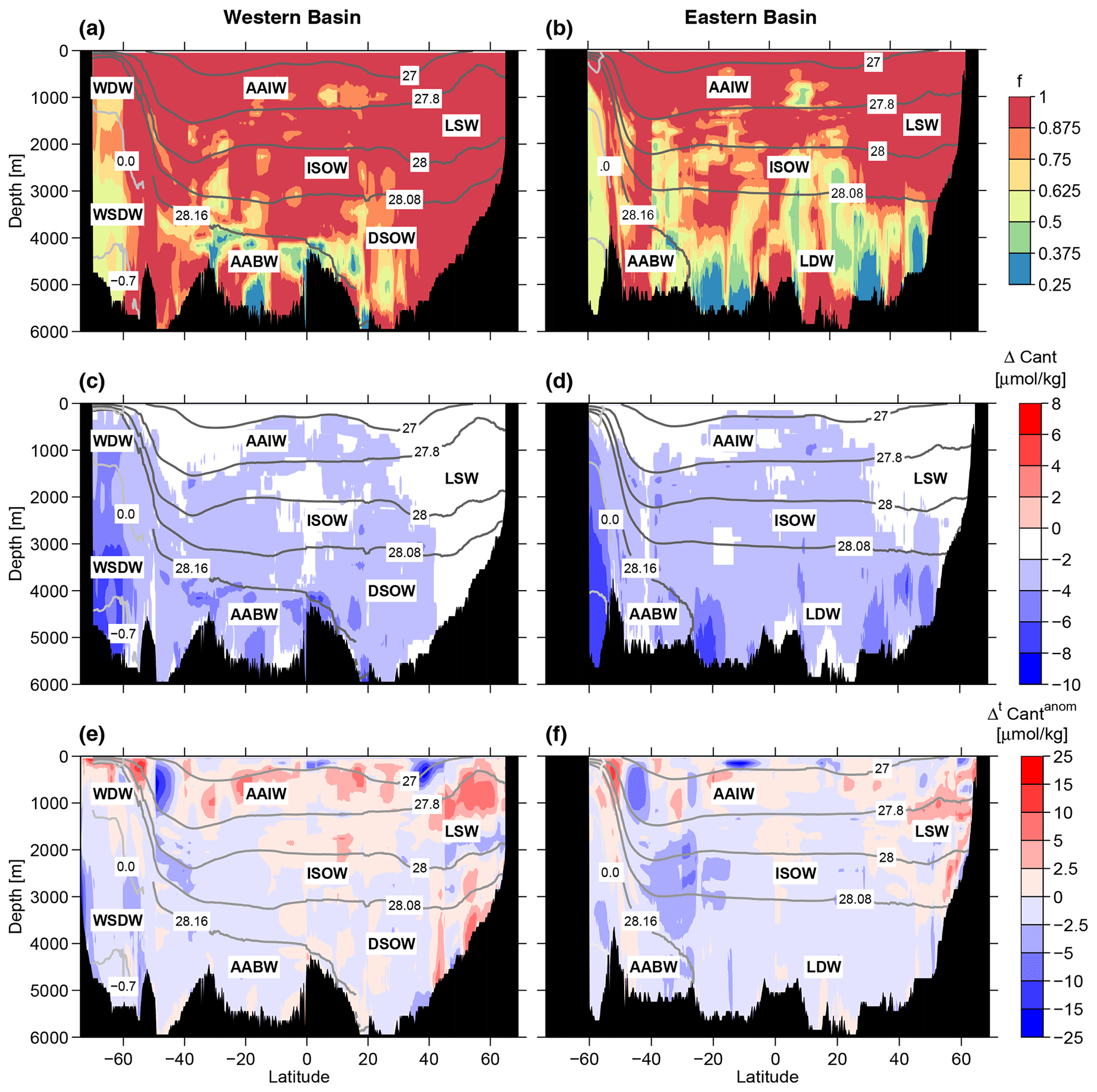
Figure 4 (a–d) Zonal mean sections showing the fraction f of young C_ant-bearing water. (c–d) Difference in zonal mean C_ant concentrations between the value calculated from a variable $\mathrm{\Delta }/\mathrm{\Gamma }$ ratio and no dilution and a variable $\mathrm{\Delta }/\mathrm{\Gamma }$ ratio with dilution. The C_ant fields are based on tracer data from the whole period (1982–2021), and the reference year is 2020. (e–f) Zonal mean sections of ${\mathrm{\Delta }}_t{\mathrm{C}}_{\mathrm{ant}}^{\mathrm{anom}}$ for a variable $\mathrm{\Delta }/\mathrm{\Gamma }$ ratio (C_ant calculated for 2020 with data in 2020 minus C_ant calculated for 2020 based on tracer data in 1990, i.e., ${{\mathrm{C}}_{\mathrm{ant}}}^{\mathrm{2020}}-{{\mathrm{C}}_{\mathrm{ant}}}^{\mathrm{1990}\to \mathrm{2020}}$). Contour lines are shown as in Fig. 2. For details, see the text. Note the uneven breaks in the color scale.

2.3.2 The modified TTD method with dilution

Steinfeldt and Rhein (2004) presented the foundation of the TTD method applied here by focusing on the Deep Western Boundary Current (DWBC) of the tropical Atlantic and investigating the NADW therein as a mixture of young and old water contributions. We apply the same principle here, but in contrast to the previous study, we extend this approach to the entire Atlantic Ocean.

$$\begin{array}{}\text{(3)}& \mathcal{G}=f\cdot {\mathcal{G}}_{\mathrm{young}}+(\mathrm{1}-f)\cdot {\mathcal{G}}_{\mathrm{old}}\end{array}$$

𝒢_old is assumed to not contain CFCs and also no C_ant; thus we do not need to consider it here. The additional parameter f describes the fraction of younger water and 1−f the dilution with old water. Eq. (1) then becomes

$$\begin{array}{}\text{(4)}& C\left(x,t_{\mathrm{ref}}\right)=\underset{\mathrm{0}}{\overset{\mathrm{\infty }}{\int }}{C}^{\mathrm{0}}\left(t_{\mathrm{ref}}-\mathit{\tau }\right)\cdot f\cdot {\mathcal{G}}_{\mathrm{young}}\left(x,t_{\mathrm{ref}},\mathit{\tau }\right)\mathrm{d}\mathit{\tau }.\end{array}$$

The dilution of younger water with an old component can be interpreted as follows: in the North Atlantic, the younger water can be interpreted as NADW and the old water as admixtures of AABW or recirculated NADW. In the South Atlantic, young waters are AABW and AAIW, and the old water originates from NADW. We also introduce an age threshold below which the dilution case is excluded. This is chosen as Γ_young = 100 years. Mean ages younger than 100 years only occur in and close to water mass formation regions, where a dilution with waters free of anthropogenic tracers is unlikely. Thus it is guaranteed that for these relatively young waters, e.g., in the vicinity of water mass formation regions where the temporal variability might be high, only the no-dilution case is applied.

In order to determine f, Steinfeldt and Rhein (2004) used assumptions that are only valid in the DWBC. Here, we want to apply the dilution in any region, especially for old water like the LDW, far away from the DWBC. The method used to determine the fraction f is as follows: for f = 1, we calculate C_ant as described above, with the $\mathrm{\Delta }/\mathrm{\Gamma }$ ratios determined from simultaneous observations of different transient tracers. In addition, we infer C_ant for values of f of 0.75, 0.5 and 0.25 with $\mathrm{\Delta }/\mathrm{\Gamma }=\mathrm{1}$. These quantized values are chosen to limit the computational effort and obtain marked differences between the derived C_ant concentrations. From the four sets of TTD parameters, four different C_ant values are inferred.

At each grid point, from these four TTD parameterizations, one is chosen that minimizes the C_ant differences between the climatology and the decadal values, i.e., min($\left({\mathrm{C}}_{\mathrm{ant}}\right(\mathrm{1982}-\mathrm{1994}{)}^{\mathrm{1990}}-{\mathrm{C}}_{\mathrm{ant}}(\mathrm{clim}{)}^{\mathrm{1990}}{)}^{\mathrm{2}}$ + $\left({\mathrm{C}}_{\mathrm{ant}}\right(\mathrm{1995}-\mathrm{2005}{)}^{\mathrm{2000}}-{\mathrm{C}}_{\mathrm{ant}}(\mathrm{clim}{)}^{\mathrm{2000}}{)}^{\mathrm{2}}+({\mathrm{C}}_{\mathrm{ant}}(\mathrm{2006}-\mathrm{2013}{)}^{\mathrm{2010}}-{\mathrm{C}}_{\mathrm{ant}}(\mathrm{clim}{)}^{\mathrm{2010}}{)}^{\mathrm{2}}$ + $\left({\mathrm{C}}_{\mathrm{ant}}\right(\mathrm{2014}-\mathrm{2021}{)}^{\mathrm{2020}}-{\mathrm{C}}_{\mathrm{ant}}(\mathrm{clim}{)}^{\mathrm{2020}}{)}^{\mathrm{2}}$), where, e.g., C_ant(1982−1994)¹⁹⁹⁰ means C_ant referenced to 1990 inferred from the decadal data from 1982–1994, and C_ant(clim)¹⁹⁹⁰ means the climatological C_ant value referenced to 1990. An example of the influence of varying the TTD parameters ($\mathrm{\Delta }/\mathrm{\Gamma }$ ratio, fraction f) on the shape of the TTD is given in Fig. D1.

The inferred fractions f are shown in Fig. 4a–b for the western and eastern basins. Close to the water mass formation regions, e.g., the subpolar North Atlantic, the waters are too young to allow for a dilution, so f is set to 1 there. The only exception is the WSDW, which has a dilution factor of about 0.5 adjacent to its formation region (the formation region itself at the Antarctic shelf is not considered here). A strong dilution with old waters (low f) is mainly found in the deep and bottom waters (AABW, LDW and DSOW south of 30° N). In these regions, the inferred C_ant concentrations are remarkably smaller than for the case without dilution (see Fig. 4c–d) by up to 10 µmol kg⁻¹. In general, the regions with f < 1 always show a reduction in C_ant. For the North Atlantic, where the regions with f = 1 dominate, the basinwide C_ant inventory is only reduced by 0.7 Pg C compared to the TTDs without dilution. For the South Atlantic, this reduction is larger (1.7 Pg C) (Table 3).

The introduction of the dilution f leads not only to smaller C_ant concentrations, but also to a reduction in the amount of the C_ant accumulation anomalies ${\mathrm{\Delta }}_t{\mathrm{C}}_{\mathrm{ant}}^{\mathrm{anom}}$. A comparison between Figs. 3e–f and 4e–f shows that ${\mathrm{\Delta }}_t{\mathrm{C}}_{\mathrm{ant}}^{\mathrm{anom}}$ becomes less negative, especially in the waters of Antarctic origin (WSDW, AABW and LDW), where f < 1. On the other hand, the positive C_ant anomalies in the NADW, especially the LSW, in the western tropical Atlantic hardly change; i.e., they are less dependent on the parameterization of the TTDs. In Sect. 3.3.2 we relate these C_ant accumulation anomalies with observed changes in ocean ventilation. As the spuriously negative values of ${\mathrm{\Delta }}_t{\mathrm{C}}_{\mathrm{ant}}^{\mathrm{anom}}$ in the old deep waters are reduced by taking into account the dilution of young water with old water, we use the modified TTDs with dilution to compute the Atlantic C_ant inventories. Another advantage of this TTD parameterization is that it reduces the relatively high C_ant concentrations in the Southern Ocean that result from the standard TTD method when compared to other C_ant calculation techniques (Waugh et al., 2006; Vázquez-Rodríguez et al., 2009; Khatiwala et al., 2013).

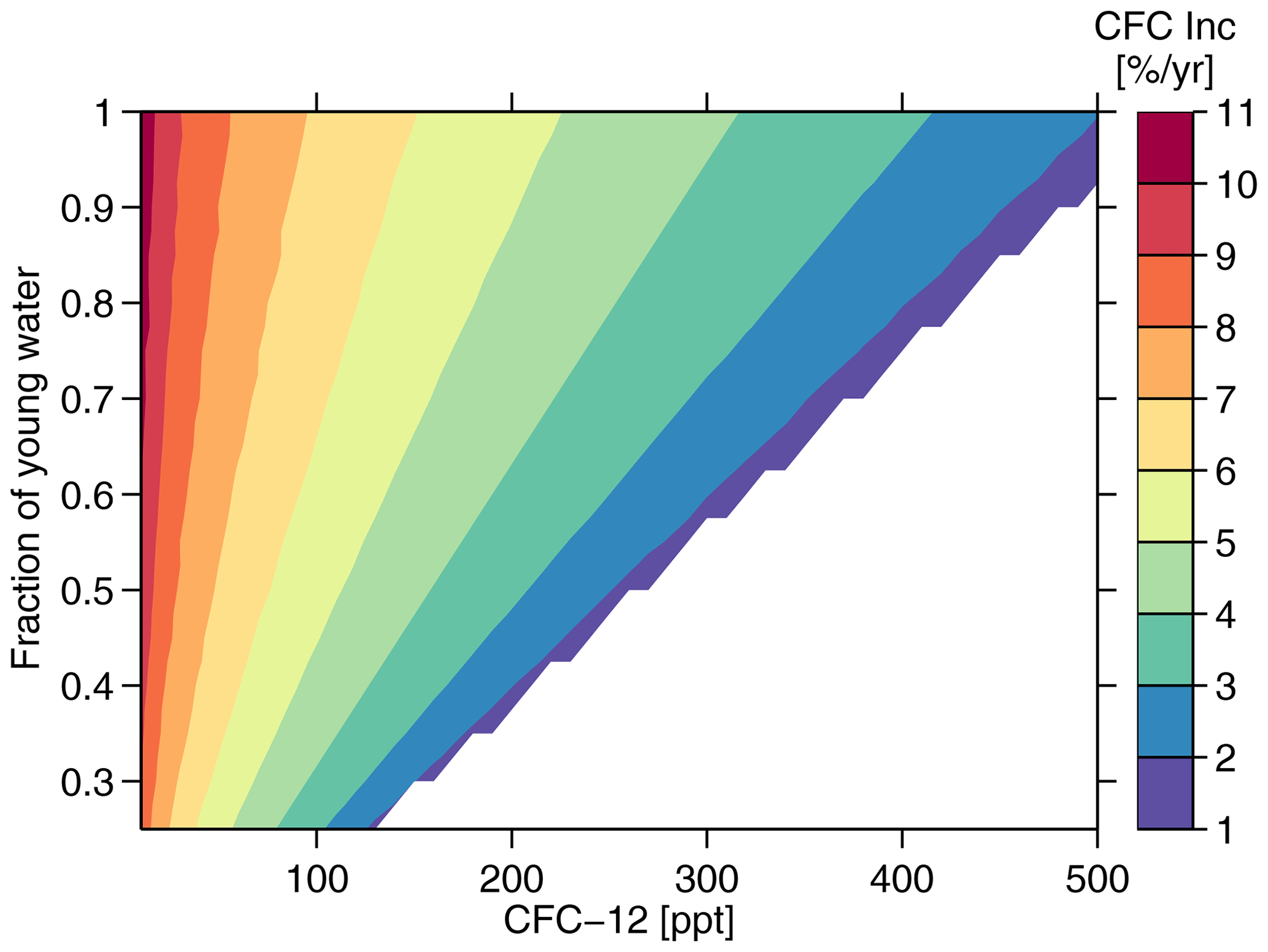
Figure 5 Expected increase rate (Inc) per year of CFC-12 for a concentration observed in the year 2000 as a function of the observed CFC-12 concentration itself and the fraction of young water. The increase is calculated from the TTDs inferred from the CFC-12 concentration in the year 2000, assuming a steady-state ocean. High CFC-12 concentrations are incompatible with low fractions of young water; thus, this area is left blank. For details, see the text.

The strongly negative C_ant accumulation anomalies, when using the standard TTDs, indicate that the water in 2020 is older than in 1990; thus C_ant calculated from the age in 1990 with the reference year 2020 is larger than C_ant derived from the age in 2020. Figure 5 shows that the CFC increase rate for a steady-state ocean (calculated from Eq. 1) CFC-12 in the year 2000 is smaller for smaller fractions f. If an observed CFC increase over time (around the year 2000) lags behind the expected value from Fig. 5, the water becomes older and vice versa. Thus the choice of the dilution factor f influences age changes inferred from observed temporal changes of the CFC-12 concentration. As a consequence, the magnitude of the C_ant anomaly ${\mathrm{\Delta }}_t{\mathrm{C}}_{\mathrm{ant}}^{\mathrm{anom}}$ also differs between different TTD parameterizations.

2.3.3 Error estimation

The error in C_ant is calculated similarly to Steinfeldt et al. (2009). The contributions of the interpolation/gridding error (3 %), the C_ant disequilibrium (possible undersaturation) (20 %) and the CFC disequilibrium (5.5 %, including errors in the CFC measurements) are treated the same. The C_ant uncertainty of 2.0 µ mol kg⁻¹ in very old waters (Steinfeldt et al., 2009) is considered to be a minimum error everywhere. If the CFC-12 concentration is below the typical detection limit of 0.005 pmol kg⁻¹, the C_ant concentration is set to zero. The error due to the TTD parameterization as an inverse Gaussian function compared to the real TTD is the maximum of the 20 % given in Steinfeldt et al. (2009) and the difference in C_ant calculated with the standard TTD method and the case with dilution. In the model study by He et al. (2018), the error arising from a change in the C_ant disequilibrium is relatively low (less than 10 % for all ocean regions), so our assumption might be an overestimation.

All these errors apply to the C_ant value at each data point. For the gridded fields, the statistical errors decrease according to the degrees of freedom, whereas the systematic errors remain unchanged. The errors due to the shape of the TTD and the unknown C_ant disequilibrium are assumed to be similar (or systematic) within one water mass, but they may vary between water masses. As there are about four different water mass classes (Central and Intermediate Water, LSW, Overflow Waters, and AABW), these errors are divided by $\sqrt{\mathrm{4}}=\mathrm{2}$ when the error for the total inventory is considered. The C_ant error of 2.0 µmol kg⁻¹ at low CFC concentrations can be regarded as cruise dependent. Most grid points are influenced by at least two cruises (e.g., a zonal and a meridional section). Thus, the error of 2.0 µmol kg⁻¹ is divided by $\sqrt{\mathrm{2}}$ for each grid point and by $\sqrt{n}$ for the whole inventory, where n denotes the number of cruises from which the gridded C_ant data are inferred.

For inventory differences in C_ant between times t₁ and t₂, the errors due to a change in C_ant and CFC disequilibria and the errors due to uncertainties in the TTD shape only have to be applied to the portion of C_ant that is added between t₁ and t₂. For the water formed prior to time t₁, which is still present at time t₂, these systematic errors mainly cancel each other out (Steinfeldt et al., 2009).

When comparing the predicted C_ant values for time t₂ based on observations at t₁ with the C_ant values based directly on observations at t₂, the error due to a change in the C_ant disequilibrium is neglected. The reason is that here we are interested in the effect of a change in age on the C_ant concentrations and not the effect of biogeochemical changes. Second, a change in the C_ant disequilibrium would affect the C_ant values for the prediction from observations at t₁ and from more recent observations at t₂ in a similar way.

3 Results and discussion

3.1 Basinwide C_ant distribution

The C_ant concentration and inventories of the Atlantic between 70° S and 65° N are computed for the reference years 1990, 2000, 2010 and 2020 from the decadal $\mathrm{CFC}/{\mathrm{SF}}_{\mathrm{6}}$ data. In addition, we use all data to calculate a quasi-climatological distribution of the Atlantic C_ant inventories for the same reference years. All inventories and their uncertainties are listed in Table 4. The Atlantic inventory of about 58.0 ± 9.3 Pg C in 2010 makes up 37 ± 9 % of the global C_ant storage (155 Pg C, best estimate in Khatiwala et al., 2013), whereas the fractional areal cover of the parts of the Atlantic considered here is only about 22 %.

Table 4 Atlantic C_ant inventories in petagrams of carbon (Pg C) for reference years 1990, 2000, 2010 and 2020 based on all tracer data and on tracer data from the decade centered around the reference year only.

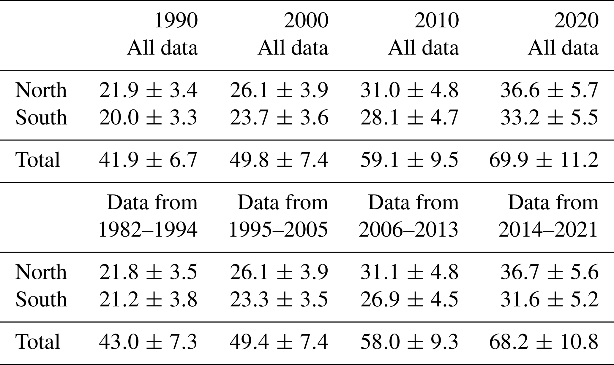
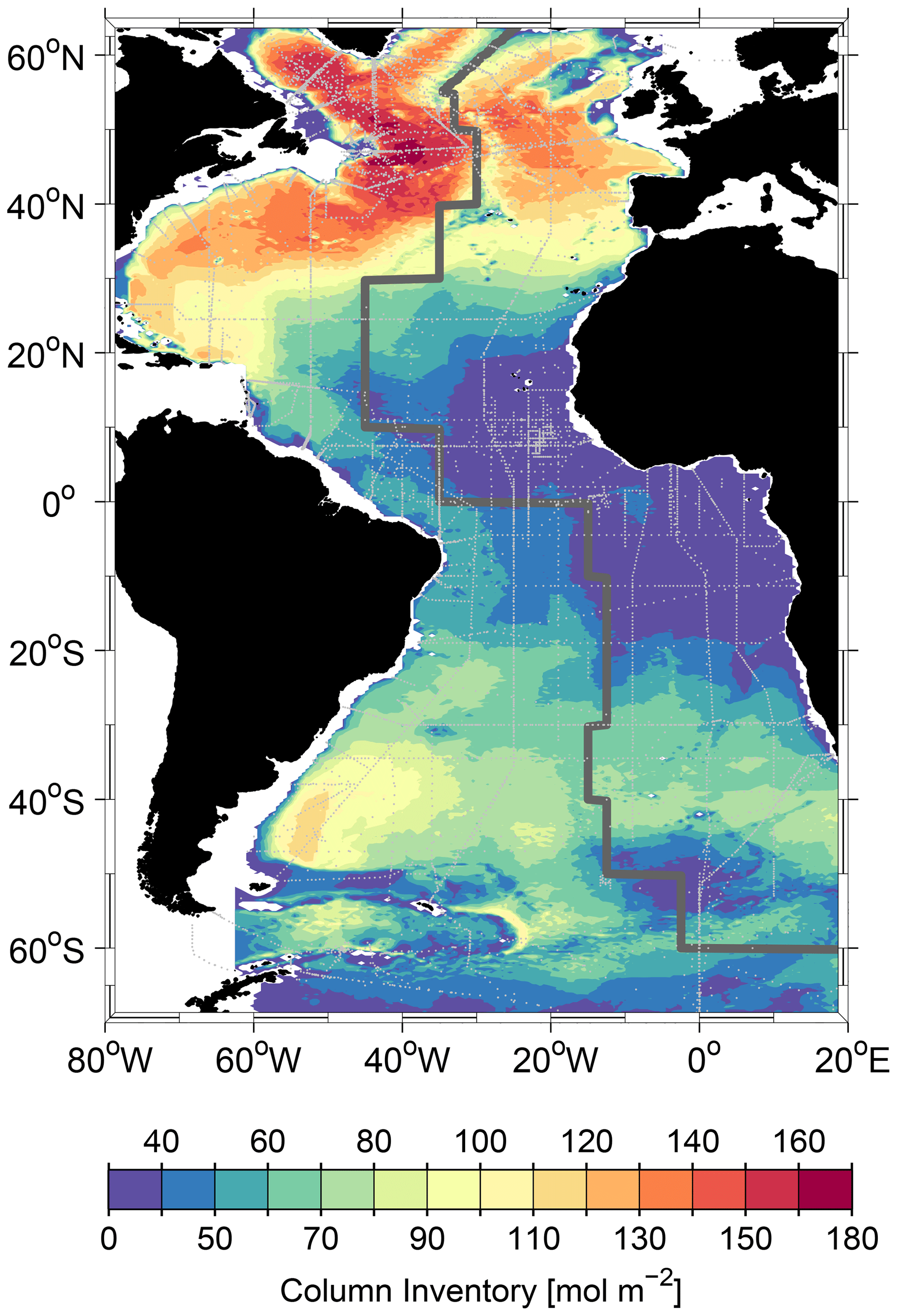
Figure 6 Map of the climatological C_ant column inventory referenced to 2020 based on all tracer data between 1982 and 2021. The thick line following the Mid-Atlantic Ridge indicates the boundary between the eastern and western basins. The dots indicate the locations of tracer samples used for the C_ant calculation. Note the uneven spacing between contour intervals at the beginning and end of the color scale.

The climatological column inventory obtained from the extended TTD method is shown in Fig. 6. A tongue of high-C_ant column inventories stretches southward from the C_ant maximum in the northwestern Atlantic towards the Equator. This reflects the southward propagation of NADW, mainly within the DWBC (Rhein et al., 2015). NADW is relatively high in C_ant compared to the deep water masses of southern origin.

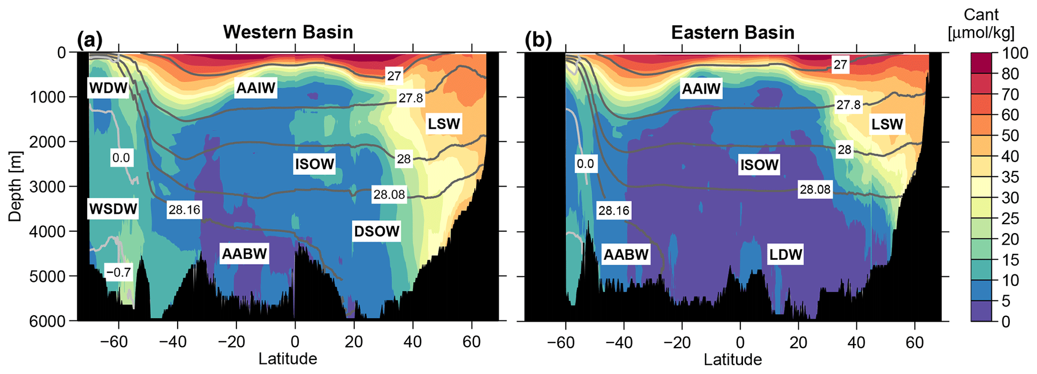
Figure 7 Zonal mean sections of C_ant referenced to 2020 based on all tracer data between 1982 and 2021. (a) Western basin, (b) eastern basin. Contour lines are shown as in Fig. 2.

The zonal mean sections for the eastern and western basins of the Atlantic, shown in Fig. 7, highlight the vertical C_ant distribution and the contributions of the different water masses to the column inventory. C_ant concentrations are high at the surface and in the central waters formed in the subtropical gyres. The maximum is found at the surface in the tropical/subtropical zone, where sea surface temperature (SST) is the highest. The reason is that the C_ant equilibrium concentration increases with temperature and alkalinity. The subtropical gyres in particular show high values of salinity and also alkalinity (Lee et al., 2006). The AAIW layer below forms a kind of transition zone between the C_ant-rich mode waters above and the C_ant-poor old deep waters below.

The most striking features in the deep waters are the elevated C_ant concentrations in the North Atlantic (Fig. 7). They are the highest in the western basin in the LSW layer, as this water mass is directly formed here (see Sect. 2.2). The spreading time for DSOW from its origin in the Nordic Seas towards the Labrador Sea is about 5 years (Rhein et al., 2015), resulting in lower C_ant concentrations. The NADW component with the lowest C_ant values is the ISOW, as this water mass has the longest travel time into the western Atlantic via the Charlie–Gibbs Fracture Zone (Smethie and Swift, 1989). The northeastern Atlantic generally exhibits smaller C_ant values in the deep waters. The LSW is also present there but with lower concentrations due to the spreading time of around 5 years from the formation region in the Labrador Sea towards the European continent (Sy et al., 1997; Yashayaev et al., 2007). The ISOW in the eastern basin does not reach the bottom of the deep basin, and the DSOW is not able to cross the Mid-Atlantic Ridge towards the east in the North Atlantic, so the deepest waters in the eastern basin (LDW) are low in C_ant. The southward spreading of NADW, mainly in the DWBC, leads to a tongue of enhanced C_ant concentrations in the western basin, which extends south of the Equator. The slightly enhanced concentrations in the LSW and AABW in the eastern equatorial Atlantic are due to the import of deep water from the western basin (Rhein and Stramma, 2005).

In the deep South Atlantic, C_ant in deep waters also decreases from west to east. The higher C_ant concentrations in the west are due to the spreading of AABW, which propagates from the Weddell Sea northward into the deep basins of the western Atlantic (Orsi et al., 1999). Another AABW branch continues eastward near 60° S. This branch can be seen in the enhanced C_ant values in Fig. 7a. It is also identified in the prime meridian section in Huhn et al. (2013) by the deep CFC-12 maximum. The C_ant concentrations in the AABW core are considerably smaller compared to NADW. Through the entrainment of old WDW (see Sect. 2.2), the transient tracer signal of AABW gets diluted, which explains the smaller C_ant values.

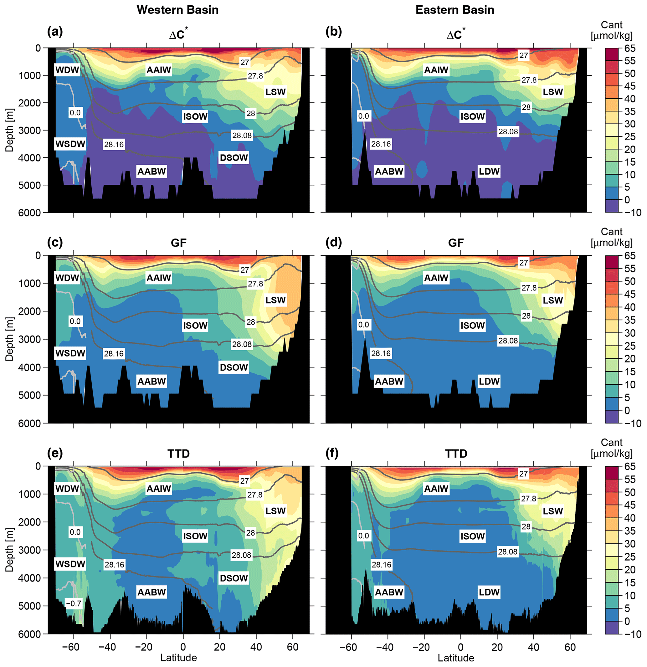
Figure 8 Zonal mean sections of C_ant referenced to 1994 from (a–b) the ΔC^∗ method (Sabine et al., 2004), (c–d) the GF method (Khatiwala et al., 2013) and (e–f) our TTD method. Contour lines are shown as in Fig. 2.

To compare our results directly with other methods, Fig. 8 shows the C_ant distributions in the western and eastern Atlantic from Sabine et al. (2004) (the ΔC^∗ method) and Khatiwala et al. (2013) (the Green function (GF) method). Here, all C_ant values are referenced to 1994. For our TTD-derived C_ant distribution we only use data from the first 2 decades (1982–2005) to have a data basis that is similar to that of the other studies. In the upper waters, the high C_ant concentrations in the Northern East Atlantic Central Water between 40 and 60° N from the ΔC^∗ method are distinct. Besides this, all methods yield similar results. This is different for the deep waters. There, the pattern of the C_ant distribution differs. The high C_ant concentrations in the cores of DSOW (between 40 and 60° N) and AABW (around 60° S) in the western basin can only be found using the TTD method. For the ΔC^∗ method, C_ant in the deep waters (ISOW, DSOW, LDW and AABW) is generally low and sometimes even has (unrealistic) negative values. For LSW, however, the results from the ΔC^∗ and TTD methods agree quite well. For this water mass, the GF method yields the highest concentration, especially in the western basin. Regarding the deeper water masses below the LSW, the results from the GF method are in between the ΔC^∗ and TTD values.

Overall, the improved TTD method used here leads to C_ant distributions that are compatible with the spreading of the water masses. The low C_ant values from the ΔC^∗ and GF methods in the recently formed DSOW and AABW are an unlikely scenario, as these water masses contain considerable amounts of CFCs (Smethie et al., 2000; van Heuven et al., 2011; Huhn et al., 2013), which have been in the atmosphere for a shorter time than C_ant.

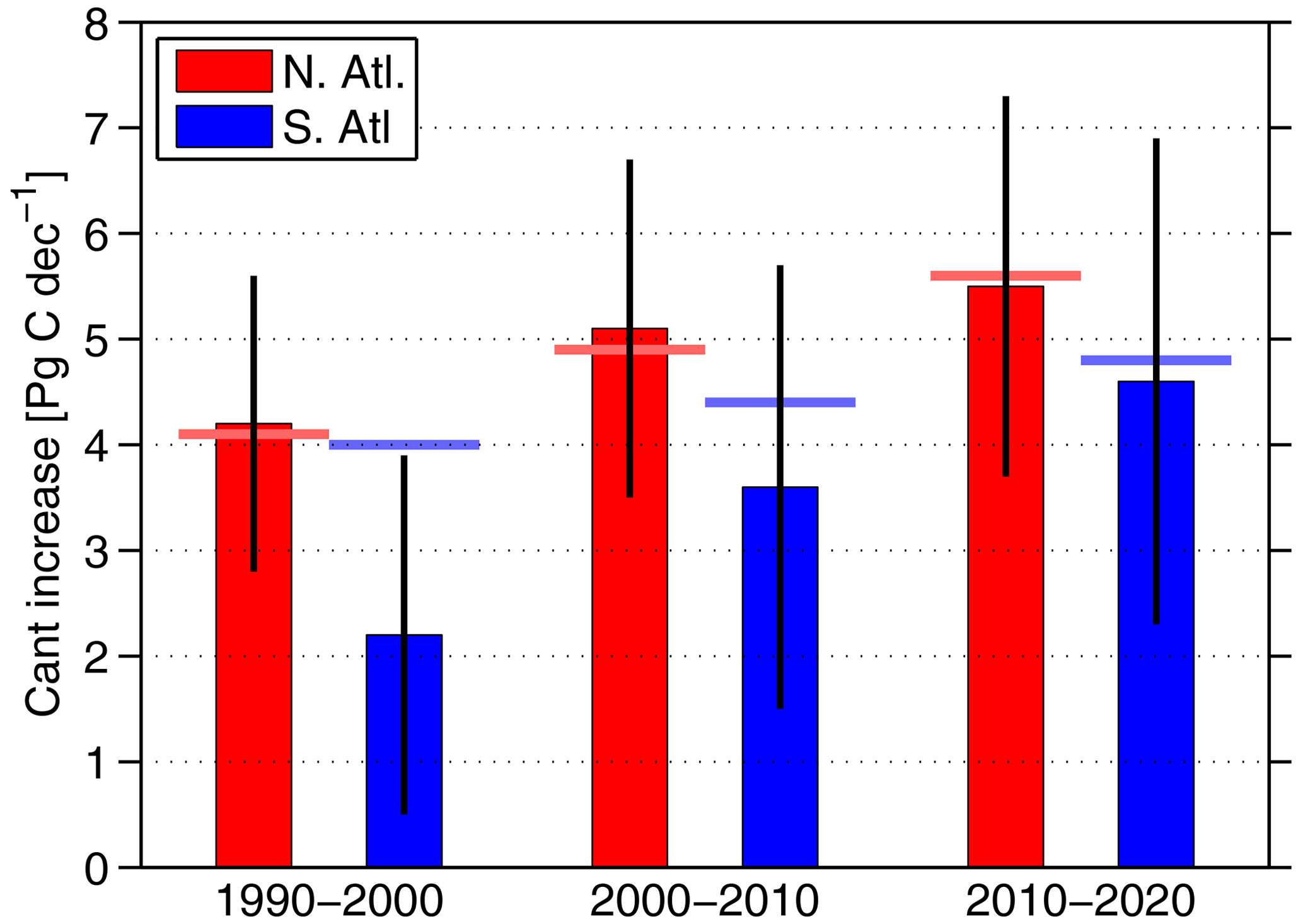
Figure 9 Decadal changes (1990–2000, 2000–2010 and 2010–2020) in the C_ant inventories for the North Atlantic (N. Atl.) and South (S. Atl.) Atlantic. The vertical black lines indicate the uncertainties. The horizontal colored lines show the inventory increase based on the C_ant inventory from the beginning of the decadal period (1990, 2000 and 2010) and a steady-state ocean circulation.

Woosley et al. (2016)Müller et al. (2023)

Table 5 Decadal changes in Atlantic C_ant inventories (Δ_tC_ant, in Pg C). The inventory differences are obtained from the decadal-data-only inventories listed in Table 3. They are compared with the values given in Woosley et al. (2016) (based on the eMLR method, the C_ant increase from 1990–2000 in Woosley et al., 2016, is adopted from Wanninkhof et al., 2010) and Müller et al. (2023) (eMLR(C^∗) method), where the increase is calculated for the periods of 1994–2004 and 2004–2014).

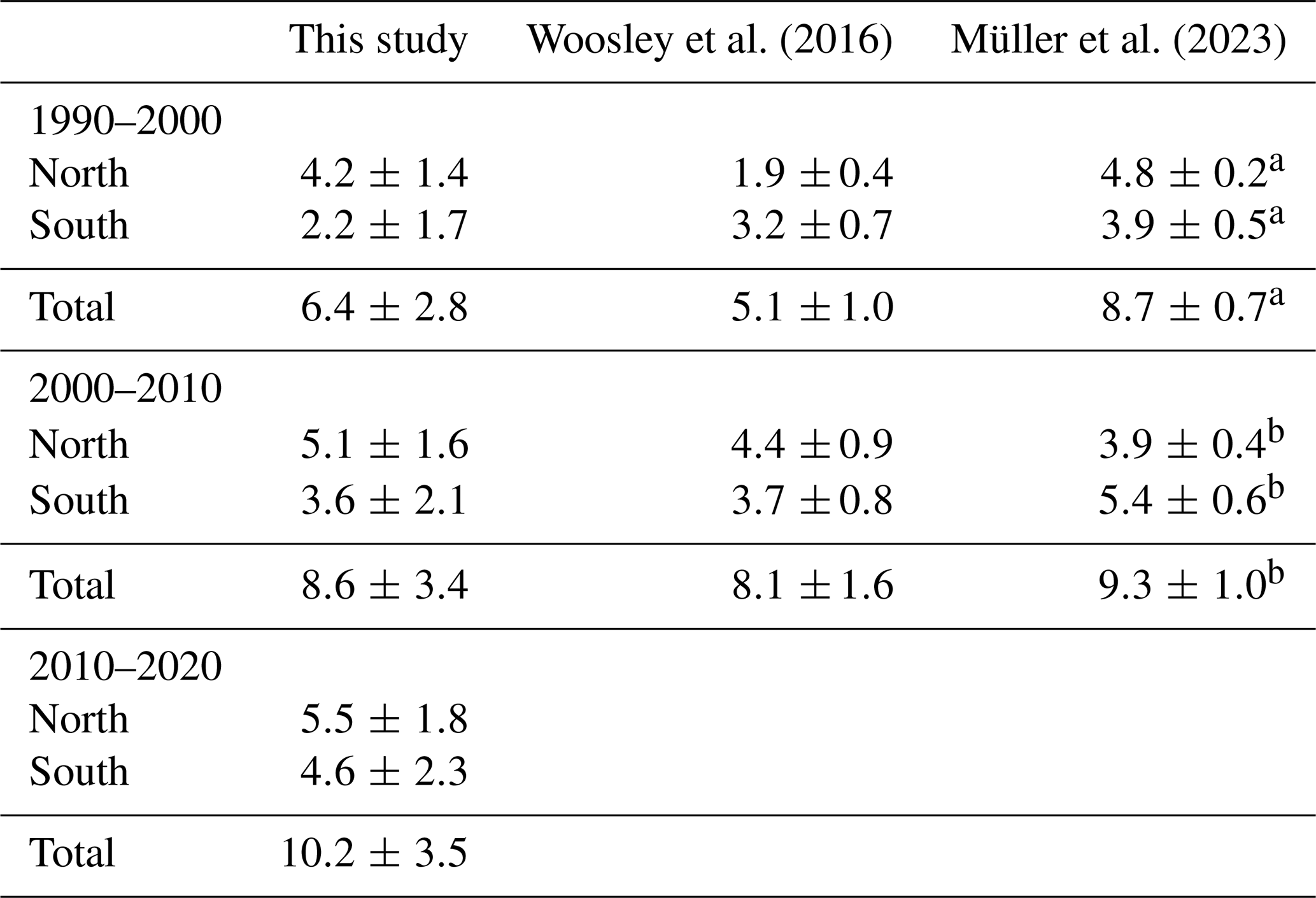
^a Value for the 1994–2004 period. ^b Value for the 2004–2014 period.

3.2 C_ant increase between 1990–2020

The decadal changes in C_ant inventories (Δ_tC_ant) are depicted in Fig. 9 and given in Table 5 together with results from other studies. Our results show a continuous increase in Δ_tC_ant over the 3 decades for both hemispheres. The North Atlantic shows higher C_ant storage compared to the southern part. This difference is most pronounced for the first decade from 1990–2000.

The inferred C_ant inventory changes from the other studies often show larger values of Δ_tC_ant in the South Atlantic and smaller ones in the North Atlantic compared to our result. This is especially the case for the 1990–2000 period in Woosley et al. (2016) (1.9 ±0.4 Pg C compared to 4.2 ± 1.4 Pg C in our study). The results in Woosley et al. (2016) are based on the eMLR method, and the values for the period of 1990–2000 are adopted from Wanninkhof et al. (2010). There, the C_ant change over the whole Atlantic is inferred from only one cruise, which, in the North Atlantic, is located in the eastern basin and hence does not cover the deep water formation areas in the Irminger and Labrador seas. This may introduce a bias into the results compared to our study. For the second period from 2000–2010, Woosley et al. (2016) use four cruises, also a small number compared to the number of cruises/data used in this study. Nevertheless, the agreement with Woosley et al. (2016) for the second decade is good (5.1 ± 1.6 Pg C vs. 4.4 ±0.9 Pg C). For the South Atlantic, the values in Woosley et al. (2016) are higher than ours, especially for the period of 1990–2000, but still agree within the error range.

By applying the eMLR(C^∗) method to inorganic carbon observations obtained from the previous version of GLODAPv2, Müller et al. (2023) infer the increase in the Atlantic C_ant inventory for the periods of 1994–2004 and 2004–2014. Unfortunately, these periods are shifted compared to ours by 4 years, which hampers direct comparison with our results. Due to the 4-year shift, the values in Müller et al. (2023) should be larger by about 8 % (see Sect. 3.3.2) if the ocean circulation were in a steady state. The most striking difference from our results is the decrease in Δ_tC_ant in the North Atlantic between the periods of 1994–2004 and 2004–2014. As in Woosley et al. (2016), the study by Müller et al. (2023) also yields higher C_ant storage rates in the South Atlantic compared to our results. Nevertheless, both Müller et al. (2023) and our results show a relatively large increase in this storage rate between the 1990s and 2000s.

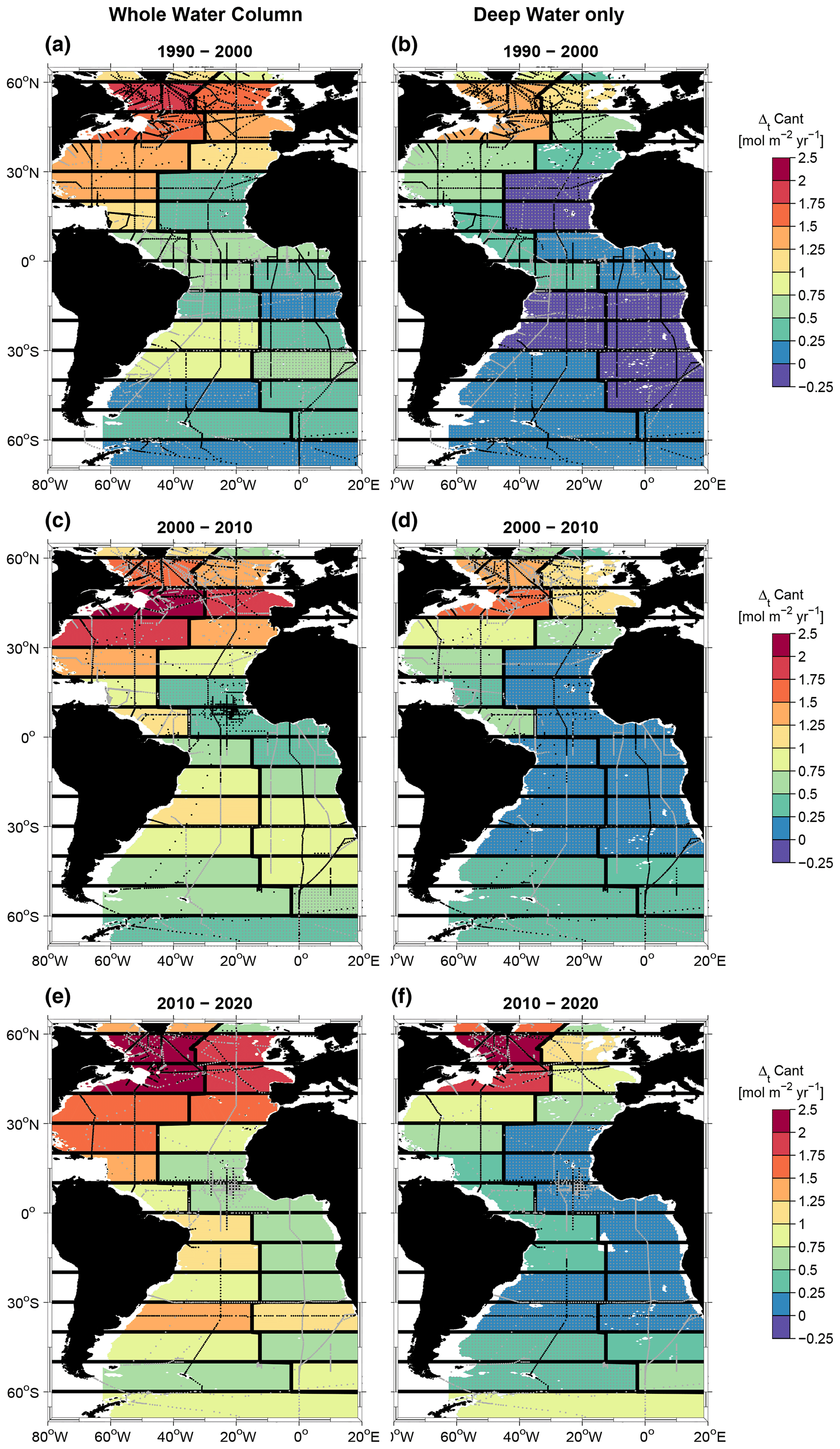
Figure 10 Mean C_ant storage rate (Δ_tC_ant) for the decades between 1990 and 2020 based on decadal data. Left column – whole water column, right column – only deep and bottom water masses. (a, b) 1990–2000, (c, d) 2000–2010, (e, f) 2010–2020. Only areas with a water depth larger than 200 m are considered. Station locations for the first period (1982–1994 in a, b; 1995–2005 in c, d; and 2006–2013 in e, f) are marked in light grey, and those for the second period (1995–2005 in a, b; 2006–2013 in c, d; and 2014–2021 in e, f) are marked in black. Regions with differences smaller than the error range are stippled.

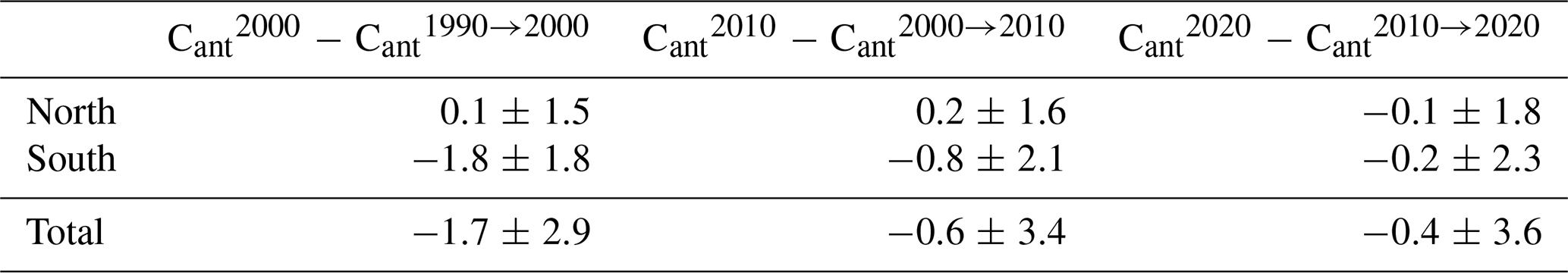
Table 6 C_ant accumulation anomalies for the Atlantic Ocean (${\mathrm{\Delta }}_t{\mathrm{C}}_{\mathrm{ant}}^{\mathrm{anom}}$), i.e., deviations between the C_ant increase based on tracer data from the actual period and the predicted C_ant increase based on tracer data from the previous period.

3.2.1 Local C_ant changes

We now discuss the decadal C_ant changes between 1990 and 2020 in different regions/water masses of the Atlantic. Figure 10 shows the mean annual storage rates for the respective decades between 1990 and 2020 over the whole water column (Fig. 10a, c, e) and the deep and bottom water layers only (Fig. 10b, d, f), which comprise the σ_1.5 and σ₄ layers from Table A1. Figure E1 shows the same C_ant changes as Fig. 10 but expressed as relative numbers. In Fig. 11 the changes in C_ant concentrations in the western and eastern basins are depicted. The C_ant increases shown in Figs. 10 and 11 reveal similar patterns to the C_ant distribution in Figs. 6 and 7; i.e., the C_ant increase over time is high when the C_ant concentration is also high. The largest increase appears close to the surface and in the subtropical mode waters, and the NADW also contributes significantly to the Atlantic C_ant storage. This becomes particularly evident when comparing the C_ant increase for the whole water column (Fig. 10a, c and e) with that for the deep and bottom waters only (Fig. 10b, d and f): in the subpolar North Atlantic, where the deep water layer extends close to the surface, the C_ant storage in deep and bottom waters alone is almost as large as for the total water column. The southward propagation of NADW in the western basin is reflected by a significant C_ant increase that extends to 10° S and is most pronounced in the LSW layer (Fig. 11a, c and e). In the eastern basin, any noticeable spatial C_ant increase in the younger NADW layer (LSW and ISOW) is limited to the region north of 30° N.

The deep and bottom waters in the Atlantic that are not influenced by younger NADW mainly show insignificant C_ant changes. South of about 40°S, the AABW exhibits a C_ant increase above the detection limit, at least in some places. These also contribute to the increase in the column inventory of the deep and bottom waters south of 40°S shown in Fig. 10f. The differences between the decadal C_ant storage rates are discussed in more detail in Sect. 3.3 on decadal variability.

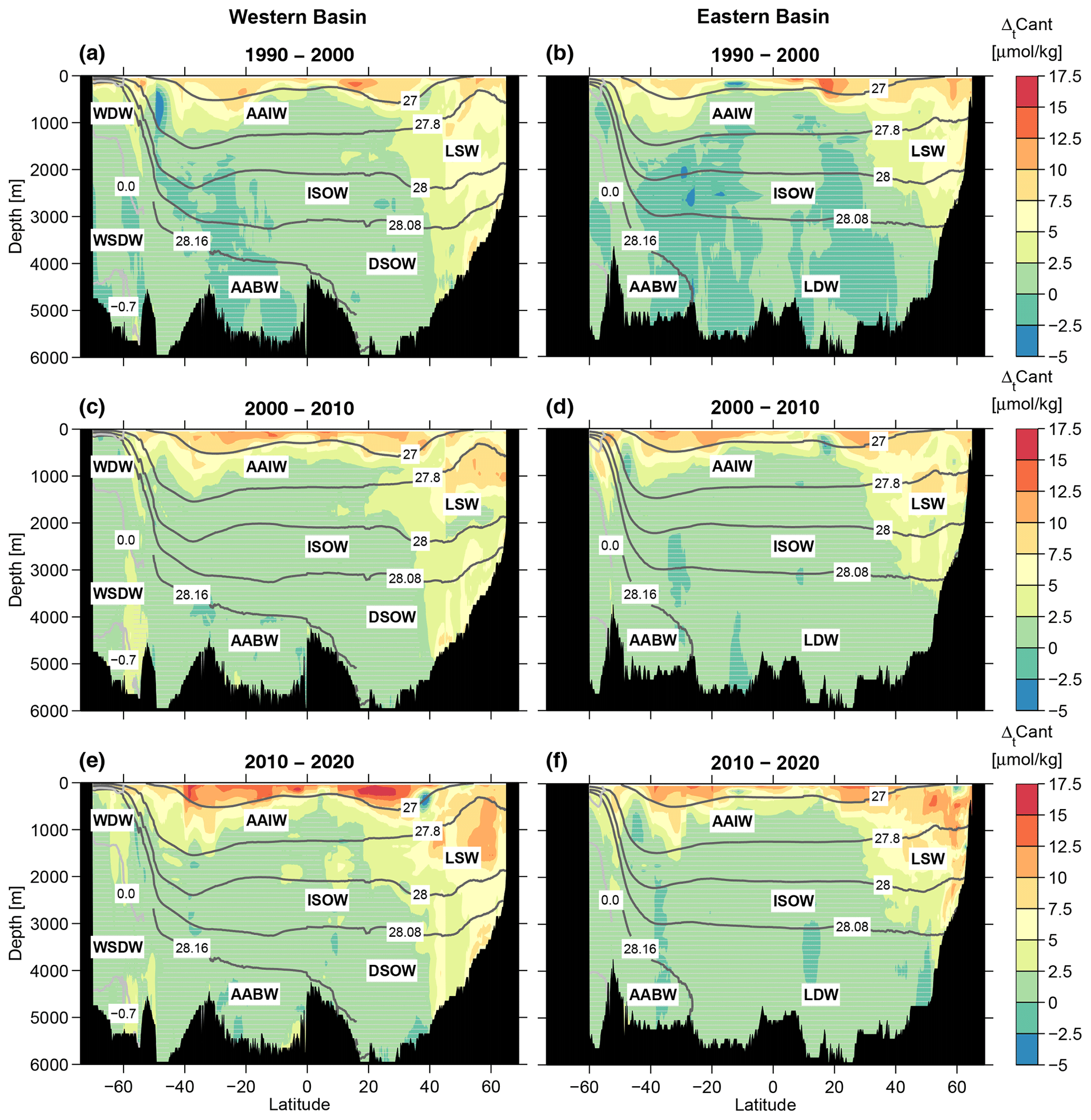
Figure 11 Zonal mean sections of C_ant concentration changes (Δ_tC_ant) based on decadal data for the periods between 1990 and 2010. (a, c, e) Western basin, (b, d, f) eastern basin, (a, b) 1990–2000, (c, d) 2000–2010, (e, f) 2010–2020. Regions with differences smaller than the error range are stippled. Contour lines are shown as in Fig. 2.

3.2.2 Comparison of local C_ant changes from the modified TTD method with dilution with other publications

We now compare our inferred local C_ant changes in the Atlantic with other published results. For the subpolar North Atlantic, the area with the highest increase in C_ant column inventory, Pérez et al. (2010) find similar storage rates (1.74 mol m² yr⁻¹ in the Irminger Sea and 1.88 mol m² yr⁻¹ in the Iceland Basin) to those shown in Fig. 10 but only from 1991–1997, where the North Atlantic Oscillation (NAO) was in a high phase. Afterwards, in the low-NAO period between 1997 and 2006, their rate is less than a quarter of the previous value (0.3–0.4 mol m² yr⁻¹). For the northeastern Atlantic, Pérez et al. (2010) also yield lower storage rates (0.72 mol m² yr⁻¹ for 1981–2006) compared to our analyses (> 1.0 mol m² yr⁻¹, Fig. 8a, c, d). In contrast to Pérez et al. (2010), our results are averaged over a larger region and also a longer time period (1 decade compared to 6 and 9 years in Pérez et al., 2010, for the Irminger Sea and Iceland Basin), which may lead to a damping of sudden, regional changes in the C_ant storage. However, the low C_ant increase in Pérez et al. (2010) after 1997 also points to methodological differences between the $\mathit{\phi }{\mathrm{C}}_T^{\mathrm{0}}$ method used in Pérez et al. (2010) and the modified TTD method with dilution used here. One of these is that the $\mathit{\phi }{\mathrm{C}}_T^{\mathrm{0}}$ method takes into account changes in the ocean air–sea CO₂ disequilibrium over time. On the other hand, a comparison of Fig. 11a and c indicates that in the 2000–2010 decade, the C_ant storage in the deeper part of the LSW is indeed very small (due to a reduction in the convection depth). The other water masses, however, i.e., the Overflow Waters and the waters above 1000 m, do not show a decrease in the C_ant uptake, in agreement with the ongoing renewal of these water masses. Thus, the small increase in the C_ant column inventory after 1997 in Pérez et al. (2010) seems to be unrealistic. Directly within the Labrador Sea, Raimondi et al. (2021) find a mean storage rate of 1.8 mol m² yr⁻¹ for the 1986–2016 period. The largest rates occur at the end of the time series and the smallest between 2005 and 2010. This is in good agreement with our findings (see Fig. 10a, c and d, the western box between 50 and 60° N).

In the western South Atlantic, the C_ant increase from our modified TTD method is similar to the results in Ríos et al. (2012) based on $\mathit{\phi }{\mathrm{C}}_{\mathrm{T}}^{\mathrm{0}}$. The C_ant storage is the highest in the Central Water, decreases downward with a minimum in the lower part of the NADW and shows some patches of significant C_ant increase towards the AABW near the bottom, south of 50° S (Fig. 11c). In the Weddell Gyre along the prime meridian, van Heuven et al. (2011) also find significant C_ant changes near the bottom. Applying the MLR method, they get an increase rate of 0.445 µmol kg⁻¹ per decade, whereas the trend in the directly observed carbon data is 1.15 µmol kg⁻¹ per decade. The latter compares well with our C_ant increase of about 1–2 µmol kg⁻¹ per decade (Fig. 11c), which is also supported by the study by Ríos et al. (2012), who yield a value of 0.15 µmol kg⁻¹ yr⁻¹. A full explanation for the discrepancy between the directly observed carbon increase and that derived from the MLR method is not provided by van Heuven et al. (2011). The comparison to our results supports their conclusion that the larger directly observed carbon trend could probably be ascribed primarily to the increase in C_ant, although the reason for the lower trend in the MLR results remains unexplained.

Müller et al. (2023) find the highest increase in the C_ant column inventory between 1994 and 2004 in the subtropical North Atlantic. The value of about 16 µmol m⁻² per decade is similar to our findings (Fig. 10), but our maximum in the subpolar western North Atlantic does not appear there. One reason could be that the column inventory in Müller et al. (2023) does not take into account waters below 3000 m depth to avoid the imprint of errors from the eMLR(C^∗) method. This implies that the C_ant-rich DSOW core in the western subpolar North Atlantic is missing in that study. For the second period (2004–2014) considered in Müller et al. (2023), the maximum of the increase in the C_ant column inventory is located in the western subtropical South Atlantic. The same holds true for the C_ant increase estimated in Gruber et al. (2019) for the 1994–2007 period, also based on the eMLR(C^∗) method. Our estimates of the C_ant column inventory always have their maximum in the western North Atlantic, either between 40 and 50° N or between 50 and 60° N (Fig. 10a, c and e).

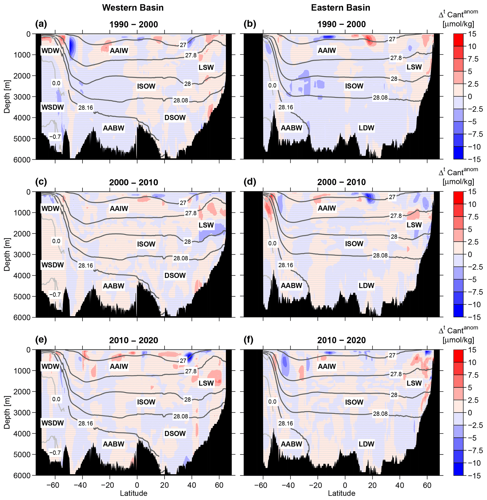
Figure 12 Zonal mean sections of ${\mathrm{\Delta }}_t{\mathrm{C}}_{\mathrm{ant}}^{\mathrm{anom}}$ (C_ant forecast based on tracer data from the first period minus C_ant based on tracer data from the second period). (a, c, e) Western basin, (b, d, f) eastern basin, (a, b) 1990–2000, (c, d) 2000–2010, (e, f) 2010–2020. Regions with differences smaller than the error range are stippled. Contour lines are shown as in Fig. 2. Note the uneven spacing between contour intervals.

In two recent studies by DeVries et al. (2023) and Pérez et al. (2024), the C_ant storage between 1994 and 2007 from Gruber et al. (2019) is compared with results from global ocean biogeochemical models and the ocean data assimilation model OCIM. Both types of models have the maximum of the C_ant storage in the subpolar North Atlantic and much smaller values than Gruber et al. (2019) in the subtropical South Atlantic. The spatial distribution of the modeled C_ant storage in DeVries et al. (2023) and Pérez et al. (2024) is thus qualitatively in better agreement with our results than compared with Gruber et al. (2019) and Müller et al. (2023).

3.3 Decadal variability of C_ant storage

As mentioned above, the TTD technique in general allows us to make predictions for C_ant concentrations based on older observations if one assumes a steady-state ocean; i.e., the TTD 𝒢 remains constant with time. In this case, the C_ant increase with time is solely due to the rising atmospheric CO₂. The TTD method thus allows us to distinguish between the C_ant variability generated by changes in oceanic circulation (which implies a change in the TTD) and the expected C_ant increase with time that merely results from the atmospheric CO₂ increase.

3.3.1 Evolution of C_ant for a steady-state ocean

We first consider the effect of the rising atmospheric CO₂ on the oceanic C_ant concentrations. If the mixed-layer concentration of the tracer C⁰ increases exponentially with time, $C^{\mathrm{0}}(t+\mathrm{\Delta }t)=C^{\mathrm{0}}\left(t\right)\exp \left(\mathit{\lambda }\mathrm{\Delta }t\right)$, then, following Eq. (1), the concentration of C in the ocean interior increases in the same way; i.e., $C(x,t+\mathrm{\Delta }t)=C(x,t)\exp \left(\mathit{\lambda }\mathrm{\Delta }t\right)$. Steinfeldt et al. (2009) applied an exponential fit of $C_{\mathrm{ant}}^{\mathrm{0}}\left(t\right)$ for the 1850–2003 time period and yielded a mean growing rate of 1.69 % yr⁻¹. Note that the increase rate of the equilibrium surface concentration $C_{\mathrm{ant}}^{\mathrm{0}}\left(t\right)$ is smaller by about 0.3 % yr⁻¹ than the change in C_ant in the atmosphere due to the nonlinear carbon chemistry. Small deviations of $C_{\mathrm{ant}}^{\mathrm{0}}\left(t\right)$ from the exponential fit cause the exact C_ant increase rate to depend on both the shape of the TTD (and thus the location) and the reference times for which C_ant is calculated. Here, we do not extend the exponential fit of ${\mathrm{C}}_{\mathrm{ant}}^{\mathrm{0}}\left(t\right)$ towards 2020 but infer mean decadal increase rates from the C_ant inventories in 1990, 2000, 2010 and 2020 based on all $\mathrm{CFC}/{\mathrm{SF}}_{\mathrm{6}}$ data (values in Table 3). The resulting increase is 1.74 % yr⁻¹ for the decade of 1990–2000, 1.73 % yr⁻¹ for 2000–2010 and 1.68 % yr⁻¹ for the last period of 2010–2020. All values are quite close to the result of 1.69 % yr⁻¹ in Steinfeldt et al. (2009). Gruber et al. (2019) also inferred an expected C_ant change based on the atmospheric CO₂ increase and mean changes in the buffer factor and C_ant disequilibrium. The resulting C_ant change between 1994 and 2007 was 28 %, or 1.92 % yr⁻¹. The higher value is probably because Gruber et al. (2019) considered only the atmospheric CO₂ increase between 1994 and 2007, which is larger than a longer-term mean, as the CO₂ growth rate has increased. However, the C_ant increase in the older waters in the ocean interior reflects the smaller rise in atmospheric CO₂ from earlier decades.

3.3.2 Deviations of C_ant storage from a steady state

Here, we come back to the C_ant accumulation anomalies ${\mathrm{\Delta }}_t{\mathrm{C}}_{\mathrm{ant}}^{\mathrm{anom}}$ that have been introduced in Sect. 2.3. The magnitude of these anomalies over the decades 1990–2000, 2000–2010 and 2010–2020 is presented in Table 6. It can also be inferred from Fig. 9 as the difference between the boxes and the horizontal colored lines, which show the C_ant increase based on the decadal forecasts (e.g., ${{\mathrm{C}}_{\mathrm{ant}}}^{\mathrm{1990}\to \mathrm{2000}}-{{\mathrm{C}}_{\mathrm{ant}}}^{\mathrm{1990}}$). In the South Atlantic, ${\mathrm{\Delta }}_t{\mathrm{C}}_{\mathrm{ant}}^{\mathrm{anom}}$ is negative, especially for the 1990–2000 period. This implies a decrease in C_ant storage due to changes in circulation and/or ventilation for the 1990–2000 decade compared to the period before 1990 and after 2000. Müller et al. (2023) also find a strong C_ant increase over the South Atlantic from their first (1994–2004) to their second decade (2004–2014). All other numbers in Table 6 are not significantly different from 0. Thus, at least for the Atlantic as a whole, the C_ant increase over the last 30 years is almost in agreement with the rising atmospheric CO₂. On smaller regional scales, however, there are regions where ${\mathrm{\Delta }}_t{\mathrm{C}}_{\mathrm{ant}}^{\mathrm{anom}}$ is statistically significantly different from 0 (Fig. 12). In general, the local extrema of ${\mathrm{\Delta }}_t{\mathrm{C}}_{\mathrm{ant}}^{\mathrm{anom}}$ are about ± 5 µmol kg⁻¹, the same magnitude as in Gruber et al. (2019).

The zonal mean section of the C_ant accumulation anomaly obtained for the western Atlantic for the periods of 1990–2000, 2000–2010 and 2010–2020 (Fig. 12a, c and e) shows some areas with extreme values of ${\mathrm{\Delta }}_t{\mathrm{C}}_{\mathrm{ant}}^{\mathrm{anom}}$ that are similar for all three decadal periods. One is located in the South Atlantic within the AAIW; one in the tropics (20° S–20° N) above the AAIW; and one in the North Atlantic in the Central Water, LSW, ISOW and DSOW.

The C_ant anomalies in the southwestern Atlantic are most pronounced over the first decade (1990–2000, Fig. 12a). They show negative values south of 40° S between 100 and 1000 m depth in the AAIW and positive anomalies directly south- and equatorward (south of 20° S) in a slightly shallower depth range within AAIW and the overlying SAMW. A similar structure has been inferred in Waugh et al. (2013) from transient tracer data for the southern parts of the Atlantic, Indian and Pacific oceans. These authors ascribe the changes in ventilation to a strengthening and southward movement of the westerly wind belt. This leads to enhanced upwelling of older water with low C_ant south of the polar front and increased northward Ekman transport and formation of mode waters (with high C_ant) north of the front. A similar dipole in the upper 1000 m of the South Atlantic is also evident in the study of Gruber et al. (2019). Tanhua et al. (2017) also found large C_ant storage in SAMW, at least between 1990 and 2005.

The second area with extreme values of ${\mathrm{\Delta }}_t{\mathrm{C}}_{\mathrm{ant}}^{\mathrm{anom}}$ in the tropical Atlantic is mainly restricted to the layer above 500 m (subtropical mode water). Positive and negative C_ant accumulation anomalies alternate in latitudinal direction and between the decades. They could be a consequence of variable mode water formation in the subtropics. Such changes in the subtropical cell with enhanced production and southward transport of C_ant-rich mode water have been inferred from an inverse model in DeVries et al. (2017) with enhanced production and equatorward transport of C_ant-rich mode water in the 1990s. Unfortunately, the study in DeVries et al. (2017) ended in 2010, and the decades in which the data are grouped are shifted by 5 years compared to our study, thus prohibiting a direct comparison of the decadal results. In contrast to our results, Gruber et al. (2019) find negative C_ant anomalies in the whole tropical Atlantic over the upper 1000 m.

The northernmost area with extreme values of ${\mathrm{\Delta }}_t{\mathrm{C}}_{\mathrm{ant}}^{\mathrm{anom}}$ is located north of 40° N in the subpolar North Atlantic, including the Labrador Sea (Fig. 12). This structure reflects the observed variability of convective activity in the Labrador Sea and the associated changes in LSW formation. An unprecedented deep-reaching convection formed a very dense mode of LSW from 1987 to 1994 (Yashayaev, 2007). During the following years, only lighter modes of LSW (Upper LSW, ULSW) have been formed (Stramma et al., 2004; Kieke et al., 2006; Yashayaev, 2007), whereas the pool of dense LSW (DLSW) has been exported from the formation region south- and eastward (Kieke et al., 2007; Rhein et al., 2015). These two processes are reflected in the positive ${\mathrm{\Delta }}_t{\mathrm{C}}_{\mathrm{ant}}^{\mathrm{anom}}$ for the 2000–2010 period around 1000 m (formation of ULSW modes) and the negative C_ant anomalies between 1500 and 2000 m (export of DLSW) in Fig. 12c. This lack of C_ant storage in the deeper part of the LSW between 2000 and 2010 is also visible in Fig. 11c.

In 2008, convection in the Labrador Sea exceeded a depth of 1600 m for the first time in years (Våge et al., 2009) but without a great impact on the C_ant and oxygen trends (Rhein et al., 2017). In the study by Gruber et al. (2019), the C_ant anomaly in the North Atlantic is negative down to a depth of ≈ 2500 m with the minimum in the upper ≈ 1000 m. Thus, a ULSW–DLSW dipole in C_ant is not found there. Studies on the convection in the Labrador Sea indicate that at least the upper 500–1000 m of the water column has been convectively renewed every year since the 1990s (Yashayaev, 2007; Kieke and Yashayaev, 2015; Yashayaev and Loder, 2016), which makes a drastic decrease in the C_ant storage in that depth range unlikely. Starting in 2014, deep-reaching convection in the Labrador Sea has re-emerged (Kieke and Yashayaev, 2015; Yashayaev and Loder, 2016). This is reflected by the positive C_ant anomaly in the LSW in the northwestern Atlantic between 2010 and 2020. However, the density of this recently formed LSW is still smaller than the density of the LSW originating from the early 1990s (Yashayaev and Loder, 2016). Hence, the positive ${\mathrm{\Delta }}_t{\mathrm{C}}_{\mathrm{ant}}^{\mathrm{anom}}$ values do not reach the lower boundary of the LSW layer. The Irminger Sea has also been influenced by the enhanced deep convection in the subpolar northwestern Atlantic, and a large increase in C_ant has been found there (Fröb et al., 2016).

In the bottom waters north of 40° N (DSOW), there is an alternating pattern of negative and positive ${\mathrm{\Delta }}_t{\mathrm{C}}_{\mathrm{ant}}^{\mathrm{anom}}$ values (Fig. 12a, c and e). From 1965–2000, the overflow waters experienced a freshening trend lasting more than 3 decades (Dickson et al., 2002). This long-term trend does not influence the C_ant uptake of ISOW and DSOW, as no such signal is evident in Fig. 12. Annual fluctuations in salinity (and also temperature) for the DSOW particularly coincide with the long-term freshening trend (Yashayaev, 2007). These different vintages of DSOW might be the reason for the alternating minima and maxima in ${\mathrm{\Delta }}_t{\mathrm{C}}_{\mathrm{ant}}^{\mathrm{anom}}$ in the bottom waters north of 35° N.

In the northeastern Atlantic, the C_ant accumulation anomaly in the LSW for the 2000–2010 period is similar to that in the northwestern part, although less pronounced. LSW is formed in the western Atlantic, and the ${\mathrm{\Delta }}_t{\mathrm{C}}_{\mathrm{ant}}^{\mathrm{anom}}$ of the newly formed LSW becomes diluted when the anomalies spread eastward. The recent positive ${\mathrm{\Delta }}_t{\mathrm{C}}_{\mathrm{ant}}^{\mathrm{anom}}$ value in LSW did not become prominent in the eastern North Atlantic until 2020.

Another small region with a C_ant deficit is located within the deep and bottom waters (WSDW and AABW) of the southwestern Atlantic around 55° S between 1990 and 2000. This is the area where the newly formed deep water originating from the Weddell Sea is advected eastward (see above). This recently ventilated WSDW is relatively high in C_ant (Fig. 7a) but only shows a small decadal increase (Fig. 12a), lacking the expected growth from the atmospheric CO₂. This result is in agreement with Huhn et al. (2013), who also found an aging and ${\mathrm{\Delta }}_t{\mathrm{C}}_{\mathrm{ant}}^{\mathrm{anom}}$ deficit of AABW in the Weddell Sea. After 2000, this negative anomaly does not occur anymore, and the C_ant increase in WSDW/AABW between 60 and 50° S is higher (Figs. 11c, e and 12c, e).

Negative C_ant accumulation anomalies can also be found in the southeastern Atlantic between 2000 and 3000 m depth and from 45 to 25° S in the 1990–2000 period. As this negative anomaly is far away from the deep water formation regions, we have no clear explanation for this. One reason could be that the waters present in 1990 are still affected by the Weddell Polynya that occurred in the years 1974, 1975 and 1976 (Carsey, 1980) and are thus relatively high in C_ant.

4 Summary and conclusions

We used a modified TTD method allowing for the admixture of old, C_ant-free waters to access the C_ant inventory of the Atlantic, its increase and its variability over the last 2 decades. In 1990, 43.0 ± 7.3 Pg C of C_ant was stored in the whole Atlantic. Over the next 30 years, this amount increased to 68.2 ± 10.8 Pg C. This increase is mainly caused by the rising atmospheric CO₂ concentrations. Changes in circulation/ventilation have a regional impact on the C_ant concentrations but only a minor effect on the basinwide inventory.

The absolute C_ant inventories seem to be similar across the most common methods, like the ΔC^∗, TTD and GF methods, except for some subregions like the Southern Ocean, where the TTD method yields larger values. However, the incorporation of an explicit dilution into the TTD method leads to C_ant concentrations that are smaller by more than 5 µmol kg⁻¹ in parts of the WSDW and AABW compared to the TTD method without dilution, thus reducing the deviations from the other methods. Still, discrepancies between the different C_ant calculation techniques occur in the vertical distribution of C_ant, especially regarding the C_ant fraction of the deep ocean. This has repercussions for the conclusions on how well and for how long C_ant is stored in the ocean. Larger C_ant storage in deep waters with a long turnover time compared to upper water masses will remove C_ant from the atmosphere more enduringly.

Our C_ant increments of 6.4 ± 2.8, 8.6 ± 3.4 and 10.2 ± 3.5 Pg C for the 3 decades are about 30 %–40 % of the global values of 2.0 ± 0.5, 2.1 ± 0.5 and 2.5 ± 0.6 Pg C yr⁻¹ in Friedlingstein et al. (2020). The Atlantic area considered here constitutes 22 % of the global ocean area. The high C_ant concentrations in the North Atlantic due to NADW formation lead to the high contribution of the Atlantic to the global C_ant storage compared to its areal fraction.

The main discrepancy between this study and others using the eMLR (Woosley et al., 2016) and eMLR(C^∗) method (Gruber et al., 2019; Müller et al., 2023) is the regional distribution of the C_ant change. Some of the differences can be explained by the inefficiency of the non-TTD methods in resolving the C_ant changes in the deep ocean. In the global studies by Gruber et al. (2019) and Müller et al. (2023), the increase in the C_ant column inventory in the Atlantic still exceeds that in the Pacific and Indian oceans, but the global maximum in the North Atlantic is missing. Applying our TTD method, we find a significant C_ant increase in the overflow waters (ISOW and DSOW) in the North Atlantic, which contributes to the increase in the column inventory there. In contrast, in Woosley et al. (2016) the deep layers of the North Atlantic are found to be almost stagnant in C_ant, and in Gruber et al. (2019) and Müller et al. (2023) the C_ant increase below 3000 m depth is only considered for the total inventory, not for the C_ant distribution. The significant increase in the C_ant concentrations in ISOW and DSOW found in our study has not been reported before. Evident through the presence and temporal increase in CFCs in these overflow waters, it is unlikely that these waters have not contributed to the storage of C_ant over the last 2 decades.

Moreover, the C_ant accumulation anomaly due to a variable ocean circulation in Gruber et al. (2019) opposes our findings. In Gruber et al. (2019), this anomaly is mainly positive in the South Atlantic, except for the AAIW layer, and negative in the North Atlantic. In our study, the deep South Atlantic shows a slightly negative C_ant accumulation anomaly, and in the North Atlantic, we find alternating patterns with a positive anomaly in ULSW and negative in DLSW between 2000 and 2010. Using the standard TTDs instead would lead to an even larger C_ant deficit in the South Atlantic (see Figs. 3e and f and 4e and f) due to the higher “expected” CFC increase with time (Fig. 5).

The patterns of the C_ant accumulation anomalies found here mainly follow the changes in water mass age and ventilation that have already been described in previous studies, e.g., for the Southern Ocean (Waugh et al., 2013; Huhn et al., 2013), and the changes in the convective activity in the Labrador Sea (Kieke et al., 2007; Yashayaev, 2007; Yashayaev and Loder, 2016). All these studies are based on the variability of hydrographic properties and/or anthropogenic tracers. The large C_ant accumulation anomaly in the old waters of the South Atlantic, as found in Gruber et al. (2019), is not reflected in hydrographic changes. On the one hand, the old part (prior to the CFC input into the atmosphere) of our TTDs is not well constrained; hence some unresolved temporal variability might exist. On the other hand, enhanced variability in old waters is unlikely, as property anomalies in the ocean are typically large near the water mass formation regions and decay downstream towards the old waters in the ocean interior.

The investigation of oceanic circulation and ventilation variability and its impact on anthropogenic carbon storage is important for understanding the mechanisms behind the recent variability in oceanic carbon uptake (DeVries et al., 2019) and for estimating the future evolution of the oceanic carbon sink in a changing climate. Our results show that a decoupling of the atmospheric C_ant increase and the increase in the Atlantic C_ant storage has not yet been achieved by the observed decadal variability in water mass ventilation and circulation.

Appendix A: Isopycnal interpolation of profiles

The boundaries for the isopycnal interpolation of the single profiles, as described in the main text, are given in Table A1. For most of the cruises used here, CTD data (temperature and salinity data with a vertical resolution of 1 to 2 dbar) would also be available. However, we decided to retain the bottle data from GLODAPv2.2023 for salinity and potential temperature and to infer the layer thicknesses. One reason is that in GLODAP salinity and thus density are also quality controlled. We calculated the difference between the layer thicknesses inferred from CTD and bottle data for a cruise where both are available. The root-mean-square error of the layer thicknesses is about 40 m. If one assumes a maximal C_ant difference over this depth range of about 20 µmol kg⁻¹ (from Fig. 6), the difference in the C_ant column inventory would be ≈ 40 m × 20 µmol kg⁻¹ × 1000 kg m⁻³ = 0.8 mol m⁻², which is about 1 % of the total C_ant column inventory (see Fig. 5, between 30 and 180 mol m⁻²). The error in the layer thicknesses is randomly distributed (in some cases the layer with the higher C_ant concentration is too thick; in other cases it is too thin). Due to the large number of profiles (> 1000), the total error is much smaller than 1 %.

Table A1 Boundaries of density layers and assumed saturation for CFCs and SF₆ in every layer.

Appendix B: CFC and SF₆ saturation

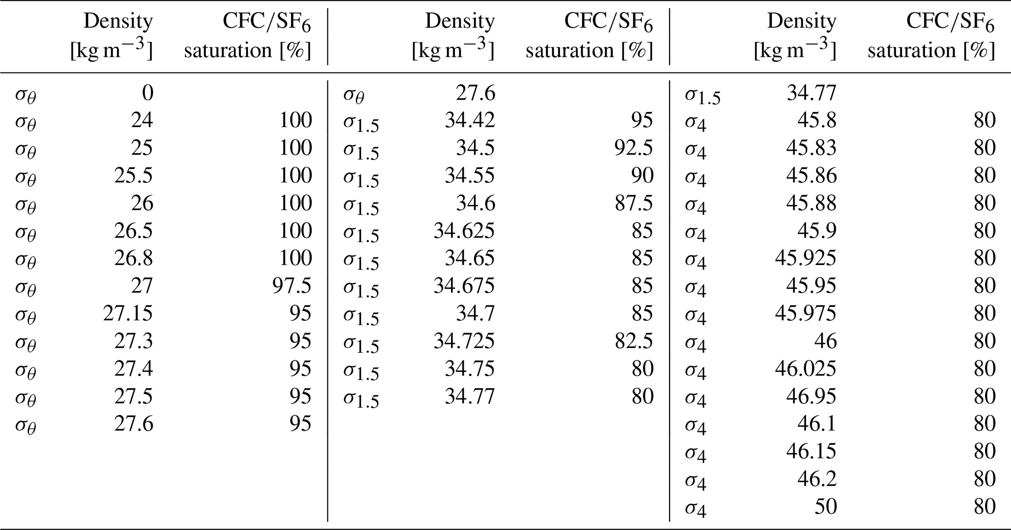
The CFC and SF₆ saturations assumed for the different density layers are given in Table A1. They decrease from 100 % in the upper waters to 80 % in deep waters. For most cruises, the surface is close to saturation, both for CFCs and for SF₆. Hence, a saturation of 100 % for the upper layers seems to be reasonable. For the deep layers, the saturation of the surface waters at the time of deep water formation, i.e., late winter/early spring, needs to be known. However, most cruises from higher latitudes are from late spring until autumn, avoiding the severe winter conditions. In order to estimate the saturation of newly formed North Atlantic Deep Water, Fig. B1 shows the CFC-12 and SF₆ data from the western subpolar North Atlantic (Labrador Sea and Irminger Sea respectively) below 500 m depth for 2 different years, expressed as saturation with respect to the solubility equilibrium. This has been calculated by using the observed potential temperature and salinity as well as the atmospheric tracer concentration from the year of observation. Waters with the highest saturation point to remnants from the last winter convection; waters with lower saturations are a mixture of recently ventilated and older water. This interpretation is different from that of Raimondi et al. (2021), where the mean tracer concentration in the core layer of newly formed LSW after convection is used to infer the saturation.

In 1994, mainly the denser mode of LSW had been ventilated, between σ_1.5=34.65 and σ_1.5=34.7 kg m⁻³. In 2013, the ventilation only reached densities above σ_1.5=34.6 kg m⁻³. The highest saturations in the ventilated density range are between 80 % and 100 % for both years. The SF₆ saturation in 2013 is only slightly below the values for CFC-12.

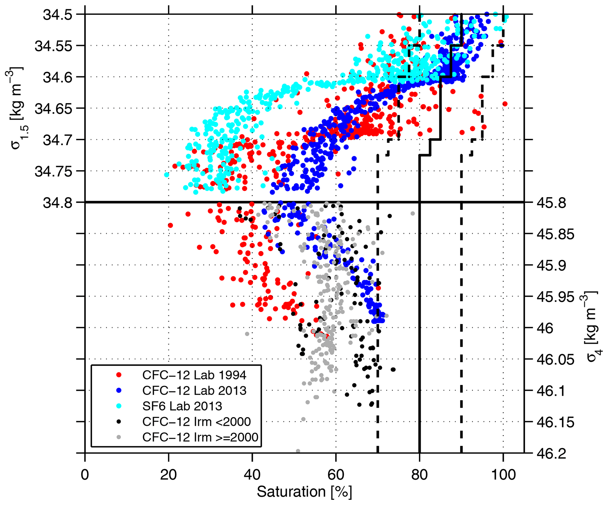
Figure B1 CFC-12 and SF₆ data below 500 m from the Labrador Sea (years 1994 and 2013) and the Irminger Sea (years prior to and after 2000), expressed as saturation with respect to the actual solubility equilibrium. Also shown is the assumed tracer saturation and the error margin of ± 10 %.

The overflow waters are not directly formed in the subpolar North Atlantic but originate from the Nordic Seas. However, they are modified after passing the Greenland–Scotland Ridge; e.g., the ISOW entrains Labrador Sea Water and Northeast Atlantic Water (LeBel et al., 2008), and the DSOW entrains warm and saline Atlantic Water and fresher water from the East Greenland Current (Jochumsen et al., 2015). The tracer saturation of the overflow waters (σ₄ >45.8 kg m⁻³) in the Irminger Sea, downstream of the entrainment, is shown in Fig. B1 for data prior to and after the year 2000. The saturation is even higher for the earlier period, probably due to short-term variability of the properties of the overflow waters (Yashayaev, 2007; Jochumsen et al., 2015). The maximum is around 80 %, but most data points have a smaller saturation. Note, however, that the Irminger Sea is located downstream of the formation area; hence the overflow waters there are not newly formed but have already been subject to aging and dilution, which reduces the apparent CFC saturation. In Fig. B1 the tracer saturation from Fig. A1 is also depicted, including the assumed error of 10 %. The saturation of 85 % for the major part of the LSW density range is identical to the value used in Kieke et al. (2006), Kieke et al. (2007) and Steinfeldt et al. (2009). For the DSOW, the applied saturation of 80 % is significantly larger than the 65 % from Steinfeldt et al. (2009) but close to the value of 75 % from Swift et al. (1980) and LeBel et al. (2008).

Appendix C: Temporal evolution of anthropogenic tracers

Figure C1 shows the concentration of CFC-11, CFC-12 and SF₆ in the northern hemispheric atmosphere and tritium in North Atlantic surface waters as a function of time. The tritium curve for the North Atlantic from Dreisigacker and Roether (1978) is continued assuming radioactive decay after 1978. Atmospheric CFC and SF₆ concentrations are adopted from Bullister (2015) and extrapolated linearly in time for the last 5 years.

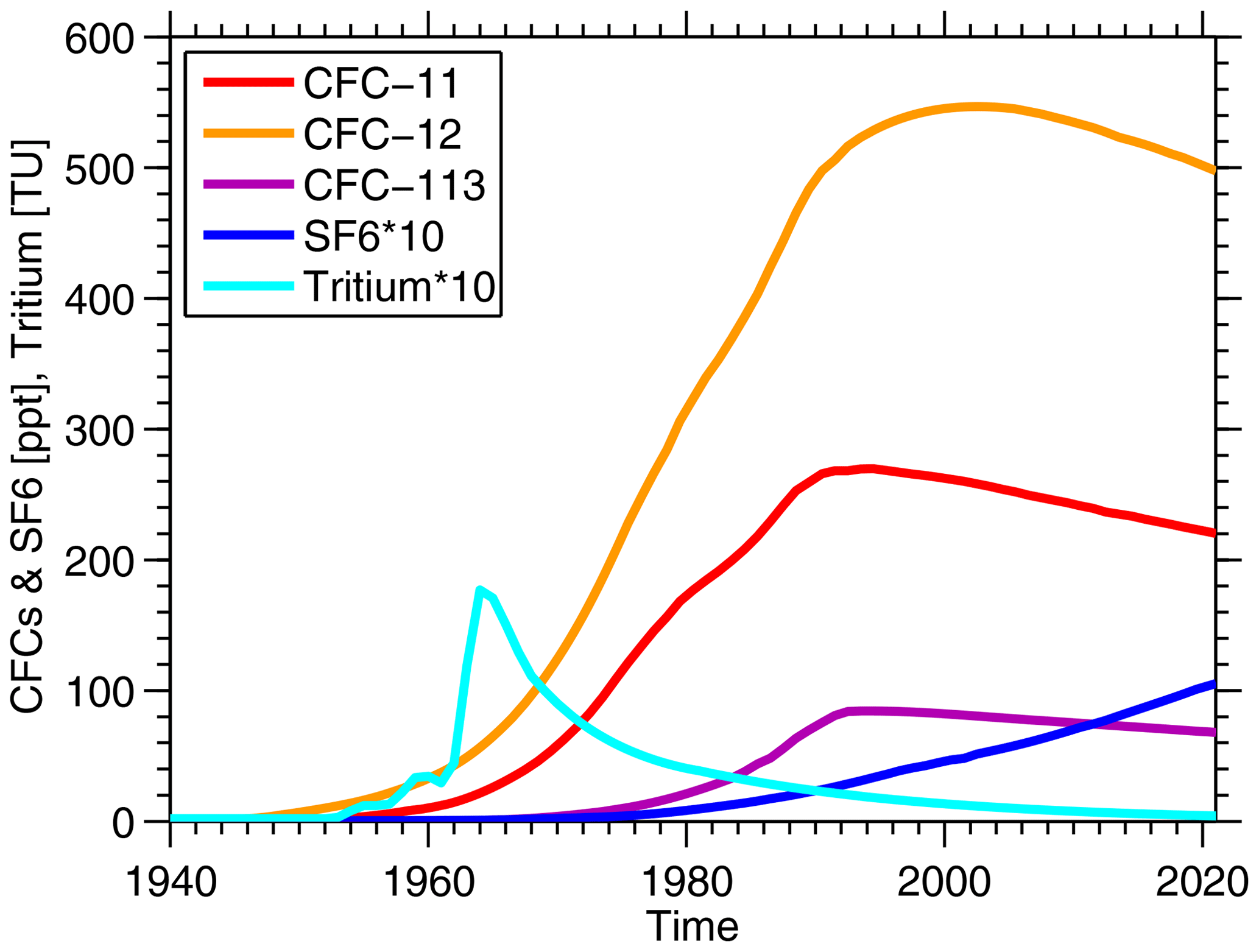
Figure C1 Time history of CFC-11, CFC-12, SF₆ and tritium for the Northern Hemisphere (the North Atlantic for tritium).

Appendix D: Variation in TTD parameters

The effect of the choice of the TTD parameters on the shape of the TTD and the inferred C_ant concentration is illustrated in Fig. D1 and Table C1. We assume a CFC-12 concentration of 0.4 pmol kg⁻¹ observed in 2010, a CFC saturation of 0.85, a potential temperature of θ = 3 °C and a salinity of S = 34.9. C_ant is calculated for the reference year 2010 and an alkalinity of 2308 µmol kg⁻¹ (the value derived from Lee et al., 2006, for the North Atlantic). The maximum of the TTD occurs at younger ages for $\mathrm{\Delta }/\mathrm{\Gamma }=\mathrm{2}$ compared to the case with $\mathrm{\Delta }/\mathrm{\Gamma }=\mathrm{1}$. This is a fairly common behavior; i.e., increasing the $\mathrm{\Delta }/\mathrm{\Gamma }$ ratio leads to a younger age of the mode of the TTD. Reducing the fraction of young water leads to an even younger mode, although in this case the $\mathrm{\Delta }/\mathrm{\Gamma }$ ratio is always chosen as 1. The younger the mode of the possible TTDs derived from a given CFC-12 concentration, the smaller the inferred C_ant concentration (see Table D1).

The TTD 𝒢_young for the young water in Fig. D1 only represents half of the water, as the fraction f in this example equals 0.5. To illustrate what the complete TTD might look like, we assume an old TTD 𝒢_old with Γ =500 years and Δ =250 years. The sum of 𝒢_young and 𝒢_old is shown as the dashed line in Fig. D1. This choice of the parameters for 𝒢_old is arbitrary, but it fulfills the condition that the inferred C_ant concentration is small (< 0.5 µmol kg⁻¹ in this case) and thus might be neglected. The sum of 𝒢_young and 𝒢_old only has one clear maximum. The mode of 𝒢_old is much less pronounced than that of 𝒢_young, so the complete TTD has a kind of saddle point around the mode of 𝒢_old (250 years in the example in Fig. D1).

Table D1 TTD parameters derived for a CFC-12 concentration of 0.4 pmol kg⁻¹ in 2010, assuming a CFC saturation of 0.85, a potential temperature of θ = 3 °C and a salinity of S = 34.9. C_ant is calculated for the reference year 2010 and an alkalinity of 2308 µmol kg⁻¹ (the value derived from Lee et al., 2006, for the North Atlantic). Also given is the fraction of water older than 200 years.

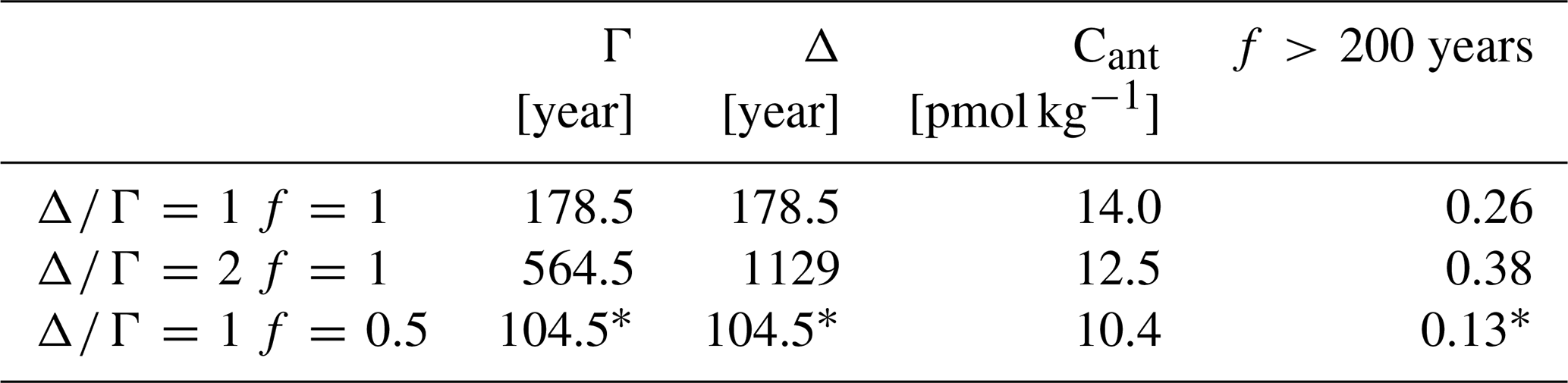
^* Values are for the young TTD component only.

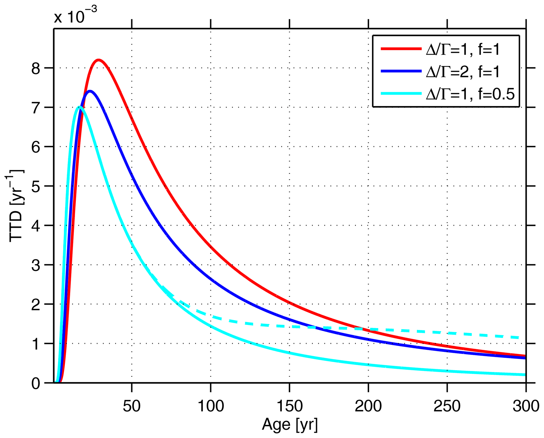
Figure D1 TTDs derived from an observed CFC-12 concentration of 0.4 pmol kg⁻¹ in 2010, a CFC saturation of 0.85, a potential temperature of θ = 3 °C and a salinity of S = 34.9. Shown are TTDs for f = 1, $\mathrm{\Delta }/\mathrm{\Gamma }=\mathrm{1}$ and $\mathrm{\Delta }/\mathrm{\Gamma }=\mathrm{2}$, as well as TTDs for f = 0.5 and $\mathrm{\Delta }/\mathrm{\Gamma }=\mathrm{1}$. For the latter case, an assumed old TTD with Γ =500 years and Δ =250 years is also added (dashed cyan line).

Appendix E: Relative C_ant change (Δ_tC_ant) between 1990 and 2020

Figure E1 shows the relative increase in the C_ant column inventory for the periods of 1990–2000, 2000–2010 and 2010–2020. In contrast, in Fig. 12 from the main text the absolute values of the C_ant increase are shown. From the rising atmospheric CO₂ concentration and a steady-state ocean, a decadal increase in the C_ant inventory of about 19 % would be expected.

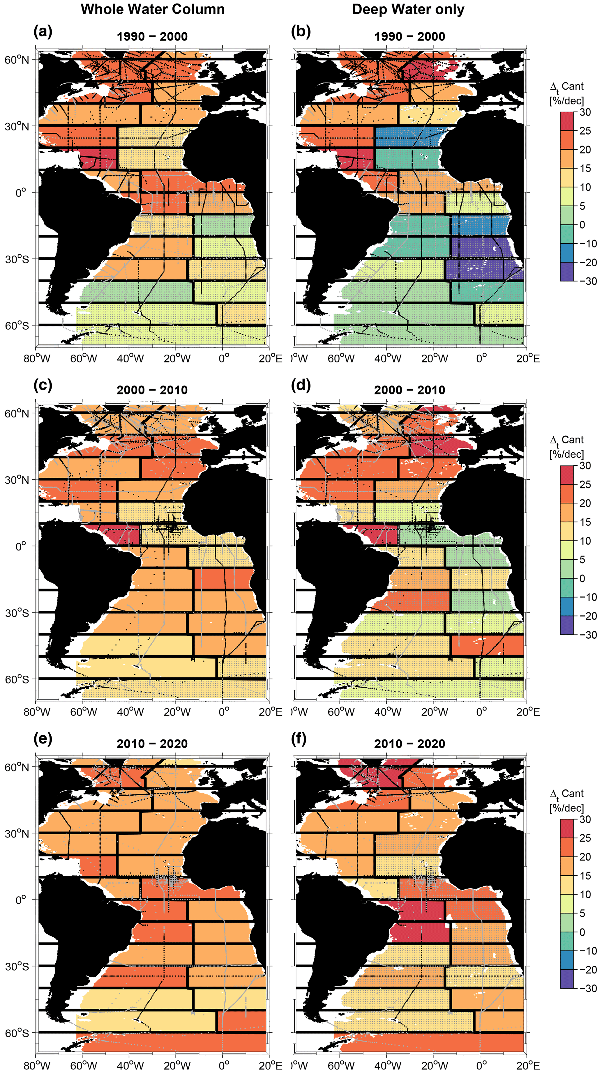
Figure E1 (a, c, e) Whole water column, (b, d, f) only deep and bottom water masses. (a, b) 1990–2000, (c, d) 2000–2010, (e, f) 2010–2020. Only areas with a water depth larger than 200 m are considered. Station locations for the first period (1982–1994 in a, b; 1995–2005 in c, d; and 2006–2013 in e, f) are marked in light grey, and those for the second period (1995–2005 in a, b; 2006–2013 in c, d; and 2014–2021 in e, f) are marked in black. Regions with differences smaller than the error range are stippled. Note the uneven spacing between contour intervals.