CO₂ emissions of drained coastal peatlands in the Netherlands and potential emission reduction by water infiltration systems

Worldwide, the drainage of peatlands has turned these systems from CO₂ sinks into sources. In the Netherlands, where ∼7 % of the land surface consists of peatlands, drained peat soils contribute >90 % and ∼3 % to the country's soil-derived and total CO₂ emissions, respectively. Hence, the Dutch National Climate Agreement has set targets to cut these emissions. One potential mitigation measure is the application of subsurface water infiltration systems (WISs) consisting of subsurface pipes connected to ditchwater. WISs aim to raise the water table depth (WTD) in dry periods to limit peat oxidation while maintaining current land-use practices. Here, we used automated transparent chambers in 12 peat pasture plots across the Netherlands to measure CO₂ fluxes at high frequency and assess (1) the relationship between WTD and CO₂ emissions for Dutch peatlands and (2) the effectiveness of WISs in mitigating emissions. Net ecosystem carbon balances (NECBs) (up to 4 years per site, 2020–2023) averaged 3.77 and 2.66 $\mathrm{t}{\mathrm{CO}}_{\mathrm{2}}\text{-}\mathrm{C}{\mathrm{ha}}^{-\mathrm{1}}{\mathrm{yr}}^{-\mathrm{1}}$ for control and WIS sites, respectively. The magnitude of NECBs and the slope of the WTD–NECB relationship fall within the range of observations of earlier studies in Europe, though they were notably lower than those based on campaign-wise, closed-chamber measurements. The relationship between annual exposed carbon (C; defined as the total amount of carbon within the soil above the average annual WTD) and NECB explained more variance than the WTD–NECB relationship. The magnitude of the NECB represented 1.0 % of the annual exposed C on average, with a maximum of 2.4 %. We found strong evidence for a reducing effect of WISs on CO₂ emissions, reducing emissions by 2.1 (95 % confidence interval 1.2–3.0) $\mathrm{t}{\mathrm{CO}}_{\mathrm{2}}\text{-}\mathrm{C}{\mathrm{ha}}^{-\mathrm{1}}{\mathrm{yr}}^{-\mathrm{1}}$, and no evidence for an effect of WISs on the WTD–NECB and annual exposed carbon–NECB relationships. This means that relationships between either WTD or exposed carbon and NECB can be used to estimate the emission reduction for a given WIS-induced increase in WTD or exposed carbon. High year-to-year variation in NECBs calls for multi-year measurements and sufficient representative measurement years per site as demonstrated in this study with 35 site-year observations.

1 Introduction

Peatlands only cover 3 % of the Earth's surface, yet they store 30 % of the global soil carbon (C) and thereby function as an important global C sink (Friedlingstein et al., 2022; Leifeld and Menichetti, 2018; Yu et al., 2010). Peatlands consist of non- or partly decomposed plant material and are typically formed under wet and anoxic conditions when the supply of dead plant material exceeds decomposition. However, many peatlands worldwide have been drained and claimed for human purposes – mainly agriculture and forestry – during the last centuries (Kaat and Joosten, 2009; UNEP, 2022). Drainage immediately halts peat formation and increases soil aeration, which in turn accelerates aerobic microbial peat decomposition. This effectively reverses a peatland's function as a CO₂ sink by emitting large amounts of CO₂ – sequestered over thousands of years – back into the atmosphere (Erkens et al., 2016; Evans et al., 2021; Tiemeyer et al., 2020). Worldwide, drained peatlands are responsible for 2 %–5 % of total anthropogenic greenhouse gas (GHG) emissions (Bonn et al., 2016; Humpenöder et al., 2020; Leifeld and Menichetti, 2018). Given the high CO₂ emissions from drained peatlands, reducing these emissions would be a prerequisite to reach targets set by the Paris Climate Agreement to keep global warming below 1.5–2.0 °C (Leifeld and Menichetti, 2018). Hence, prompt measures are needed to limit CO₂ emissions from peatlands.

The Netherlands arguably has the longest history of intensive drainage and exploitation of peat soils in the world (Erkens et al., 2016). Currently, about 290 000 ha (ca. 7 % of the Dutch land surface) consists of peat soils of which ca. 77 % is used for agriculture, primarily as pastures for dairy farming (Arets et al., 2021). Due to deltaic and coastal conditions, 17 % and 36 % of coastal peatlands in the Netherlands are covered by a thick (40–80 cm) and thin (<40 cm) clay cover, respectively (Jansen et al., 2009). Cultivated, drained peat soils in the Netherlands emit an estimated 4 Mt CO₂ yr⁻¹ (Arets et al., 2021), constituting ca. 3 % of the country's total CO₂ emissions (CBS, 2023). The Dutch Climate Agreement (Ministry of Economic Affairs and Climate Policy, 2019) targets a reduction of 1 $\mathrm{Mt}{\mathrm{CO}}_{\mathrm{2}}\text{-}\mathrm{eq}.{\mathrm{yr}}^{-\mathrm{1}}$ from drained peat areas by 2030 and a 95 % reduction in emissions by 2050 relative to 1990. Hence, there is an urgency to explore, test, and apply emission mitigation measures in drained peatlands.

Most proposed mitigation measures rely on limiting or reversing the drainage of peatlands, thereby (temporarily) decreasing water table depths (WTDs). A shallow WTD decreases the extent of the unsaturated zone, limiting the maximum depth of oxygen intrusion into the soil (Boonman et al., 2024b), thereby mitigating aerobic decomposition and CO₂ emissions. There are indeed several studies that show a clear relationship between WTD and CO₂ emissions, although they differ in the type of relation and magnitude of emissions. Some studies suggest a linear relationship between WTD and CO₂ emissions (e.g. Couwenberg et al., 2011; Evans et al., 2021). Others, such as Tiemeyer et al. (2020) and Koch et al. (2023), found a relationship that fitted best with a sigmoid function, whereby changes in WTD at depths beyond 30 cm hardly affect CO₂ emissions (meaning that raising the WTD is only useful at shallow depths). Of these studies, CO₂ emissions reported in Tiemeyer et al. (2020) were the highest, being a factor 1.7 and 7.4 higher for a WTD between 0.2–0.4 m compared to Couwenberg et al. (2011) and Evans et al. (2021), respectively.

Several land management strategies are available to decrease peatland drainage, peat decomposition, and the corresponding CO₂ emissions. Options include complete peatland rewetting for nature restoration (Nugent et al., 2019) or paludiculture (Abel and Kallweit, 2022; Wichtmann and Joosten, 2007), which are effective in limiting peat oxidation (Tanneberger et al., 2022; Buzacott et al., 2024; van den Berg et al., 2024), but this also means moving away from conventional agricultural land use. To maintain conventional agricultural use, alternative options include raising ditchwater levels or applying (sub)surface water infiltration systems (WISs; e.g. Boonman et al., 2022; van den Akker et al., 2008; Weideveld et al., 2021) to reduce peat oxidation, albeit to a lesser extent than complete rewetting. In the Dutch coastal peatland areas, WISs consist of regularly spaced subsurface drains (commonly 4–6 m drain spacing), which are connected to ditches or to a managed reservoir. These systems allow a more homogeneous WTD within a field, thereby decreasing the extent of the unsaturated zone in warm and dry summers. As spacing between ditches in these areas is commonly large (30–100 m), raising ditchwater levels would be less efficient than WISs in reducing the unsaturated zone thickness further away from the ditch, as the hydraulic conductivity of degraded peat soils is mostly low (Jansen et al., 2007; Kechavarzi et al., 2007; Liu et al., 2016). By reducing the unsaturated zone, the application of WISs is expected to reduce aerobic peat decomposition and associated CO₂ emissions while allowing conventional agricultural activities to continue. However, the effectiveness of WISs in terms of CO₂ emission reduction varies, since some studies found evidence for a decrease in yearly CO₂ emissions from WISs (Boonman et al., 2022, 2024a; Offermanns et al., 2023; van den Akker et al., 2008), while other studies found insufficient evidence (Weideveld et al., 2021) or even found evidence for an increase in CO₂ emissions (Tiemeyer et al., 2024). Differences in reported effectiveness may be caused by differences in soil properties or hydrological boundary conditions (ditchwater level, seepage, summer drought, or wet conditions), among others.

This study presents the measurement results from a novel CO₂ emission monitoring network for Dutch coastal peatlands under intensive agricultural use using automated transparent chambers. The aim of this network is twofold: (1) to establish a relationship between WTD and annual CO₂ emissions, and its uncertainty, for this specific type of peatland and (2) to determine the effectivity of WISs as a measure to reduce CO₂ emissions from these peatlands. We derived annual net ecosystem carbon balance (NECB) estimates for six locations for up to 4 years (2020–2023) from high-frequency CO₂ flux measurements with automated transparent chambers. We then evaluated the relations between WTD and NECB estimates and determined the WIS effectiveness in terms of annual NECB differences in relation to effective changes in WTD.

2 Methods

Six locations distributed over the coastal peat areas in the Netherlands were selected (Sect. 2.1, Fig. 1, Table 1) for this study. The locations were instrumented with automated transparent chambers (Sect. 2.2) and environmental sensors (Sect. 2.3). Plots were harvested and fertilised (Sect. 2.4), resulting in several C input and export terms that are considered in the NECB estimates (Sect. 2.5).

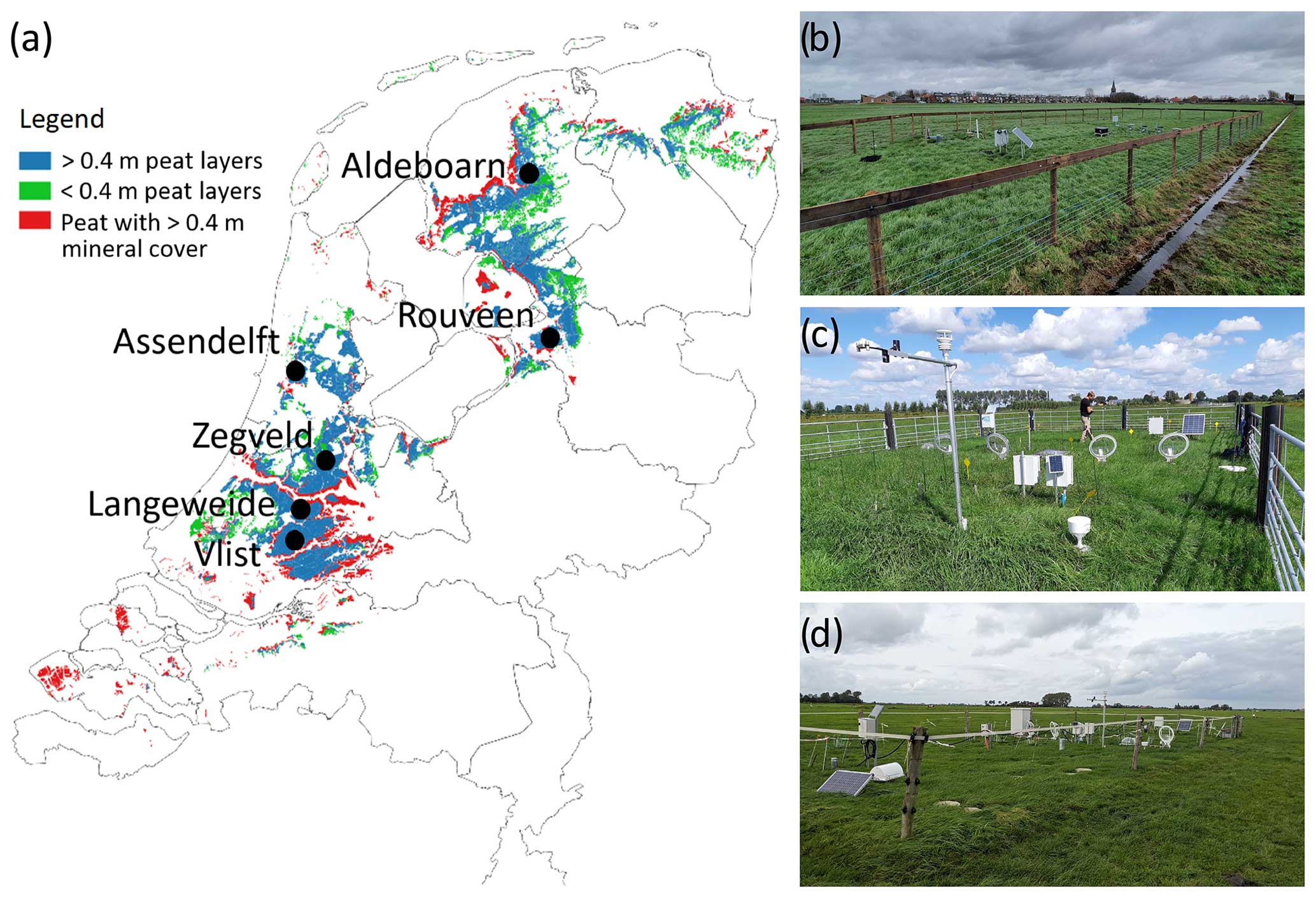
Figure 1 Site locations and presence of coastal peatlands in the Netherlands (a). Photo impressions of Assendelft (b), Zegveld (c), and Aldeboarn (d).

Table 1 Overview of some characteristics of the measurement sites addressed in this paper, distinguishing the control (CON) and treatment (passive or active water infiltration; WIS) plots per location. Both the listed WTD and the ditchwater table (WT) apply to summer values. Peat thickness applies to the total Holocene peat layer thickness, and clay thickness applies to the thickness of the clay(ey) layer on top of the peat. All units are in m.

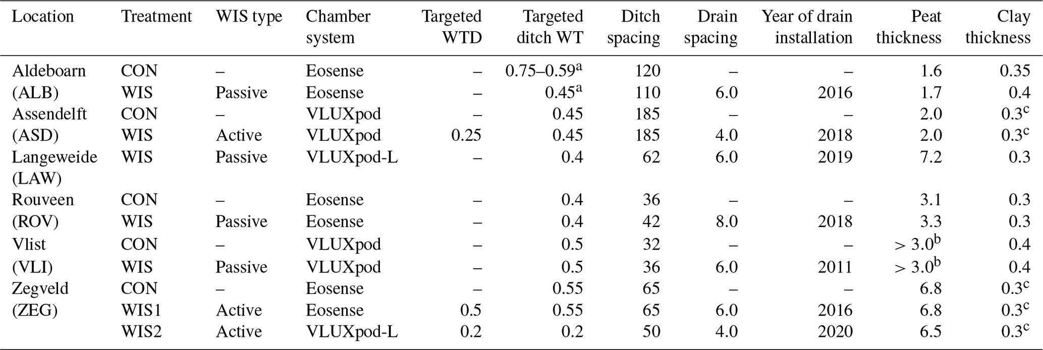
^a CON: change in ditch WT from an ∼ constant 0.75 m in 2021 to a fluctuating (range: 0.37–0.88 m) level thereafter. The range presented in the table represents the range in the annual average ditchwater table. WIS: fluctuating ditchwater level controlled by the farmer until March 2022, fixed at 0.45 m thereafter. ^b Alternating layers of clay and peat. The total peat thickness exceeds 3 m. ^c The top 0.3 m of the profile consists of peaty clay or clayey peat.

2.1 Study sites and study setup

Six locations were selected where water infiltration systems (WISs; sometimes also called submerged drains) had (recently) been installed. These locations are distributed over the coastal peatlands (peatlands with surface level elevation below 1 m above mean sea level) in the Netherlands taking into account the following selection criteria: (1) the peat layer (>80 % organic matter) thickness exceeds 1 m, (2) the peat layer is covered by less than 0.5 m of clay, and (3) locations are used as intensively managed grasslands which are mowed and/or grazed (Fig. 1). Five locations had both a control (CON; without WIS) and a treatment field (with WIS); see Table 1. One location (LAW) only consisted of a treatment field, and, in one location (ZEG), we measured two different treatment fields which were compared with one control.

The control fields were drained via ditches and, in some fields, furrows. Ditches always carried water and had (more or less) fixed summer and winter water levels, except for one location (ALB WIS; see Table 1). The treatment fields were drained via the same routes as the control fields, with the addition of a WIS. The WIS primarily increases water infiltration during dry (summer) periods but also promotes drainage during wet (mostly winter) periods. Various configurations of WIS were used: subsurface drain tubes may be connected directly to the ditch below the water level (passive water infiltration system) or to a managed reservoir controlled by a pump (active water infiltration system). The latter system aims to actively maintain a target water table depth (WTD) in the field. The type of system per location is indicated in Table 1.

Measurement plots of the various locations in this study were set up in a similar fashion. A measurement plot of approximately 200 m² was fenced off. In the treatment plots, automated transparent flux chambers and subsurface sensors (Sect. 3.3) were installed in 3- or 4-fold (1) above or in proximity to a WIS drain, (2) at a quarter distance between two WIS drains, and (3) midway between two WIS drains (Fig. S1 in the Supplement). In the control plot, the same spatial distribution of measuring devices was used, although not related to the presence of a drain tube.

The soil C profiles across the study sites (Hefting et al., 2023) are visualised in Fig. 2. There is considerable variation in the average soil C content above the average WTD measured over the study period. In ALB this average soil C content was lowest (71–73 kg C m⁻³), while it was highest in ZEG (122–148 kg C m⁻³).

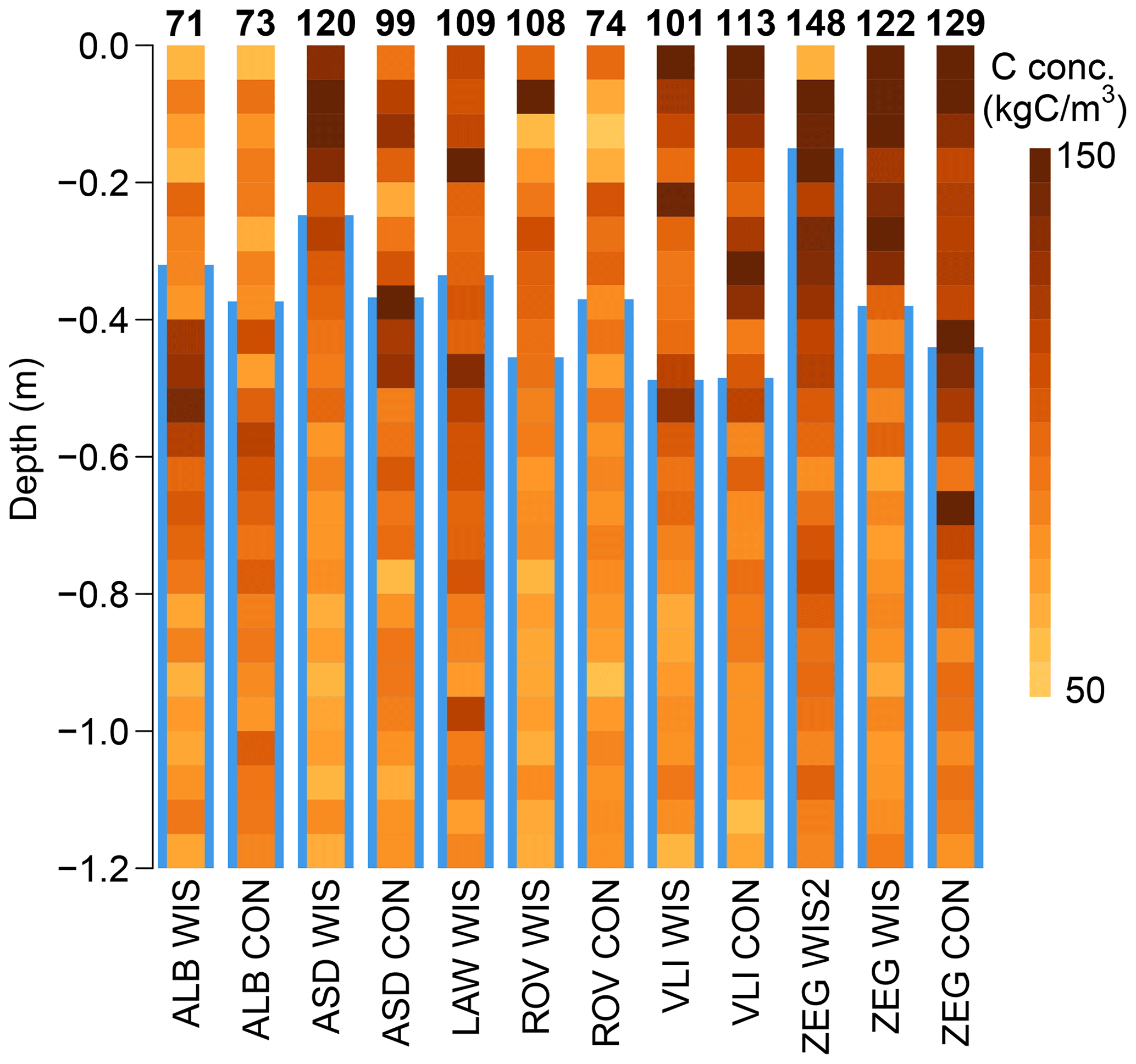
Figure 2 Soil carbon profiles of all study sites (Hefting et al., 2023). The average water table depth (WTD) per plot is visualised by the blue bars in the background of each carbon profile, and the average carbon density (kg C m⁻³) above the WTD is given above each profile.

2.2 Automated transparent chamber CO₂ flux measurements

2.2.1 Chamber types

Fluxes of CO₂ between the soil–vegetation system and the atmosphere were estimated from CO₂ concentration changes in closed chambers. For this, we used three types of automated transparent chamber systems (Table 1, Fig. 3). These automated chambers allow continuous, day, and night measurements of CO₂ concentrations at a high frequency. In all systems we used an infrared gas analyser (LI-850, LI-COR) to measure concentrations of CO₂ and H₂O that were logged by a Campbell CR1000x data logger once every 2 s.

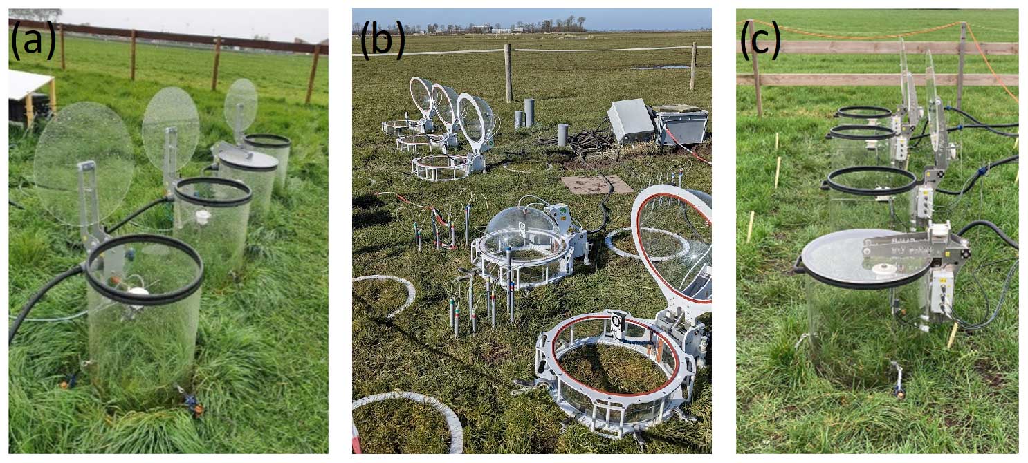
Figure 3 Transparent chamber systems: (a) VLUXpod, (b) Eosense eosAC-LT, and (c) VLUXpod-L chambers.

In ALB, ROV, and ZEG (CON and WIS1), CO₂ fluxes on each plot were estimated using three eosAC-LT chambers (Eosense) connected to a multiplexer (eosMX; Eosense). Each chamber had a total height of 41.2 cm and a volume of 72 L and consisted of a transparent base (height: 15 cm; diameter: 52 cm) and a transparent dome-shaped lid, which was opened and closed by a linear actuator closing in 15 to 30 s. Chambers were placed on permanent serrated soil collars (15 cm deep). These collars offset the original chamber height by 0.5–6 cm, depending on soil swelling and shrinking; collar heights for ALB and ROV were measured during site maintenance to adjust the volume used for flux calculations (see below). For ZEG CON and WIS, an average offset of 1 cm was used, as no consistent measurements were available. All three chambers were connected to the multiplexer, which was used to control the chambers and route gas to the analyser. Recirculation of gas was achieved using the LI-850's built-in pump (0.75 L min⁻¹) and PTFE tubing to and from the chamber (8–10 m, one way). Every 30 min, chambers were measured sequentially with a 2.5 min closure time and a 15–45 s flushing period in between.

In ASD and VLI, a custom-built chamber system (referred to as “VLUXpod” chambers) was used. Each system consisted of four transparent cylindrical chambers (volume ∼62 L) with a base height of 50 cm, a diameter of 40 cm, and a transparent flat lid that was pneumatically controlled, which opened and closed within 2 s. In contrast to the Eosense chambers, no permanent soil collar was used, but a custom-built tool was used to make 1–5 cm deep incisions into the soil to seal the chamber walls to the soil surface. The chamber height relative to the soil surface was measured when chambers were relocated. A multiplexer with an external pump (2.5 L min⁻¹; KNF NMP830KNDC-B 12V) was used to control the system and recirculate gas (8–10 m of polyurethane tubing, one way), from which gas was sampled by the analyser. Every 15 min, chambers were measured sequentially using a 3 min closure time and 15–45 s flushing in between.

A third system (“VLUXpod-L chambers”) was used in ZEG WIS2 and LAW, which consisted of a similar setup to the aforementioned VLUXpod chambers. The main difference between the two was a larger diameter of 50 cm rather than 40 cm and the presence of a higher-flow gas circulation pump (5 L min⁻¹; KNF NMP830KPDC-B HP 12V).

2.2.2 Chamber operation

Chambers were moved and cleaned approximately every 2 weeks to limit lasting effects of an altered microclimate inside the chambers on the vegetation and soil. The chambers were rotated over three rows (with three or four chambers per row, depending on the system) such that any chamber location was occupied approximately 33 % of the time. Grass heights were measured upon every chamber movement in all chamber rows. Chamber systems (including analysers) were removed from the field for maintenance and analyser calibration once every year. All chamber systems were equipped with a low-flow fan to achieve a well-mixed headspace (Christiansen et al., 2011; Rochette and Hutchinson, 2005).

2.2.3 Flux estimation

The CO₂ flux, hereafter named net ecosystem exchange (NEE; $\mathrm{\mu }\mathrm{mol}{\mathrm{CO}}_{\mathrm{2}}{\mathrm{m}}^{-\mathrm{2}}{\mathrm{s}}^{-\mathrm{1}}$), was calculated as

$$\begin{array}{}\text{(1)}& \text{NEE}={\displaystyle \frac{VP\left(\mathrm{1}-\frac{W}{\mathrm{1000}}\right)f}{RS(T+\mathrm{273.15})}},\end{array}$$

where V (m³) is the chamber volume, corrected for changes in collar or chamber height over time; P (Pa) is the air pressure measured by each location's weather station; W is the water vapour mole fraction as measured by the ${\mathrm{CO}}_{\mathrm{2}}/{\mathrm{H}}_{\mathrm{2}}\mathrm{O}$ analyser (mmol mol⁻¹); f is the rate of change in water-corrected CO₂ mole fraction ($\mathrm{\mu }\mathrm{mol}{\mathrm{mol}}^{-\mathrm{1}}{\mathrm{s}}^{-\mathrm{1}}$) inside the closed chamber; R is the ideal gas constant (8.314 $\mathrm{Pa}{\mathrm{m}}^{\mathrm{3}}{\mathrm{K}}^{-\mathrm{1}}{\mathrm{mol}}^{-\mathrm{1}}$); S (m²) is the soil surface area; and T (°C) is the air temperature measured inside the chamber (VLUXpod chambers) or measured at 2 m height by the weather station (Eosense chambers). To determine f, we applied linear regression and a variety of regression periods. For each individual chamber system, regression periods were chosen such that only the linear portion of the concentration change was selected (Maier et al., 2022). This was required to limit the effects of chamber closure that resulted in nonlinear concentration changes, such as (1) headspace CO₂ depletion and glass-clouding during the daytime and (2) spikes in CO₂ concentration that often occur immediately after chamber closure during nights with atmospheric stratification (Koskinen et al., 2014). As such, daytime regression lengths were restricted to a maximum of 30 to 60 s, starting just after the deadband (i.e. start of concentration change in response to chamber closure) to capture the initial slope, whereas nighttime regression periods could be longer (up to 160 s) and started up to 100 s after chamber closure.

Data were left out from the flux calculation when analyser cell pressures or temperatures were outside of the calibrated operating range, when gas concentrations were erroneous (e.g. due to IR source failure), and in cases of other types of system malfunctioning (e.g. non-functional fans or non-functioning chamber lids) or system maintenance. In some cases, a small correction to the measured concentrations was applied based on drift in analyser calibration. A visual inspection of the data together with an automated quality control was applied to filter out other poor linear regression fits. The automated filtering procedure was based on a combination of regression fit characteristics, such as r², RMSE, and actual flux slope. Thresholds for filtering deviated per chamber system and period considered.

2.2.4 Flux partitioning and gap-filling

For further processing, we aggregated NEE fluxes by taking the mean of the measured fluxes of all chambers in a specific field over a half-hour period. Due to data quality control and system maintenance and malfunctioning, gaps were present in the aggregated flux data with extents ranging from half an hour to multiple weeks. We identified a gap as having no flux estimates from any of the chambers in the specific field during the half-hour period. An overview of the data availability per site is given in Fig. 4. To fill these gaps, as required to obtain an annual NECB estimate, we separated the 30 min averaged net ecosystem exchange (NEE) flux into gross primary production (GPP) and ecosystem respiration (R_eco).

$$\begin{array}{}\text{(2)}& \text{NEE}=R_{\text{eco}}-\text{GPP}\end{array}$$

We model daytime R_eco based on nighttime R_eco, compensated for temperature differences only. Although it is common practice to model daytime R_eco based on nighttime R_eco estimates, we acknowledge that it can lead to biased estimates due to divergent temperature dependencies of day- and nighttime R_eco resulting from processes such as inhibited leaf respiration in light (Järveoja et al., 2020; Keenan et al., 2019).

$$\begin{array}{}\text{(3)}& R_{\text{eco}}=R_{\text{ref}}\cdot e^{E_{\mathrm{0}}\cdot \left(\frac{\mathrm{1}}{(T_{\text{ref}}-T_o)}-\frac{\mathrm{1}}{(T-T_{\mathrm{0}})}\right)},\end{array}$$

where R_ref ($\mathrm{\mu }\mathrm{mol}{\mathrm{CO}}_{\mathrm{2}}{\mathrm{m}}^{-\mathrm{2}}{\mathrm{s}}^{-\mathrm{1}}$) is the reference respiration rate, E₀ (K) is the long-term ecosystem sensitivity coefficient to temperature, T_ref (K) is the reference temperature for which the reference respiration was determined, T₀ (K) is the base temperature (set at 227.13 K; Lloyd and Taylor, 1994), and T (K) is the observed soil temperature at 5 cm depth. To obtain a site-specific estimate of the long-term ecosystem sensitivity coefficient, Eq. (3) was applied to all measured daily averaged nighttime data for the whole time series at one location, with a reference temperature of 10 °C.

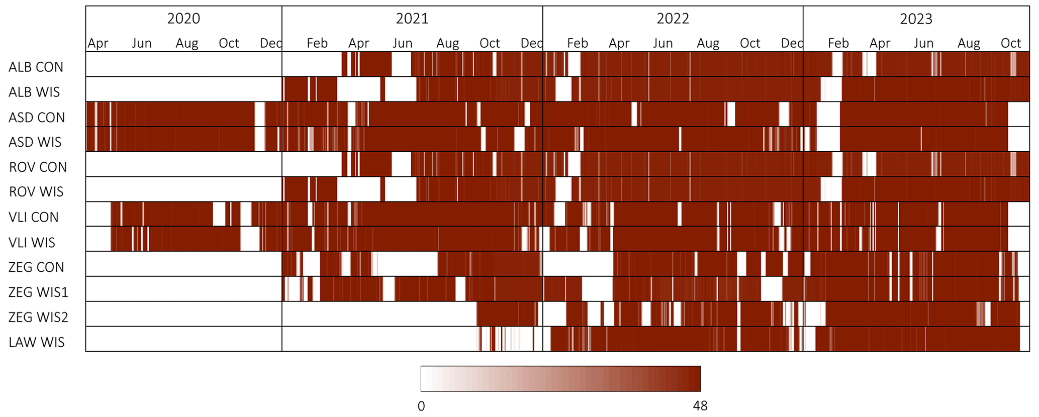
Figure 4 Overview of CO₂ flux data availability on all sites. Red in different shades indicates data availability, where the darkest red refers to 48 half-hour data points per day and white refers to no data available. Sites were set up at different moments; therefore, the starting dates of the flux measurements differ per site. Note that the periods depicted here as calendar years are not necessarily used to calculate annual net ecosystem carbon balances (Table S1).

Daytime fluxes were partitioned based on the standard procedure as described by Falge et al. (2001), Oestmann et al. (2022), Tiemeyer et al. (2016), and Veenendaal et al. (2007). Given the site-specific value of E₀, daytime R_eco was modelled on a half-hourly basis using Eq. (3), with R_ref and T_ref given by the daily averaged nighttime respiration rate and soil temperature at 5 cm depth, respectively, and with T as the measured soil temperature at 5 cm depth during the half-hour intervals. With the daytime calculated R_eco, an estimate of GPP was obtained using measured NEE and Eq. (2). GPP can be described by a rectangular hyperbolic light response curve (LRC) based on Michaelis–Menten kinetics (Oestmann et al., 2022), given by

$$\begin{array}{}\text{(4)}& \text{GPP}={\displaystyle \frac{{\text{GPP}}_{\mathrm{2000}}\times \mathit{\alpha }\times \text{PAR}}{{\text{GPP}}_{\mathrm{2000}}+\mathit{\alpha }\times \text{PAR}-\frac{{\text{GPP}}_{\mathrm{2000}}}{\mathrm{2000}\mathrm{\mu }\mathrm{mol}{\mathrm{m}}^{-\mathrm{2}}{\mathrm{s}}^{-\mathrm{1}}}\times \text{PAR}}},\end{array}$$

where GPP₂₀₀₀ ($\mathrm{\mu }\mathrm{mol}{\mathrm{CO}}_{\mathrm{2}}{\mathrm{m}}^{-\mathrm{2}}{\mathrm{s}}^{-\mathrm{1}}$) is the rate of C fixation at a PAR value of 2000, α ($\mathrm{\mu }\mathrm{mol}{\mathrm{CO}}_{\mathrm{2}}{\mathrm{m}}^{-\mathrm{2}}{\mathrm{s}}^{-\mathrm{1}}/\mathrm{\mu }\mathrm{mol}\mathrm{PAR}{\mathrm{m}}^{-\mathrm{2}}{\mathrm{s}}^{-\mathrm{1}})$ is the light-use efficiency (the initial slope of the LRC), and PAR is the measured photosynthetically active radiation ($\mathrm{\mu }\mathrm{mol}{\mathrm{m}}^{-\mathrm{2}}{\mathrm{s}}^{-\mathrm{1}}$). As we determined GPP by partitioning, the (time-variant) parameters (GPP₂₀₀₀ and α) could be obtained on a daily basis by fitting the LRC on the partitioned GPP.

In cases of data gaps (Fig. 4) in the half-hourly aggregated data, R_eco and GPP were gap-filled separately where daily obtained parameters from Eqs. (3) and (4) (smoothened with a moving average of 5 d) were linearly interpolated. In the event of harvest, the moving average was cut off before and after harvest, and LRC parameters were set to a minimum after harvest, to subsequently increase linearly to the obtained parameters 5 d after harvest. When a gap occurred over a harvest period, the parameters were taken up to 3 d before or after (in the case of R_eco) harvest. If gaps were larger than this period, parameters were obtained from similar harvest moments from that site.

2.3 Environmental variables

On each of the plots, we measured soil temperature (Drill and Drop probes, Sentek Technologies) and phreatic groundwater and surface water levels (ElliTrack-D, Leiderdorp Instruments). The 30 min averaged soil temperatures were logged at 10 cm depth intervals from 5 to 115 cm depth. Phreatic groundwater levels were measured in monitoring wells, which were founded in deeper sand layers below the peat to assure a constant reference level. They were logged once every hour. Groundwater levels relative to the actual field height (i.e. WTD; Fig. S2) were calculated from surface movement measurements obtained from an extensometer (Van Asselen et al., 2020) combined with spirit levelling (four times a year) to account for spatial differences in field height. Each of these variables was measured in at least three locations within each plot. For the WIS plot, these locations were next to the drain at a quarter distance between drains and midway between two drains. Meteorological measurements included air temperature and pressure (at a 30 min logging interval), as measured in each location's control plot at 2.0 m height using a MaxiMet GMX500 (Gill instruments Limited). Precipitation was measured using an ARG314 tipping bucket rain gauge (Environmental Measurements Limited). PAR was measured at 1.8 m height (1 min logging interval) using an SKR 1840D (Skye Instruments).

We determined the annual and summer mean WTD per plot (WTD_a and WTD_s, respectively) by averaging the three measurement locations per plot, where annual refers to the total period of the 1-year budget (Sect. 2.5) and summer refers to the months of April to September. The soil C profiles (Fig. 2) were used to determine the annual and summer mean soil C exposure per plot (Cexp_a and Cexp_s, respectively), taking the cumulative soil C amounts from soil surface to annual and summer mean WTD.

2.4 Harvest and fertilisation

Plots were typically fertilised five times per year and mown five to nine times per year, aiming for at least once every 4 weeks during the growing season. Fertilisation was done with known quantities of mineral NPK (first two events) or N (remaining events) fertiliser for all sites, except for ALB, where manure was used, as it is an organic farm. All sites used the same amounts and composition of mineral fertiliser (∼250 kg N, 108 kg P₂O₅, and 195 $\mathrm{kg}{\mathrm{K}}_{\mathrm{2}}\mathrm{O}{\mathrm{ha}}^{-\mathrm{1}}{\mathrm{yr}}^{-\mathrm{1}}$). Applied manure and grass samples were weighed and analysed for C content.

To determine the C exported via grass harvests, grass yield was quantified for each chamber individually by weighing wet and dry (oven-dried for 48 h at 70 °C) biomass. For ALB and ROV, the average harvest per chamber per mowing event was determined as the average of grass yields collected from the different positions upon which the chamber is rotated, weighted by the amount of time that the chamber spent on each position. For other sites the grass was sampled only from the current chamber position. For ASD and VLI, differences in grass height in different chamber positions proved to be of minor importance. From the grass samples collected during each mowing event, the average and standard deviation (SD) of the C export of the different chambers per harvesting event were calculated.

For ALB and ROV, dried biomass samples were chopped using a cutting mill (SM 200, Retsch). Then, a homogenised subsample was ground using a mixer mill (MM 400, Retsch). Grounded biomass (4–5 mg) was weighed into tin capsules and analysed for C content using an NA 1500 elemental analyser (Carlo Erba). For all other locations, samples were sent to a commercial laboratory (Eurofins, Wageningen, the Netherlands), where they were thoroughly mixed and split into subsamples. The dried biomass was ground <1 mm, and C was determined using near-infrared spectroscopy (NIRS) performed on a Q-Interline machine. The standard Eurofins Agro calibration curves for common Dutch grasslands (the most common species grown is Lolium perenne) were used, which are based on calibrations against wet chemistry (Harris et al., 2018).

2.5 Carbon budgets

The C budget of each site is given as the net ecosystem carbon balance (NECB) over a period of 1 year:

$$\begin{array}{}\text{(5)}& \text{NECB}=\text{NEE}+{\mathrm{C}}_{\text{export}}-{\mathrm{C}}_{\text{input}},\end{array}$$

with all terms given in $\mathrm{t}\mathrm{C}{\mathrm{ha}}^{-\mathrm{1}}{\mathrm{yr}}^{-\mathrm{1}}$ (Chapin et al., 2006). Positive C fluxes and budgets indicate a loss of C from the soil–vegetation system to the atmosphere. Note that the C budget in Eq. (5) does not account for C changes via runoff; lateral subsurface flow; and the emission of CH₄, CO, and volatile organic C. Inorganic carbon is not added to the experimental fields and is also not widely present in the soil profile. Inorganic carbon is present in the soil water phase as dissolved CO₂ and ${{\mathrm{HCO}}_{\mathrm{3}}}^{-}$, mostly originating from peat decomposition. For the NECB calculation, we assume that changes in inorganic carbon in the soil profile including the water phase on a yearly basis (1 January–1 January) are small compared to the GPP and R_eco fluxes and mostly fall within the uncertainty bounds of the overall fluxes. The input term in Eq. (5) consists of applied manure and is only relevant in ALB, as other locations were fertilised with mineral fertiliser. The export term in Eq. (5) consists of harvested biomass, which is assumed to be released as CO₂ elsewhere during the year and is factored in as loss from the system.

As a measure of spatial heterogeneity, we also gap-filled half-hourly fluxes of each chamber individually and obtained the SD between the daily mean NEE fluxes in each chamber (SD_NEE). Furthermore, if any day in the half-hourly chamber-averaged flux dataset consisted of less than 30 half-hour flux measurements, we added an extra gap-fill SD term (SD_gap), depending on the length of the gap. The term was determined by creating artificial gaps of 1, 5, 15, and 30 d and by comparing differences between measured data and gap-filled data. A linear relation was found between SD and gap size, which we extrapolated to obtain an estimate of the SD for any gap in the data. The SD of the fertilisation C import term (for ALB only) was estimated at 50 % of the total C import. The SD of the resulting NECB was then obtained with Eq. (6) as

$$\begin{array}{}\text{(6)}& {\displaystyle }{\text{SD}}_{\text{NECB}}=\sqrt{\left\{\begin{array}{c}\sum {\text{SD}}_{\text{NEE}}^{\mathrm{2}}+\sum {\text{SD}}_{\text{gap}}^{\mathrm{2}}\\ +\sum {\text{SD}}_{{\mathrm{C}}_{\text{export}}}^{\mathrm{2}}+\sum {\text{SD}}_{{\mathrm{C}}_{\text{import}}}^{\mathrm{2}}\end{array}\right\}},\end{array}$$

where each term is the sum of the occurrences in each year.

2.6 Statistics

All calculations and statistics were carried out in R (R Core Team, 2023). Pearson's correlation coefficient (r) was computed using the cor function of the “stats” package. To establish relationships between NECB and potential predictors (i.e. WTD and Cexp), we used simple linear models (LMs) using the lm function of the “stats” package. To statistically compare the NECBs of the CON and WIS treatments, we used linear mixed-effects models (LMMs) using the lmer function of the “lme4” package (Bates et al., 2015b) with treatment as a fixed effect. The effect of treatment on the relationship of NECB with potential predictors (i.e. WTD and Cexp) was tested using the interaction of treatment with the predictor of interest as a fixed effect. To deal with the non-independence in the dataset (i.e. having multiple NECBs per location and per year), we treated the measurement year nested in location as a random effect on the model's intercept for all LMMs mentioned above. In cases where the fitted LMM was evaluated to be (near) singular (i.e. NECB∼WTD_a) due to the variance estimate of random effect, “year”, being near zero, we ran the model with only location as a random effect, thereby following recommendations in Barr et al. (2013) and Bates et al. (2015a). To statistically compare the WTD–NECB relationship based on our data and those of other drained peatlands, we used NECB as the response variable, the interaction of WTD with the data source as a fixed effect, and location as a random effect on the model intercept. We used type-III ANOVAs (function ANOVA) to test the significance of the fixed effects of our various LMMs, with degrees of freedom and p-values calculated using the Kenward–Roger approximation (Kenward and Roger, 1997) integrated in the “pbkrtest” and “lmerTest” packages (Halekoh and Højsgaard, 2014; Kuznetsova et al., 2017). Model assumptions of linearity, homoscedasticity, and normality of residuals were checked using residual plots, histograms and Q–Q plots of residuals, and the Shapiro–Wilk test (function Shapiro.test of package “stats”). When communicating our statistical results, we use the language of evidence as suggested by Muff et al. (2022).

3 Results and discussion

3.1 Chamber CO₂ flux estimates and carbon balances

We collected 12 485 daily CO₂ flux estimates, comprised of roughly 517 000 half-hourly means, based on ∼3.1 million observed fluxes. We observed clear variability in the CO₂ fluxes for all locations and plots on temporal scales ranging from minutes to seasons (Fig. 5). The daily CO₂ fluxes ranged from −179 (net uptake) to 163 kg (net emission) of ${\mathrm{CO}}_{\mathrm{2}}\text{-}\mathrm{C}{\mathrm{ha}}^{-\mathrm{1}}{\mathrm{d}}^{-\mathrm{1}}$. The median daily CO₂ flux across all plots for the full study period was −5.1 $\mathrm{kg}{\mathrm{CO}}_{\mathrm{2}}\text{-}\mathrm{C}{\mathrm{ha}}^{-\mathrm{1}}{\mathrm{d}}^{-\mathrm{1}}$. The highest daily net uptake rates were mostly confined to spring, while the highest daily net emission rates generally occurred during summer. The aggregated half-hourly CO₂ flux data availability for the individual annual budget periods and sites considered was 83 % on average. We omitted the budgets of ALB WIS, ROV WIS, and ZEG CON in 2021 from further analysis due to the low data availability and the large consecutive periods of missing data during the growing season (Fig. 4, Table S1 in the Supplement) for which extensive gap-filling was required.

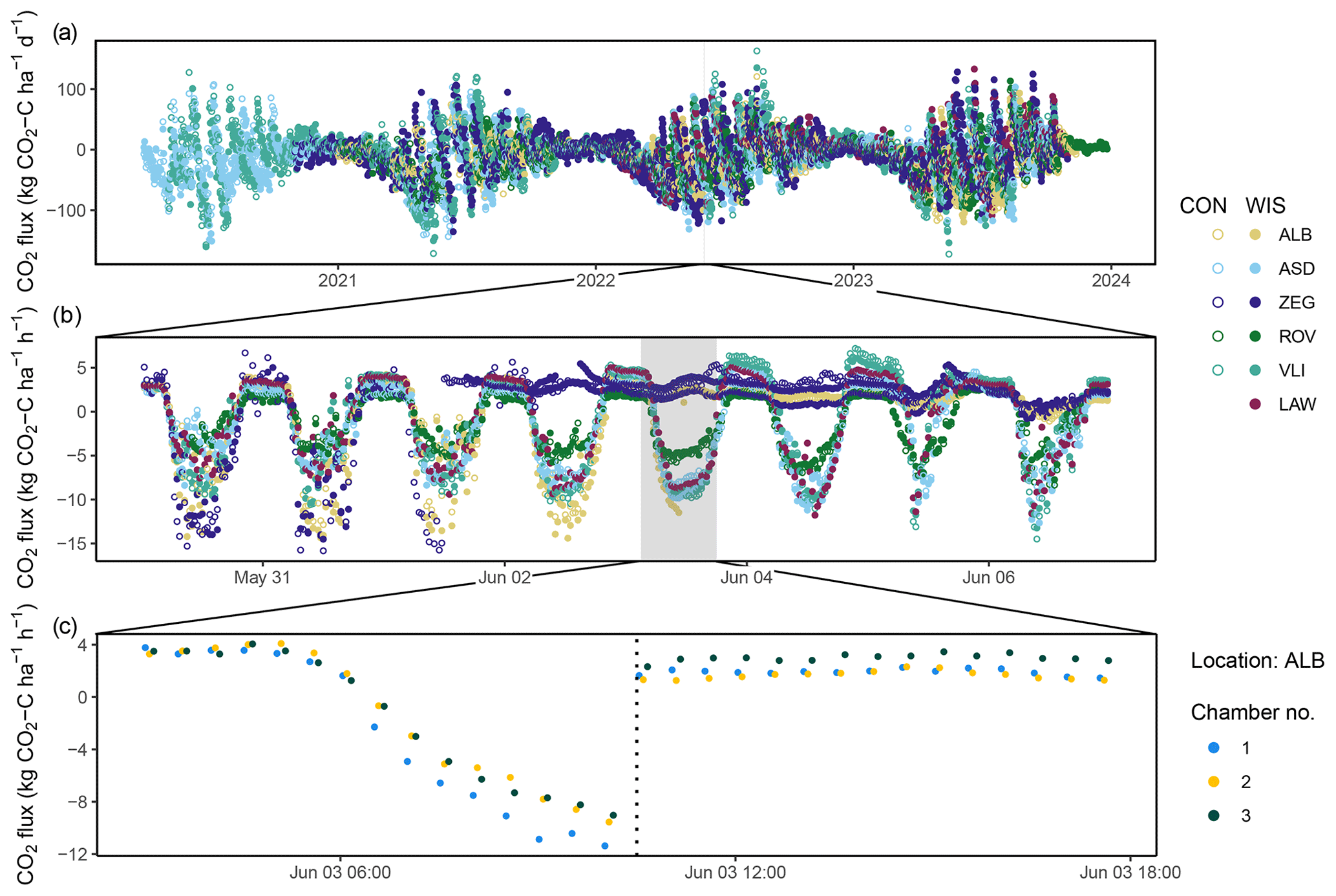
Figure 5 Temporal variability in CO₂ fluxes observed at different timescales: (a) daily means of each location and treatment (i.e. control (CON) and water infiltration system (WIS)) for the full study period, (b) half-hourly means for each location and plot for the shaded period in panel (a), and (c) CO₂ fluxes for each individual chamber of ALB CON for the shaded period in panel (b). The dotted line in panel (c) denotes a mowing event. Note that ZEG WIS has two time series included due to measurements at two different WIS sites.

An overview of the annual C balances is presented in Fig. 6, distinguishing between NEE, harvest export, and manure import. Harvest was especially high in 2020 and 2021. For most locations and years, it provides the largest C flux of the terms considered in this figure, with 6.4 $\mathrm{t}\mathrm{C}{\mathrm{ha}}^{-\mathrm{1}}{\mathrm{yr}}^{-\mathrm{1}}$ on average. This term is in the higher range of what was found on German peatland sites with Lolium perenne (1.3–6.4 $\mathrm{t}\mathrm{C}{\mathrm{ha}}^{-\mathrm{1}}{\mathrm{yr}}^{-\mathrm{1}}$; Tiemeyer et al., 2020). Higher yields in our locations are likely due to high fertilisation application and the frequent harvest events during growing season (∼5–7 vs. 1–5 cuts in Tiemeyer et al., 2020). In ZEG WIS2, harvests are generally lower than in the WIS1 and CON plot of ZEG, likely owing to oxygen stress in the root zone (Bartholomeus et al., 2008), given the shallow WTD_s (0.18, 0.49, and 0.64 m in WIS2, WIS1, and CON, respectively). The same applies for ASD WIS, where harvests are generally lower than for ASD CON (with an average WTD_s of 0.30 and 0.55 m in WIS and CON, respectively). NEE terms are mostly negative and show quite a lot of year-to-year variation (Fig. 6). NEE was highest (i.e. close to zero) in LAW, VLI, and ROV and was lowest (i.e. strongest net uptake) in ALB and ASD.

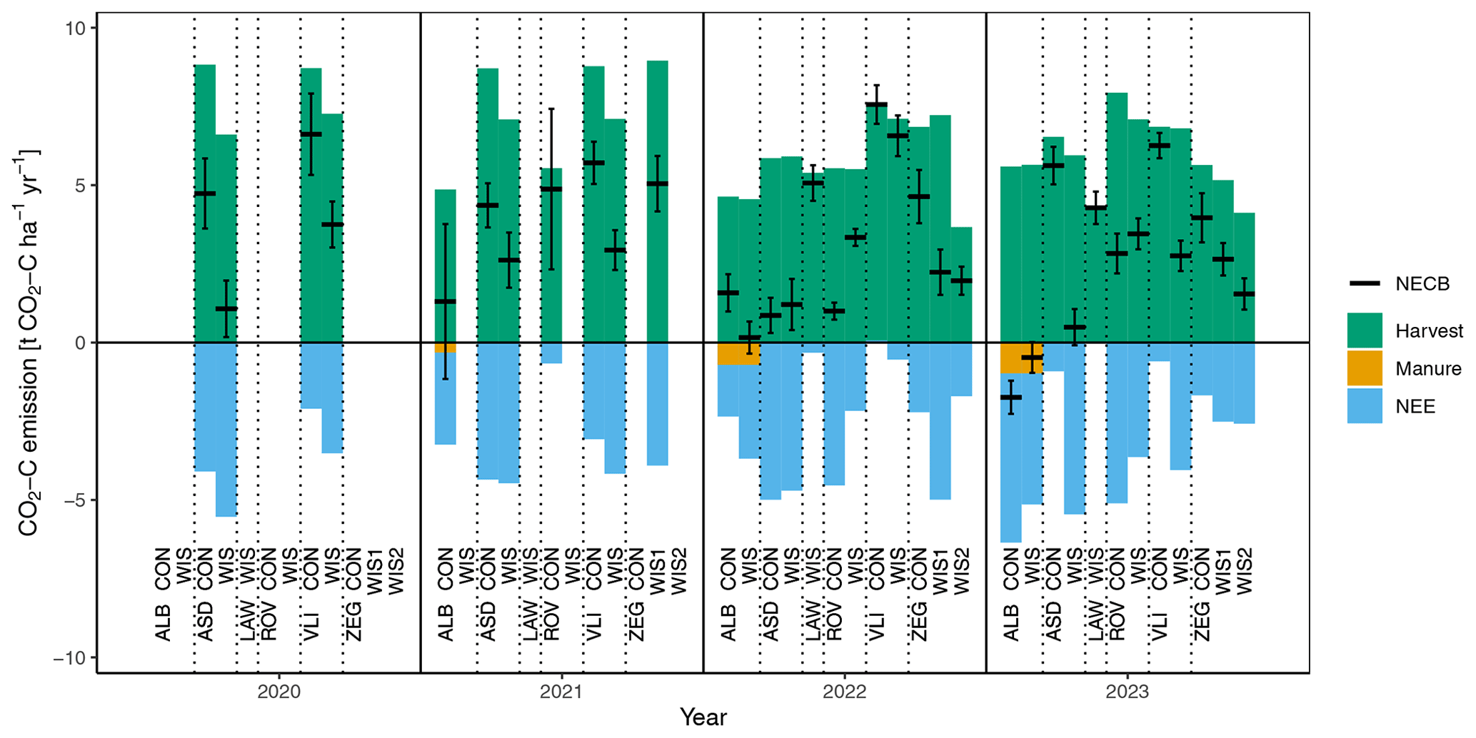
Figure 6 Annual CO₂ emission terms (with uptake being negative) as net ecosystem exchange (NEE), harvest, and manure (only in ALB) of the plots over the years 2020–2023. The horizontal black lines indicate the net ecosystem carbon balance (NECB), including their standard deviations (indicated by whiskers). Specific values are also provided in Table S1.

The estimated terms GPP and R_eco, being the two constituents of NEE, are substantially larger than the terms displayed in Fig. 6, with values ranging from −18 to −29 $\mathrm{t}\mathrm{C}{\mathrm{ha}}^{-\mathrm{1}}{\mathrm{yr}}^{-\mathrm{1}}$ for GPP and 14 to 25 $\mathrm{t}\mathrm{C}{\mathrm{ha}}^{-\mathrm{1}}{\mathrm{yr}}^{-\mathrm{1}}$ for R_eco (Table S1). The high harvest export term was also reflected in the GPP: in almost all cases, the uptake of C by plants (GPP) exceeded the respiration (R_eco), leading to negative NEEs (on average −3.0 $\mathrm{t}\mathrm{C}{\mathrm{ha}}^{-\mathrm{1}}{\mathrm{yr}}^{-\mathrm{1}}$). On the contrary, in German peatland sites with Lolium perenne, the average NEE was +8.1 $\mathrm{t}\mathrm{C}{\mathrm{ha}}^{-\mathrm{1}}{\mathrm{yr}}^{-\mathrm{1}}$ (Tiemeyer et al., 2020), while the average NEE of boreal and temperate peatlands used as grassland in Evans et al. (2021) was +1.3 $\mathrm{t}\mathrm{C}{\mathrm{ha}}^{-\mathrm{1}}{\mathrm{yr}}^{-\mathrm{1}}$.

NECB, being the result of NEE, harvest export, and manure import, shows a similar year-to-year variability to NEE and harvest export, and it averaged 3.17 $\mathrm{t}\mathrm{C}{\mathrm{ha}}^{-\mathrm{1}}{\mathrm{yr}}^{-\mathrm{1}}$ across all site years. In almost all cases the sum of NEE and harvest export led to positive NECBs. Only in ALB did we estimate NECBs to be ∼0 in 2022 (WIS) and negative in 2023 (both WIS and CON). The substantial negative NECB estimates in 2023 are caused by a high negative NEE. This site, being the only site in the north of the Netherlands (Fig. 1), is quite different from the other sites in this study due to its 0.4 m thick clay cover, the lowest soil C content in the upper soil layer of all sites (Fig. 2), deviating peat composition, deviating land-use history (having experienced more deeply drained conditions), and ongoing manure application. Though these factors are likely to affect the magnitude of the NECBs, they cannot explain why the NECBs are negative, especially since positive NECBs (8.1–17.9 $\mathrm{t}\mathrm{C}{\mathrm{ha}}^{-\mathrm{1}}{\mathrm{yr}}^{-\mathrm{1}}$) were found at the same site using campaign-wise measurements with manual chambers in 2017 and 2018 (Weideveld et al., 2021). In addition, NECBs of 2.8 and 6.4 $\mathrm{t}\mathrm{C}{\mathrm{ha}}^{-\mathrm{1}}{\mathrm{yr}}^{-\mathrm{1}}$ were estimated for the ALB WIS and CON field, respectively, using eddy covariance measurements (period October 2021–October 2022; unpublished data). We currently do not have an explanation for the widely varying results and negative NECBs for this particular site; however, these could be related to unquantified C fluxes, such as lateral transport of C via groundwater, C export via geese or mice, or a change in C storage in the root zone. Also, a dependency on the methods used to obtain the flux estimates (e.g. measurement technique and method of data processing) may be responsible for the varying results.

Another noticeable annual C budget is found in the CON plot of ASD in 2022. In this year, we obtained an exceptionally low NECB in the CON plot compared to the other year budgets on that plot. In this specific year, chambers of the CON plot were moved to a different location within the plot, as the vegetation within the original chamber locations in this year was no longer representative for the vegetation within the plot. However, as there is no evidence of a high degree of spatial heterogeneity in e.g. soil parameters within the plot, we cannot appoint any concrete reasons why moving the chambers could have resulted in such a low NECB in the CON plot for this year.

3.2 Relationships between NECB and controlling variables

In Fig. 7 and Table 2 we show how the annual C budgets relate to WTD_s (Fig. 7a, r²=0.19) and WTD_a (Fig. 7b, r²=0.15). Because of warmer temperatures and deeper groundwater levels during summer, we expected the NECBs to relate substantially better to WTD_s than to WTD_a, as proposed by Boonman et al. (2022). Our results, however, do not convincingly support this hypothesis and only show a slightly higher explained variance for the WTD_s. The similar performance of the two models is likely explained by the strong correlation between WTD_a and WTD_s (Pearson's r=0.88).

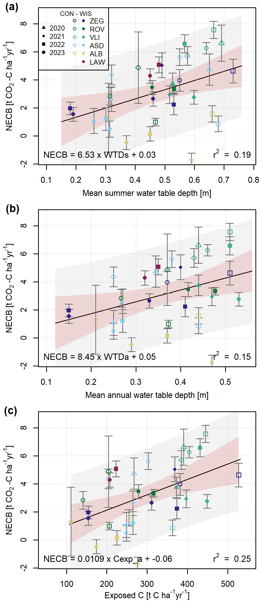
Figure 7 Mean summer (a) and annual (b) water table depth and (c) annual exposed carbon with estimated net ecosystem carbon balances (NECBs) presented in Table S1. NECB standard deviations are included as error bars. Linear models (Table 2) are fitted on the data and plotted with the 90 % intercept prediction intervals (grey) and 95 % confidence intervals from the linear model estimation (red).

Table 2 Linear model fits for NECB and explanatory variables related to water table depth (WTD) and exposed soil carbon (Cexp) presented in Fig. 7 and Table S1.

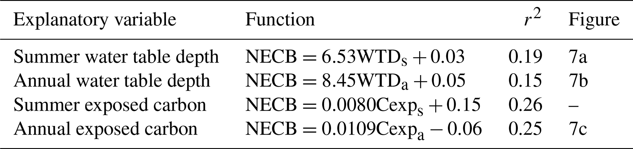
The relation between NECB and total exposed C within the soil profile above the average annual WTD (Cexp_a) was stronger (Fig. 7c, r²=0.25) than the relation with WTD_a. The same is true for the relation between NECB and summer exposed C (Cexp_s) as compared to the relation with WTD_s (r² of 0.26 and 0.19, respectively). Since relationships with Cexp explained more variance than those with WTD, we propose to use Cexp rather than WTD_a as a predictor for NECB. The use of Cexp will be particularly important in the coastal zone and deltaic peatlands because, in these environments, flooding-derived clastic layers commonly cover the peat layers (Koster et al., 2018).

The low and even negative NECBs from ALB, as mentioned in the previous section, are generally much lower than predicted by the linear regression and are positioned just inside or even outside the prediction intervals (Fig. 7a and b). However, when expressed against exposed soil C rather than WTD (Fig. 7c), these data points better approach predicted values, owing to the relatively low C stock in the upper part of these soils (Fig. 2). While Tiemeyer et al. (2016) showed that NECB relates to aerated soil N stock rather than C stock, our data suggest that exposed C does relate to NECB. We found that the magnitude of the NECB represented 1.1 % of the annual exposed C on average, with a maximum of 2.4 %.

While simple linear regression is widely applied to fit empirical relations to explain measured NECBs (e.g. Couwenberg et al., 2011; Evans et al., 2021), we tested several alternative linear models for the relation between WTD_a and NECB (Table S2) and inspected the variation in slope and intercept. We included robust linear regression where the weights of outliers are decreased, Deming regression that accounts for observation error estimates, and a linear mixed-effects model (LMM) that explicitly models the non-independence in the data (Harrison et al., 2018). The best estimate of the slope of the different linear models ranged from 4.81 (LMM) to 14.35 (Deming model), with the best estimate of the intercept varying from −2.31 (Deming model) to 1.37 (LMM) (Table S2). The best estimate of the slopes of each of these alternative linear regressions was well within the 95 % confidence intervals of the slope estimate of the simple linear regression. The same was true for the intercept that was statistically indistinguishable from zero for all models (Table S2).

3.3 Effectiveness of WIS

The average NECB over all the years for the individual plots as a function of their average WTD_a and Cexp_a is shown in Fig. 8a and b, respectively. There is a trend of lower NECBs in the WIS plots compared to the control plots. One notable exception to this trend is ROV. Here, the NECB of the WIS plot exceeds that of the CON plot for the 2 available years. This location is situated in an area with upward seepage of groundwater, which results in the unintended situation where the WIS mostly drains rather than infiltrates water. This, in turn, causes a deeper WTD (and higher Cexp) for the WIS plot compared to the CON plot. In this case, a higher NECB in the WIS plot is in line with the expectation based on the relations presented in Table 2.

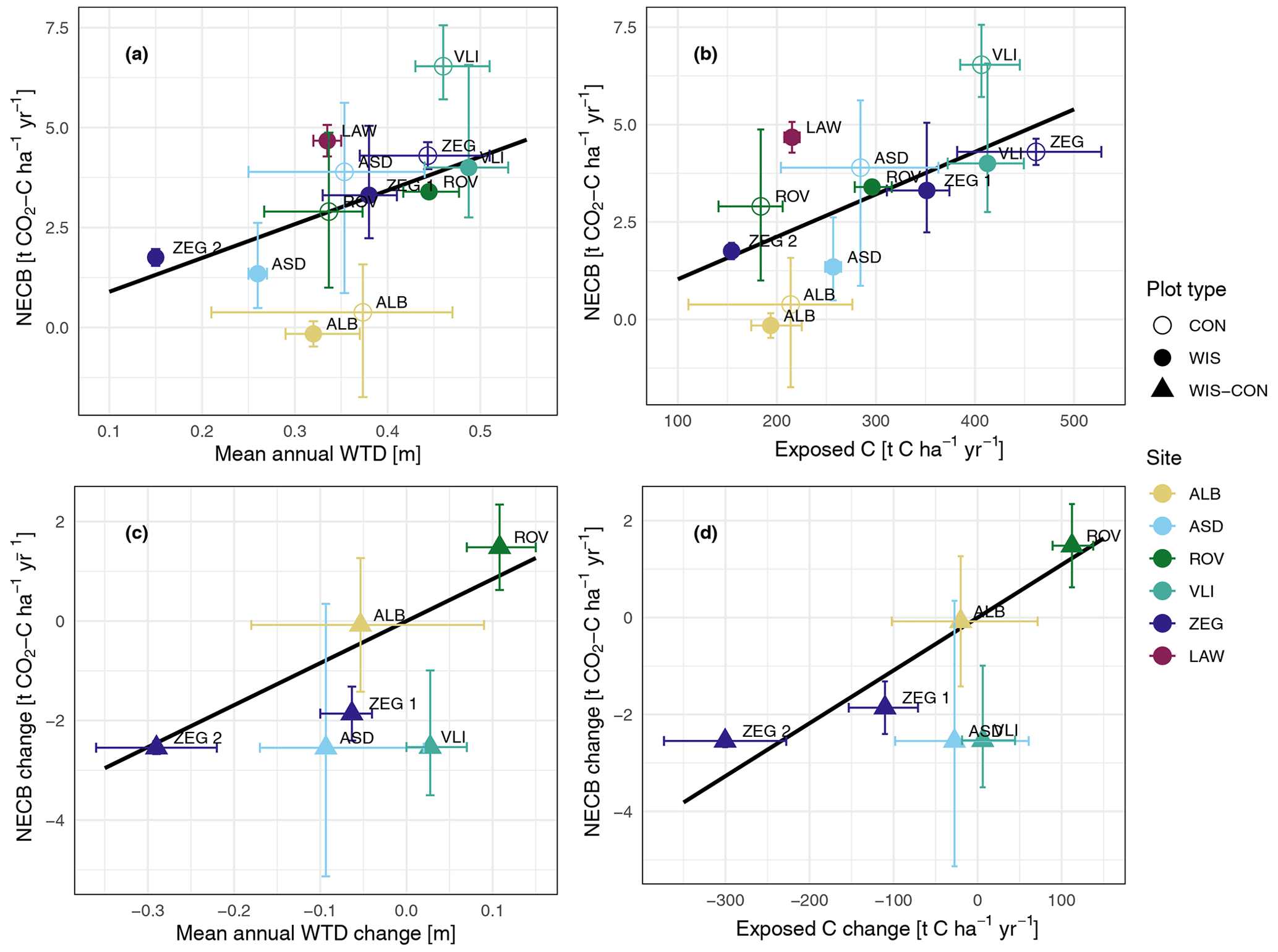
Figure 8 Averaged annual net ecosystem carbon balance (NECB) per plot as a function of (a) averaged annual water table depth (WTD), (b) averaged annual soil C exposure, (c) averaged annual difference in NECB between WIS and CON (as WIS−CON) sites per location as a function of averaged annual difference in WTD, and (d) averaged annual difference in soil C exposure. Solid black lines are the linear model fits of Fig. 7. Whiskers indicate minimum and maximum annual values per location or plot.

The question of whether WIS is effective in reducing CO₂ emissions can be addressed in various ways. For example, one may treat WIS and CON as discrete variables. When including the previously mentioned location with upward seepage (ROV), excluding the location that did not have both WIS and CON sites (LAW), and excluding location years when either the WIS or the CON site did not have data available (i.e. ALB, ROV, and ZEG in 2021), the average NECB on WIS sites was 2.26 (16 site years) $\mathrm{t}{\mathrm{CO}}_{\mathrm{2}}\text{-}\mathrm{C}{\mathrm{ha}}^{-\mathrm{1}}{\mathrm{yr}}^{-\mathrm{1}}$ and was 3.86 (14 site years) $\mathrm{t}{\mathrm{CO}}_{\mathrm{2}}\text{-}\mathrm{C}{\mathrm{ha}}^{-\mathrm{1}}{\mathrm{yr}}^{-\mathrm{1}}$ on CON sites. Excluding ROV, the average WIS and CON NECBs were 2.10 (14 site years) and 4.19 (12 site years) $\mathrm{t}{\mathrm{CO}}_{\mathrm{2}}\text{-}\mathrm{C}{\mathrm{ha}}^{-\mathrm{1}}{\mathrm{yr}}^{-\mathrm{1}}$, respectively. We find very strong evidence of a reducing effect of WIS on the NECB (LMM: $F_{\mathrm{1},\mathrm{13}}=\mathrm{20.82}$, $P=\mathrm{5.26}\times {\mathrm{10}}^{-\mathrm{4}}$) when excluding ROV and strong evidence of an effect of WIS ($F_{\mathrm{1},\mathrm{15}}=\mathrm{9.50}$, P=0.0075) when including ROV.

As the primary reason for implementation of WIS is to achieve a shallower WTDs, we can also treat WIS as a continuous variable by considering the effect of WIS on the WTD or Cexp. To do so, we regard the difference in WTD or Cexp between the WIS and CON plots as the explanatory variable and the difference in NECB between the two plots as the effect. This way, situations where WIS results in a deeper WTD (i.e. contrary to the intended water infiltration effect, as observed in ROV) can also be assessed: as based on the relations in Table 2, we expect a higher NECB when WIS deepens the WTD. This comparison is visualised in Fig. 8c and d for WTD_a and Cexp_a, respectively. The linear relation displayed in these graphs is the linear relation given in Table 2 and used in Fig. 8a and b and seems to fit adequately to the points in the graph. A simple linear regression through these data points does not yield a significantly different slope.

To further strengthen this argument, we found no evidence for an effect of WIS on the relationship between NECB and WTD (LMM: $F_{\mathrm{1},\mathrm{24}}=\mathrm{0.79}$ and P=0.38 for WTD_a and $F_{\mathrm{1},\mathrm{23}}=\mathrm{0.52}$ and P=0.48 for WTD_s), as was suggested by Boonman et al. (2022), or between NECB and Cexp (LMM: $F_{\mathrm{1},\mathrm{20}}=\mathrm{0.12}$ and P=0.74 for Cexp_a and $F_{\mathrm{1},\mathrm{19}}=\mathrm{0.11}$ and P=0.74 for Cexp_s). This implies that the potential impact that WIS may have on environmental factors, such as soil temperature, nutrient status, electron acceptor availability, or oxygen and dissolved organic C availability, falls within the uncertainty of year-to-year and site-to-site variability when using only WTD or exposed C as explanatory variables. This suggests that the linear model fits presented in Table 2 (within the available data ranges) can estimate the reduction in NECB due to a change in WTD or exposed C owing to the implementation of WIS. Therefore, we conclude that if WIS is able to raise the groundwater table substantially, it has a reducing effect on the NECB, based on the paired-site comparisons and statistics of fitted WTD–NECB models with slopes exceeding zero in all cases (Table S2).

Previous research showed that WIS resulted in neglectable effects on the NECB (Weideveld et al., 2021), a higher NECB (Tiemeyer et al., 2024), or a mild (Offermanns et al., 2023) to strong (Boonman et al., 2022, 2024a; van den Akker et al., 2008) reduction in NECB. Here we show that NECB changes in WIS sites are dependent on the actual changes in WTD or exposed C and that, in some cases, a neglectable or even slightly adverse effect of WIS (as in ALB and ROV, respectively) can be expected if changes in WTD or exposed C are minimal or opposite to the aim of WIS.

Apart from WIS, which typically leads to a moderate WTD increase, more drastic WTD regulation could be implemented to allow paludiculture (Geurts et al., 2019; Martens et al., 2023) or restoration to a full peat-growing ecosystem (Nugent et al., 2019) as more effective measures to limit (or even reverse) peat loss (Girkin et al., 2023). When applying these alternative measures, the relation between WTD and NECB that we defined might not be directly applicable due to vegetation differences and a WTD range. Also, at a shallower WTD, other GHGs such as CH₄ and N₂O might offset reductions in CO₂ emissions (Evans et al., 2021; Tiemeyer et al., 2020). Furthermore, a broader perspective on measures (other than GHG emissions) will be necessary, since WIS can only reduce peat oxidation to a certain extent, while overall net-zero emission is aimed for in 2050. Although we recognise that WIS is an attractive measure to reduce CO₂ emissions without changing land use, we emphasise the need for inclusion of other aspects with respect to the future of managed peatlands. Measures to counteract peat oxidation should always be evaluated from different disciplines and stakeholder perspectives.

3.4 NECB estimations and water table depth relationships in perspective

The NECB and WTD observations presented in this study are similar to those of other empirical relations of Evans et al. (2021), Boonman et al. (2022), and Fritz et al. (2017) (Fig. 9, Table S3). However, several other studies found considerably higher emissions from drained peatlands for WTD_a deeper than 0.2 m below the surface (Couwenberg et al., 2011; Koch et al., 2023; Tiemeyer et al., 2020). The IPCC emission factors for CO₂ emissions from drained organic soils are also higher: the IPCC Wetlands Supplement (IPCC, 2014) contains separate emission factors (EFs) for grassland on nutrient-rich, shallow-drained (EF1) and nutrient-rich, deep-drained (EF2) organic soils in the temperate climate zone. EF1 applies to a WTD_a of less than 30 cm, whereas EF2 applies to a WTD_a of 30 cm and deeper. The NECBs presented in this study for WTD_a both shallower than 30 cm (1.7 $\mathrm{t}{\mathrm{CO}}_{\mathrm{2}}\text{-}\mathrm{C}{\mathrm{ha}}^{-\mathrm{1}}{\mathrm{yr}}^{-\mathrm{1}}$) and deeper than 30 cm (3.8 $\mathrm{t}{\mathrm{CO}}_{\mathrm{2}}\text{-}\mathrm{C}{\mathrm{ha}}^{-\mathrm{1}}{\mathrm{yr}}^{-\mathrm{1}}$) are low compared to EF1 and EF2 – 3.6 (95 % CI: 1.8, 5.4) and 6.1 (95 % CI: 5.0, 7.3) $\mathrm{t}{\mathrm{CO}}_{\mathrm{2}}\text{-}\mathrm{C}{\mathrm{ha}}^{-\mathrm{1}}{\mathrm{yr}}^{-\mathrm{1}}$, respectively – and fall outside their 95 % confidence intervals. In contrast, our NECBs compare well to those reported by Evans et al. (2021), who used a selection of NECBs obtained across the temperate and boreal regions, including nutrient-poor and nutrient-rich sites. Also, multi-year CO₂ flux measurements using eddy covariance in the west of the Netherlands lasting from 2005–2008, on sites similar to ours, showed NECB estimations that fall within the prediction intervals of our study, considering an average annual WTD of 0.4–0.5 m (4.2 $\mathrm{t}{\mathrm{CO}}_{\mathrm{2}}\text{-}\mathrm{C}{\mathrm{ha}}^{-\mathrm{1}}{\mathrm{yr}}^{-\mathrm{1}}$; Veenendaal et al., 2007).

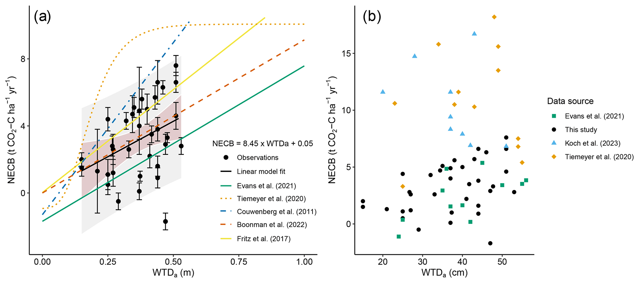
Figure 9 (a) Fitted linear model of measured mean annual water table depth (WTD_a) and net ecosystem carbon balance (NECB) of Table 2 compared to other empirical relations. NECB standard deviations are included as error bars, and the linear model is plotted with a 90 % prediction interval (grey shading) and a 95 % confidence interval for the linear fit (red shading). An overview of plotted models is presented in Table S3. Please note that Koch et al. (2023) found an identical fit to Tiemeyer et al. (2020), which is therefore not separately displayed. (b) WTD_a and NECB estimates of this study and from the literature. Only sites with similar land use (grassland) and a WTD_a within the range of our measurements (i.e. WTD_a not more than 5 cm outside of our WTD_a range) were selected for fair comparison.

Our NECBs also compare well with back-of-the-envelope emissions estimated from land subsidence rates, which range between 2 to 15 mm yr⁻¹ in the coastal peat soils in the Netherlands (Hoogland et al., 2012; van den Akker et al., 2008). With an average soil carbon content of 72 ± 10 kg m⁻³ at 80 cm depth across our locations (Fig. 2), and assuming that the carbon density profile from the surface up to 80 cm depth is roughly in equilibrium as decomposition due to drainage for agricultural use has been ongoing for at least 50 years (but at most sites over multiple centuries; e.g. Erkens et al., 2016), we infer emissions ranging between 1.5 and 11 $\mathrm{t}{\mathrm{CO}}_{\mathrm{2}}\text{-}\mathrm{C}{\mathrm{ha}}^{-\mathrm{1}}{\mathrm{yr}}^{-\mathrm{1}}$. These subsidence-derived estimates correspond well to our estimated NECBs (Fig. 9) and thus strengthen the presented approach to derive annual NECBs.

It is notable that our NECB estimates and the slope of the WTD_a–NECB relationship are on the lower side of those reported by Tiemeyer et al. (2020) and Koch et al. (2023) (Fig. 9). There are several potential explanations for differences between our results and those of others. Firstly, magnitudes of estimated NECBs and different NECB–WTD relationships may be related to differences in landscape, peat soil characteristics, peat decomposition state, and land-use history and practices (e.g. Evans et al., 2021; Tiemeyer et al., 2016). For example, in contrast to the aforementioned studies, the measurements presented in this paper are exclusively conducted on coastal peatlands, which often have a relatively high WTD, limited drainage, clay cover, and the ability for meticulous water management, whereas the studies mentioned earlier are compiled from measurements in a larger variety of peatlands with few data from coastal peatlands. The WTD_a–NECB relationships of Tiemeyer et al. (2020), Koch et al. (2023), and Evans et al. (2021) are based on NECBs from sites that widely differ in land use and are based on a WTD_a range that differs from the one on which our relationship was fitted, as the study of Tiemeyer et al. (2020) in particular, but also of Koch et al. (2023), contains NECBs from sites where the WTD_a lies far outside our measured range. These factors could affect the nature of the relationship, as at least some aspects of land use may have effects independent of those of WTD_a (Evans et al., 2021) and since deepening of the WTD_a likely has a finite effect on the oxygen penetration depth in the peat soil (Boonman et al., 2024b). Another factor that can affect the magnitude of the NECB and its relationship with WTD is the clay cover that is typical of the Dutch coastal peatlands (Koster et al., 2018). A clay cover limits the thickness of the layer of peat that is exposed to oxygen and hence limits mineralisation (Jansen et al., 2009). Additionally, a clay cover and mixtures of clay with peat may suppress mineralisation and related CO₂ emissions from peat (e.g. Deru et al., 2018) via (1) clay-labile carbon complexation that restricts degradation of the organic matter by microorganisms (Hassink, 1997; Torres-Sallan et al., 2017; Rumpel et al., 2015), (2) restricting oxygen transport to organic matter by decreasing soil pore sizes and increasing soil water content (Balogh et al., 2011), and (3) altering interactions with microorganisms and their enzymes (Turner et al., 2014). The presence of clay cover may thus contribute to observed differences between the magnitude of our NECBs and its relationship with WTD as compared to those from other European countries. Lastly, differences could be related to methodological issues, such as potential biases due to a changing microclimate in automated chambers (Maier et al., 2022; Oestmann et al., 2022; Yao et al., 2009), gap-filling uncertainties/choices (Liu et al., 2022), and choices in data-handling (Hoffmann et al., 2015; Shi et al., 2022). Different methods to determine NECBs have their own pros and cons (Liu et al., 2022) and should be used in as complementary a way as possible.

Although a sigmoidal function was used to model the WTD_a–NECB relationship on the entire dataset of Tiemeyer et al. (2020) and Koch et al. (2023), within our measured WTD_a range, a (pseudo)linear trend is evident in the subset of their data. To enable a fairer comparison between the WTD_a–NECB relationships based on our data and those from literature, we selected a subset of data from the Evans et al. (2021), Tiemeyer et al. (2020), and Koch et al. (2023) syntheses where WTD_a was within the range of our measurements (i.e. WTD_a not more than 5 cm outside of our WTD_a range; Fig. 9b). In addition, we only selected data from sites with similar land use to our sites, i.e. only grassland sites from Evans et al. (2021), only permanent or rotational grassland sites from Koch et al. (2023), and only sites where Lolium perenne was among the dominant species from Tiemeyer et al. (2020). By including data source as an interaction term with WTD_a in our linear mixed-effects model (LMM), we can isolate the WTD_a effect from potential differences in the slope or intercept of the compared relationships. As such, we can analyse whether combining our dataset with one from the literature adds evidence for an effect of WTD_a on the NECB (i.e. increase effect variance relative to error variance) and determine the evidence for a difference in slope and intercept between our WTD_a–NECB relationship and that of a given dataset from literature. When comparing our WTD_a–NECB relationship with the one based on the grassland sites (11 data points) of Evans et al. (2021), we found moderate evidence for an effect of WTD_a on the NECB (LMM: $F_{\mathrm{1},\mathrm{32}}=\mathrm{6.88}$; P=0.019) and no evidence for an effect of the data source (i.e. Evans et al., 2021, vs. this study) on the slope (LMM: $F_{\mathrm{1},\mathrm{32}}=\mathrm{1.02}$; P=0.32) and intercept (LMM: $F_{\mathrm{1},\mathrm{29}}=\mathrm{1.70}$; P=0.20) of the WTD_a–NECB relationship. On the contrary, when we did this analysis for a subset of data from Tiemeyer et al. (2020) (12 data points), we found no evidence for an effect of WTD_a on the NECB (LMM: $F_{\mathrm{1},\mathrm{40}}=\mathrm{1.09}$; P=0.30) and no evidence for an effect of the data source on the slope (LMM: $F_{\mathrm{1},\mathrm{40}}=\mathrm{0.06}$; P=0.81) and the intercept (LMM: $F_{\mathrm{1},\mathrm{30}}=\mathrm{1.21}$; P=0.28) of the WTD_a–NECB relationship. When comparing the WTD_a–NECB relationship based on the subset of Koch et al. (2023) with our relationship, there was also no evidence for an effect of WTD_a on the NECB (LMM: $F_{\mathrm{1},\mathrm{22}}=\mathrm{0.40}$; P=0.54), no evidence for an effect of the data source on the slope (LMM: $F_{\mathrm{1},\mathrm{22}}=\mathrm{2.35}$; P=0.14), and strong evidence for an effect of the data source on the intercept (LMM: $F_{\mathrm{1},\mathrm{19}}=\mathrm{9.27}$; P=0.0067) of the WTD_a–NECB relationship. Combining our data with the subset of Evans et al. (2021) in the LMM resulted in stronger evidence for an effect of WTD_a (P=0.019) than when testing the effect of WTD_a for each dataset independently (LMM: $F_{\mathrm{1},\mathrm{32}}=\mathrm{1.96}$; P=0.17 and LM: $F_{\mathrm{1},\mathrm{9}}=\mathrm{5.78}$; P=0.040 for our study and the subset of Evans et al., 2021, respectively). On the contrary, combining our data with the subset of Tiemeyer et al. (2020) or Koch et al. (2023) weakened the evidence for an effect of WTD_a as compared to only using our data in the LMM. These findings suggest that the relationship between WTD_a and NECB may not be consistent across all drained peatlands in use as grassland or under all environmental conditions. For example, it may imply that, compared to our dataset and the one of Evans et al. (2021), the German and Danish sites show greater variation in NECBs independent of WTD_a that may result from greater variation in land-use intensity or properties of the peat soil (see previous paragraph). Lastly, our results may imply that the various WTD–NECB relationships and magnitudes of NECBs are sensitive to methodological differences, as the data of Tiemeyer et al. (2020) and Koch et al. (2023) are based on campaign-wise measurements during the daytime with manual chambers, while our data (automated chambers) and the data of Evans et al. (2021) (eddy covariance) were collected with much higher temporal cover, which reduces the extent (and thereby uncertainty) of gap-filling and the need to predict nighttime CO₂ fluxes based on daytime measurements with opaque chambers. Future research should focus on comparing and validating the various methodologies – including effects of the extent of gap-filling – and causes of potential regional physical variation in NECB magnitudes.

3.5 Landscape-scale emissions

Upscaling emissions

To upscale emission estimates to those at the regional and national level, it is important that our results are included in mechanistic models that contain (geographic) data to account for things like spatial heterogeneity of peat types, peat depth, hydrology, year-to-year variation in weather conditions, type of measure (e.g. passive or active WIS), and management. Efforts are already being made to enable such upscaling of results using a multi-model ensemble (Erkens et al., 2022). Nevertheless, it becomes clear from our results that the application of WIS alone will be insufficient to achieve the targeted 95 % reduction in emissions in 2050. Hence, to achieve the emission reduction target, WIS can fit in as a (temporary) measure combined with more drastic rewetting measures. Lastly, when upscaling emissions and effects of management at the landscape scale, one should not only consider the direct land–atmosphere fluxes but also those from other landscape elements, such as ditches, that are affected by the mineralisation and management of the peat soil (as discussed below).

Waterborne export

Our NECBs determined via chamber measurements do not account for carbon fluxes via runoff; lateral subsurface flow; and emission of CH₄, CO, and volatile organic carbon. While emission of the latter three gases is likely negligible (e.g. Weideveld et al., 2021; Faubert et al., 2011; Aben et al., unpublished CO data), carbon losses via runoff, erosion, and lateral subsurface flow can be significant (Evans et al., 2016). This carbon is partly mineralised and emitted to the atmosphere in surrounding ditches and further downstream in the hydrological system.

Ditch emissions

Carbon and GHG emissions from ditches in managed peatlands can be substantial and are important on the landscape scale (Vermaat et al., 2011; Schrier-Uijl et al., 2014; Peacock et al., 2017; Piatka et al., 2024). For example, GHG emissions (CH₄, CO₂, N₂O) from ditches in drained peatlands in the north of the Netherlands were estimated to be 4.8 times larger on a per-area basis than those of the terrestrial peat, forming an estimated 20 % of landscape-scale emissions (Hendriks et al., 2024). Thus, to quantify carbon and GHG emissions from drained peatlands on the landscape scale, it is crucial to include emission estimates from ditches and downstream waters. Care should be taken not to include these emissions twice, as waterborne carbon export from the soil forms part of the carbon emission from ditches where the waterborne carbon export ends up.

Management

Similarly, effects of measures on waterborne exports and ditch emissions need to be quantified, as subsurface and shallow surface drains in managed peatlands likely stimulate losses of dissolved and particulate carbon and of dissolved GHGs, sulfate, and nutrients (Uusitalo et al., 2001; Vermaat et al., 2016; Kladivko and Bowling, 2021; Pickard et al., 2022). The latter two can stimulate anaerobic mineralisation of the organic ditch sediment while simultaneously contributing to external and internal eutrophication (Smolders et al., 2006) that in turn stimulates GHG emission (Beaulieu et al., 2019).

4 Conclusions

We presented the results of a novel and unprecedented CO₂ emission monitoring network for peatlands under intensive agricultural use (grassland) in the Netherlands, using automated transparent chambers. High-frequency measurements of CO₂ fluxes and supporting data (e.g. water table depth (WTD) and weather) provided us with up to 4 years of near-continuous, high-frequency measurements for 12 sites in the Netherlands, which we used to determine the annual net ecosystem carbon budget (NECB). The sites consisted of plots where water infiltration systems (WISs) were implemented, combined with nearby control plots. For the ranges in WTD considered in this study, we found a linear relation between NECB and annual (as well as summer) WTD as was presented in the literature before. However, a stronger relation was found between NECB and carbon exposure (Cexp), expressed as the amount of available soil carbon above the WTD. We therefore propose to use the carbon exposure rather than the WTD as a proxy for the NECB. Still, substantial variation in NECB could not be explained by these variables, and this deserves attention in future analyses. The WISs studied were proven to be effective in decreasing peatland CO₂ emissions in cases where they function as intended (i.e. raising the WTD). We found no evidence for an effect of WIS on the slope of the relation between NECB and WTD or on the slope of the relation between NECB and Cexp. The magnitude of our NECBs and the slope of the WTD–NECB relationship agreed well with some studies but not with all. This is potentially explained by regional differences in physical geographic setting, peat type, land-use history, and water management and/or by methodological differences, and it warrants further analysis. The large site-to-site and year-to-year variation calls for continuation of near-continuous, high-frequency measurements to further improve our understanding of the drivers of greenhouse gas emissions from peatlands in agricultural use.