Spatiotemporal variability of CO₂, N₂O and CH₄ fluxes from a semi-deciduous tropical forest soil in the Congo Basin

Tropical forests play an important role in the greenhouse gas exchange between the biosphere and atmosphere. Despite having the second largest tropical forest globally, the Congo Basin is generally understudied and ground-based greenhouse gas flux data are lacking. In this study, high-frequency measurements spanning 16 months from automated and manual fast-box soil chambers are combined to characterize spatiotemporal variability in soil greenhouse gas fluxes from a lowland tropical forest in Yangambi in the Congo Basin. Based on subdaily continuous measurements for CO₂, a total emission of 15.3 ± 4.4 $\mathrm{Mg}\mathrm{C}{\mathrm{ha}}^{-\mathrm{1}}{\mathrm{yr}}^{-\mathrm{1}}$ was calculated, with the highest fluxes at the start of the wetter periods and a decline in emissions during drier periods. For CH₄, the total uptake was −3.9 ± 5.2 $\mathrm{kg}\mathrm{C}{\mathrm{ha}}^{-\mathrm{1}}{\mathrm{yr}}^{-\mathrm{1}}$. Over the whole period the soil acted as a sink. However, sporadic emission events were also observed. For N₂O an emission of 3.6 ± 4.1 $\mathrm{kg}\mathrm{N}{\mathrm{ha}}^{-\mathrm{1}}{\mathrm{yr}}^{-\mathrm{1}}$ was calculated, which is higher than most previously reported tropical forest estimates. N₂O emissions decreased substantially during drier periods and emission pulses were detected after rain events. High spatial and temporal variability was observed for both CH₄ and N₂O, although less so for CO₂. Higher spatial variability was assessed through the manual measurements compared to the automated measurements. Overall, the tropical forest soil acted as a major source of CO₂ and N₂O and a minor sink of CH₄.

1 Introduction

The three most important biogenic greenhouse gases (GHGs) are carbon dioxide (CO₂), methane (CH₄) and nitrous oxide (N₂O). Although the increase in the atmospheric concentrations of these key GHGs since 1750 is unequivocally attributed to human activity (IPCC, Calvin et al., 2023), natural ecosystems also contribute significantly to atmospheric GHG budgets. Tropical forests play an important role in the GHG exchange between the biosphere and the atmosphere. Soils are the dominant terrestrial source of CO₂, and emissions from tropical forest soils are generally higher than from any other vegetation type, due to high soil moisture and temperature (Raich et al., 2002), higher gross primary production (GPP) of tropical forests compared to other forests and the larger proportion of GPP used for autotrophic respiration (Anderson-Teixeira et al., 2016). Soils can both produce and consume CH₄, but globally they are the largest biotic sink of atmospheric CH₄. Aerobic forest soils consume more CH₄ than other ecosystems but can become a source when inundated (Dalal and Allen, 2008; Dutaur and Verchot, 2007). Considering all natural sources of N₂O, soils are the largest contributor. In particular, emissions from tropical forest soils are 50 % higher than the global average for soils (Tian et al., 2020), as these tropical forests are generally nitrogen-rich systems (Brookshire et al., 2012; Hedin et al., 2009). Taking all biogenic GHGs together, the net global warming potential of tropical forest systems suggests them to be a small sink (Dalal et al., 2008), but large uncertainties remain as the spatial and temporal variabilities of tropical forest soil fluxes still remain poorly understood (Arias-Navarro et al., 2017; Courtois et al., 2019).

The difficulty in understanding the dynamics of soil fluxes lies in the multitude of controlling environmental factors and the complexity of the biological and physical mechanisms, which lead to high spatial and temporal variability (Courtois et al., 2018; Vargas et al., 2011). To date, the majority of soil flux measurements have been taken using manual static chambers, a technique that is able to capture spatial variability up to a certain degree but is labor-intensive and time-consuming. In addition, measurements are generally taken at weekly to monthly time intervals, thus not covering diurnal patterns and resulting in a lower accuracy than higher-frequency measurements (Barton et al., 2015). Also, no responses to precipitation events or nocturnal measurements will be present (Courtois et al., 2019; Vargas et al., 2011). Automated soil chambers, on the other hand, allow us to capture both diurnal and seasonal variability and even detect short-term variations or responses to rapidly changing environmental conditions. Nevertheless, a small number of chambers reduces the spatial scale of the measurements, leading to large uncertainties in the quantification of landscape GHG fluxes (Wangari et al., 2022). Combining automated chambers with fast-box measurements can address the spatial and temporal variability of soil GHG fluxes. However, the complexity of such a setup has limited its application in remote environments such as tropical forests, particularly in Africa.

Despite being the second largest tropical forest, the Congo Basin is generally understudied (Malhi et al., 2013). Recent studies have shown that the climatic conditions in the Congo Basin are already changing with an increasing length of the dry season (Jiang et al., 2019), warming (Dezfuli, 2017; Kasongo Yakusu et al., 2023), increasing numbers of extreme warm days and nights (Aguilar et al., 2009; Chaney et al., 2014; Kasongo Yakusu et al., 2023) and increasing precipitation intensity (Kasongo Yakusu et al., 2023). Climate change projections suggest that these trends will persist in the future (Karam et al., 2022; Kendon et al., 2019). As soil moisture and temperature are the main drivers of soil GHG flux dynamics, these shifts will directly affect the GHG budget (Ni and Groffman, 2018). Quantifying soil fluxes and understanding the role of temperature and moisture as drivers is key to assessing the future response of this biome to climate change. So far, only a handful of studies have reported in situ soil flux measurements from the Congo Basin (Fig. S1 in the Supplement and Table S1 in the Supplement). Studies such as Barthel et al. (2022) combined biweekly measurements from long-term observation sites with short-term daily measurement campaigns. However, to calculate more robust GHG budgets and to understand variability, data with a higher spatiotemporal resolution are needed.

In this study, a combination of automated and manual fast-box chamber measurements was used to quantify and understand the spatiotemporal variability of soil GHG fluxes in a semi-deciduous tropical forest in the Congo Basin. The objectives of the study are (1) to quantify annual budgets of soil CO₂, CH₄ and N₂O fluxes, (2) to evaluate the role of soil moisture and temperature as the main drivers of these GHG fluxes and (3) to analyze the spatiotemporal variability of soil GHG fluxes.

2  Methods

2.1 Study site

The study was conducted at the CongoFlux station (0°48^′52.0^′′ N, 24°30^′08.9^′′ E) (Fig. S2 in the Supplement) (Sibret et al., 2022) located in Yangambi on the right bank of the Congo River, approximately 100 km northwest of Kisangani in Tshopo Province of the Democratic Republic of Congo (DRC). The site is located in a semi-deciduous, lowland mixed-species forest with strongly weathered sandy clay loam and poorly drained soils dominated by Haplic Ferralsols (Gilson et al., 1956; Sibret et al., 2022; Fig. S10 in the Supplement). The soil in the top 30 cm has an average bulk density (BD) of 1.18 g cm⁻³, a H₂O pH of 4.0 and clay, sand and silt mass values of 30 %, 68 % and 2 %, respectively. The average carbon (C) content is 1.3 % and the average nitrogen (N) content is 0.22 % (Table S2 in the Supplement). The region has a warm and humid climate with a bimodal rain regime where two dry seasons (December–February and June–July) alternate with two wet seasons (March–May and August–November) (Kasongo Yakusu et al., 2023). The region experiences a mean annual rainfall of 1822.19 ± 214.80 mm and has a mean annual temperature of 25.0 ± 0.30 °C (Likoko et al., 2019). Within the CongoFlux site, four permanent forest plots (GEM – Global Ecosystem Monitoring – plots) of 1 ha (Fig. S2 in the Supplement) have been installed according to the RAINFOR-Gem field protocol (Marthews et al., 2014).

2.2 Climatic variables

Half-hourly precipitation at the site was measured by a tipping bucket (ARG100, Campbell Scientific Inc., Logan, Utah, USA) installed at 56 m on the tower used for eddy covariance measurements at the study site. Air temperature was measured using temperature and relative humidity sensors (HC2S3, Campbell Scientific Inc., Logan, Utah, USA) installed at a height of 2 m at the tower. Due to high lightning intensity at the site, power outages were frequent, resulting in several data gaps during the measurement period. Close to each automated chamber location, two water content reflectometers were installed (CS650, Campbell Scientific Inc., Logan, Utah, USA). The sensors were installed at depths of 5 and 15 cm at a distance of around 0.5 m from the collars to avoid disturbance of the soil in the chambers. Every minute the volumetric water content (VWC), soil temperature and electrical conductivity were logged. The water-filled pore space (WFPS) was then calculated following Eq. (1):

$$\begin{array}{}\text{(1)}& \text{WFPS}=\mathrm{100}\times \text{VWC}\times {\left(\mathrm{1}-{\displaystyle \frac{\text{BD}}{\mathrm{2.65}}}\right)}^{-\mathrm{1}}.\end{array}$$

Note: there is a large data gap from the end of March to the middle of July 2023 due to technical problems with the data logger.

2.3 Measurements of soil CO₂, CH₄ and N₂O exchange

2.3.1 Automated chamber measurements

At the CongoFlux site, nine custom-made dynamic automated chambers (Karlsruhe Institute of Technology) were installed just outside the 1 ha GEM plot CF1 (Fig. S2). The opaque chambers (0.5 m × 0.5 m × 0.15 m length, width and height) were controlled by a central steering unit consisting of a valve-tubing system connecting the chambers to two portable analyzers, one measuring CO₂ and CH₄ concentrations (LI7810, LI-COR inc., Lincoln, Nebraska, USA) and the other measuring N₂O concentrations (LI7820, LI-COR inc., Lincoln, Nebraska, USA). The nine chambers were placed randomly around the control unit at a maximum distance of 20 m. For each chamber, two collars were inserted 10 cm into the soil, and the chambers were relocated from one collar to the other every 2 or 3 weeks. Only chamber 6 was never relocated during the measurement period due to limited cable length. The chamber headspace air was circulated from the chamber to the analyzers and back to the chamber with 3.175 mm stainless-steel tubing. Before the analysis, sample air was dried to constant water vapor with a Nafion dryer. A portable computer was used for steering the valve system for consecutive chamber sampling, closing and opening chambers as well as data acquisition and storage.

The chambers were installed in May 2022 and were operated with a closure time of 15 min per flux measurement, followed by 2 min of purging with ambient air, resulting in one data point every 17 min. The flux rate was calculated using a linear fit. Measurements of CO₂, CH₄ and N₂O were discarded if the coefficient of determination (R²) of the CO₂ measurement was smaller than 0.9, and measurements of N₂O were also discarded if the R² of the N₂O measurement was smaller than 0.7, as these values indicated a systematic error such as imperfect closure of the chamber or a technical issue with the analyzers. Fluxes with units $\mathrm{mass}\mathrm{C}{\mathrm{h}}^{-\mathrm{1}}{\mathrm{m}}^{-\mathrm{2}}$ for CO₂ and CH₄ and $\mathrm{mass}\mathrm{N}{\mathrm{h}}^{-\mathrm{1}}{\mathrm{m}}^{-\mathrm{2}}$ for N₂O were then calculated using Eq. (2), which is a combination of the ideal gas law and scaling variables:

$$\begin{array}{}\text{(2)}& \text{flux}={\displaystyle \frac{\mathrm{d}q}{\mathrm{d}t}}\times {\displaystyle \frac{V\times P\times M_{\mathrm{w}}}{R\times T}}\times {\displaystyle \frac{\mathrm{60}}{A\times \mathrm{1000}}}.\end{array}$$

$\frac{\mathrm{d}q}{\mathrm{d}t}$ is the change in the mixing ratio over time (ppb min⁻¹ or ppm min⁻¹) resulting from the linear fit, V is the chamber volume (m³), P is the long-term average air pressure of the site (Pa), M_w = 12 for CO₂ and CH₄ and M_w = 28 for N₂O (g mol⁻¹), T is the average temperature during the closure time (°K), A is the surface area of the chamber (m²) and R is the universal gas constant ($\mathrm{J}{\mathrm{mol}}^{-\mathrm{1}}\mathrm{°}{\mathrm{K}}^{-\mathrm{1}}$). The data presented in this paper covered the period from 1 June 2022 to 26 September 2023, resulting in a coverage of 16 months, 25 209 data points for CO₂ and CH₄ and 18 635 data points for N₂O, divided equally between nighttime and daytime measurements. During precipitation events, the automated chambers continued to measure without interruption.

2.3.2 Fast-box measurements

The low number of automated chambers limited the spatial coverage of the soil flux measurements. Hence, the fast-box method was included to reference the results of the automated chambers to a larger study area. The four GEM plots at the CongoFlux site were divided into 25 subplots of 20 m by 20 m, and in each subplot one soil chamber was installed in March 2023 for measurement with the fast-box method (Hensen et al., 2013; Wangari et al., 2022). The chambers were PVC tubes with a diameter of 5.5 cm and a height of 13 cm, permanently inserted 3 cm into the soil. The four plots CF1, CF2, Mi2 and Mi5 were equipped with 25 chambers each, but 3 chambers were lost (2 in Mi2 and 1 in Mi5) and two locations were measured incorrectly (one in CF2 and one in Mi2), leaving a total of 95 chambers. During a period of 3 weeks from 4 to 28 August 2023, flux measurements of CO₂, CH₄ and N₂O were made during the day (between 08:00 and 18:00) in these plots using two portable analyzers, one measuring CO₂ and CH₄ (LI7810, LI-COR inc., Lincoln, Nebraska, USA) and one measuring N₂O (LI7820, LI-COR inc., Lincoln, Nebraska, USA). Plots CF1, CF2 and Mi5 were each measured six times during this 3-week period and plot Mi2 only five times. Two plots were measured per day with an average of 5 min between consecutive chamber measurements. To avoid consistently measuring the same chamber at the same time of day, the order in which the plots were measured was alternated and the route from chamber to chamber within one plot was changed every session. A closure time of 2 min was used, and the flux rate was calculated using a linear fit and Eq. (2). The quality control of these fluxes was similar to that of the automated fluxes, with the addition that fluxes with a low R² (<0.7) were also checked individually for their quality. Low R² values could be due to a low flux, and then the flux was set to 0. If the low R² was due to fluctuating concentrations, the measurement was discarded. The sizes of the fast-box chambers were smaller than those of the automated chambers and the number of chambers was larger, so the variation of the fluxes from the fast-box chambers would likely be larger than that of the automated chambers. However, as the processing of the fast-box data was the same as for the automated fluxes, we believe that the methods are compatible, and therefore we can use the automated fluxes for budget calculation and the fast-box measurements for referencing the spatial variability without any normalization or correction (Fig. S11 in the Supplement). No additional climatic variables or soil properties were measured in the four GEM plots.

3 Statistical analysis

For the automated chambers, the average flux was calculated as the arithmetic mean of all measurements from all chambers, and the average fluxes per chamber location (17 locations: two collars for each chamber except chamber 6) were calculated by taking the arithmetic mean of all measurements from each chamber location separately. The coefficient of variation (CV) for each chamber location was calculated as the standard deviation (SD) of the chamber location divided by the arithmetic mean of the chamber location. The CV between the chamber locations was calculated as the SD of the 17 average fluxes per chamber location divided by the arithmetic mean of the 17 average fluxes per chamber location. Daily fluxes were calculated by taking the arithmetic mean of all measurements from all chamber locations for each day, and the CV between the days was calculated as the SD divided by the arithmetic mean of all the daily fluxes. Annual budgets were calculated by adding the daily fluxes for 1 complete year. Days without flux measurements were filled using a linear interpolation if the gap was smaller than or equal to 10 consecutive days. For each of the 95 fast-box chambers, an average flux was calculated by taking the arithmetic mean of all measurements from one chamber during the measurement period. These fluxes were then averaged per plot, and the CV for each plot was calculated as the SD divided by the mean of the average fluxes per chamber. To investigate the effect of potential drivers of GHG fluxes, i.e., WFPS, soil temperature, air temperature and precipitation, linear mixed models were fitted using the nlme package, version 3.1-164 (Pinheiro et al., 2023), with the measurements from the automated chambers for each GHG. This was done using chamber number and collar number (i.e., location and position) as random intercepts and WFPS, soil temperature (Temp_soil), air temperature (Temp_air), accumulated rainfall over the past 30 min (Rain) and accumulated rainfall over the past 10 d (PrevRain_10 d) as fixed factors. To account for the temporal correlation in the data, a first-order autoregressive model was included in the fit (CorAR1). The CO₂ and N₂O fluxes were log-transformed, and the CH₄ fluxes were log-transformed after adding the minimum value of the fluxes. Fixed factors were removed from the fit if they had low t values, and removing them from the fit did not substantially increase the Akaike information criterion (AIC) and Bayesian information criterion (BIC) values of the fit. R² values were calculated according to Nakagawa and Schielzeth (2013) and partitioned following Stoffel et al. (2021). Collinearity of predictors was tested using the variance inflation factor (VIF). Effect sizes of the fixed factors are expressed as relative changes (%) in flux per unit increase in the fixed factor and are calculated by transforming the effect size y to exp (y)−1. Note that for CH₄ this relative change is calculated as a function of fluxes with the minimum flux added. The statistical difference between chamber locations for WFPS and soil temperature was tested with the Kruskal–Wallis test (nonparametric), followed by a Wilcoxon test. The statistical difference between hours for diel cycles was tested with the Friedman test (nonparametric with repeated measures), followed by a Wilcoxon test. Results were considered significant if the p values or Bonferroni p values were smaller than 0.05. To look into the effect of the high sampling frequency of the setup, a resampling procedure was carried out with the daytime measurements to simulate lower sampling frequencies with the same number of chambers by using a bootstrap with size 1000. The resampling scenarios were (a) one measurement per chamber every month, (b) one measurement per chamber every week, and (c) one measurement per chamber every day. The mean, minimum, maximum, interquartile range (IQR) and normalized interquartile range (NIQR) of the resulting budgets were calculated for each scenario. The NIQR was calculated as the IQR divided by the mean value and gives an indication of the spread of the resulting budgets compared to the mean value. More information about the resampling procedure can be found in the Supplement. All the statistical analyses were performed using the R software.

4 Results

4.1 Climatic variables

The total accumulated precipitation during the 16-month measurement period was 2181.7 mm, with the highest weekly accumulated precipitation of 133.7 mm in early September 2022 (week 36), followed by week 44 in early November 2022 and week 16 around mid-April 2023 (Fig. S3 in the Supplement). November 2022 was the wettest month of the measurement period, and December 2022 followed by May 2023 were the driest months (Table S3 in the Supplement). June 2023 had twice the rainfall of June 2022, which made June 2023 a considerably wet month for the short dry season, while May 2023 was drier compared to May 2022. August and September 2023 were dry for the start of the long wet season, each having around half of the amount of rainfall than the same months in 2022. The average hourly air temperature was 23.8 ± 2.5 °C, with an hourly minimum of 17.8 °C during the night and a maximum of 32.3 °C during the day (Fig. S3 in the Supplement).

The average WFPS at 5 cm depth was 27.8 ± 5.9 % with an average soil temperature of 23.9 ± 0.6 °C, while the average WFPS at 15 cm depth was 19.8 ± 4.1 % with an average soil temperature of 24.0 ± 0.5 °C. WFPS followed the seasonality of rainfall (Table S3) and ranged from minima at 5 and 15 cm of 11.3 % and 6.5 %, respectively, to maxima of 69.9 % and 42 % (Fig. S4 in the Supplement and Table S5 in the Supplement). Soil temperature ranged from minima at 5 and 15 cm of 21.7 and 21.9 °C, respectively, to maxima of 26.1 and 25.9 °C (Fig. S4 and Table S4 in the Supplement). A diel cycle marked soil temperature dynamics at both depths (Fig. S5 in the Supplement). At both depths, there were pronounced differences in WFPS and soil temperature between the chamber locations (Table S3).

4.2 Soil CO₂, CH₄ and N₂O exchange of automated chambers

CO₂ emissions from all automated chambers during the measurement period ranged from 37.2 to 463.1 $\mathrm{mg}\mathrm{C}{\mathrm{m}}^{-\mathrm{2}}{\mathrm{h}}^{-\mathrm{1}}$ (Table S6 in the Supplement), with an arithmetic mean, calculated with all the measurements, of 174.5 ± 50.1 $\mathrm{mg}\mathrm{C}{\mathrm{m}}^{-\mathrm{2}}{\mathrm{h}}^{-\mathrm{1}}$ and a median of 64.1 $\mathrm{mg}\mathrm{C}{\mathrm{m}}^{-\mathrm{2}}{\mathrm{h}}^{-\mathrm{1}}$ (Fig. S6a in the Supplement). The average emissions varied between the chambers, with the lowest average emission of 124.4 $\mathrm{mg}\mathrm{C}{\mathrm{m}}^{-\mathrm{2}}{\mathrm{h}}^{-\mathrm{1}}$ (chamber 8, collar 2) and the highest average emission of 263.1 $\mathrm{mg}\mathrm{C}{\mathrm{m}}^{-\mathrm{2}}{\mathrm{h}}^{-\mathrm{1}}$ (chamber 7, collar 1). Nevertheless, spatial variability over the entire measurement period appeared to be limited, with a CV between the chamber locations of 24 % (Table S6). The annual budgets, calculated for all 12 consecutive months, ranged from 15.0 to 15.1 $\mathrm{Mg}\mathrm{C}{\mathrm{ha}}^{-\mathrm{1}}{\mathrm{yr}}^{-\mathrm{1}}$ (Table S4).

The CH₄ flux during the measurement period ranged from −133.1 to 1209.0 $\mathrm{\mu }\mathrm{g}\mathrm{C}{\mathrm{m}}^{-\mathrm{2}}{\mathrm{h}}^{-\mathrm{1}}$ (Table S6) with an arithmetic mean, calculated with all the measurements, of −44.6 ± 59.1 $\mathrm{\mu }\mathrm{g}\mathrm{C}{\mathrm{m}}^{-\mathrm{2}}{\mathrm{h}}^{-\mathrm{1}}$ and a median of −54. $\mathrm{\mu }\mathrm{g}\mathrm{C}{\mathrm{m}}^{-\mathrm{2}}{\mathrm{h}}^{-\mathrm{1}}$ (Fig. S6b). Averaged over the entire measurement period, all chambers were a sink of CH₄, with the average uptake rates ranging from −85.0 $\mathrm{\mu }\mathrm{g}\mathrm{C}{\mathrm{m}}^{-\mathrm{2}}{\mathrm{h}}^{-\mathrm{1}}$ (chamber 5, collar 1) to −19.2 $\mathrm{\mu }\mathrm{g}\mathrm{C}{\mathrm{m}}^{-\mathrm{2}}{\mathrm{h}}^{-\mathrm{1}}$ (chamber 7, collar 1). Although the forest soil was a sink, each chamber position except collar 1 of chamber 5 experienced at least one period of high-CH₄ emissions (Table S6). Such an emission period had a duration of a couple of hours to 3 weeks. In total, 9.4 % of all the CH₄ measurements were CH₄ sources, with a maximum percentage per chamber location of 21 % (chamber 7, collar 1). The CV between the chambers was 48 %, indicating a strong spatial variability. The cumulative annual budgets ranged from uptakes of −3.7 to −4.1 $\mathrm{kg}\mathrm{C}{\mathrm{ha}}^{-\mathrm{1}}{\mathrm{yr}}^{-\mathrm{1}}$ (Table S4).

The N₂O emissions during the measurement period ranged from 2.8 to 841.5 $\mathrm{\mu }\mathrm{g}\mathrm{N}{\mathrm{m}}^{-\mathrm{2}}{\mathrm{h}}^{-\mathrm{1}}$ (Table S6) with an arithmetic mean, calculated with all the measurements, of 40.9 ± 46.4 $\mathrm{\mu }\mathrm{g}\mathrm{N}{\mathrm{m}}^{-\mathrm{2}}{\mathrm{h}}^{-\mathrm{1}}$ and a median of 25.4 $\mathrm{\mu }\mathrm{g}\mathrm{N}{\mathrm{m}}^{-\mathrm{2}}{\mathrm{h}}^{-\mathrm{1}}$ (Fig. S6c). The average emissions per chamber ranged from 22.9 $\mathrm{\mu }\mathrm{g}\mathrm{N}{\mathrm{m}}^{-\mathrm{2}}{\mathrm{h}}^{-\mathrm{1}}$ (chamber 8, collar 2) to 65.4 $\mathrm{\mu }\mathrm{g}\mathrm{N}{\mathrm{m}}^{-\mathrm{2}}{\mathrm{h}}^{-\mathrm{1}}$ (chamber 7, collar 2), and the relatively low CV of 30 % indicates that the spatial variability was limited over this extended period (Table S6). A cumulative annual budget for the N₂O measurements was not possible due to the 3-month data gap.

For CO₂, a diel cycle was observed with emissions increasing from 10:00 GMT+2 in the morning to 14:00 GMT+2 and decreasing again from 17:00 GMT+2 to 21:00 GMT+2 (Fig. S7a in the Supplement). For N₂O, a small diel cycle was also observed, with emissions increasing between 10:00 GMT+2 and 14:00 GMT+2 and decreasing again from 14:00 GMT+2 (Fig. S7b). For CH₄, no diel cycle was observed (Fig. S7c).

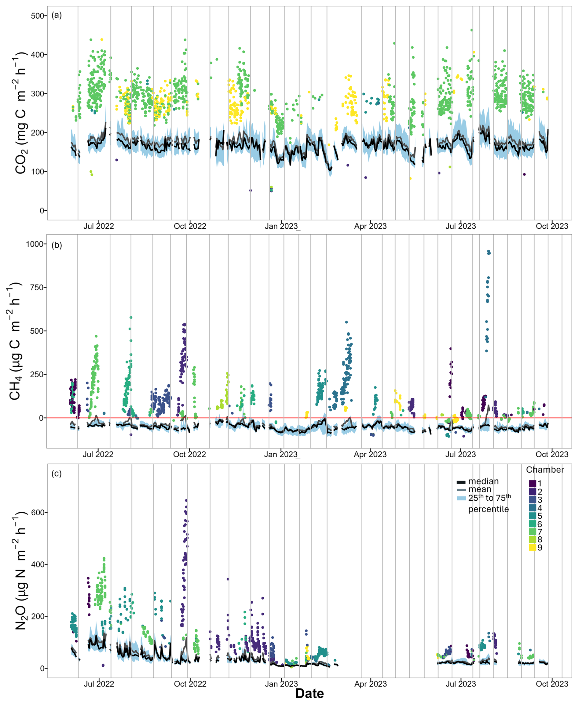
Figure 1 (a) CO₂, (b) CH₄ and (c) N₂O fluxes of all nine automated chambers over the whole measurement period. In black are the daily median values, in grey the daily averages and in blue the 25th to 75th quantiles. The coloured points are outlier values. Outliers have a distance to the 25th or 75th quantile value that is larger than 1.5 times the interquartile distance. Each colour represents one chamber. Vertical grey lines depict days when the chambers were replaced from one collar to another (Yangambi, DRC).

Daily fluxes were calculated by taking the arithmetic mean of all measurements from all nine chambers for each day. The mean daily flux for CO₂ was 174.0 ± 17.9 $\mathrm{mg}\mathrm{C}{\mathrm{m}}^{-\mathrm{2}}{\mathrm{h}}^{-\mathrm{1}}$ (Fig. 1a), with a CV between the days of 10 % and a range from 103.5 to 227.7 $\mathrm{mg}\mathrm{C}{\mathrm{m}}^{-\mathrm{2}}{\mathrm{h}}^{-\mathrm{1}}$. The low CV of the daily fluxes and the low CV of each chamber location individually (13 %–23 %; Table S6) indicate that the temporal variability for CO₂ was limited. The mean daily CH₄ flux was −44.7 ± 20.3 $\mathrm{\mu }\mathrm{g}\mathrm{C}{\mathrm{m}}^{-\mathrm{2}}{\mathrm{h}}^{-\mathrm{1}}$ (Fig. 1b), with a CV of 45 % and a range from −83.1 to 72.0 $\mathrm{\mu }\mathrm{g}\mathrm{C}{\mathrm{m}}^{-\mathrm{2}}{\mathrm{h}}^{-\mathrm{1}}$. There were 11 d with a positive mean flux. These positive fluxes were mostly dominated by one or two chambers showing elevated emissions covering periods of several days. The CV of the daily averages, including all the chambers, was relatively small compared to the CV values of the individual chamber locations (23 %–598 %; Table S6). The mean daily N₂O flux was 39.3 ± 27.7 $\mathrm{\mu }\mathrm{g}\mathrm{N}{\mathrm{m}}^{-\mathrm{2}}{\mathrm{h}}^{-\mathrm{1}}$ (Fig. 1c), with a high CV of 70 % and a range of 5.1–135.6 $\mathrm{\mu }\mathrm{g}\mathrm{N}{\mathrm{m}}^{-\mathrm{2}}{\mathrm{h}}^{-\mathrm{1}}$. The individual chamber locations also had high CV values (56 %–211 %; Table S6).

Reducing the sampling frequency of the measurements per chamber to one measurement every month and one measurement every week led to GHG budgets with NIQR values of 19.1 % and 9.1 %, respectively, for CH₄ and 13.6 % and 7.0 %, respectively, for N₂O, indicating a large spread of the calculated budgets (Table S10 in the Supplement and Fig. S8 in the Supplement). All three scenarios resulted in relatively low NIQR values for CO₂. Resampling the data with one measurement per chamber per day resulted in a NIQR value smaller than 3 % for all GHGs.

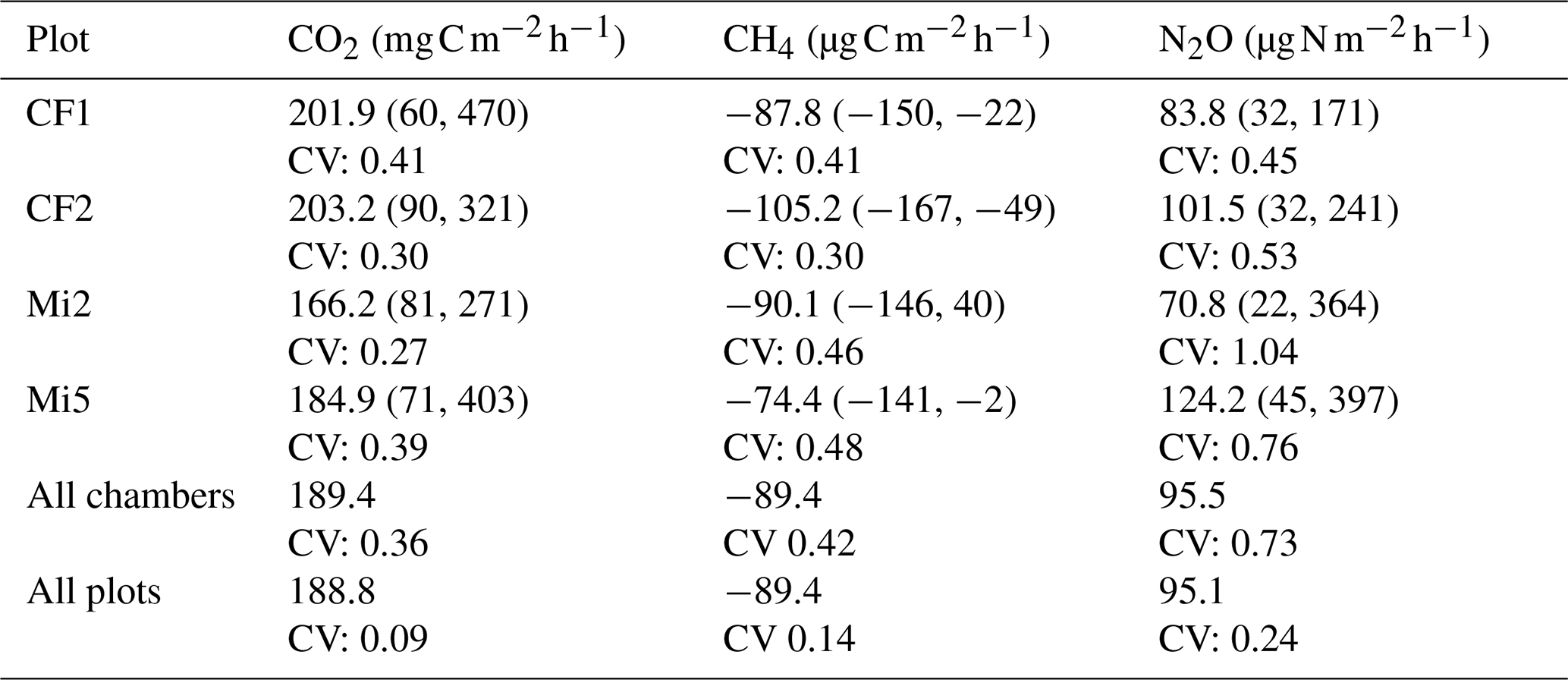
Table 1 For each of the 95 fast-box chambers, an average flux is calculated using all measurements from that chamber during the measurement period (4 to 28 August 2023). The values in this table are calculated using the average values per chamber. The average fluxes per plot for CO₂ ($\mathrm{mg}\mathrm{C}{\mathrm{m}}^{-\mathrm{2}}{\mathrm{h}}^{-\mathrm{1}}$), CH₄ ($\mathrm{\mu }\mathrm{g}\mathrm{C}{\mathrm{m}}^{-\mathrm{2}}{\mathrm{h}}^{-\mathrm{1}}$) and N₂O ($\mathrm{\mu }\mathrm{g}\mathrm{N}{\mathrm{m}}^{-\mathrm{2}}{\mathrm{h}}^{-\mathrm{1}}$) are shown together with the minimum and maximum values (mean (min, max)) and the coefficient of variation (CV). Also, the mean and CV are calculated for all the fast-box chambers together and for the averages of the four plots (Yangambi, DRC).

4.3 Soil CO₂, CH₄ and N₂O exchange of fast-box measurements

The average CO₂ flux of all 95 fast-box chambers was 189.4 $\mathrm{mg}\mathrm{C}{\mathrm{m}}^{-\mathrm{2}}{\mathrm{h}}^{-\mathrm{1}}$ (Table 1), a value close to the average of 176.3 $\mathrm{mg}\mathrm{C}{\mathrm{m}}^{-\mathrm{2}}{\mathrm{h}}^{-\mathrm{1}}$ of the nine automated chambers during the same period. The CV between the different plots was 9 % and the CV between the different chambers was 36 %, which was higher than the CV of 26 % between the automated chambers during the month of August. For CH₄, the average uptake measured with the fast-box method was −89.4 $\mathrm{\mu }\mathrm{g}\mathrm{C}{\mathrm{m}}^{-\mathrm{2}}{\mathrm{h}}^{-\mathrm{1}}$ with a CV of 42 %. Out of a total of 546 measurements for CH₄, 16 showed positive fluxes (3 %) distributed over 11 chambers in three different plots. Only one chamber had a positive flux over the entire measurement period. The average uptake rate measured with the fast-box chambers was higher than the average uptake measured with the nine automated chambers in August, which was −58.8 $\mathrm{\mu }\mathrm{g}\mathrm{C}{\mathrm{m}}^{-\mathrm{2}}{\mathrm{h}}^{-\mathrm{1}}$. The CV between the plots was 14 %, and the CV between the fast-box chambers was higher than the CV of the automated chambers during this period (35 %). For N₂O, the average flux was 95.5 $\mathrm{\mu }\mathrm{g}\mathrm{N}{\mathrm{m}}^{-\mathrm{2}}{\mathrm{h}}^{-\mathrm{1}}$, with high CV values of 73 % between the chambers and 24 % between the plots, indicating high spatial variability. The average flux measured by the fast-box chambers was much higher than the flux measured by the automated chambers throughout the entire measurement period. Due to a technical issue, the automated chambers had no flux measurements for N₂O during the month of August. However, the average flux measured with the automated chambers in July and September 2023 was 23.9 $\mathrm{\mu }\mathrm{g}\mathrm{N}{\mathrm{m}}^{-\mathrm{2}}{\mathrm{h}}^{-\mathrm{1}}$, which was only one-third of the value measured with the fast-box chambers. The CV between the fast-box chambers was much higher than the CV between the automated chambers in July and September (35 %).

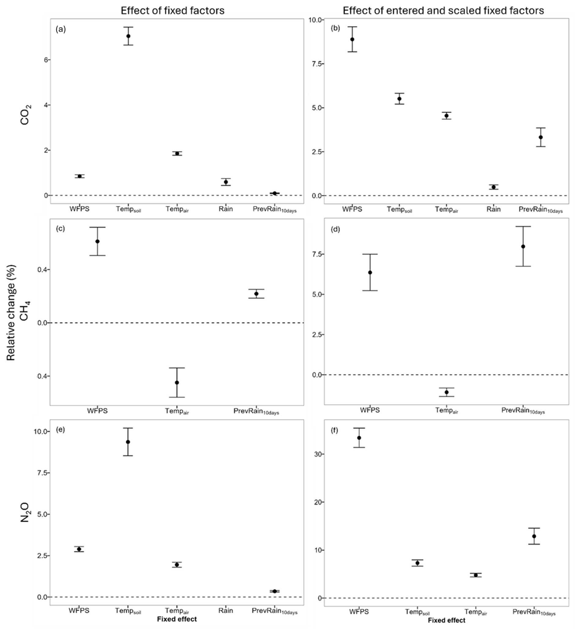
Figure 2 The relative fixed-effect sizes (%) for the fixed factors: water-filled pore space (WFPS, %), soil temperature (Temp_soil, °C), air temperature (Temp_air, °C), precipitation (Rain, mm per half-hour) and accumulated precipitation of the previous 10 d (PrevRain_10 d, mm) for the linear mixed-effect models of the automated chamber measurements (1 June 2022–26 September 2023) of the greenhouse gases (a) CO₂, (b) CO₂ with centered and scaled fixed factors, (c) CH₄, (d) CH₄ with centered and scaled fixed factors, (e) N₂O and (f) N₂O with centered and scaled fixed factors. The whiskers indicate the 95 % credible interval (Yangambi, DRC).

4.4 Main drivers of the GHG fluxes

For CO₂, all fixed factors were retained and all had a positive relationship with CO₂ fluxes (Fig. 2a and b, Table S7 in the Supplement). The fixed and random factors together explained up to 79 % of the variance of the fluxes. Similarly, only positive relationships were found between N₂O emissions and climatic variables (Fig. 2c and d, Table S9 in the Supplement). Rain was removed from the fit, and all the effects together explained 22 % of the variability. For CH₄, all the effects together explained 35 % of the variability. Both rainfall and soil temperature were removed from the fit. A positive relationship with CH₄ was found for WFPS and a negative relationship for air temperature (Fig. 2e and f, Table S8 in the Supplement). The model did not fit the data of the CH₄ measurements well, as the residuals showed heteroscedasticity and non-normality. WFPS had the largest relative effect size within the range of variability for all three models (Fig. 2b, d and f). The VIF for all the predictors in all the models was less than 2.

5 Discussion

5.1 Soil CO₂ emission

The average of all measurements from the automated chambers resulted in a carbon emission of 15.3 ± 4.4 $\mathrm{Mg}\mathrm{C}{\mathrm{ha}}^{-\mathrm{1}}{\mathrm{yr}}^{-\mathrm{1}}$. The gap-filled daily fluxes amounted to an annual budget of 15.1 $\mathrm{Mg}\mathrm{C}{\mathrm{ha}}^{-\mathrm{1}}{\mathrm{yr}}^{-\mathrm{1}}$ (Table S4). This value is higher than the previous estimate of 13.1 $\mathrm{Mg}\mathrm{C}{\mathrm{ha}}^{-\mathrm{1}}{\mathrm{yr}}^{-\mathrm{1}}$ by Baumgartner et al. (2020) in the DRC and more than double the amount of 6.3 $\mathrm{Mg}\mathrm{C}{\mathrm{ha}}^{-\mathrm{1}}{\mathrm{yr}}^{-\mathrm{1}}$ estimated by Werner et al. (2007) in Kenya. Our values are close to the 17.0 and 18.3 $\mathrm{Mg}\mathrm{C}{\mathrm{ha}}^{-\mathrm{1}}{\mathrm{yr}}^{-\mathrm{1}}$ estimated by Tchiofo Lontsi et al. (2020) for an undisturbed forest area in Cameroon. Our study shows that this Congolese forest soil is a larger CO₂ source than observed for tropical forest soils in French Guiana with emissions between 9.3 and 13.6 $\mathrm{Mg}\mathrm{C}{\mathrm{ha}}^{-\mathrm{1}}{\mathrm{yr}}^{-\mathrm{1}}$ (Courtois et al., 2018; Petitjean et al., 2019) and in Australia with emissions between 8 and 12 $\mathrm{Mg}\mathrm{C}{\mathrm{ha}}^{-\mathrm{1}}{\mathrm{yr}}^{-\mathrm{1}}$ (Kiese and Butterbach-Bahl, 2002). However, the emissions are comparable to those measured in Brazil of between 13.2 and 16.3 $\mathrm{Mg}\mathrm{C}{\mathrm{ha}}^{-\mathrm{1}}{\mathrm{yr}}^{-\mathrm{1}}$ (Sotta et al., 2007; Sousa Neto et al., 2011) and lower than the emissions reported for forests in Panama of 19.7 $\mathrm{Mg}\mathrm{C}{\mathrm{ha}}^{-\mathrm{1}}{\mathrm{yr}}^{-\mathrm{1}}$ (Pendall et al., 2010).

In this study, there was a low spatial variability between the automated chambers and between the fast-box chambers as well as a low temporal variability for CO₂ fluxes. This was also observed in other lowland tropical forests in Kenya by Werner et al. (2006) and in the DRC by Baumgartner et al. (2020). WFPS, soil and air temperature were the strongest drivers, each explaining up to 8 % of the variability in the data (Table S7). The random effect (chamber location and position) accounted for a large proportion of the variance. Both WFPS and soil temperature had a positive relationship with CO₂ flux, with WFPS having a larger relative effect size than soil temperature within their range of variability (centered and scaled factors) (Fig. 2). The positive relationship with WFPS is frequently observed in other studies in both the Congo Basin and other topical forests. During the early wetter period in July 2022, a first emission peak was observed with an increase in WFPS. However, there is a slight decline in the following wet months, although WFPS remains high (Fig. S9a in the Supplement). The same was observed in forests in Panama, where the decrease in emissions was partly attributed to a depletion of readily available C substrates and nutrients (Cusack et al., 2023). Baumgartner et al. (2020) suggest that CO₂ emissions in lowland forests in the Congo Basin may be limited by C availability, which could explain the decline in emissions after the first pulse of microbial activity at the beginning of the rainy season. A clear decrease in CO₂ emissions is also observed from the start of the drier period in mid-November 2022. The following relatively high peaks in emissions align with the increase in WFPS due to sporadic rain events. These emission peaks following rewetting events are common and are referred to as the Birch effect (Birch, 1958). With an increasing length of the dry season as expected from climate change predictions for the Congo Basin (Jiang et al., 2019), soil CO₂ emissions may decrease. However, with increasing rainfall intensity, which is also part of climate change projections (Kasongo Yakusu et al., 2023), the emission pulses after rewetting could become more frequent and severe. The positive relationship with soil and air temperature can explain the diel cycle of the CO₂ emissions found in this study (Figs. S5 and S7a). Peak soil respiration is reached before peak soil temperature, which indicates that the diel cycle is also sustained by increasing autotrophic respiration (Savage et al., 2013; Winnick et al., 2020).

5.2 Soil CH₄ uptake

For CH₄, the total uptake was −3.9 $\mathrm{kg}\mathrm{C}{\mathrm{ha}}^{-\mathrm{1}}{\mathrm{yr}}^{-\mathrm{1}}$ when using the arithmetic mean of all the measurements from the automated chambers, and the annual budgets amounted to an uptake between −3.7 and 4.1 $\mathrm{kg}\mathrm{C}{\mathrm{ha}}^{-\mathrm{1}}{\mathrm{yr}}^{-\mathrm{1}}$ (Table S4). This uptake is close to estimates from previous studies in the DRC with −3.5 $\mathrm{kg}\mathrm{C}{\mathrm{ha}}^{-\mathrm{1}}{\mathrm{yr}}^{-\mathrm{1}}$ (Barthel et al., 2022) but higher than the average uptake rates of tropical forest soils of −2.5 $\mathrm{kg}\mathrm{C}{\mathrm{ha}}^{-\mathrm{1}}{\mathrm{yr}}^{-\mathrm{1}}$ estimated by Dutaur et al. (2007) and −3.0 $\mathrm{kg}\mathrm{C}{\mathrm{ha}}^{-\mathrm{1}}{\mathrm{yr}}^{-\mathrm{1}}$ estimated by Dalal et al. (2008). In other African tropical forests, similar uptake rates were reported, e.g., for Cameroon with −4.3 and −2.5 $\mathrm{kg}\mathrm{C}{\mathrm{ha}}^{-\mathrm{1}}{\mathrm{yr}}^{-\mathrm{1}}$ (Tchiofo Lontsi et al., 2020) and −3.5 $\mathrm{kg}\mathrm{C}{\mathrm{ha}}^{-\mathrm{1}}{\mathrm{yr}}^{-\mathrm{1}}$ (Macdonald et al., 1998) and Kenya with −4.9 $\mathrm{kg}\mathrm{C}{\mathrm{ha}}^{-\mathrm{1}}{\mathrm{yr}}^{-\mathrm{1}}$ (Werner et al., 2007). Uptake rates of −2.6 $\mathrm{kg}\mathrm{C}{\mathrm{ha}}^{-\mathrm{1}}{\mathrm{yr}}^{-\mathrm{1}}$ were measured in Southwest China (Werner et al., 2006), −3.2 $\mathrm{kg}\mathrm{C}{\mathrm{ha}}^{-\mathrm{1}}{\mathrm{yr}}^{-\mathrm{1}}$ in Australia (Kiese et al., 2003), −3.8 $\mathrm{kg}\mathrm{C}{\mathrm{ha}}^{-\mathrm{1}}{\mathrm{yr}}^{-\mathrm{1}}$ in Brazil (Sousa Neto et al., 2011) and −1.1 $\mathrm{kg}\mathrm{C}{\mathrm{ha}}^{-\mathrm{1}}{\mathrm{yr}}^{-\mathrm{1}}$ in French Guiana (Petitjean et al., 2019).

Considerable spatial variability was observed, with CVs of 47 % and 42 % between the automated and fast-box chambers, respectively. The average uptake measured with the fast-box method was −89.4 $\mathrm{\mu }\mathrm{g}\mathrm{C}{\mathrm{m}}^{-\mathrm{2}}{\mathrm{h}}^{-\mathrm{1}}$ with a range of all measurements separately of −230.8 to 256.99 $\mathrm{\mu }\mathrm{g}\mathrm{C}{\mathrm{m}}^{-\mathrm{2}}{\mathrm{h}}^{-\mathrm{1}}$, while during the same period the automated chambers measured an average flux of −66.8 $\mathrm{\mu }\mathrm{g}\mathrm{C}{\mathrm{m}}^{-\mathrm{2}}{\mathrm{h}}^{-\mathrm{1}}$ with a range of −162.8 to 272.2 $\mathrm{\mu }\mathrm{g}\mathrm{C}{\mathrm{m}}^{-\mathrm{2}}{\mathrm{h}}^{-\mathrm{1}}$. This discrepancy may indicate that the nine automated chambers are not sufficient to cover the considerable spatial variability of CH₄ uptake, underlining the importance of a large spatial coverage. The CV of the daily averages (45 %) was relatively small compared to the CV of the individual chamber locations (Table S6), indicating that the temporal variability of the daily fluxes of all the chambers together was relatively small but that each chamber individually had a high temporal variability mainly caused by the periods of emissions. This high spatial and temporal variability is commonly found in studies in tropical forests (Barthel et al., 2022; Castaldi et al., 2020; Werner et al., 2007). Resampling the automated chamber measurements with a lower sampling frequency of once a month or once a week results in a large spread of possible CH₄ budgets (Table S10 and Fig. S8), which underlines the importance of a high sampling frequency.

The long-standing theory is that microbial methanogenesis can only occur in anoxic soils. Consequently, most weathered tropical forest soils are modeled as CH₄ sinks. However, sporadic CH₄ emissions have been measured in several studies. In the study by Werner et al. (2007), high WFPS and a crumbled soil structure, suggesting termite activity, were put forward as a possible explanation. Termite activity was also mentioned to explain CH₄ emissions in the study by Barthel et al. (2022). In a study in Costa Rica by Calvo-Rodriguez et al. (2020), high methane emissions were associated with heavy-precipitation events, while in the study by Castaldi et al. (2020) emissions were observed in well-drained soils and the authors suggested that the emissions may have been generated by anoxic hotspots of microbial activity within the overall aerobic soil. In this study, no clear evidence of termite activity was found at the chamber locations. The WFPS during emission periods ranged from 13.5 % to 70.5 % (Table S5), so the emissions did not only occur during wetter periods (Fig. S9b). In the case where the emissions are triggered by heavy-precipitation events, one would expect multiple chambers to emit during the same period, but in this study the timing of substantial CH₄ emissions was different for all the chambers. Even though WFPS and accumulated rainfall were the strongest drivers in the model, they only explained up to 4.8 % of the variability (Table S8). Overall, this suggests that the emissions in our study were also associated with sporadic anoxic microsites controlled by methanogenesis, as suggested by Castaldi et al. (2020) (Angle et al., 2017; Lacroix et al., 2023; Teh et al., 2005). A positive relationship between the flux and WFPS was found, which is frequently mentioned in other studies (Kiese et al., 2003; Werner et al., 2006; Werner et al., 2007; Sousa Neto et al., 2011), and a negative relationship between the flux and soil and air temperature was found. However, the relationship with soil temperature was insignificant.

5.3 Soil N₂O emission

The arithmetic mean of all the measurements resulted in a budget of 3.6 $\mathrm{kg}\mathrm{N}{\mathrm{yr}}^{-\mathrm{1}}{\mathrm{ha}}^{-\mathrm{1}}$. This value is close to the emission of 3.8 $\mathrm{kg}\mathrm{N}{\mathrm{ha}}^{-\mathrm{1}}{\mathrm{yr}}^{-\mathrm{1}}$ measured in Kenya (Werner et al., 2007). However, the value is higher than the tropical average of 3 $\mathrm{kg}\mathrm{N}{\mathrm{ha}}^{-\mathrm{1}}{\mathrm{yr}}^{-\mathrm{1}}$ estimated by Dalal et al. (2008), which is more than double that of the emissions measured previously in the DRC using static chambers (1.6 $\mathrm{kg}\mathrm{N}{\mathrm{ha}}^{-\mathrm{1}}{\mathrm{yr}}^{-\mathrm{1}}$) (Barthel et al., 2022) or in Cameroon (1.6 $\mathrm{kg}\mathrm{N}{\mathrm{ha}}^{-\mathrm{1}}{\mathrm{yr}}^{-\mathrm{1}}$) (Iddris et al., 2020). The value is also higher than the 2.3 $\mathrm{kg}\mathrm{N}{\mathrm{ha}}^{-\mathrm{1}}{\mathrm{yr}}^{-\mathrm{1}}$ estimated for Ghana (Castaldi et al., 2013) and the 2.9 $\mathrm{kg}\mathrm{N}{\mathrm{ha}}^{-\mathrm{1}}{\mathrm{yr}}^{-\mathrm{1}}$ estimated for the Mayombe forest in Congo (Serca et al., 1994). The emissions from the CongoFlux site are also higher than several other measurements in tropical forests, such as the 0.5 $\mathrm{kg}\mathrm{N}{\mathrm{ha}}^{-\mathrm{1}}{\mathrm{yr}}^{-\mathrm{1}}$ estimated in Southwest China (Werner et al., 2006), 2.4 $\mathrm{kg}\mathrm{N}{\mathrm{ha}}^{-\mathrm{1}}{\mathrm{yr}}^{-\mathrm{1}}$ estimated in eastern Amazonia (Verchot et al., 1999), 1.0 $\mathrm{kg}\mathrm{N}{\mathrm{ha}}^{-\mathrm{1}}{\mathrm{yr}}^{-\mathrm{1}}$ in French Guiana (Petitjean et al., 2019) and 1.0, 4.4 and 7.5 $\mathrm{kg}\mathrm{N}{\mathrm{ha}}^{-\mathrm{1}}{\mathrm{yr}}^{-\mathrm{1}}$ in Australia (Kiese et al., 2002, 2003).

The N₂O emissions have a high temporal variability, as the automated chambers have coefficients of variation between 56 % and 211 % (Table S6). Lowering the sampling frequency resulted in a large spread of possible N₂O budgets (Table S10 and Fig. S8), reducing the accuracy and precision of the estimated budgets (Barton et al., 2015). Emissions change significantly from year to year. The same months separated by only 1 year can differ in N₂O emissions by a factor of 4. This high temporal variability is consistent with most studies in tropical forests. In Australia, 2 consecutive years of measurements in the same region differed in N₂O emissions by a factor of 7 (Kiese et al., 2002, 2003). The CV between the fast-box measurements is high (73 %), which supports the high spatial variability of N₂O emissions (Barthel et al., 2022; Castaldi et al., 2013; Werner et al., 2007). The average flux of the fast-box chambers during the 3 weeks in August 2023 is 2 times as high as the average flux measured by the nine automated chambers during the entire measurement period and 3 times as high as the average flux measured by the automated chambers in July and September 2023. The large discrepancy between the measured fluxes from automated and fast-box measurements together with the low CV between the automated chambers but high CV between the fast-box chambers may indicate that the nine automated chambers are not able to capture the full spatial heterogeneity of the N₂O emissions.

WFPS is the strongest driver (Table S9) and has the largest relative effect size within its range of variability compared to other predictors (Fig. 2). The positive relationship fitted by the linear mixed model is found in several studies, confirming higher emissions during the wet season compared to the dry season (Iddris et al., 2020; Werner et al., 2007). Shortly after rain events, N₂O emissions increase rapidly and then decrease again slowly with decreasing WFPS (Fig. S9c). From January 2023, with the onset of the drier months, the high fluxes and peaked responses to increasing WFPS seem to disappear. This phenomenon was also observed by Kiese et al. (2003) in Australia, where it could have been associated with significant changes in the composition of the microbial community. With the onset of the early wet season around June and July, the emissions do not increase again. However, the fast-box flux in August is almost the same as the high average flux measured by the automated chambers around the same period in the previous year (June and July 2022). The large difference could therefore also to some extent be the result of altered conditions at the chamber locations due to the long deployment of the automated chambers at the same location. However, there was no clear difference in the other GHG fluxes during this period, and the location of the automated chambers was consistently changed between the collars, so this effect should be minor. The relatively low marginal R² of the fit suggests that there are other main drivers responsible for the large variability in N₂O emissions. In this study, we did not investigate other potential drivers, such as soil pH, microbial community composition or nutrient availability (Butterbach-Bahl et al., 2013), because sampling for these drivers, even at only a weekly frequency, was not trivial or feasible in this remote location.

6 Conclusions

Despite being the second largest tropical forest worldwide, the Congo Basin is still generally understudied. The few available soil GHG flux data differ in measurement techniques and have diverse resultant GHG budgets. In this study, a combination of automated and manual fast-box chamber measurements was used to quantify and understand the spatiotemporal variability of soil GHG fluxes in a semi-deciduous tropical forest in the Congo Basin. We believe that the results of this study provide a robust estimate representative of a large area within the Congo Basin, as the CongoFlux site makes up, in terms of vegetation, around 33 % of the entire basin, assuming a total size of 3.6×10⁶ km² (Shapiro et al., 2021). According to Baert et al. (2009), the main soil type of the CongoFlux site (Ferralsol) is also the dominant soil type of the DRC.

Overall, our observations confirm that tropical forest soils are a major source of CO₂ and N₂O and a sink of CH₄. With an emission of 15.1 $\mathrm{Mg}\mathrm{C}{\mathrm{ha}}^{-\mathrm{1}}{\mathrm{yr}}^{-\mathrm{1}}$, this study identifies the soil of this study area in the Congo Basin as a larger CO₂ source than most tropical forest soils previously reported in the literature. For N₂O, the emissions at the CongoFlux site were also higher than most emissions previously measured at tropical sites. With a global warming potential 265 times greater than CO₂, these high N₂O emissions should be taken into account in the GHG budget of tropical forests. High spatial and temporal variability was found for the CH₄ and N₂O fluxes, highlighting the need for additional measurement campaigns in the Congo Basin with an experimental design allowing large spatial coverage and a particularly high temporal sampling frequency when measuring soil fluxes. Lowering the sampling frequency of the measurements leads to a decline in the precisions of the estimated budgets. Soil and air temperature are positively related to CO₂ and N₂O emissions. Therefore, an increasing number of warm days and nights and general warmer weather conditions could lead to overall higher CO₂ and N₂O emissions from soils. CO₂ and N₂O emissions are lowest during drier periods. Therefore, the increasing length of the dry season could offset the effect of the increasing emissions with increasing temperatures. However, there are clear spikes in N₂O emissions after rainfall events and higher CO₂ emissions after the onset of the rainy season, and with an increasing precipitation intensity this could lead to higher and more frequent emission peaks for both CO₂ and N₂O, which in turn would increase the total GHG emissions from tropical forest soils. An increasing precipitation intensity could also lead to less uptake of CH₄, lowering the net uptake of −3.9 $\mathrm{kg}\mathrm{C}{\mathrm{ha}}^{-\mathrm{1}}{\mathrm{yr}}^{-\mathrm{1}}$ found in this study, but with the lower global warming potential of CH₄ this will only have a small influence on the total GHG emissions from forest soil. The net effect of climate change on the GHG budget of this ecosystem is still hard to predict and should be investigated further in appropriate warming and controlled rainfall studies.