Water usage of old-growth oak at elevated CO₂ in the FACE (Free-Air CO₂ Enrichment) of climate change

Predicting how increased atmospheric CO₂ levels will affect water usage by whole, mature trees remains a challenge. The present study investigates diurnal (i.e. daylight) water usage of oaks within an old-growth forest during an experimental treatment season (April–October, inclusive). Over the years 2017–2021, inclusive (years 1–5 of the experiment), we collected individual tree data from 18 oaks (Quercus robur L.) within a large-scale manipulative experiment at the Birmingham Institute of Forest Research (BIFoR) Free-Air CO₂ Enrichment (FACE) temperate forest in central England, UK. Diurnal tree water usage per day (TWU, L d⁻¹) across the leaf-on seasons was derived from these data. Equal tree numbers were monitored in each treatment: FACE infrastructure arrays (+150 µ mol mol⁻¹) of elevated CO₂ (eCO₂), FACE infrastructure control ambient CO₂ (aCO₂) arrays, and control “ghost” (no-treatment, no-infrastructure) arrays. TWU was linearly proportional to tree stem radius, R_b (∼ 3.1 L d⁻¹ mm⁻¹; 274 mm ≤ R_b ≤ 465 mm). R_b was also a very good proxy for projected canopy area, A_c (m²), which was linearly proportional to R_b (∼ 617 m² m⁻¹). Applying the stem-to-canopy relation implied a mean July water usage of ∼ 5 L d⁻¹ m⁻² of projected oak canopy in the BIFoR FACE forest. We normalised TWU by individual tree R_b to derive TWU_n (L d⁻¹ mm⁻¹). We report whole-season treatment effects, differing year on year, alongside July-only results. In the 2019 and 2021 seasons, after correction for repeated measures, there was a 13 %–16 %, reduction in eCO₂ TWU_n compared to aCO₂ TWU_n, with a marginal 4 % reduction in 2020, but these model results were not statistically significant. Control trees exhibited a significant 27 % increase in aCO₂ TWU_n compared to ghost TWU_n in the whole season in 2019, with lesser, nonsignificant fixed effects in 2020 and 2021. Several factors may have contributed: the installation or operation of FACE infrastructure; array-specific differences in soil moisture, slope, or soil respiration; or the mix of subdominant tree species present. Our results showing normalised per-tree water savings under eCO₂ align with sap flow results from other FACE experiments and greatly extend the duration of observations for oak, elucidating seasonal patterns and interannual differences. Our tree-centred viewpoint complements leaf-level and ground-based measurements to extend our understanding of plant water usage in an old-growth oak forest.

1 Introduction

Long-term manipulation experiments test how environmental drivers, such as increased atmospheric carbon dioxide levels, affect plants and ecosystems. Plant hydraulics are adapted to expected ranges of environmental parameters, with larger plants exhibiting greater resilience to wider parameter variation due to their ability to maintain water and food reserves. To maintain transpiration demands, trees accommodate themselves to diel variation in solar radiation, respiration fluctuation, high temperatures, and seasonal soil water deficits. Short-term mechanisms include stomatal regulation; the use of reserves, as evidenced by stem diameter variations (Sánchez-Costa et al., 2015); the use of stored plant water (Köcher et al., 2013); and the use of available water at variable soil depth (David et al., 2013; Flo et al., 20211; Gao and Tian, 2019; Nehemy et al., 2021). Development of resilient root structures (David et al., 2013; Flo et al., 2021) and minimisation of embolism mitigated by different xylem structures (Gao and Tian, 2019) may also occur. The ability of mature trees to withstand climate extremes may rely in part on using these buffering traits, which act to prevent permanent damage and maintain viability (Iqbal et al., 2021; Moene, 2014). This prompts the further question of how increasing atmospheric carbon dioxide levels will affect the hydraulic resilience of trees (Sect. 1.1 below).

The response of woody plants to drought varies considerably by species (Leuzinger et al., 2005; Vitasse et al., 2019), location (e.g. north versus south in Europe; Stagge et al., 2017), soil characteristics such as soil texture (Lavergne et al., 2020), and combinations thereof (Fan et al., 2017; Salomón et al., 2022; Sulman et al., 2016; Venturas et al., 2017). For example, large oak trees, the focus of the current study, may maintain their transpiration rates (compared to beech) during mild water stress but remain vulnerable to embolism and root damage (Süßel and Brüggemann, 2021).

1.1 Future-forest atmospheric carbon dioxide and water usage

Primary producers may respond to elevated CO₂ (eCO₂) levels by assimilating and storing more carbon, which happens during photosynthesis for plants containing chlorophyll. Global carbon and water cycle models (Guerrieri et al., 2016; De Kauwe et al., 2013; Medlyn et al., 2015; Norby et al., 2016) predict that, at least until the middle of the 21st century, trees and plants could potentially photosynthesise more efficiently, which may induce increased carbon storage. This could be beneficial for individual tree productivity. Stomatal regulation determines the trade-offs between carbon assimilation and water loss and, for a given leaf area and stomatal density, determines the rate and quantity of water usage seen in the stems of woody plants. Water usage at the tree level is, therefore, a strongly integrative measure of the whole-plant response to environmental drivers (such as temperature and precipitation) and experimental treatments (such as eCO₂).

Untangling the canopy water exchange and soil moisture hydraulic recharge dynamics within forest Free-Air CO₂ Enrichment (FACE) experiments can be complex, but responses to eCO₂ manipulations (including stepwise increases; Drake et al., 2016) inform our understanding of plant responses to climate change scenarios. Specific studies concerning transpiration and water savings of eCO₂ responses (Ellsworth, 1999; Li et al., 2003) have already improved the model predictions (De Kauwe et al., 2013; Donohue et al., 2017; Warren et al., 2011a), and here we seek additional evidence that will enable further advances to the predictive model capacity.

Experimental research into ecohydrological responses of old-growth and long-established deciduous forests to changing atmospheric CO₂ levels has been limited. The Web-FACE study (Leuzinger and Körner, 2007) reported on old individuals of temperate species and found that eCO₂ reduced water usage in Fagus sylvatica L. (dominant) and Carpinus betulus L. (subdominant) by about 14 % but had no significant effect on the water usage of Quercus petraea (Matt.) Liebl., the other dominant species present. The six Q. petraea included in Leuzinger and Körner's (2007) study were monitored to give measurements of accumulated sap flux (normalised against peak values in each tree) over two 21 d periods. Changes in water usage by long-established oak trees at eCO₂, measured for longer periods (greater than a month) across the leaf-on season, have not previously been reported.

Previous forest FACE experiments that reported tree/stand water usage (De Kauwe et al., 2013; Warren et al., 2011a), apart from Web-FACE, all constituted younger deciduous and mixed plantations of less than 30 years of age (Schäfer et al., 2002; Tricker et al., 2009; Uddling et al., 2008; Wullschleger and Norby, 2001; Wullschleger et al., 2002). Some of these eCO₂ treatments are long-term (durations of over 10 years in some cases), but all are limited in their period of monitoring sap flow (Schäfer et al., 2002). There are further (2010 onwards) sap flux studies of deciduous oak from studies that do not manipulate CO₂ but offer helpful data for comparison, for example within Europe (Aszalós et al., 2017; Čermak et al., 1991; Hassler et al., 2018; Perkins et al., 2018; Schoppach et al., 2021; Süßel and Brüggemann, 2021; Wiedemann et al., 2016) and in North America (Fontes and Cavender-Bares, 2019). Robert et al. (2017) have reviewed the hydraulic characteristics of oak species from multiple studies, which help us to place our results in context. Within the UK maritime temperate climate, only a few ecohydrological studies (e.g. Herbst et al., 2007; Renner et al., 2016) have previously considered the sap flow responses to water availability and drought for mixed-forest Quercus species.

The FACE method was developed to eliminate chamber and/or infrastructure influences (see, e.g. Pinter et al., 2000; Miglietta et al., 2001) and provides good control over CO₂ elevation levels (e.g. Hart et al., 2020). Nevertheless, few studies have explored the effects of the experimental infrastructure (e.g. on the resulting microclimate; LeCain et al., 2015). Disturbance of the vegetation was kept to a minimum while constructing the Birmingham Institute of Forest Research (BIFoR) FACE (Hart et al., 2020), but some clearing of ground flora and removal of coppice stems did occur, plausibly reducing competition and making more soil water available to the oaks. Other possible effects of infrastructure on water availability are discussed in Sect. 3.5.2.

1.2 Improving global vegetation models and questions of scale

Global vegetation models have been developed based on leaf-level plant knowledge alongside that of soil–tree–atmosphere exchange (e.g. Medlyn et al., 2015). These models have predicted reduced canopy conductance, G_s, and increased runoff in future climate scenarios, but an important gap has been identified between estimated and observed water fluxes (De Kauwe et al., 2013).

At the forest scale, studies of the effects of drought (2018–2019) on forested landscapes have shown that plant growth, stem shrinkage (Dietrich et al., 2018), and branch mortality may be affected for several years, especially for deciduous species in mature or old-growth forests (Salomón et al., 2022). At this forest scale (Keenan et al., 2013; Renner et al., 2016), there is also a more complex impact on the ecosystem and atmospheric demands as planetary-scale CO₂ levels increase, affecting boundary layer feedbacks.

In contrast to forest- and leaf-scale studies, canopy transpiration estimates from stem xylem sap flux (Granier et al., 2000; Poyatos et al., 2016; Wullschleger and Norby, 2001; Wullschleger et al., 2002) reflect how the whole canopy transpires rather than concentrating on individual leaf stomatal conductance to water. The present study is tree focused, bridging model-informing data gaps that were previously identified (De Kauwe et al., 2013; Medlyn et al., 2015). Tree-scale studies have provided essential data for calibration and validation of tree–water models (De Kauwe et al., 2013; Wang et al., 2016), identified key parameters driving responses to expected water shortages (Aranda et al., 2012), and compared species differences in mature tree responses to ambient aCO₂ (Catovsky et al., 2002) or eCO₂ (Catoni et al., 2015; Tor-ngern et al., 2015). Xu and Trugman (2021) have updated the previous empirical parametric and mechanistic model approaches to global vegetation modelling, reinforcing the need to use measured tree parameters (such as sapwood area) to improve model predictions.

Here we focus on whole-tree species characteristics and link these parameters to diurnal (i.e. daylight) tree water usage per day (TWU, L d⁻¹) from marginally intrusive stem xylem sap measurements. These measurements provide highly time-resolved data of plant water usage for several years with minimal maintenance. Heat-based measurement techniques (Forster, 2017; Granier et al., 1996; Green and Clothier, 1988) have been used over the past 40 years for measurements of plant xylem hydraulic function (Landsberg et al., 2017; Steppe and Lemeur, 2007), with automated data capture enabling increasingly realistic models of whole-tree xylem function.

1.3 Objectives, research questions, and hypotheses

This study provides new data from a field-based FACE environmental manipulation experiment to characterise seasonal and inter-year patterns of daily water usage by old-growth oak trees under eCO₂. We test for significant differences between treatments within these water usage distributions and patterns and take into account the effect of FACE infrastructure. The paper relates diurnal tree water usage per day (TWU, L d⁻¹) to measurable tree traits (stem radius, R_b (mm), and canopy area, A_c (m²)) and examines variation in TWU with environmental drivers and soil moisture. It also examines the limitations of water usage measurement by compensation heat pulse (HPC) sap transducers.

The following specific research questions and associated hypotheses are considered.

1. Is there a measurable difference in TWU distribution under eCO₂ compared to (infrastructure-containing) ambient CO₂ control (aCO₂) across the seasonal cycle?

   Hypothesis 1 – a detectable eCO₂ treatment effect is present, reducing TWU for eCO₂ trees.

2. Does the presence of FACE infrastructure measurably affect TWU?

   Hypothesis 2 – TWU is greater in the presence of FACE infrastructure.

2 Materials and methods

2.1 BIFoR FACE

At the BIFoR FACE experiment in central England, UK (Hart et al., 2020), we investigate soil–plant–atmosphere flows and fluxes of energy and water (Philip, 1966). We monitor soil–xylem–stomatal responses to aCO₂ and eCO₂ levels in a mixed-deciduous temperate forest of approximately 180-year-old trees. The eCO₂ treatment represents conditions expected by the middle of the 21st century (see the shared socioeconomic pathways (SSPs) in IPCC, 2021). This long-term experiment presents a rare opportunity to gain new insight into the complexity of water usage of old-growth forest trees in a changed atmospheric composition. BIFoR FACE is unique amongst free-air experiments in its ability to study the ecohydrology of these pedunculate oaks (Quercus robur L., subsequently abbreviated as oak) under eCO₂.

The BIFoR FACE facility is in Staffordshire (52.801° N, 2.301° W), England, UK (Fig. 1). The forest is a circa 1840 plantation of oak with a Corylus avellana (hazel) coppice. Naturally propagated Acer pseudoplatanus (sycamore), Crataegus monogyna (hawthorn), Ilex aquafolium (holly), and smaller numbers of woody plants of other orders (e.g. Ulmus (elm), Fraxinus (ash)) of varying ages up to circa 100 years old are also present. Some subdominant trees, e.g. sycamore, hawthorn, and elm, impinge on the high, closed canopy. Each experimental array, ∼ 30 m in diameter, was selected to contain ∼ six live oak trees. There are nine experimental arrays: three with infrastructure injecting eCO₂ (+150 parts per million by volume (ppmv)), three infrastructure controls injecting aCO₂ (∼ 410 to 430 µ mol mol⁻¹ for 2017–2021, inclusive), and three “ghost” (no-treatment, no-infrastructure) controls. Data were collected for all three FACE facility treatments. Here we concentrate on oak, the dominant species, with sap flow monitoring restricted to 2 oaks in each of the nine experimental arrays, totalling 18 trees.

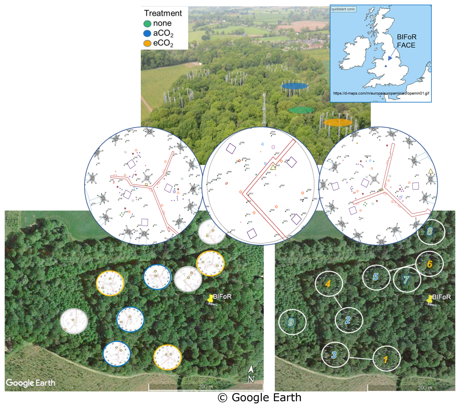
Figure 1 BIFoR FACE research woods showing three treatment types and nine arrays. Top left – aerial view, adapted (with permission) from Ch. 7, Fig. 7 of Bradwell (2022). Top right – location of BIFoR FACE within the British Isles; the map is cropped from https://d-maps.com/m/europa/europemin/europemin01.gif (last access: 7 November 2022). Middle – examples of three arrays, one per treatment, showing small brown rings within arrays to indicate the oak trees monitored for xylem sap flow. Bottom left – oak positions in all arrays. Bottom right – infrastructure treatment arrays are paired for similar soil conditions.

The climate at the site is temperate maritime, with a pre-experimental mean annual temperature of 9 °C and mean annual precipitation of 690 mm.

We compare individual tree sap flux and TWU responses under the three treatments across the leaf-on seasons for these early experimental FACE years, looking at within-year and inter-year relationships. We also describe daily, monthly, and seasonal changes to sap flux and TWU for mature oak over 5 years and discuss how these results, from our tree-centred viewpoint, will improve our understanding of future-forest water dynamics of old-growth forest, contributing to the development of more realistic ecohydrological vegetation, soil, and landscape models.

Typical experimental arrays showing target oak trees are shown in Fig. 1. Parameter symbols used in this paper are covered in Appendix A, Table A1. The term “sap flow” is used generally when referencing heat transducer methods to measure the water movement through sapwood. The use of the terms “sap velocity” and “sap flux” is defined in Tables A1 and A2. These usages (from Lemeur et al., 2009; Tranzflo Manual, 1998) may differ from other authors' usage (e.g. Poyatos et al., 2021).

2.2 Measurements overview

Our experiment is a triple-replicated (array) between-group (treatment type) design within which we selected our sample of oak tree individuals for continuous monitoring. There are three manipulation types, from which we select two individual trees in each array (a total of sample six trees per treatment). The individuals were not changed during the continuous experiment, nor were the measurement devices removed.

We report data from five treatment seasons, July 2017 to the end of October 2021. We focus on diurnal (i.e. daylight) responses within our experimental treatment season of April–October, inclusive. Sap flux and TWU datasets for the 18 oaks are calculated from half-hourly tree stem sap flow measurements derived from HPC transducers. TWU data is accumulated from sap flux and then analysed monthly within the treatment season across each year. For all xylem-sap-flux-monitored oak trees, tree identification, treatment type, array number, and stem circumference and average R_b at the probe set insertion point are shown in the Supplement (Table S1).

Figure S1 shows the key measurement points related to tree hydraulics in this project. This sap flow study is supported by other core environmental (detailed below) and soil data available at our FACE experimental site (MacKenzie et al., 2021). Table S2 shows instrumentation types and related parameters used for analysis within this paper, which are described below.

We experienced early leaf-on herbivory attacks on oaks by European winter moth larvae, especially in 2018 and 2019 (Roberts et al., 2022), which decreased leaf area by 20 %–30 % and affected the timing of canopy closure. A longer dry period occurred in the meteorological summer of 2018 (Rabbai et al., 2023), with wide variation in summer monthly precipitation across the study years. From 2016 to 2021 (treatment years), these 6-year averages (MAP 750 mm, MAT 10.6 °C) measured at or near the site were higher (+9 % and +18 %, respectively) than the previous reported means (see above). Precipitation is further discussed below, with additional detail in the Supplement (Table S14, Figs. S10, S14, S15, and S16).

2.3 Seasonal definitions

We define a plant hydraulic year as being from the start of the dormant season (1 November) to the end of senescence (31 October). The 7 months of CO₂ treatment per year (with 6 months of leaf-on photosynthesis) do not easily divide into standardised meteorological seasons (spring, summer), so we define our months of interest, including non-treatment months, as shown in Table 1. The table includes 2 months, March to April, of pre-leaf growth when oak sap starts to rise.

Table 1 Definition of treatment season periods and dates for oak phenology at BIFoR FACE according to Nature's Calendar criteria for the years 2017–2021, inclusive (canopy closure data were not recorded). Dates within parentheses during dormant periods are not exact due to limited site visits by authors. First tint is also recorded in the year 2016 on 4 October.

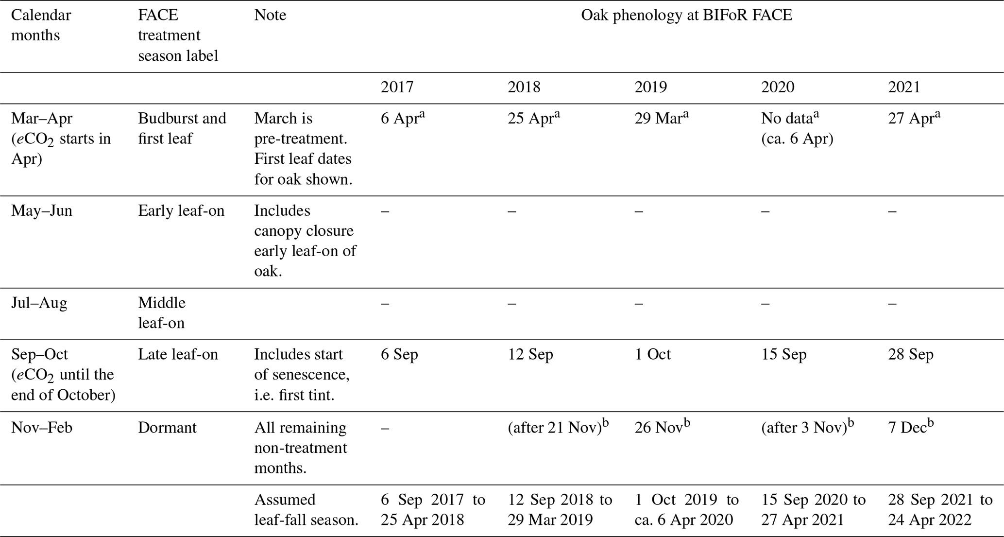
The terms budburst, first leaf, first tint, and bare tree are used as defined by Nature's Calendar. ^a On-site first leaf data (not obtained in 2020 due to the Covid-19 pandemic: 6 April 2020 was noted as budburst; unverified first leaf is recorded as 24 April 2020). Note that separate records of leaf-fall season are recorded for LAI calculation purposes, as Nature's Calendar data do not discriminate first leaf fall by leaf colour. ^bFirst bare-tree date recorded. The Nature's Calendar link is https://naturescalendar.woodlandtrust.org.uk/ (last access: 29 January 2022). PhenoCam data are additionally available for all years (https://phenocam.nau.edu/webcam/roi/millhaft/DB_1000/, last access: 10 July 2023).

Season length, between first leaf and full senescence/the first bare tree, is relatively constant at 8 months for the years studied, although the start and end vary year on year (Table 1). Canopy greenness, recorded as part of the PhenoCam network (https://phenocam.nau.edu/webcam/roi/millhaft/DB_1000/, last access: 10 July 2023), shows a very rapid decline towards wintertime values from the beginning of November. We have not collected phenology data specific to our target trees to capture any variability amongst individuals (see Sass-Klaassen et al., 2011).

2.4 FACE and meteorological measurements

Local precipitation (from a mixture of sources including meteorological towers; see MacKenzie et al., 2021) was recorded. Treatment levels of eCO₂, the diurnal CO₂ treatment period, top of canopy air temperature (T_a; °C), and total solar radiation (TG; W m⁻²) (see Figs. S9 and S11) were available from the FACE control system (Hart et al., 2020; MacKenzie et al., 2021). Data were averaged across the six infrastructure arrays for TG and T_a, as the ghost arrays have no FACE measurements. Set point levels of ambient CO₂ were used to control treatment application in the eCO₂ arrays. There are also increases in the ambient levels of CO₂ present across the years of this study of about 3.5 ppmv yr⁻¹. The enrichment level is unique to BIFoR FACE at +150 µ mol mol⁻¹, tracking the increasing ambient levels of CO₂ present across the years of this study (∼ 410 to 430 µ mol mol⁻¹ for 2017–2022; Fig. S12) and altering the relative percentage change in eCO₂ : aCO₂ year on year by about 1 %, from 36 % (beginning of 2018) down to 35 % (end of 2021) (Fig. S12).

Water inputs of throughfall precipitation under the oak canopy (within 2 to 3 m of an oak stem and situated near a soil moisture monitoring position) were measured in all arrays, with all transducers positioned under an oak canopy near the stem. Pre-treatment (2015–2017 for all arrays) and on-site soil and throughfall data were used to characterise the site. Supplementary (2018 onwards) throughfall and/or soil monitoring sites were added (see MacKenzie et al., 2021). These data were captured by the same CR1000 data logger as the sap flow data. Given the frequency of rainy days during the treatment season, we have not segregated our analyses into rainy and dry days.

2.5 Tree selection

Variation between individuals in treatment plots can arise from their precise location within an array or from inherent (biological) variation between individuals, as well as from different treatments (Chave, 2013). This individual-tree experiment design aims to minimise atypical variation. Accordingly, the following criteria were used to select trees for sap flow monitoring:

• canopy cover completely within the array (eCO₂ and aCO₂ arrays);

• central location within the plot near the logger and adjacent to access facilities at height (eCO₂ and aCO₂ arrays for sampling and porometry access);

• straight stem, preferably with little epicormic growth;

• no large dead branches within the canopy that might affect the comparative biomass of the tree;

• unlikely to experience seasonal standing or stream water at the base.

Target oak trees conforming to the above were chosen for monitoring to suit physical limitations of the transducer-to-logger constraints (e.g. cabling lengths including extensions to the same).

2.6 Tree characteristics

All oak trees were of a similar height (∼ 25 m). Stem circumference (metres) at the insertion height of probes was measured at installation (from 2017 onwards) and in subsequent winters (January 2020–February 2022). The range and mean-per-treatment values in 2022 are tabulated (Tables S1 and S3). We note that tree size will affect TWU (Bütikofer et al., 2020; Lavergne et al., 2020; Verstraeten et al., 2008).

Canopy spread of all target oak trees was measured, using a clinometer and a laser distance device to identify canopy extent (canopy radius) at the four cardinal compass points (Hemery et al., 2005). We assume that the two-dimensional canopy area, A_c (m²), derived from the mean canopy diameter plus stem diameter is correlated with canopy transpiration. Canopies were first measured around installation dates (2017–2018) and then repeated for all oaks in early 2022. On the second occasion in 2022, we measured the asymmetry of each tree stem across the probe set cardinal directions (east–west) and at right angles to this (north–south) to check the mean R_b value for sap flux calculations.

2.7 Xylem sap flux

Details of the xylem sap flux measurement method and associated calculations are provided in Appendix A, Table A2, and Appendix C. Each target oak tree had two probe sets, facing east and west (Fig. S2). Appendix B discusses the lower detection limit that the time-out characteristic places on this set of HPC data and on the consequent results. The validity of high value extrema is considered within our analysis.

To determine the whole-tree sap flux, two tree characteristics were used: (a) tree stem circumference at the insertion point (to determine the stem radius) and (b) bark thickness. From these data, we derived the tree stem cambium radius at the insertion point (R, m) and subsequently the heartwood radius (H, m) from the sensor spacing. H could not be determined from 10 cm cores, as these were not taken for all sap trees monitored.

The xylem sap flow installations in target trees commenced in January 2017. All ghost oak trees provided data from August 2017, and commissioning of all 18 oak trees was completed by autumn 2018. All oak sap flow installations were successful, and a total of 12 259 d of individual tree data (770 667 diurnal sap flux measurements across all months) were processed for the 2017–2021 TWU analysis. Data gaps in the earliest installations affected 4 of the 36 probe sets installed in four trees from August 2017 until September 2019.

With respect to the quality assurance of raw HPC data, commissioning and failure data were recorded for each probe set. This enabled a combination of data file amendment (especially for the earliest installations on separate loggers) and post-capture filtering to eliminate periods of invalid data for each probe set.

Example diel sap flux patterns for the ghost arrays in August 2019 (before filtering to eliminate nocturnal data) are shown in Fig. S3a, with east- and west-facing probe sets in each column. The sap flux data still show the minimum threshold levels (which vary by tree size) determined by the post-heat-pulse sampling period. It is noticeable that there is often a circumferential imbalance in xylem sap flux in the east (left-hand column of Fig. S3a) and west (right-hand column of Fig. S3a) probe set position data, which reflect the asymmetry in growth ring width around the stem typical in these old oak trees. The blank panels represent faulty probes (in two ghost trees), which were corrected by autumn 2019.

To compare individual tree responses across the leaf-on seasons, we filter the half-tree sap flux parameters using the solar azimuth and solar radiation parameters captured from the FACE control instrumentation (solar azimuth >−6° and solar radiation >0 W m⁻²) to give just daylight (diurnal) data. Where both probe sets in a tree are providing good data, a mean whole-tree sap flux is derived and incorporated into the TWU (Fig. S3b). We had sufficient whole-tree data to exclude single-probe-set results.

There are day-to-day differences in TWU between trees in our study (e.g. Fig. S3b), even though all of them experience very similar environmental conditions, and this pattern is replicated across the three treatment types. The TWU data reported here compare well to results from other studies (Table S4 in David et al., 2013; Sánchez-Pérez et al., 2008; Tatarinov et al., 2005; Baldocchi et al., 2001).

2.8 Data processing, visualisation, and analysis

Manually collected data were preprocessed as .csv files for import to R (R version 4.4.1, 2024). Raw data from data loggers were processed, visualised, and consequently analysed using R and R Studio (Posit Team, 2024) on Windows 10 x64 (build 1909). Most figures in the Results section were created using the R package ggplot (Wickham, 2016). Other standard packages (e.g. lubridate) are listed in the R scripts accompanying the data (see “Data availability” section below). Regressions between R_b and water usage and between R_b and A_c were calculated using the lm function. Box and whisker plots to visualise seasonal and monthly differences in sap flux and water usage between trees and treatments were generated in ggplot, where standard Tukey (McGill et al., 1978) percentiles (median + interquartile range), whiskers (1.5 ⋅ IQR from each hinge, where IQR is the interquartile range), and points for outliers are used. LOESS (locally estimated scatterplot smoothing) was used for exploratory analysis of the time series data (e.g. Fig. S13), an approach that does not rely on specific assumptions about the distributions from which observations are drawn. Levene tests (Levene, 1960) were carried out using leveneTest from the car library. Analysis of variance (ANOVA) models were used to test hypotheses with the functions anova and summary. The autoplot function from the ggfortify library was used to test the assumptions of normality of the ANOVA residuals. Nonparametric Wilcoxon rank-sum tests were used to check the ANOVA results, using wilcox.test. Generalised linear mixed-effect models (GLMMs) (using the function glmer from lme4) were selected to assess the random effects of the longitudinal (time-based) and individual (tree) repeated measures and estimate corrected fixed effects of treatments. The summary and tab_plot functions (from the sjPlot package) were used to extract the results.

3 Results

This section is organised as follows. We first report general characteristics of the distribution of sap flux (Sect. 3.1) and then develop relationships between TWU; R_b; and projected canopy area, A_c (Sect. 3.2). Subsequently, we discuss the characteristics of TWU_n (L d⁻¹ mm⁻¹, Sect. 3.3), which we use to test for treatment effects in an analysis of variance (Sect. 3.4). We provide a qualitative discussion of the effects of seasonal weather in the Supplement Appendix.

3.1 Sap flux within the season and between years

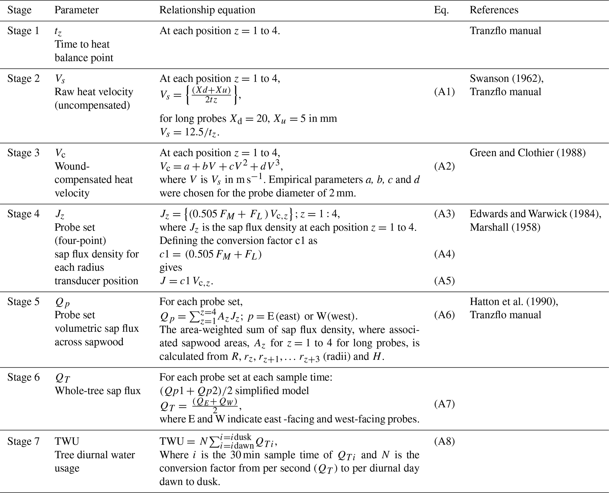
Diurnal stem sap flux responses to canopy photosynthetic demand typically exhibit increased sap flux from dawn to around midday (UTC – local solar time at the site), with an approximately symmetrical decrease until dusk (Fig. S3). Figure 2 shows the diurnal sap flux (i.e. Q_E and/or Q_W data derived from each east- and west-facing probe set installed per tree) in each of three ghost array oaks (selected for the smallest, largest, and medium-sized stem; see Tables S1 and S3) for the treatment seasons from 2018 to 2021. The partial year 2017 is not shown. We have retained Q_E and Q_W to show more of the short-term variability rather than averaging to Q_T, as single-probe-set results demonstrate circumferential imbalance (Fig. S3a), which can change with the year of operation (Fig. S4).

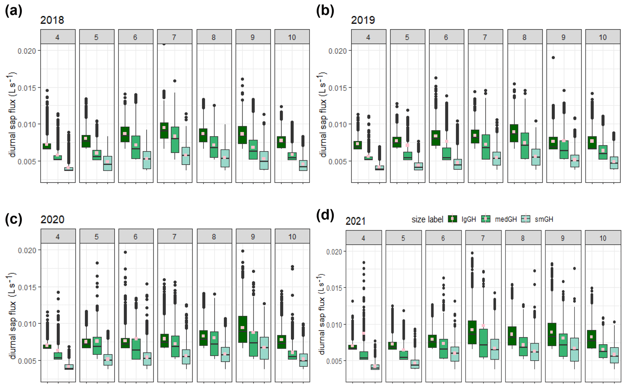
Figure 2 Comparison of diurnal sap flux measured by each probe set for three (small (smGH), medium (medGH), and large (lgGH)) ghost (no-infrastructure, no-control) trees in the years 2018–2021 (panels (a), (b), (c), and (d), respectively) across the treatment season, April–October (numbered subpanels within panels a–d). Monthly 95th percentile values are shown separately (Fig. S5 in the Supplement). The graphical display is cropped at a sap flux of 0.02 L s⁻¹. Mean values, calculated from the entire range of data, are shown as spots (pink).

Interquartile ranges are generally larger in the middle of the growing season for all sizes of example trees and collapse towards the minimum detectable value for each tree size at either end of the growing season. The minimum detectable sap flux using the present method is tree-size dependent (Appendix A, Table A2, stage 5): 0.0035 L s⁻¹ (3.5 mL s⁻¹) for the smallest tree in Fig. 2, 5.2 mL s⁻¹ for the medium-sized tree, and 6.5 mL s⁻¹ for the largest tree shown. The imbalance between the probe set data on the example trees (Fig. 2) can be up to ± 25 % (Fig. S4). This is greater in the earlier years, 2017 and 2018. This imbalance determines the spread of the IQR when normalised tree values are combined. All the large-tree-example sap flux values lie within a factor of 3 of the minimum detectable value (i.e. to 0.02 L s⁻¹) until June 2020 (more than 4 years after installation), after which larger extreme values are present.

The distributions of the three examples are clearly offset by tree stem size, suggesting that normalisation by size may be useful for inter-tree and array-to-array comparison (Sect. 3.3). For these example trees, mean monthly diurnal sap flux increased in the spring from first leaf (see phenology in Table 1 above) to achieve peak values in July in 2018 and 2021. In 2019 and 2020, increases in mean monthly diurnal sap flux were more gradual throughout the treatment season, reaching peak values in August (2019) and September (2020). There was then a faster decrease in sap flux until end of October (the end of the CO₂ treatment season) or later, presumably due to leaf senescence and the shortening of day length.

It is evident that there are highly skewed distributions in Fig. 2. Figure S5 reports 95th percentile sap flux values for each probe set and month across 2017–2021, showing variability in the timing of the highest monthly 95th percentile sap flux of the half-tree data for each tree across the years of study. The 95th percentile sap flux is not synchronised for all probe sets on a monthly basis, indicating the dominant role of individual tree characteristics or position in determining sap flux extrema (Dragoni et al., 2009). Although minimised as much as practicable (see Sect. 2.6 above), such individual characteristics cannot be completely eliminated and may relate to major changes in branch structure (e.g. from wind damage or mortality) affecting canopy photosynthetic controls. They may also depend on the aspect of the tree and competition for root water (proximity to other trees), indicating seasonal influences on leaf, branch, and root growth.

3.2 Diurnal TWU variation between trees

3.2.1 TWU as a function of stem radius

Example relationships between R_b (mm) and monthly mean TWU ($\stackrel{\mathrm{‾}}{\mathrm{TWU}}$, L d⁻¹) for all trees with both probe sets working were first analysed for the 2019 summer months. July was used for comparison, as typically it exhibits maximum $\stackrel{\mathrm{‾}}{\mathrm{TWU}}$. The hypothesis that $\stackrel{\mathrm{‾}}{\mathrm{TWU}}$ is a function of R_b was tested by a simple regression model. The best fit model for the combined 2019 data across all treatments was a simple linear fit; quadratic fits were tested and rejected. During July 2019 due to two probe sets malfunctioning, ghost tree $\stackrel{\mathrm{‾}}{\mathrm{TWU}}$ results did not include trees as large as the largest in the infrastructure arrays, as explained in the Methods above. Data from 6, 13, 17, and 17 trees were used for the years 2018, 2019, 2020, and 2021, respectively.

Data for July of the years 2017–2021 are shown in Fig. 3, illustrating the differences by year (Table 2) and treatment. The shorter regression for the ghost array trees (Fig. 3a and b) has a smaller slope than infrastructure (eCO₂ and aCO₂) array trees that exhibit similar slopes. Table 2 lists July model slopes for the years 2018–2021 for all treatments combined. The slopes are within +20 % and −30 %, giving a mean slope of 3.1±0.4 L d⁻¹ mm⁻¹ for 274 mm $\le R_b\le \mathrm{465}$ mm, although the steepest slope (July 2018) and the shallowest slope (July 2020) differ by more than their combined standard errors and so may represent different relationships. The intercept of the linear regression is not physically meaningful, as we are only considering a relationship for trees of R_b between 0.25 and 0.5 m. The results confirm the recent study by Schoppach et al. (2021) (and supporting reference Hassler et al., 2018) with respect to the relationship between diameter at breast height (DBH; ∼ 1.3 m above the ground surface) and the water usage of oak.

Table 2 Linear regression model parameters for July mean TWU ($\stackrel{\mathrm{‾}}{\mathrm{TWU}}$, L d⁻¹) versus the stem radius at insertion point (R_b, mm). August 2019 is also shown. The final row shows model statistics for all months of July in the years 2017–2021 for 55 trees. The table does not discriminate $\stackrel{\mathrm{‾}}{\mathrm{TWU}}$ with respect to treatment. See Appendix A, Table A1 for statistical abbreviations.

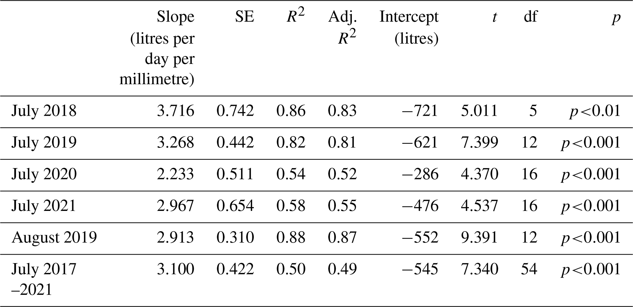
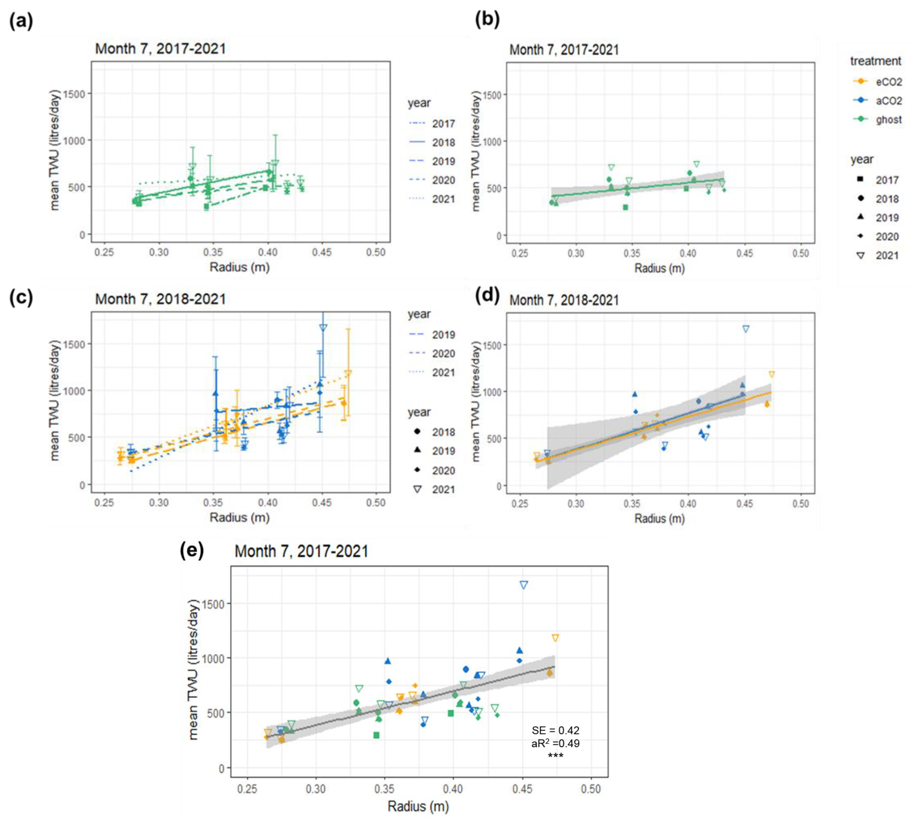
Figure 3 Mean July TWU ($\stackrel{\mathrm{‾}}{\mathrm{TWU}}$ L d⁻¹) versus stem radius R_b (m) at measurement height is shown for the three treatment types in the years 2017–2021. Panels (a) and (b) show ghost (no-infrastructure, no-treatment) trees in all years. Panels (c) and (d) show infrastructure arrays for treatment (eCO₂) and infrastructure control (aCO₂) for the years 2018–2021. Panels (b) and (d) show treatment regression lines for all years combined. Panel (e) shows points for all years with a single regression line. R_b is linearly proportional to $\stackrel{\mathrm{‾}}{\mathrm{TWU}}$ (mean slope 3.1±0.4 L d⁻¹ mm⁻¹). The error bars in panels (a) and (c) show SD. Panel (e) additionally shows significance (${}^{***}$ p<0.001), SE, and the adjusted R² (aR²) values.

The slopes of the three treatments for July data in all years were also compared to determine the differences due to treatment (Table S5). There is a 10 % difference between infrastructure treatment tree slopes (Table S5 and Fig. 3d; aCO₂ slope = 3.86, SE = 1.25 L d⁻¹ mm⁻¹. eCO₂ slope = 3.55, SE = 0.31 L d⁻¹ mm⁻¹), which is not statistically significant given the standard error of the slopes. Overall, for infrastructure treatment trees (eCO₂ and aCO₂; Fig. 3d), the slope is greater than for no-infrastructure ghost array trees (slope = 1.2, SE = 0.47 L d⁻¹ mm⁻¹) (Fig. 3b), and the magnitude of $\stackrel{\mathrm{‾}}{\mathrm{TWU}}$ for all infrastructure trees is greater for a given size.

3.2.2 Factors affecting $\stackrel{\mathrm{‾}}{\mathrm{TWU}}$ as a function of R_b

The relationship with $\stackrel{\mathrm{‾}}{\mathrm{TWU}}$ varies on a year-to-year basis between 2.2 and 3.7 L d⁻¹ mm⁻¹ of R_b. This is due, in years of lower values, to relatively larger decreases in $\stackrel{\mathrm{‾}}{\mathrm{TWU}}$ of large trees compared to that of the smaller trees in the sample. Oaks respond subdaily to solar radiation reduction events (Fig. S9) during cloud cover, suggesting that the year-to-year differences in slope (Table 2) are affected primarily by environmental factors (Wehr et al., 2017). In July 2020, the wettest year for mid-leaf (see Table S14 and Figs. S14 and S16), we are not able to distinguish whether the smaller slope arises from (a) smaller-tree $\stackrel{\mathrm{‾}}{\mathrm{TWU}}$ being enhanced due to the truncation effect (Appendix B), (b) larger-tree $\stackrel{\mathrm{‾}}{\mathrm{TWU}}$ being suppressed under poor light levels relatively more than the smaller trees, or (c) a combination of these two factors. Nonetheless, the inter-year variation in the regression is likely due to monthly weather variation, such as different numbers of days of full sunlight or more days of rain (Table S14 and Fig. S16).

3.2.3 Canopy area, A_c, as a function of stem radius, R_b

Canopy area, A_c (m²), measured in the year of installation (first) and in early 2022 (last), correlates closely with R_b (Fig. 4 and Table 3, also Table S6 for data concerning repeat measures for each tree). On average, A_c is linearly proportional to R_b (∼ 617±108 m² m⁻¹; 0.261 m ≤ R_b≤ 0.473 m). There are changes in A_c (some positive and some negative) between the first and last measurements.

Table 3 Oak tree canopy area A_c (m²) versus stem radius (m) at the insertion point. Data from 18 trees for two (first, last) A_c measurements are shown (fourth row) and modelled by treatment (rows one to three). The first readings were taken soon after installation; the last readings were done in early 2022.

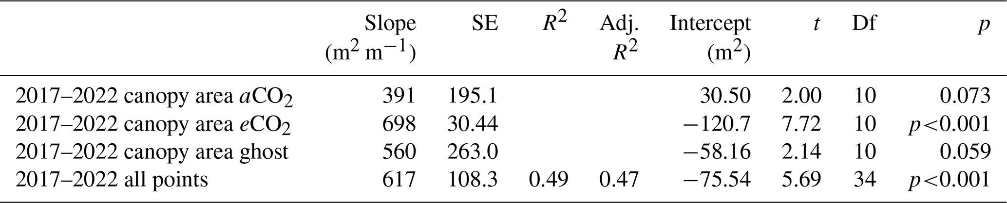
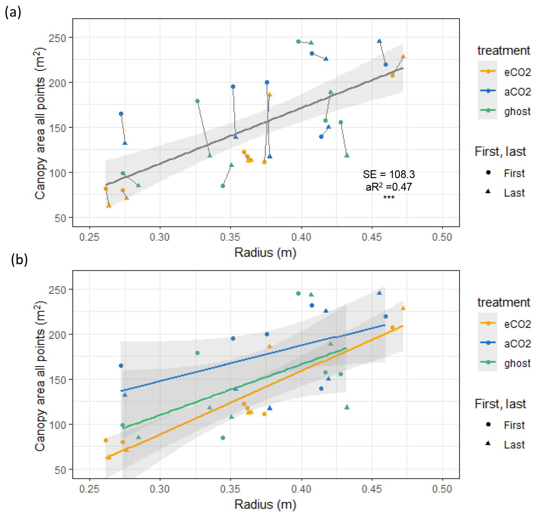
Figure 4 Canopy area A_c (m²) variation with stem radius R_b (m) for target oak trees measured in the dormant season on two occasions per tree. Significance values, SE, adjusted R² (aR²), and slopes are shown in Table 3. The first measurement year is 2017–2018. The last measurement year is 2022. Panel (a) shows a linear model for all trees monitored, showing the significance ($***$ signifies p<0.001), SE, and aR² values. A_c is linearly proportional to R_b (∼ 617 ± 108 m² m⁻¹; 0.261 m $\le R_b\le \mathrm{0.473}$ m). A line joins the first and last measurements. Panel (b) shows linear model relationships by treatment. Error bars show SD.

The three treatments do not show statistically significant differences in A_c per unit tree radius; eCO₂ has the greatest A_c per R_b, but the other fits, although smaller in the mean slope, fitted much worse to the linear model, resulting in much larger standard errors of the mean slope (Table 3, second column).

The measurements of A_c taken here are useful to assess water usage per unit of projected area of plant canopy but are insufficiently precise to quantify treatment effects. Changes in A_c, presumably due to a combination of measurement uncertainties and other influences, such as branch growth or loss during severe wind events, do not impact the significance of the overall A_c versus R_b relationship (Table 3, all points).

We could use either R_b or A_c to remove the tree size dependence of sap flux (Fig. 2) and hence $\stackrel{\mathrm{‾}}{\mathrm{TWU}}$, exemplified in Fig. 3 above. Using the overall regressions in Tables 2 and 3, along with measurement error, the average July diurnal water usage is 5±0.3 L d⁻¹ m⁻² (A_c). We use R_b (Fig. 5) below as the more convenient normalising factor (as it can be measured manually more easily and accurately by forest practitioners).

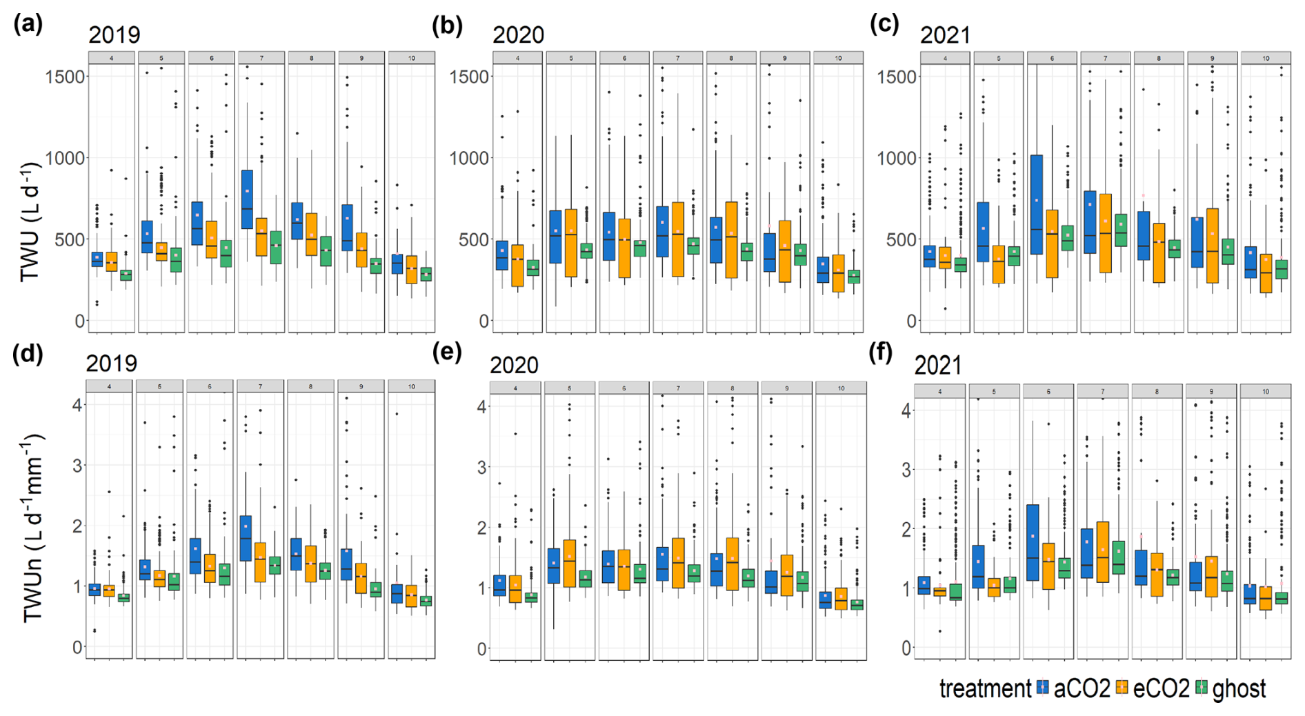
Figure 5 Treatment comparison of TWU. For the years 2019–2021, the TWU data are shown for the three treatment types. Tree data are combined for each treatment month from April to October. The distributions are shown as box and whisker plots showing the median and interquartile range (IQR, 25th percentile to 75th percentile), with whiskers calculated as 1.5 × IQR from the hinge and points for outliers. Mean values, calculated from the entire range of data, are shown as spots (pink). Panels (a), (b), and (c) show TWU (L d⁻¹) for the years 2019, 2020, and 2021. Panels (d), (e), and (f) show TWU_n (L d⁻¹ mm⁻¹), i.e. TWU normalised by the stem radius (mm) at the stem probe insertion height.

3.3 Yearly and seasonal variation in TWU

Box and whisker plots show TWU (Fig. 5a, b, and c) for the years 2019–2021 and treatments across the treatment season (April–October). In comparison, TWU normalised by individual-tree bark stem radius Rb, which we will call TWU_n (L d⁻¹, mm⁻¹), is shown for the same years in Fig. 5d, e, and f. The years 2017 and 2018 are omitted because they have a smaller number of data points (Fig. S6) and are not fully representative of the tree size range across treatments.

For the years 2019–2021 (Fig. 5a, b, c), mean, median, and 75th percentile TWUs (L d⁻¹) increase steadily with day length and solar radiation (Fig. S11) from around budburst (April/May) to a broad summer maximum (June, July, August) and then decline with day length to full-leaf senescence (October–November). Similar patterns are exhibited during 2017 and 2018 (Fig. S6).

In comparison, TWU_n exhibits lower within-month variability, indicated by smaller interquartile ranges, although the basic relationship between treatments remains (Fig. 5d, e and f). There is close correspondence between TWU and TWU_n inter-year patterns for all three treatments across the leaf-on seasons. The starting levels in April (lowest in 2019) and the peak month (July or August) of median TWU_n vary year on year, likely resulting from differing throughfall and soil moisture retention within the previous 12 months (Supplement Appendix S-A). Figure S7 shows the monthly sap flux and TWU_n 95th percentiles for all trees, illustrating the variation in high value extrema.

3.4 Statistical testing of hypotheses

Using summary statistics (a traditional method for repeated-measure analysis) for each individual (e.g. the mean of TWU_n ($\stackrel{\mathrm{‾}}{{\mathrm{TWU}}_{\mathrm{n}}}$)) on a monthly and an annual-treatment-season basis, with ANOVA and equivalent nonparametric tests, inter-year and seasonal trends were identified. Initially, variance of tree water usage was tested using normalised data (TWU_n) per tree grouped by treatment type. The ANOVA results, before consideration of residuals, are outlined in the Supplement (Fig. S8, Tables S7 and S8). Mean values for TWU_n ($\stackrel{\mathrm{‾}}{{\mathrm{TWU}}_{\mathrm{n}}}$) in the treatment season and in July for each of the years from 2019 to 2021 were calculated and compared. Levene's test was applied, showing the heterogeneity of variance of TWU_n data for each model using both the median and the mean. The results are reported in Table S9 for the infrastructure groups (eCO₂ and aCO₂) and Table S10 for the control groups (aCO₂ and ghost). Additional analyses were undertaken: ANOVA using the natural logarithm transform and the nonparametric Wilcoxon ranked-sum test. Both produced very similar results to the initial ANOVAs, and corrections were considered for application to reflect the repeat use of aCO₂ data, but these do not enable a full assessment of the repeated measures concerning the trees and time.

3.4.1 Models for repeated-measure nonlinear data

TWU_n data for each whole season of interest were next modelled using GLMMs for each season of interest (2019, 2020, 2021). The intention was to develop a simple and parsimonious model sufficient to test the hypotheses outlined in Sect. 1. Before modelling, some tree TWU_n data were removed from each season data model where more than half of the days were missing from the season (see Table S11).

To test hypothesis 1, infrastructure tree TWU_n data (eCO₂ and aCO₂) for each CO₂ season of interest (2019, 2020, 2021) were analysed using gamma GLMM models with a log link. A random-intercept model structure was adopted, incorporating random components for each tree (tree label) and for time (DOY): TWU_n ∼ CO₂ + (1 | DOY) + (1 | tree label). We tried other model structures, i.e. just the array and a nested array–tree as random elements, but using the Akaike information criterion (AIC) and Bayesian information criterion (BIC) from the anova function in R for model comparison, we selected the above as the best model. Figure 6 and the associated Table 4 show the results of these repeated-measure models for eCO₂. Complete model statistics are tabulated in Table S12 in the Supplement.

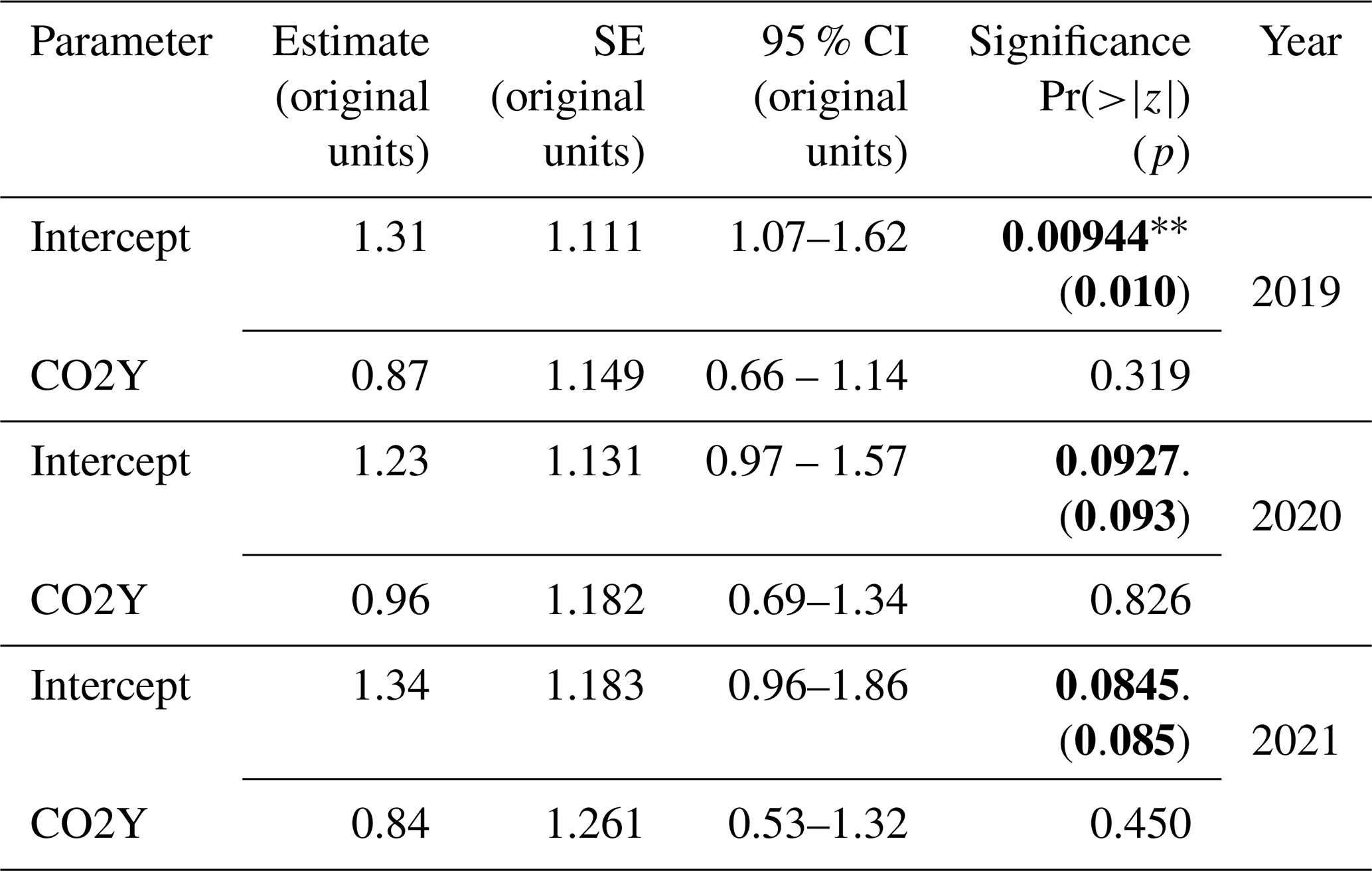
Table 4 Hypothesis 1 – CO₂ effects. GLMM random-intercept model outputs for (eCO₂ : aCO₂) TWU_n for each year from 2019 to 2021, inclusive. The estimate, SE, 95 % CI, and significance are shown. Significance values Pr($\mathit{>}\left|z\right|$) are taken from summary outputs. All other results (including p) are from tab_model outputs in the original data units for TWU_n (L d⁻¹ mm⁻¹). Bold typeface indicates a p value <0.1.

Significance categories are ${}^{***}<\mathrm{0.001}$, ${}^{**}<\mathrm{0.01}$, ${}^{*}<\mathrm{0.05}$, and $\mathrm{`}\mathrm{`}{.}^{\prime \prime }<\mathrm{0.1}$. The 1 is included to show no significance category (between 0.1 and 1), and the zero is the boundary point for ${}^{***}$ (between 0 and 0.001).

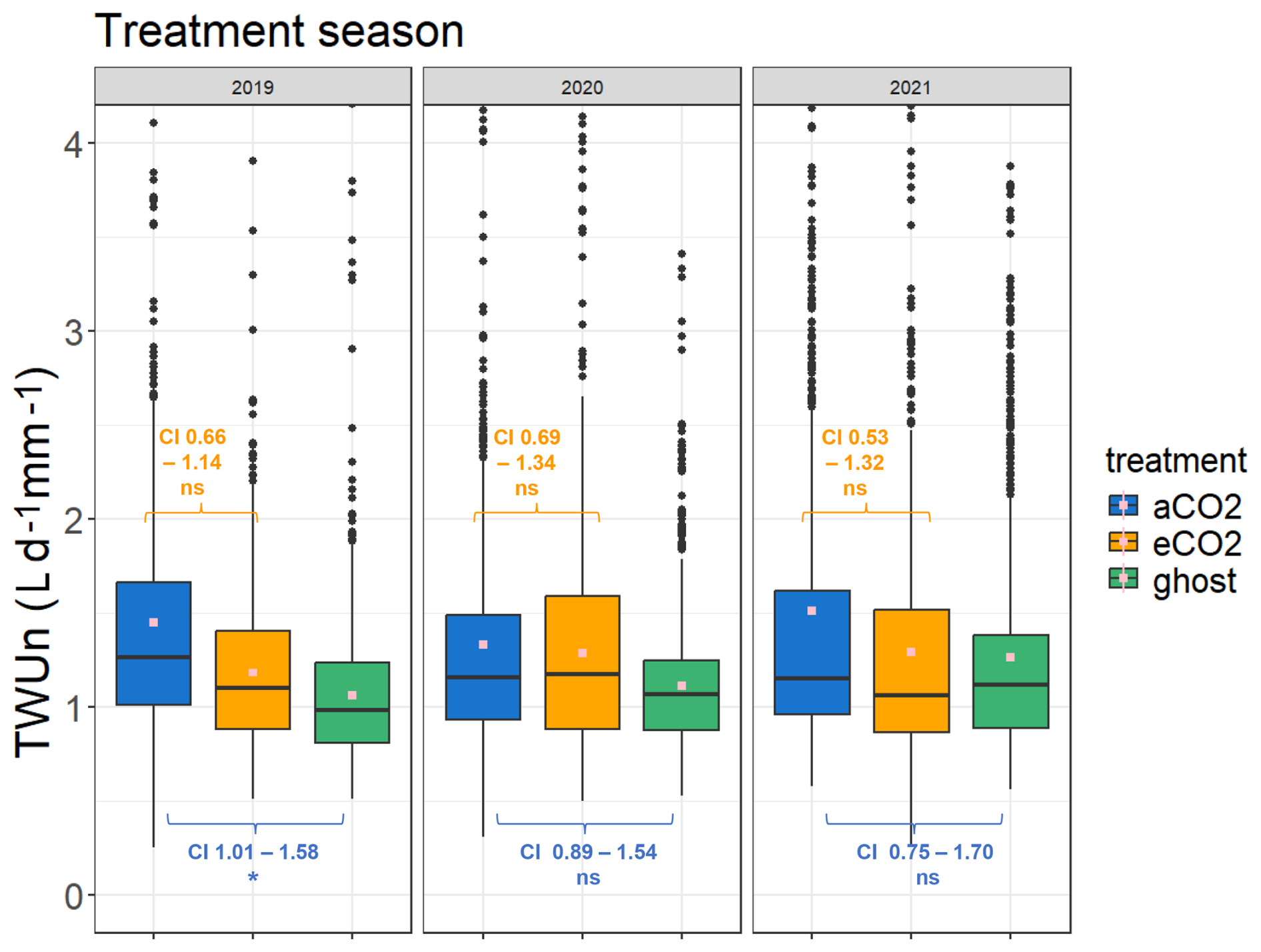
Figure 6 Treatment comparison of TWU_n (L d⁻¹ mm⁻¹) for the years 2019–2021. The April–October inclusive season data are combined for each year. The TWU_n y-axis scale is truncated for clarity, with small numbers of additional outliers. Maximum TWU_n values for each distribution each year (reading from left to right) are 8.0, 3.9, 4.2, 6.6, 4.1, 4.8, 6.6, 8.0, and 4.8 L d⁻¹ mm⁻¹. The whole-season mean values are shown in pink. The 95 % confidence intervals (CI) of the treatment effects from the GLMMs are indicated in orange (hypothesis 1, Table 4) for the eCO₂ : aCO₂ model and blue (hypothesis 2, Table 5) for aCO₂ : ghost model. Values for the treatment season TWU_n in each year are given. One-way ANOVA results are shown in Fig. S8a and b and Tables S7 and S8.

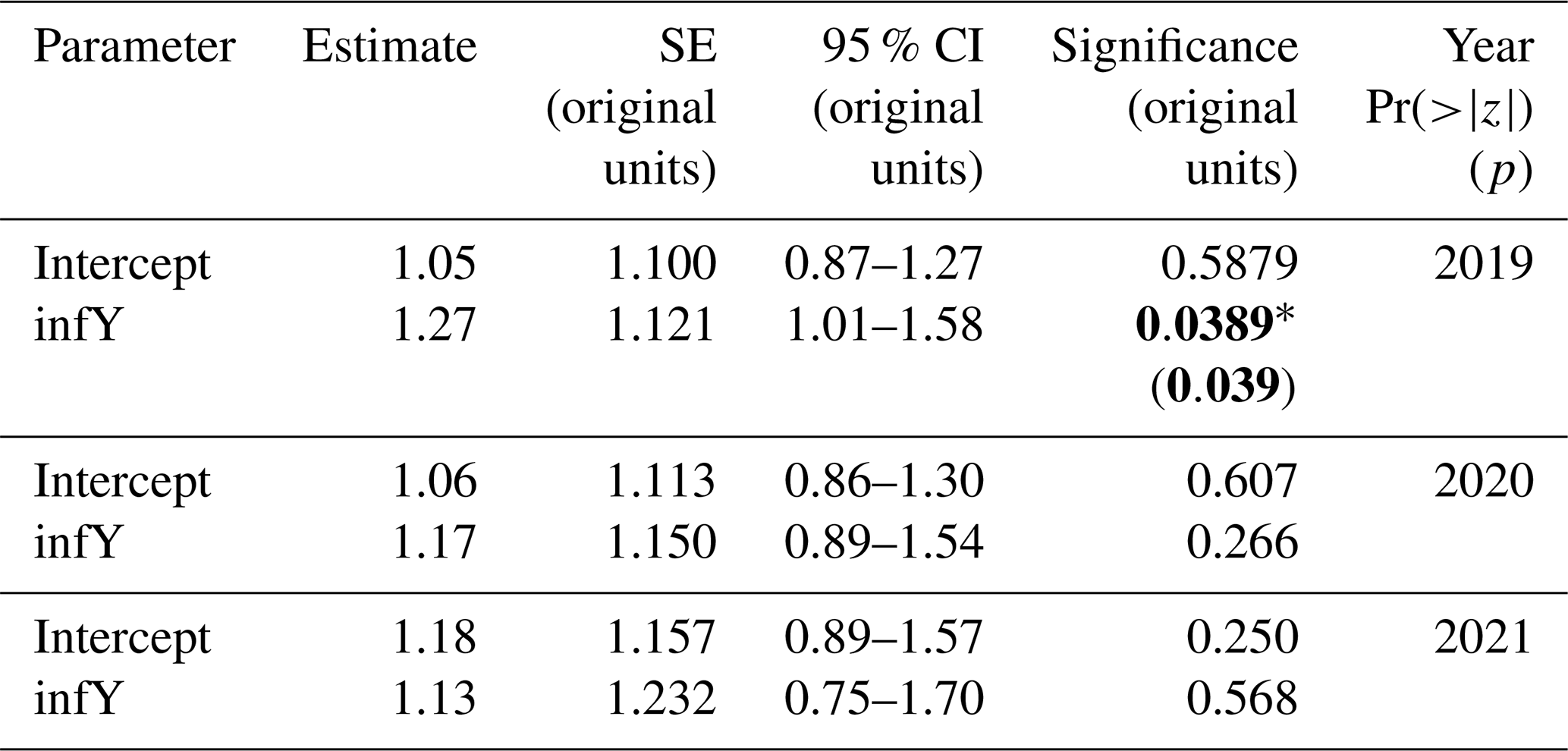
To test the hypothesis 2 control group, tree data (aCO₂ and ghost) were analysed for infrastructure (inf) effects using the same the treatment seasons (2019, 2020, 2021) and similar random-intercept models: TWU_n ∼ inf + (1 | DOY) + (1 | tree label). Figure 6 and the associated Table 5 show the results of these repeated-measure models for infrastructure. Complete model statistics are tabulated in Table S13 in the Supplement.

Table 5 Hypothesis 2 – infrastructure effects. Random-intercept GLMM outputs for (aCO₂ : ghost) TWU_n for each year from 2019 to 2021, inclusive. The estimate, SE, 95 % CI, and significance are shown. Significance values Pr($\mathit{>}\left|z\right|$) are taken from summary outputs. All other results (including p) are from tab_model outputs in the original data units for TWU_n (L d⁻¹ mm⁻¹). Bold typeface indicates a p value < 0.1.

Significance categories are ${}^{***}<\mathrm{0.001}$, ${}^{**}<\mathrm{0.01}$, ${}^{*}<\mathrm{0.05}$, and $\mathrm{`}\mathrm{`}{.}^{\prime \prime }<\mathrm{0.1}$. The 1 is included to show no significance category (between 0.1 and 1), and the zero is the boundary point for ${}^{***}$ (between 0 and 0.001).

4 Discussion

Mean normalised water usage, $\stackrel{\mathrm{‾}}{{\mathrm{TWU}}_{\mathrm{n}}}$, ANOVAs are suitable for initial testing of treatment hypotheses, as they use accumulated daily data and mean values across longer periods (months, years). These analyses align with techniques previously used for FACE experiments, extending those from previous eCO₂ studies of oak (e.g. Leuzinger and Körner, 2007) by being over of a longer duration of treatment (numbers of years and numbers of treatment days per year) and a greater size range and sample of trees. A more robust approach to account for random repeated-measure effects (individual and time) uses generalised linear mixed-effect model (GLMM) analysis. Findings from ANOVA and GLMM are discussed below versus each of the paired treatment comparisons undertaken.

4.1 TWU_n differences under eCO₂

Table 4 reports reductions in eCO₂ TWU_n compared to aCO₂ TWU_n (for the ANOVA model results; see Fig. S8 and Table S7 in the Supplement). Across whole growing seasons, the estimated (converted to a percentage) fixed-effect reduction from the GLMM in 2019 is 13 %. In 2021 a 16 % reduction is seen, whereas in 2020 only a 4 % reduction is shown. The model accounts for the individual and time-related repeated measures, but in all years these affects are low, supporting our original ANOVA model results. These models confirm our hypothesis 1, i.e. that there is likely to be reduced tree water usage over whole seasons. We also observe substantial interannual variability in fixed effects. This implies we cannot yet obtain a definitive prediction of the mean amount of TWU_n reduction per annum as a fixed effect of eCO₂. A greater number of years of results, given the changes in long-term trends of, for example, precipitation, would be necessary to detect any long-term trend. July-only results have not been adjusted for repeated measures and are less conclusive than the traditional ANOVA analyses (Table S7).

We are not aware of other whole-growing-season oak results with which to compare these TWU_n results. Each treatment TWU_n is a proxy for stand transpiration, so we next compare our FACE results to eCO₂ : control transpiration ratios from previous FACE experiments of oak and other deciduous species.

Short-duration midsummer FACE results have been reported for mature temperate broadleaves. Leuzinger and Körner (2007) were unable to statistically test species-specific differences in transpiration for adult Q. petraea (Matt.) Liebl. under eCO₂ in their Web-FACE experiment but found a 14 % reduction overall when results for Q. petraea were pooled with those of Carpinus betulus L., and Fagus sylvatica L. in the summers of 2004 and 2005. Their Web-FACE operated under a similar CO₂ elevation (ambient is not reported) to that used at BIFoR FACE. Our uncorrected July-only TWU_n results (reductions in every year but likely to be significant only for the uncorrected 26 % reduction in 2019) for Q. robur differ from their results for Q. petraea but strengthen their overall conclusions regarding adult deciduous broadleaves and regarding the large interannual variability they also observe.

Both seasonal and summer results at Oak Ridge National Laboratory (ORNL) are reported by Warren et al. (2011a) for 11-, 16-, and 20-year-old Liquidambar styraciflua L. in the years 1999, 2004, and 2008 and in the early 2007 season by Warren et al. (2011b). Again, a similar FACE CO₂ elevation was used as at BIFoR FACE. ORNL ambient CO₂ levels were 380–400 µ mol mol⁻¹, giving a ∼ 40 % elevation compared to our current ∼ 35 %. Warren et al. (2011a, their Table III) report 10 %–16 % seasonal reductions in stand transpiration under eCO₂, which increased with the year of treatment. This may reflect a differing species response to eCO₂. For summer only, a 7 %–16 % reduction was reported, whilst Warren et al. (2011b, their Fig. 1) report ∼ 28 % reductions in the (non-drought) first half of a single growing season at the same ORNL site. This again reflects large interannual summer response variability.

The reductions in TWU_n in our study are consistent with other treatment effects seen at BIFoR FACE: diurnal results for photosynthetic enhancement (23 ± 4 % higher for eCO₂, Gardner et al., 2022, although not specifically targeted at the focal TWU_n trees), and fine root production (45 % higher for eCO₂ in the first 2 years (Ziegler et al., 2023) covering the whole year rather than the season only). Synthesis of these treatment effects into quantitative budgets for water and carbon is outside the scope of the present work.

4.2 FACE infrastructure effect on TWU_n

The effect of FACE infrastructure on tree water usage has, to our knowledge, not been previously reported. TWU_n was higher for the infrastructure control aCO₂ trees compared to ghost (i.e. no-infrastructure) trees across the 3 treatment years analysed, 2019–2021. In the 2019, 2020, and 2021 seasons, the ANOVA models (Fig. S8, Table S8) found a consistently significant 37 % to 20 % increase in mean aCO₂ TWU_n compared with ghost TWU_n. In contrast, the GLMMs showed a significant fixed effect only in 2019 (Fig. 4, Table 5), estimated to be a 27 % increase under infrastructure conditions. In 2020 and 2021, the models showed nonsignificant fixed effect increases of 17 % and 13 %. These tests confirm our hypothesis 2 that there is increased water usage within FACE infrastructure treatments but do not yet enable us to predict the amounts in any given year due to the environmental interannual variations.

The results of this study indicate the importance of infrastructure controls in forest FACE experiments. The greater aCO₂ TWU_n may be due to one or more of several factors: the effects of FACE infrastructure gas injection on air mixing and turbulence and hence changes in microclimate; differences in ground cover; or array-specific differences in soil moisture, slope, soil respiration, or the species of subdominant trees present. Further work is needed to fully explore these results.

Since the treatment effect for eCO₂ has the opposite sign to that for infrastructure (i.e. we see a reduction in eCO₂ TWU_n compared with aCO₂ TWU_n but an increase in aCO₂ TWU_n compared with ghost TWU_n), the infrastructure treatment effect cannot cause a pseudo-eCO₂ effect in the statistics, but it does further reduce any certainty about the absolute magnitude of the eCO₂ effect.

4.3 Capabilities, limitations, and usability of sap flux data from HPC probe sets

Although this experiment had a relatively small sample size (a total of 18 trees, with 6 per treatment), it was nevertheless a substantive experiment consisting of 12 259 d of individual tree data (770 667 diurnal sap flux measurements) in a unique experimental setting, making this dataset of high value for modellers of dynamic vegetation, water, and climate. We have defined a parameter TWU_n to enable consistent water usage comparisons between individual trees and hence treatments diurnally across both summer months and whole seasons. We believe that this method of processing HPC sap flux results, along with the extensive and continuous dataset for all no-infrastructure ghost control trees over more than 4 years, provides high confidence in this normalised data.

We can clearly demonstrate that the use of four thermocouple positions across the sapwood for each of our HPC probe sets has enabled us to successfully capture the position and size of point sap flux density (derived from sap velocity) and that this has given us a more reliable basis to explore the effects of tree size on both whole-probe-set sap flux and TWU. With respect to sap flux, single-probe sets are unlikely to provide representative results of TWU due to asymmetry in sapwood radial width around the circumference of the tree. The effects of the time-out value in the HPC measurement system have been discussed (Appendix B), and recommendations are made to ensure that any repeat experiments using this technique consider truncation effects for diurnal sap flux.

5 Conclusions

Water usage was calculated from stem sap flux for 18 oaks in an old-growth even-aged plantation during the first 5 years of an eCO₂ treatment. The oaks were distributed across the three treatment conditions: eCO₂, aCO₂, and ghost. Diurnal (i.e. daylight) responses that accumulated over days, months, and growing seasons (April–October, inclusive) were the focus. Within a given year, median, mean, and extreme (95th percentile) diurnal sap flux increased in the spring from first leaf to achieve peak daily values in summer months (July, August). We aggregated sap flux daily to derive water usage information for each tree, averaging results from two probe sets per tree to eliminate orientation imbalances.

Differences in tree water usage varied according to tree size. Tree characteristics, R_b and A_c, were measured and correlated linearly with mean diurnal water usage, $\stackrel{\mathrm{‾}}{\mathrm{TWU}}$, for July, confirming a recent study (Schoppach et al., 2021). The linear relationship between A_c and $\stackrel{\mathrm{‾}}{\mathrm{TWU}}$ is less certain than that between R_b and $\stackrel{\mathrm{‾}}{\mathrm{TWU}}$ but can be used to convert tree-based transpiration to a stand scale (Granier et al., 2000) for comparison with dynamic vegetation and climate models.

Normalisation of TWU by R_b to give TWU_n enabled comparison of data combined from multiple trees across the treatments. A growing-season reduction in TWU_n under eCO₂ was detected; the signal was less clear for July-only data. Repeated measures due to individual trees and time affected the response but did not dominate the perceived effects when modelled. There was considerable interannual variability in the treatment effect for growing-season and July-only averages, likely related to environmental drivers, but which remains to be diagnosed or modelled fully.

Growing-season and July-only increases in TWU_n under aCO₂ compared to non-infrastructure controls (ghost trees) were detected consistently in ANOVA in all years, whilst the repeated-measure GLMMs estimated significant effects only in the 2019 season (and reduced the percentages by up to a third in all seasons in comparison to ANOVA). This shows that either the presence of infrastructure affects water usage or the ghost positions are not comparable to those of the infrastructure arrays due to array-specific differences in soil moisture, slope, soil respiration, or the presence of subdominant tree species.

Whilst the experiment produced reliable data across the 5 years, outlier incidence appears to be increasing, and re-installation of probe sets is recommended. To detect cavitation and embolism in situ as a possible cause of outlier data, separate (e.g. acoustic) monitoring would be required. Whilst much further work remains, this first set of tree water usage results strongly supports the conclusion that old-growth oak forests conserve water under eCO₂ at the whole-plant level.

Appendix A: Additional tables

Table A1 Table of parameter symbols and statistical abbreviations.

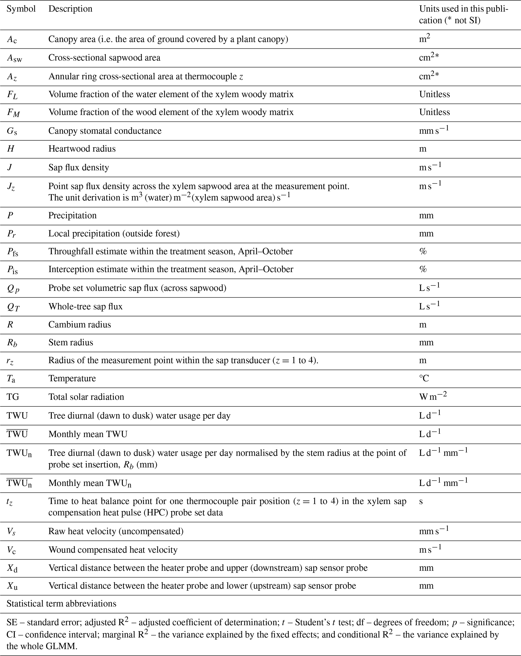
Table A2 Calculations of stages 1 to 7 showing the flow of data processing to obtain TWU from time to heat balance t_z from all differential HPC probe set thermocouple radial positions.

Appendix B: Limitations of the time-out characteristic and outliers

There are known limitations in the ability of the HPC system to measure low and reverse sap velocities (Forster, 2017) and to some extent high sap velocities (Burgess et al., 2001). With respect to our setup, we optimised the high end of this limitation. The sap probe manufacturer Tranzflo has extensive experience in a wide range of deciduous trees. The probe sets used were custom-made for us to suit oak trees of this size, using sensor spacings suggested by Tranzflo. The limitations of the time-out characteristic and the effect this places on HPC data are recorded in several references (e.g. see Tranzflo, Measurements of Sap Flow by the Heat-Pulse Method. An Instruction Manual for the HPV system, 2016). The limitations impact our choice of data processing (e.g. diurnal versus diel) and feed through into the statistics we report. These limitations also introduce a truncation effect at lower heat velocities such that the distribution of the resulting raw and processed data is not symmetrical. We had limited options to extend the time-out period due to the multiple types of data that we needed to capture with our single logger–multiplexer arrangement in each array.

To normalise the data, given the above time-out effect, we select only those daylight periods where we can be confident that all four thermocouples are measuring and where they exhibit a shaped maximum point sap flux density value. We also focus on accumulation and percentile ranges rather than point time results. It is possible to use fewer positions for our calculations if, for example, one probe set position is giving a constant truncated value. These instances would need individual verification.

There were limited options to extend the time-out period for the combination of Tranzflo probe set system and Campbell Scientific logger–multiplexer used in this project. Based on our experience, extending the time out beyond double (i.e. beyond 660 s = 11 min) would be impractical for the current setup. Extension beyond, say, 7 min (420 s) would likely require a decrease in the sampling frequency to 1 s (currently set to 0.5 s) to ensure that sufficient memory is available during the differential calculation period. This decrease in sampling frequency is an inevitable compromise between capturing low heat velocities and offering sufficient data discrimination to capture the variation in heat velocity towards the maxima of the daily cycle.

Appendix C: Details of xylem sap flow measurements and calculations

In each research array, a data logger and multiplexer (CR1000 and AM25T, Campbell Scientific, Logan, Utah, USA) were used for year-round 24 h capture of raw data from sap flux HPC probe sets manufactured by Tranzflo (New Zealand) soil and throughfall measurement devices.

The logger was programmed for data capture using CRBasicEditor under LoggerNet (versions up to 4.6.2), also by Campbell Scientific, Logan, Utah, USA. We tested our prototype installation setup in midsummer 2017 to determine whether we could capture the expected range of heat velocities and applied similar capture programs to all array loggers.

Each target oak tree had two probe sets, east and west facing, using long (7 cm four-sensor) probes. Each probe set was inserted at a stem height between 1.1 and 1.3 m and contained a central heat pulse probe and two measurement probes (with each long probe containing four thermocouples) upstream and downstream of the heater (Fig. S2). Transducers were positioned radially in the stem (to suit the ring-porous characteristics and bark thickness of these Q. robur trees). Each probe set was protected from natural heating by reflective insulation covers during the treatment season.

During monitoring, a heater pulse of 1.5–2.5 s in duration was applied half-hourly through a heater box (one per tree) to the heater probes. The pulse duration was dependent on the number of heaters pulsed simultaneously. A 2 s pulse was standard for the two oak trees per array (four long probe set) configuration. Each thermocouple pair in the upstream and downstream positions took up to 330 s (5.5 min) to reach a differential heat balance point, and this time determined the minimum detectable heat velocity for a time just within this time-out period. The thermocouple data logger sampling rate of 0.5 s determined the maximum detectable speed (minimum time to balance), which, given normal interference levels, was adequate for deriving the maximum heat velocity. A total of 16 differential thermocouple configurations were sampled per array in one 6 min time slot every 30 min, giving time-to-balance t_z data in seconds.

Data collection problems, due to logger grounding and sap probe disconnections at manufacture, caused data loss early in the project. Contact with sapwood was maintained for all oak trees from installation to March 2021, when 2 out of the 36 probe sets failed.

C1 Raw file processing

Logger data from the nine C1000 FACE research loggers were collated by array and transducer type (i.e. 7 cm probe set datasets for oaks only) using R and then combined into year files for further data processing.

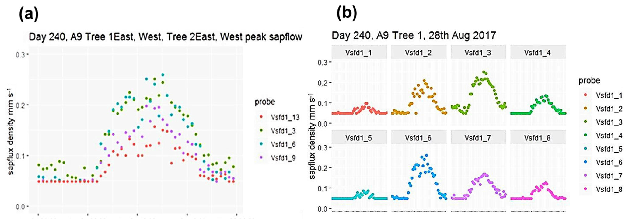
Figure C1 (a) Example (DOY 240) of the stage 4 output showing peak point sap flux density in two trees for a sunny day in August 2017. The tree 1 (vsfd1_3 and vsfd1_6) stem radius is larger than that of tree 2 (vsfd1_9 and vsfd1_13). (b) Example (DOY 240) of the stage 4 output showing changes to point sap flux density across the active xylem for east-facing (top) and west-facing (bottom) probe sets of one tree (tree 1) on the same day in August 2017. The left-hand probe position is nearest to the bark, and the right-hand probe position is nearest to the heartwood. Note that the peak value occurs at different sensor positions for the two probe sets.

C2 Xylem sap flux calculations

Following quality checks, each stage of calculation to produce wound-corrected sap velocity and sap flux density at each transducer position (four per probe set) was performed in stages (see Table A2). Table A2 lists the methodology and equations, along with the associated literature sources for each stage.

At stage 3 (Table A2), the Green and Clothier (1988) polynomial factors were used for wound compensation. For stage 4, the conversion factor c1 was derived from measurement of wet and dry wood cores and micro-cores (Eqs. A4 and A5) to calculate xylem sap velocity from heat velocity in oak wood.

Short incremental wood cores (∼10 cm long, 4 mm diameter) were taken from two oaks outside of the experimental arrays. Micro-cores were also taken near all 36 target oak probe set installation positions. These cores were used to determine wood hydraulic properties (Edwards and Warwick, 1984; Marshall, 1958) for sap velocity and flux calculations (see stage 4, Table A2, and the definitions in Table A1). In summer 2021, wood cores taken from some of the target oaks were further analysed to verify the active xylem radial width. The visibly active xylem (sapwood) is typically between 7 and 50 mm when viewed in wet cores. The uncertainty in heartwood boundary H (m), as described in Appendix B, could be resolved in future similar studies by taking short cores prior to installing instrumentation.

C2.1 Heat pulse to xylem sap flux calculations.

Figure C1 shows example positional (i.e. thermocouple-specific) point sap flux density data from four probe sets in two trees, illustrating the positioning of peak sap flux through the sapwood. Figure C1a pools results from both trees. Data from the thermocouple radial position giving the highest diurnal values (one thermocouple position for each probe set) are selected from the four-position data and shown across a 24 h period (Fig. C1a). The diurnal maxima from the larger tree 1 are larger than those for the smaller tree 2. Figure C1b pools probe set results from the larger tree for east-facing (top) and west-facing (bottom) probe sets. Note the increase in sap flux density towards the centre of the sapwood, decreasing again towards the heartwood (Fig. C1b). The nocturnal/predawn response of the smaller tree in Fig. C1a (vsfd1_9 and vsfd1_13) and the less vigorous thermocouple positions in the larger tree in Fig. C1b (vsfd1_1, vsfd1_4, vsfd1_5, and vsfd1_8) have their minima determined by the previously mentioned time-out limit (i.e. t_z of 330 s). These minima do not affect the processing of diurnal values but influence the nocturnal value accuracy of the lowest point sap flux density (see Appendix B). The radial pattern of sap flux density increases in amplitude to a peak position within the probe set measurement zone and then decreases again towards the heartwood boundary as depth from the cambium increases (Fig. C1a and b), a characteristic of these ring-porous oak species. The radial amplitude patterns vary across seasons.

C2.2 Converting point xylem sap flux data to whole-tree water usage

An adapted simple integration method (Hatton et al., 1990) based on a weighted average approach was used, where the point sap flux density is weighted by the areas of the annular rings associated with each r_z. Hatton et al. (1990) consider their method, in comparison with alternatives (e.g. fitting a least-squares polynomial), a simpler and more accurate approach for the estimation of the volume flux.

Using cambium radius (R) data, estimated heartwood radius (H) (0.05 m smaller than the inner-sensor radial position), and transducer radius positions (r_z), point sap flux density from the four measurement points is converted to volumetric (half-tree) total sap flux for each probe set using the integration of the point sap fluxes over the active sapwood conducting area (Appendix A, Table A2, stage 5, and Appendix C).