Technical note: Testing a new approach for the determination of N₂ fixation rates by coupling a membrane equilibrator to a mass spectrometer for long-term observations

Nitrogen fixation by cyanobacteria plays an important role in the eutrophication of the Baltic Sea, since it promotes biomass production in the absence of dissolved inorganic nitrogen (DIN). However, the estimates of the contribution of N₂ fixation to the N budget show a wide range. This is due to interannual variability and significant uncertainties in the various techniques used to determine N₂ fixation and in extrapolating local studies to entire basins. To overcome some of the limitations, we introduce a new approach using a Gas Equilibrium – Membrane-Inlet Mass Spectrometer (GE-MIMS). A membrane contactor (Liqui-Cel) is utilized to establish gas-phase equilibrium for atmospheric gases dissolved in seawater. The mole fractions for N₂, Ar and O₂ in the gas phase are determined continuously by mass spectrometry and yield the concentrations of these gases by multiplication by the total pressure and the respective solubility constants. The results from laboratory tests show that the accuracies (deviations from expected values) of N₂ (0.20 %), Ar (0.03 %) and O₂ (0.20 %) and the precisions (2 times the absolute standard deviation) of N₂ (0.05 %), Ar (0.14 %) and O₂ (0.11 %) are sufficient enough to quantify the surface water N₂ depletion caused by N₂ fixation and to account for the interfering gas exchange on the basis of changes in the Ar concentration. The e-folding equilibration times are 4.8 min for N₂, 3.0 min for Ar and 3.2 min for O₂. Our GE-MIMS approach is designed for long-term observations on various platforms such as voluntary observing ships (VOSs). The latter are particularly suited to achieving the temporal and spatial resolutions necessary for studying large-scale N₂ fixation in regions such as the Baltic Sea.

1 Introduction

Measuring the levels of dissolved gases such as CO₂, O₂ and N₂ in seawater is an established approach to investigating the biogeochemical processes associated with the production or decomposition of organic matter (OM). It is particularly well suited to monitoring coastal waters and semi-enclosed seas such as the Baltic Sea, where excessive nutrient inputs from river water and atmospheric deposition often lead to increased OM production (eutrophication). In the Baltic Sea, nitrogen fixation by cyanobacteria utilizing molecular nitrogen dissolved in surface water in the absence of dissolved inorganic nitrogen (DIN) can further amplify OM production.

These biogeochemical processes are linked to changes in the concentrations of dissolved atmospheric gases, and specifically the consumption and production of CO₂ and O₂, respectively, during net community production (NCP) and N₂ depletion through nitrogen fixation. An increase in NCP can in turn lead to O₂ depletion and the formation of H₂S in deeper water layers due to the microbial oxidation of OM. Denitrification at the sedimentary or pelagic oxic–anoxic interface can promote N₂ production. The efficiencies of the latter processes in the Baltic Sea are favored by the years of stagnation in the deeper water layers of its central basins (Schneider et al., 2017).

The concentrations of gases dissolved in seawater are often determined based on the analysis of air at equilibrium with the seawater, a state reached using various equilibrators and with frequent direct contact between the gas and water phases. Measurements of discrete samples can be made using the conventional headspace method, whereas bubble- or shower-type equilibrators or membrane equilibrators are used for continuous measurements. For an indirect estimate of the N₂ fixation, bubble-type equilibrators in combination with infrared spectroscopy have been used for continuous large-scale surface water pCO₂ (partial pressure of CO₂) records in the Baltic Sea (Schneider et al., 2009; Schneider et al., 2014a). The pCO₂ data were obtained using a fully automated measurement system deployed on a voluntary observing ship (VOS) traveling four to five times per week over a distance of > 1000 km across the entire central Baltic Sea. Changes in the total CO₂ (C_T) were determined from the pCO₂ measurements. This method takes into account CO₂ gas exchange with the atmosphere and formation of dissolved organic carbon in order to calculate seasonal C_T depletion, in turn facilitating estimates of the net production of particulate organic matter (POM) and thus NCP. The presence of NCP during mid-summer, when no DIN is available, implies the occurrence of N₂ fixation, which can be quantified on the basis of the mean C $/$ N ratio of POM in mid-summer in the central Baltic Sea (Schneider et al., 2014a).

However, as this estimate of N₂ fixation is indirect, with many associated uncertainties, Schmale et al. (2019) developed an alternative approach in which a spray-type equilibrator is coupled to a mass spectrometer to obtain direct and continuous measurements of the N₂ concentration. The application of this method during a research cruise in mid-summer in the Baltic Sea revealed a distinct N₂ depletion in the surface water, attributed to N₂ fixation since it coincided with a clear drawdown of C_T in the absence of DIN. These findings demonstrated that mass spectrometry is sufficiently sensitive for detecting the surface water N₂ depletion caused by N₂ fixation. However, since the measurements were performed at different times in different regions, it was not possible to derive N₂ fixation rates.

Also, other established methods for quantifying N₂ fixation which are based on excess phosphorus consumption (PO₄ approach; Rahm et al., 2000), on the total nitrogen increase in surface water (TN approach; Larsson et al., 2001; Eggert and Schneider, 2015) or on ¹⁵N₂ incubation (¹⁵N approach; Montoya et al., 1996) have their limitations. The most significant shortcoming common to all three is related to their reliance on the analysis of discrete samples. Due to the patchiness of cyanobacterial blooms, measurements based on discrete samples can introduce significant uncertainties when extrapolating or interpolating the data in space and time. These shortcomings together with the interannual variability are reflected in the wide range of N₂ fixation estimates (310–792 kt N yr⁻¹, Wasmund et al., 2005; Rolff et al., 2007) for the Baltic Proper. Still, this indicates that the magnitude of the N₂ fixation is comparable to the combined waterborne (∼ 250 kt yr⁻¹; HELCOM, 2023) and airborne (∼ 105 kt yr⁻¹; HELCOM, 2023) inputs. To overcome the methodological limitations, high-resolution continuous measurements are required, e.g., by the use of VOSs. These may provide continuous data with the necessary temporal and spatial resolutions along repeated fixed routes. Additionally, this approach captures transient N₂ fixation events more reliably than investigations during temporally limited research cruises.

A mass spectrometry technique for the analysis of gases dissolved in seawater was introduced in the early 1960s by Hoch and Kok (1963). Membrane-inlet mass spectrometry (MIMS) uses a gas-permeable membrane to separate a continuous flow of water from a gas phase (headspace), which has a direct connection to a mass spectrometer (MS). Due to the continuous pumping of the gas into the MS, low pressure on the gas side of the membrane equilibrator leads to a flow of the dissolved gases across the membrane into the gas side. As a result, a steady state is generated on the gas side of the equilibrator through the balance between the MS pumping rate (outflow) and the diffusion of the dissolved gases across the membrane (inflow). A requirement of this technique is the calibration of the system with seawater containing defined concentrations of the gases of interest. Due to the short response time, MIMS facilitates the detection of fast changes in the dissolved gas concentrations by reducing the ratio between the volume of the headspace and the gas flow into the MS. MIMS has been employed in the determination of NCP on the basis of the O₂ $/$ Ar ratio, through which the physically shaped O₂ background concentration was separated from biogenic O₂ effects (Kaiser et al., 2005; Nemcek et al., 2008; Tortell et al., 2015).

The present study uses a modification of MIMS, the Gas Equilibrium – Membrane-Inlet Mass Spectrometer (GE-MIMS), which has been developed over the years through extensive work by different research groups. The most significant difference from MIMS is the establishment of a gas-phase equilibrium, which is maintained by the removal of only minor amounts of gas from the gas side of the membrane equilibrator. The mass spectrometric analysis of gases dissolved in water by the use of a membrane equilibrator was first suggested by Cassar et al. (2009) and Manning et al. (2016). Mächler et al. (2012) introduced the term “GE-MIMS” and made the first attempt at semiquantitative analysis of equilibrium partial pressures of dissolved gases, which were then related to the concentrations in the dissolved phase through the corresponding solubility constants. Since then, the GE-MIMS technique has been refined further for the quantitative determination of dissolved gas concentrations, as documented in various studies (Brennwald et al., 2016; Chatton et al., 2017; Weber et al., 2018) and Patent EP 4 109 092 A1 (Brennwald and Kipfer, 2022).

Our newly developed measurement system builds upon the established GE-MIMS approach, introducing a different calibration method and adapting it specifically for long-term observations (e.g., on a VOS) of the surface concentration of N₂ in order to detect and quantify N₂ fixation. The results will be supported by concurrent measurements of the O₂ concentration, which may provide complementary information about NCP, while determinations of the Ar concentration facilitate a reconstruction of abiotic conditions and allow for the determination of the gas exchange of N₂ and O₂.

The specific aims of this study were the following:

1. determination of the completeness of the equilibration process and the equilibration (response) time using commercially available membrane contactors;

2. determination of the precision or accuracy of the gas analysis by mass spectrometry and estimates of the limits of detection for biogenic changes in N₂ concentrations; and

3. prospective deployment of the GE-MIMS system on a VOS to better capture the importance of the N₂ fixation for the Baltic Sea nitrogen budget.

2 Measuring device

2.1 The membrane equilibrator

The principle of the GE-MIMS is based on the establishment of an equilibrium between the partial pressures of a gas dissolved in water and the gas phase. In the membrane equilibrator the water side and the gas side (comparable to a headspace) are separated by a gas-permeable membrane.

To ensure that the measurement system is appropriate for use at sea, it was tested in a laboratory setup designed as follows (see Fig. 1): a continuous flow of water was generated with the help of a peristaltic pump. Seawater samples should be filtered prior to their contact with the membrane to prevent clogging of the pores through particles. This can be accomplished by installing a 10 in. (25.4 cm) polypropylene filter cartridge with a 5 µm pore size (sediment filter, Micro Rain Systems). A pressure gauge (P2) installed ahead of the filter indicates when the filter must be changed. For our setup, the filter cartridge had to be replaced at 1 bar overpressure to ensure system safety and reliability. Air trapped in the filter cartridge (particularly when the system is started) can be removed with the help of two valves (V5 and V6) and a degassing cylinder directly behind it. If laboratory experiments are conducted with distilled or tap water, filtration and the associated air removal are unnecessary.

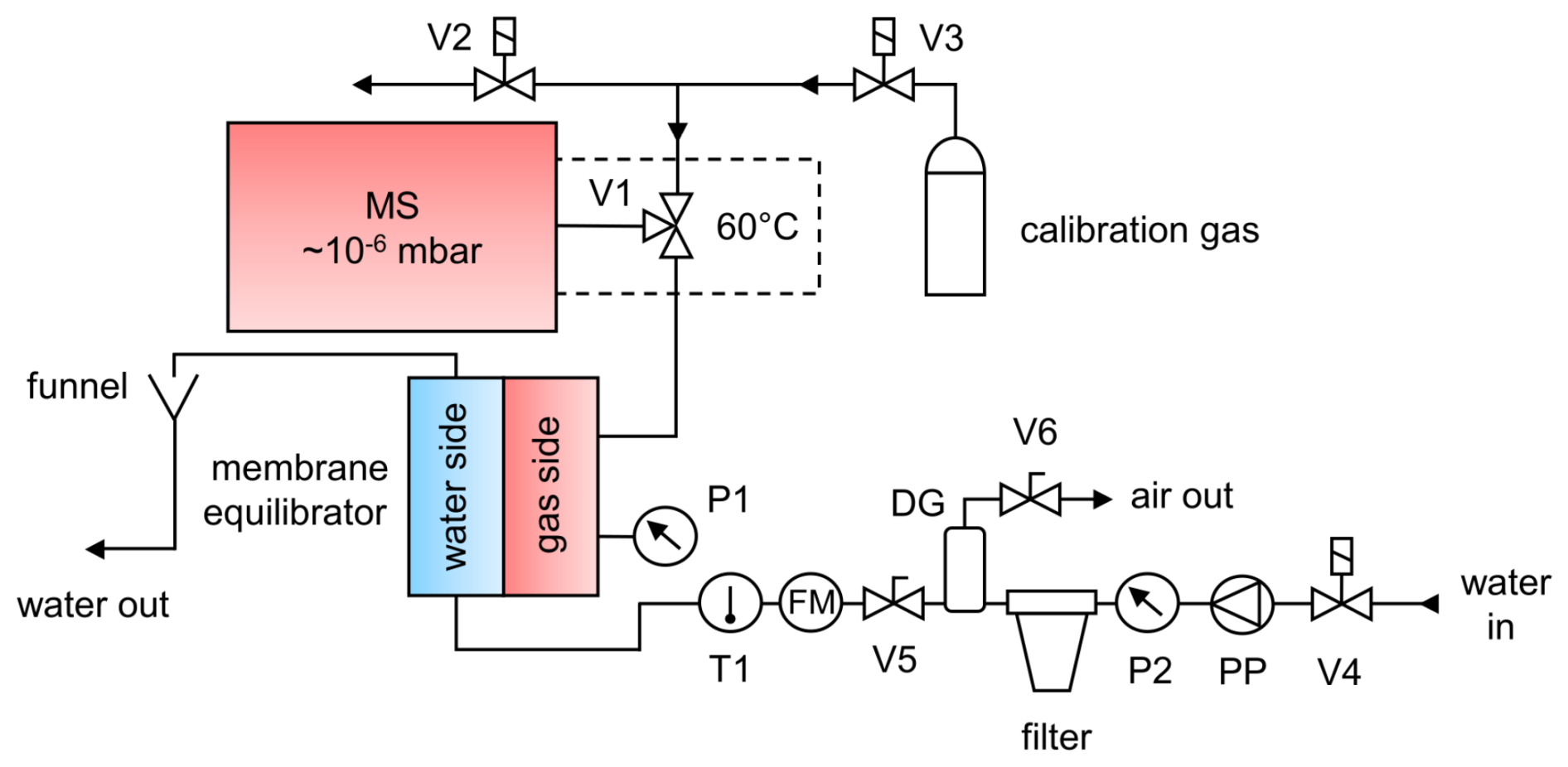
Figure 1 Schematic diagram of the Gas Equilibrium – Membrane-Inlet Mass Spectrometer (GE-MIMS) system. V1: two-position valve (computer-controlled). V2, V3 and V4: solenoid valves (computer-controlled). V5 and V6: valves. T1: temperature probe. P1 and P2: pressure sensors. PP: peristaltic pump. FM: flow meter. DG: degassing cylinder.

The membrane equilibrator used in this study was the Liqui-Cel mini-module cartridge (1.8×8.75, model G541), containing porous hollow fibers made of gas-permeable hydrophobic polypropylene. The fibers are compactly arranged in a polycarbonate housing and provide a total membrane surface area of 0.9 m² exposed to a water volume of 70 mL. Due to the relatively large gas room (140 mL), the continuous flow of gas into the MS (6 µL min⁻¹) caused a pressure drop on the gas side of only 0.2 ‰ and thus had almost no effect on the establishment of the equilibration process (see Appendix A).

In addition to the Liqui-Cel membrane, we tested a membrane equilibrator produced by PermSelect (PDMSXA-1.0), in which the gas exchange between the water and gas phases is mediated by dense, non-porous hollow fibers consisting of polydimethylsiloxane (PDMS). Since the gas exchange does not take place across pores, clogging by particles that may hamper the gas flux is avoided by these membranes. However, testing with the PermSelect membrane revealed that it is unsuitable for our application. For reasons that remain unclear, water accumulates on the gas side of the membrane, which could potentially be sucked into the inlet of the MS and block gas flow into it. Furthermore, it affects vacuum stability and interferes with accurate mass spectrometric measurements.

Water temperature in the GE-MIMS system is measured by a temperature probe (T1, PT100; accuracy 0.01 °C) located at the inlet of the membrane. The total gas tension is recorded by connecting a pressure sensor (P1) (SEN 3276, Kobold; precision 2 mbar) to the gas side of the membrane cartridge. A capillary connects the gas side of the equilibrator to the MS via V1.

A crucial aspect of the water flow system is ensuring that the water outlet is not positioned below the water level in the membrane equilibrator. Tests have shown that otherwise a suction effect occurs on the water side, which reduces the total gas pressure in the equilibrator and thus disturbs the gas-phase equilibrium.

Another aspect to be considered when using GE-MIMS for field studies is the effect of biofouling on membrane properties. Here, we suggest regularly cleaning or even replacing the membrane to maintain its performance. For field studies where there is a significant temperature difference between the water body under investigation and the laboratory, we recommend insulating the equilibrator to prevent the formation of water vapor condensate on the gas side of the membrane.

2.2 Mass spectrometry for N₂, Ar and O₂

A commercially available quadrupole mass spectrometer (QMS, GAM2000, InProcess Instruments) was used to analyze the gas composition on the gas side of the membrane equilibrator. A high vacuum (10⁻⁶ mbar) is generated within the MS through the combined use of a membrane pump and a turbomolecular pump. The sample gas is introduced into the ion source through a deactivated fused silica capillary (length 3 m and internal diameter 50 µm) connected to a two-position valve (V1; see Fig. 1). To enhance MS signal stability, these parts are housed within a heated enclosure maintained at a constant temperature of 60 °C.

Using V1, either the gas side of the equilibrator or the calibration gas is connected to the MS by a capillary. It is crucial that the two capillaries have identical properties (length 1.5 m and internal diameter 50 µm) in order to maintain a constant internal pressure within the MS. The capillaries' dimensions limit the gas flow rate to approximately 6 µL min⁻¹ according to the modified Hagen–Poiseuille equation (Cassar et al., 2009). This rate corresponds to a measured transfer time of approximately 80 s from the capillary inlet to detection.

During calibration, V3 connects the MS to the calibration gas, while V2 is opened to ambient air in order to prevent overpressure at V1. After calibration, V2 is closed in order to avoid contamination of the calibration line by ambient air through diffusion and to minimize its consumption.

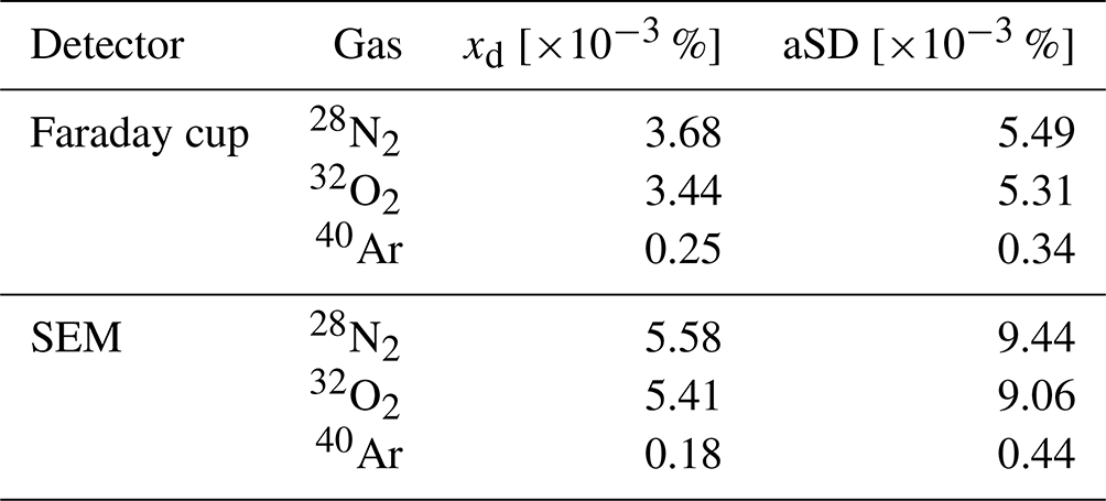
Within the ion source of the MS, the sample molecules and atoms are ionized by electron impact ionization (70 eV). They are then separated in the quadrupole analyzer based on their mass-to-charge ratio ($m/z$) and ultimately detected and quantified using a Faraday cup. Alternatively, a secondary electron multiplier (SEM) can be used for both detection and quantification. However, systematic measurements (see below) have shown that for N₂ and O₂ the standard deviation is twice as large and the accuracy decreases when using the SEM (Table 1), which may be due to its greater temperature sensitivity (Hoffmann et al., 2005; Khan et al., 2018).

Table 1 Performance parameters of the GAM 2000-MS obtained by repeated measurements of the gases in ambient air. x_d: mole fraction deviation between the measured and target values. aSD: absolute standard deviation. SEM: secondary electron multiplier.

For the quantification of N₂, O₂ and Ar, the respective ion currents can be extracted from the peaks of the nominal $m/z$ ratios in the mass spectra (N₂: $m/z=\mathrm{28}$, O₂: $m/z=\mathrm{32}$ and Ar: $m/z=\mathrm{40}$). During a 1 s measurement cycle, an ion current is detected for each gas species, which requires a measurement time of 340 ms per $m/z$ ratio. Interferences with CO₂ fragments (CO⁺, $m/z$ = 28) can be ignored, as discussed in Appendix B. For our laboratory tests, baseline correction was performed weekly using values at $m/z$ = 3. However, baseline stability may vary depending on the location or platform where the GE-MIMS is used. We recommend conducting additional tests during field operations in order to use field-specific conditions.

We used a standard gas to calibrate the MS regularly (gas compositions x(N₂): 78.1 %, x(O₂): 20.9 % and x(Ar): 1.0 %), which we had previously recalibrated with clean, dry air. Calibration using such a standard gas is particularly important in areas where the standard composition of air is affected by exhaust gases, e.g., on a VOS. In environments where air pollution can be ruled out, the ambient air can also be used as the standard (e.g., Cassar et al., 2009; Mächler et al., 2012; Manning et al., 2016). We used Ar as an internal standard in order to reduce the effect of temperature or pressure fluctuations within the MS. The calibration factors are given by the ratio $I_{\mathrm{X}}/I_{\mathrm{Ar}}$ (ratio of the currents for gases X and Ar) divided by the ratio $n_X/n_{\mathrm{Ar}}$ (ratio of the molar amounts of X and Ar in the standard gas). From this calibration procedure it follows that the elemental ratios X $/$ Ar for the analyzed gases (N₂ $/$ Ar, O₂ $/$ Ar and N₂ $/$ O₂) are the primary outcomes of our MS measurements. The elemental ratios then yield mole fractions for N₂, O₂ and Ar with respect to the sum of N₂, O₂ and Ar. These mole fractions are called “incomplete” mole fractions or, if only water vapor effects the composition of the air, “dry” mole fractions (the calculations are presented in Appendix B).

Regarding the performance of the MS, it is important to take into account the fact that the ionization process within the mass spectrometer is inherently pressure-dependent, resulting in variations in the ionization ratios of gases under different pressure conditions. To mitigate this, we effectively reduced the electron and ion densities in the ion formation region by adjusting the emission current. This resulted in enhanced linearity in ion yield and fragmentation at different pressures. Indeed, our observations indicate that, at pressures of 200 mbar above the calibration conditions (atmospheric pressure), the relative change in the molar fraction of N₂ was 0.4 %. However, a total equilibrium pressure (total gas tension) of gases dissolved in surface seawater of more than 200 mbar above the atmospheric pressure, e.g., by biological or temperature effects, can be excluded. The performance of the GAM 2000-MS was evaluated by conducting 60 replicate measurements of ambient air over a period of 6 h, with ambient air calibration of the system being carried out between measurements throughout the entire period. The average of the 60 measurements was used to calculate the performance parameters of the MS (Table 1).

3 Performance of the concentration measurements

3.1 Accuracy and precision

The partial pressures of N₂, O₂ and Ar in the gas room of the membrane equilibrator (p_i) can be calculated by a modification of Dalton's law (Eq. 1). Since incomplete mole fractions, which refer only to the total moles of the three considered gases ($x_i^{\prime }$; see Appendix A), are used, the total pressure in the headspace (p_t) must be corrected for gases that were not measured, such as water vapor. However, the MS-based determination of water vapor is challenging due to the lack of a suitable calibration medium and the potential for overlapping $m/z$ ratios, leading to imprecise measurements. Thus, water vapor is instead determined by assuming saturation at the given temperature and salinity (Ambrose and Lawrenson, 1972). The contribution of other gases, e.g., CO₂, to the total pressure is assumed to be very minor and is neglected. The partial pressure of the considered gases is therefore calculated as shown in Eq. (1):

$$\begin{array}{}\text{(1)}& p_i=x_i^{\prime }\cdot \left(p_{\mathrm{t}}-p{\mathrm{H}}_{\mathrm{2}}\mathrm{O}\right).\end{array}$$

Finally, the concentration of dissolved gases (c_i) in the water phase of the membrane equilibrator is calculated using the solubility constants obtained from Hamme and Emerson (2004) for N₂ and Ar and from Weiss (1970) for O₂, as shown in Eq. (2):

$$\begin{array}{}\text{(2)}& c_i=s_i\cdot p_i,\end{array}$$

with s the solubility constant [mol m⁻³ atm⁻¹] and p the partial pressure [atm⁻¹].

High instrument precision and accuracy are critical for measuring biogenic changes in N₂ and O₂ concentrations. This is particularly important in determinations of N₂ fixation in the Baltic Sea, as concentration deficits of only about 5 µmol N₂ L⁻¹ (derived from the depth-integrated N₂ fixation in Schneider et al., 2014a) with a background concentration of about 500 µmol N₂ L⁻¹ (at 20 °C) can be expected during moderate N₂ fixation activity in the central Baltic Sea.

The accuracy and precision of the concentration measurements were assessed by coupling the GE-MIMS system to a temperature-controlled bath (Huber CC-K15) filled with distilled water. The thermostat was set to a constant temperature (T = 18.5 ± 0.02 °C) and was open to the atmosphere in order to generate an equilibrium with atmospheric gases. The water was continuously recirculated through the membrane equilibrator at a flow rate of 2 L min⁻¹. Following calibration of the GE-MIMS system, the mole fractions x^′ of N₂, O₂ and Ar and the total pressure of the gas phase were continuously measured for 1 h. After an initial adjustment period, the measured values were averaged (Δt ∼ 20–60 min, Fig. 2) and used to determine the concentration (c_meas) and the absolute and relative standard deviations (aSD and rSD) of the concentrations of N₂, O₂ and Ar (Table 2).

Table 2 Results of a laboratory experiment in order to assess the accuracy and precision (2-fold aSD) of the GE-MIMS. rSD: relative standard deviation.

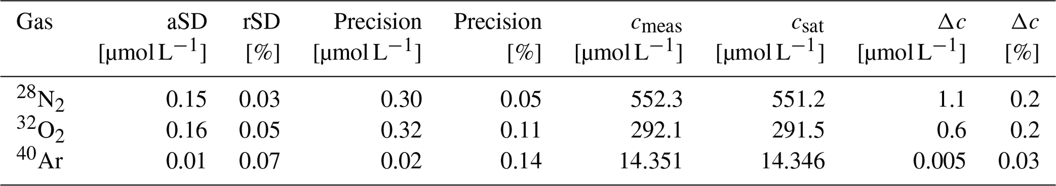
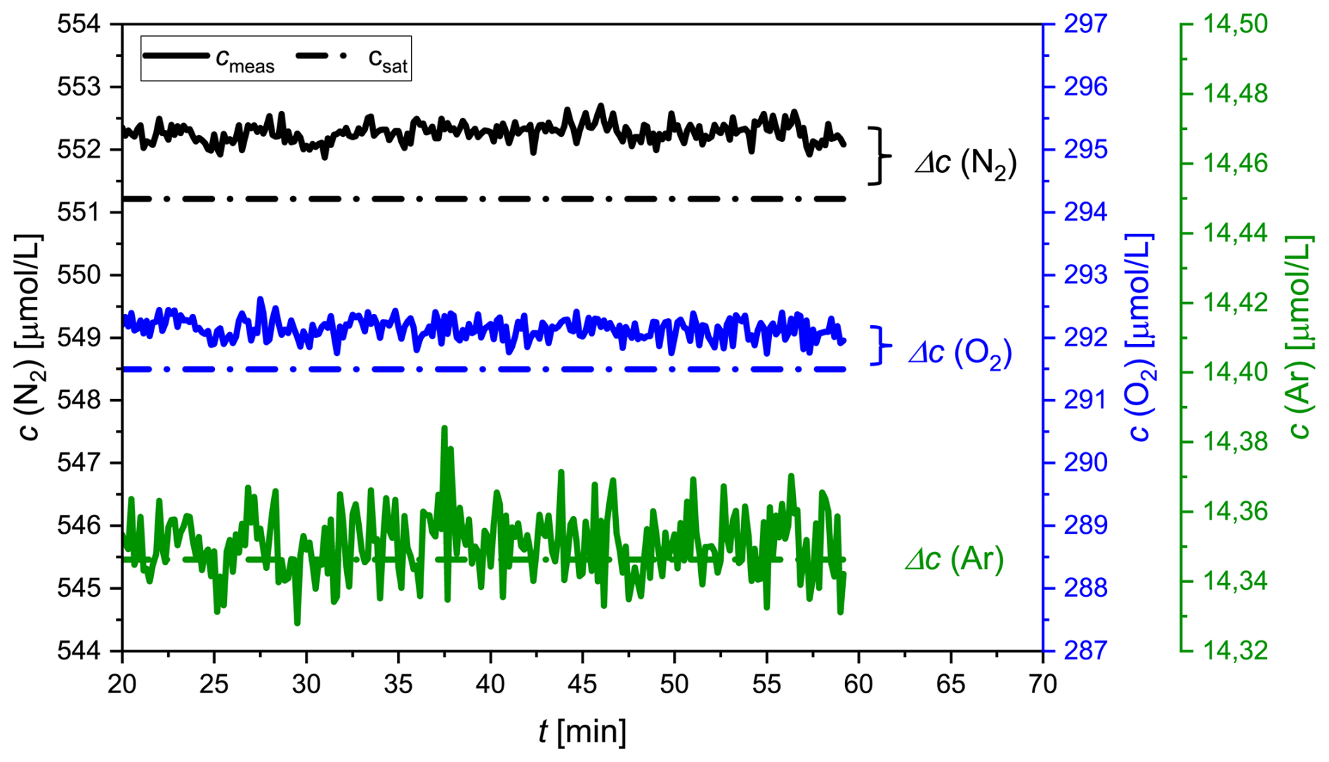
Figure 2 Concentration measurements of N₂ (black), O₂ (blue) and Ar (green) in distilled water equilibrated with ambient air during a laboratory experiment. While the measured values (c_meas) are indicated by the solid lines, the saturation values (c_sat) are indicated by the dotted lines.

The measured concentrations are presented together with the expected saturation concentrations (Hamme and Emerson, 2004; Weiss, 1970) in Fig. 2 and Table 2. The absolute standard deviation was very similar for N₂ and O₂, ranging from 0.15 to 0.16 µmol L⁻¹. The measured concentration of Ar had an aSD that was 1 order of magnitude smaller. Additionally, the data indicated a 0.2 % offset for both N₂ and O₂ measurements. For Ar, the averaged offset was 0.03 %, an order of magnitude smaller than for the other gases (Table 2). The accuracy is given by the concentration difference (Δc) between the measured value (c_meas) and the saturation value (c_sat) of N₂, O₂ and Ar, as presented in Table 2. The precision is reported as the 2-fold aSD.

The deviation of the measured N₂ concentration (Δc (N₂) = 1.1 µmol L⁻¹, Table 2) from the theoretical saturation values indicates that a moderately strong N₂ fixation episode of 5 µmol-N₂ L⁻¹ (derived from Schneider et al., 2014a) can be determined with an accuracy of about 20 %. This uncertainty also refers to the NCP associated with the N₂ fixation, which under average conditions contributes 20 %–26 % to the total annual NCP (Schneider and Müller, 2018).

3.2 Equilibration kinetics

3.2.1 Theory

The fundamental principle of a membrane equilibrator is that an equilibration process takes place between the partial pressures (p) of the water side (subscript “w”) and the gas side (subscript “g”) when they are separated by a gas-permeable membrane. To derive a mathematical expression for the dependence of the equilibration time (τ) on the water flow rate (Q_w), we first consider the continuous flow to be a step-wise renewal of the water, where each time step corresponds to the mean residence time of the water in the equilibrator (water volume divided by water flow). It is then assumed that an equilibrium between the “stagnant” water and the gas phase is established during each time step. This is a plausible assumption in view of the dimensions of the membrane equilibrator (3M data sheet, 2021). The average thicknesses of the gas and water layers in the equilibrator are only 140 and 70 µm, respectively, and allow almost spontaneous equilibration. However, interpretations of the equilibrium must take into account the fact that gas exchange during the equilibration process affects both the gas phase and the dissolved phase. The partial pressure distribution after the first time step is given by Eq. (3), according to which, at equilibrium, the initial p_g,0 altered by Δp_g must be equal to the initial p_w,0 altered by Δp_w (Δp_w,g refers to absolute changes):

$$\begin{array}{}\text{(3)}& p_{\mathrm{g},\mathrm{0}}-\mathrm{\Delta }{p}_{\mathrm{g}}=p_{\mathrm{w},\mathrm{0}}+\mathrm{\Delta }{p}_{\mathrm{w}}.\end{array}$$

The initial Δp₀ can thus be expressed as shown in Eq. (4):

$$\begin{array}{}\text{(4)}& \mathrm{\Delta }{p}_{\mathrm{0}}=\mathrm{\Delta }{p}_{\mathrm{g}}+\mathrm{\Delta }{p}_{\mathrm{w}}.\end{array}$$

Δp_g and Δp_w can be expressed by the flux of moles (Δn) across the membrane, as shown in Eqs. (5) and (6):

$$\begin{array}{}\text{(5)}& \mathrm{\Delta }{p}_{\mathrm{g}}={\displaystyle \frac{\mathrm{\Delta }n\cdot R\cdot T}{V_{\mathrm{g}}}},\end{array}$$

$$\begin{array}{}\text{(6)}& \mathrm{\Delta }{p}_{\mathrm{w}}={\displaystyle \frac{\mathrm{\Delta }n}{V_{\mathrm{w}}\cdot s}}\cdot ,\end{array}$$

with R the universal gas constant [m³ atm mol⁻¹ K⁻¹], T the absolute temperature [K] and V the volume [m³].

Combining Eqs. (5) and (6) describes Δp_w as a function of Δp_g and yields Eq. (7):

$$\begin{array}{}\text{(7)}& \mathrm{\Delta }{p}_{\mathrm{w}}={\displaystyle \frac{\mathrm{\Delta }{p}_{\mathrm{g}}\cdot V_{\mathrm{g}}}{V_{\mathrm{w}}\cdot s\cdot R\cdot T}},\end{array}$$

which together with Eq. (4) yields Eq. (8):

$$\begin{array}{}\text{(8)}& \mathrm{\Delta }{p}_{\mathrm{0}}=\mathrm{\Delta }{p}_{\mathrm{g}}+{\displaystyle \frac{\mathrm{\Delta }{p}_{\mathrm{g}}\cdot V_{\mathrm{g}}}{V_{\mathrm{w}}\cdot s\cdot R\cdot T}}.\end{array}$$

The ratio of Δp_g to the original Δp₀ is described by Eq. (9):

$$\begin{array}{}\text{(9)}& {\displaystyle \frac{\mathrm{\Delta }{p}_{\mathrm{g}}}{\mathrm{\Delta }{p}_{\mathrm{0}}}}={\displaystyle \frac{\mathrm{1}}{\mathrm{1}+\frac{V_{\mathrm{g}}}{V_{\mathrm{w}}\cdot s\cdot R\cdot T}}},\end{array}$$

which shows that, after equilibration, the change in Δp_g in relation to the initial Δp₀ depends on the ratio of the gas and water volumes and the solubility of the considered gas. For our Liqui-Cel membrane, the volume ratio $V_{\mathrm{w}}/V_{\mathrm{g}}$ is 0.5 (3M data sheet, 2021) and results in a 0.8 % change in Δp_g for N₂ with respect to the initial Δp₀, whereas, conversely, Δp_w changes by 99.2 % of the initial Δp₀. This means that, at equilibrium, the partial pressure of the dissolved phase is close to that of the initial gas phase. However, our approach is based on a gas-phase partial pressure that is at equilibrium with water widely unaffected by gas exchange: $\mathrm{\Delta }{p}_{\mathrm{g}}/\mathrm{\Delta }{p}_{\mathrm{0}}\approx \mathrm{1}$ or $\mathrm{\Delta }{p}_{\mathrm{w}}/\mathrm{\Delta }{p}_{\mathrm{0}}\approx \mathrm{0}$. Even a 100-fold increase in the ratio to $V_{\mathrm{w}}/V_{\mathrm{g}}=\mathrm{50}$ would only yield a value of 0.45 for $\mathrm{\Delta }{p}_{\mathrm{g}}/\mathrm{\Delta }{p}_{\mathrm{0}}$. These calculations indicate that the water volume must approach infinity to achieve a 100 % adjustment of p_g,0 to the initial p_w,0. The latter condition can be approximated by repeated renewal of the water through continuous pumping.

Equation (9) was derived for the first time step, but it is of course valid for any time step (i) and the corresponding partial pressure difference Δp. Furthermore, the change in p_g may be interpreted as a reduction in the partial pressure difference after each water renewal. This may be approximated by the differential Eq. (10) using i as a variable:

$$\begin{array}{}\text{(10)}& {\displaystyle \frac{\mathrm{d}\left(\mathrm{\Delta }p\right)}{\mathrm{d}i}}={\displaystyle \frac{-\mathrm{1}}{\mathrm{1}+\frac{V_{\mathrm{g}}}{V_{\mathrm{w}}\cdot s\cdot R\cdot T}}}\cdot (\mathrm{\Delta }p{)}_i.\end{array}$$

This leads to Eq. (11):

$$\begin{array}{}\text{(11)}& \mathrm{d}\left(\ln \mathrm{\Delta }p\right)={\displaystyle \frac{-\mathrm{d}i}{\mathrm{1}+\frac{V_{\mathrm{g}}}{V_{\mathrm{w}}\cdot s\cdot R\cdot T}}}.\end{array}$$

Integrating Eq. (11) yields Eq. (12):

$$\begin{array}{}\text{(12)}& \mathrm{\Delta }p=\mathrm{\Delta }{p}_{\mathrm{0}}\cdot \exp \left({\displaystyle \frac{-i}{\mathrm{1}+\frac{V_{\mathrm{g}}}{V_{\mathrm{w}}\cdot s\cdot R\cdot T}}}\right).\end{array}$$

Since i is given by the elapsed time, t, divided by the residence time, t_r, Eq. (12) can be expressed by Eq. (13):

$$\begin{array}{}\text{(13)}& \mathrm{\Delta }p=\mathrm{\Delta }{p}_{\mathrm{0}}\cdot \exp \left[{\displaystyle \frac{-t}{t_{\mathrm{r}}\cdot \left(\mathrm{1}+\frac{V_{\mathrm{g}}}{V_{\mathrm{w}}\cdot s\cdot R\cdot T}\right)}}\right],\end{array}$$

which describes the exponential development of the partial pressure difference towards equilibrium (Δp=0).

Introducing the residence time under water flow conditions, τ, gives

$$\begin{array}{}\text{(14)}& \mathrm{\Delta }p=\mathrm{\Delta }{p}_{\mathrm{0}}\cdot \exp \left[{\displaystyle \frac{-t}{\mathit{\tau }}}\right],\end{array}$$

where τ is given as shown in Eq. (15):

$$\begin{array}{}\text{(15)}& \mathit{\tau }=t_{\mathrm{r}}\cdot \left(\mathrm{1}+{\displaystyle \frac{V_{\mathrm{g}}}{V_{\mathrm{w}}\cdot s\cdot R\cdot T}}\right).\end{array}$$

Equation (14) indicates that, after a time t=τ, only $\mathrm{1}/e$ of the original difference in the partial pressure remains. This implies that the equilibrium state has already reached approximately 63 %. Consequently, after 4 times the equilibration time has elapsed, equilibrium has reached 99 %.

Since the residence time is given by the water volume divided by the water flow rate Q_w,

$$\begin{array}{}\text{(16)}& t_{\mathrm{r}}={\displaystyle \frac{V_{\mathrm{w}}}{Q_{\mathrm{w}}}}.\end{array}$$

Eq. (17) is obtained:

$$\begin{array}{}\text{(17)}& \mathit{\tau }={\displaystyle \frac{V_{\mathrm{w}}\cdot \left(\mathrm{1}+\frac{V_{\mathrm{g}}}{V_{\mathrm{w}}\cdot s\cdot R\cdot T}\right)}{Q_{\mathrm{w}}}}.\end{array}$$

An example is provided as follows: for the Liqui-Cel contactor used in our study and at a flow rate of 2 L min⁻¹, τ is 4.3 min for N₂, 2.2 min for O₂ and 2.0 min for Ar. The dependence of the equilibration time on water flow as well as on the solubility of the considered gas and the gas volume can be seen in Fig. 3a, b, which depicts the hyperbolically shaped functions described by Eq. (17); a significant increase in τ occurs at a water flow rate of < 500 mL min⁻¹. The maximum flow of the membrane used in our study, according to the manufacturer's specification, is 3000 mL min⁻¹. Figure 3a shows that, due to the solubilities of O₂ and Ar, their τ values are very similar, while the τ value of N₂ is about twice as high. A reduction in the gas volume of the membrane equilibrator leads to a corresponding decrease in τ (Fig. 3b).

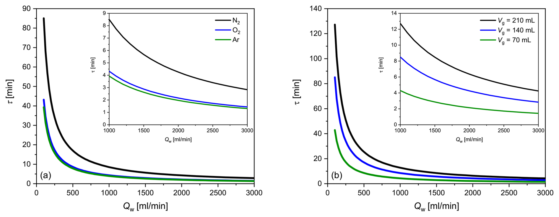
Figure 3 Theoretically determined dependence of the equilibration time τ on the water flow rate Q_w using the Liqui-Cel 1.8×8.75 contactor for (a) different gas solubilities (N₂, O₂ and Ar) and (b) N₂ and different gas side volumes of the membrane equilibrator (V_g of the Liqui-Cel contactor: 140 mL). The insets show the typical flow rate ranges at higher resolution.

The values for the different variables used in the previous calculations and figures are as follows:

•  

  $R\cdot T=\mathrm{2.39}\times {\mathrm{10}}^{-\mathrm{2}}$ m³ atm mol⁻¹ (T=18 °C);

•  

  $V_{\mathrm{w}}=\mathrm{0.7}\times {\mathrm{10}}^{-\mathrm{4}}$ m³ (3M data sheet, 2021);

•  

  $V_{\mathrm{g}}=\mathrm{1.4}\times {\mathrm{10}}^{-\mathrm{4}}$ m³ (3M data sheet, 2021);

•  

  s(N₂)=0.695 mol m⁻³ atm⁻¹ (Hamme and Emerson, 2004: T=18 °C, salinity = 7 PSU);

•  

  s(Ar) = 1.519 mol m⁻³ atm⁻¹ (Hamme and Emerson, 2004: T=18 °C, salinity = 7 PSU); and

•  

  s(O₂) =1.379 mol m⁻³ atm⁻¹ (Weiss, 1970: T=18 °C, salinity = 7 PSU).

3.2.2 Measurement of τ

The equilibration time (τ) of the membrane equilibrator used in this study (Liqui-Cel 1.7×8.75) was also determined experimentally under flow-through conditions. For this purpose, 100 L containers were filled with tap water and allowed to rest for at least 1 d to allow for the development of a homogeneous water mass in approximate equilibrium with the atmosphere. A transmembrane partial pressure difference was generated by initially flushing the gas side of the membrane equilibrator with N₂. Subsequently, the water (T≈18 °C) from the container was pumped through the water side at a flow rate of 2 L min⁻¹ using the peristaltic pump. Adjustments of the N₂, O₂ and Ar partial pressures in the gas room to match those of these gases dissolved in water were recorded by MS determination of the mole fractions and measurement of the total pressure, as described in Sect. 3.1. Figure 4a shows an increase in the N₂ partial pressure after the gas side was flushed with N₂, followed by a decline due to equilibration with the partial pressure of N₂ dissolved in the water. The resulting plateau after approximately 30 min was considered to indicate equilibrium with atmospheric gases. The temporal evolution of the partial pressure difference on the gas side between the value at time t, p_g (t), and the equilibrium value indicated by the plateaued partial pressure at 30 min, p_g (eq), can be described by the exponential function shown in Eq. (18), which corresponds to Eq. (14):

$$\begin{array}{}\text{(18)}& p_{\mathrm{g}}\left(t\right)-p_{\mathrm{g}}\left(\mathrm{eq}\right)=\left[p_{\mathrm{g}}\left(t_{\mathrm{0}}\right)-p_{\mathrm{g}}\left(\mathrm{eq}\right)\right]\cdot e^{\left(\frac{-t}{\mathit{\tau }}\right)}.\end{array}$$

Linearization of Eq. (18) yields an equation where ln[p_g (t) − p_g (eq)] is a linear function of t with a slope that corresponds to the reciprocal equilibration time; see Eq. (19):

$$\begin{array}{}\text{(19)}& \ln \left[p_{\mathrm{g}}\left(t\right)-p_{\mathrm{g}}\left(\mathrm{eq}\right)\right]=-{\displaystyle \frac{\mathrm{1}}{\mathit{\tau }}}\cdot t+\ln \left[p_{\mathrm{g}}\left(t_{\mathrm{0}}\right)-p_{\mathrm{g}}\left(\mathrm{eq}\right)\right].\end{array}$$

The equilibration time τ was then determined from a regression line for ln[p_g (t)−p_g (eq)] as a function of t (Fig. 4b). The experiment described above was conducted three times, resulting in average e-fold equilibration times ± aSD of τ (N₂) = 4.8±0.1 min, τ (O₂) = 3.2±0.1 min and τ(Ar) = 3.0±0.2 min. These values differ from those determined theoretically using Eq. (17) but show the same order of magnitude. The deviations are attributed to the simplified assumptions inherent in the model. Critical points are that the model does not consider continuous water flow but the transport of discrete water parcels through the equilibrator and that the assumption of perfect equilibrium was generated repeatedly after each renewal (residence time) of the water in the membrane equilibrator.

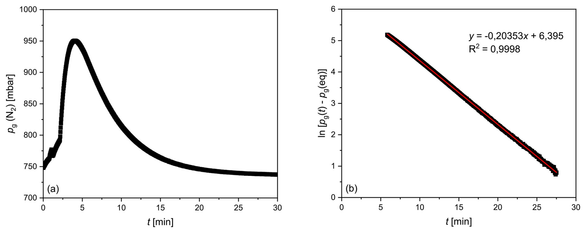
Figure 4 Results of an experiment to determine the equilibration time for N₂. (a) p_g (N₂) as a function of time. (b) The logarithmic presentation of the difference between the partial pressure of N₂ at any time t and after equilibrium is reached, as a function of time. The reciprocal slope of the regression line represents the e-fold equilibration time (τ).

The different equilibration times for the considered gases can be attributed to their different solubility constants, according to Eq. (17), with those of O₂ and Ar being similar and significantly below that of N₂. Compared with the τ (N₂ $/$ Ar) = 12 min achieved by coupling a MS to a spray-type equilibrator (Schmale et al., 2019), GE-MIMS is nearly 3 times faster. Compared with other membrane equilibrator setups, where τ (Ar) = 4 min (Manning et al., 2016) or τ (O₂ $/$ Ar) = 7.75 min (Cassar et al., 2009), our system provides slightly better temporal resolution.

If the GE-MIMS system is installed on a VOS, the spatial resolution (footprint) is given by the equilibration time and the ship's speed. Assuming an almost perfect equilibration after 4 τ and a typical ferry speed of about 20 kn results in a spatial resolution of approximately 12 km for N₂, which is considered the minimum scale for regional averaging of field data.

4 Quantification of biogeochemical process rates

The determination of biogeochemical process rates requires measurements of the respective variables as a function of time. The use of a VOS traveling across successive transects as a platform for GE-MIMS would enable the generation of a concentration time series over large areas such as the Baltic Proper (Schneider et al., 2007; Gülzow et al., 2011).

Any change in the N₂ concentration can be described as the effect of N₂ fixation and N₂ gas exchange with the atmosphere (Eq. 20) if vertical mixing across the thermocline is ignored. The latter is justified since N₂ fixation typically takes place at low wind speeds (<5 m s⁻¹) that lead to a rising thermocline and warming of the surface layer (up to 22 °C) (Müller et al., 2021):

$$\begin{array}{}\text{(20)}& \mathrm{\Delta }{\mathrm{N}}_{\mathrm{2}}=\mathrm{\Delta }{\mathrm{N}}_{\mathrm{2},\mathrm{fix}}+\mathrm{\Delta }{\mathrm{N}}_{\mathrm{2},\mathrm{gas}}.\end{array}$$

The concentration change due to gas exchange (ΔN_2,gas) during Δt (e.g., the time between two transects) within the mixed-layer depth, z_mix, is expressed by Eq. (21):

$$\begin{array}{}\text{(21)}& \mathrm{\Delta }{\mathrm{N}}_{\mathrm{2},\mathrm{gas}}=k_{\mathrm{660}}\cdot {\left({\displaystyle \frac{{\mathit{Sc}}_{{\mathrm{N}}_{\mathrm{2}}}}{\mathrm{660}}}\right)}^{-\mathrm{0.5}}\cdot \left({\stackrel{\mathrm{‾}}{\mathrm{N}}}_{\mathrm{2},\mathrm{sat}}-{\stackrel{\mathrm{‾}}{\mathrm{N}}}_{\mathrm{2}}\right)\cdot {\displaystyle \frac{\mathrm{\Delta }t}{z_{\mathrm{mix}}}},\end{array}$$

where Sc is the Schmidt number (Wanninkhof, 1992) and ${\stackrel{\mathrm{‾}}{\mathrm{N}}}_{\mathrm{2},\mathrm{sat}}$ and ${\stackrel{\mathrm{‾}}{\mathrm{N}}}_{\mathrm{2}}$ represent the values of the saturation concentration, averaged over a period of time (e.g., between two consecutive transects) and calculated based on the respective averaged temperature and salinity, and the measured concentration. The transfer velocity of gas exchange (k₆₆₀) varies with wind speed and can be estimated using parameterizations such as that suggested by Wanninkhof et al. (2009). However, especially at low wind speeds and during periods of increased OM production, this method is subject to considerable uncertainties. For example, the presence of organic surface films can significantly reduce gas exchange, a phenomenon that current transfer velocity parameterizations do not adequately address. Therefore, concurrent Ar measurements are included to circumvent the uncertainties in using parameterizations of the transfer velocity. This approach is based on the observation that N₂ fixation events usually coincide with a significant increase in surface temperature (Schneider et al., 2014b; Schmale et al., 2019), such that the partial pressure of Ar in the surface water increases, which in turn leads to an Ar flux into the atmosphere. The change in the Ar concentration due to gas exchange at the water surface can be calculated using Eq. (22), which is similar to Eq. (21):

$$\begin{array}{}\text{(22)}& \mathrm{\Delta }{\mathrm{Ar}}_{\mathrm{gas}}=k_{\mathrm{660}}\cdot {\left({\displaystyle \frac{{\mathit{Sc}}_{\mathrm{Ar}}}{\mathrm{660}}}\right)}^{-\mathrm{0.5}}\cdot \left({\mathrm{Ar}}_{\mathrm{sat}}-\mathrm{Ar}\right)\cdot {\displaystyle \frac{\mathrm{\Delta }t}{z_{\mathrm{mix}}}}.\end{array}$$

Nitrogen gas exchange can then be quantified without explicitly calculating k₆₆₀, since combining Eqs. (21) and (22) yields Eq. (23):

$$\begin{array}{}\text{(23)}& \mathrm{\Delta }{\mathrm{N}}_{\mathrm{2},\mathrm{gas}}=\mathrm{\Delta }\mathrm{Ar}\cdot {\left({\displaystyle \frac{{\mathit{Sc}}_{\mathrm{N}\mathrm{2}}}{{\mathit{Sc}}_{\mathrm{Ar}}}}\right)}^{-\mathrm{0.5}}\cdot {\displaystyle \frac{{\stackrel{\mathrm{‾}}{\mathrm{N}}}_{\mathrm{2},\mathrm{sat}}-{\stackrel{\mathrm{‾}}{\mathrm{N}}}_{\mathrm{2}}}{{\stackrel{\mathrm{‾}}{\mathrm{Ar}}}_{\mathrm{sat}}-\stackrel{\mathrm{‾}}{\mathrm{Ar}}}}.\end{array}$$

Finally, the difference in the nitrogen concentration due to N₂ fixation for a certain time interval can be obtained using Eq. (24):

$$\begin{array}{}\text{(24)}& \mathrm{\Delta }{\mathrm{N}}_{\mathrm{2},\mathrm{fix}}=\mathrm{\Delta }{\mathrm{N}}_{\mathrm{2}}-\mathrm{\Delta }\mathrm{Ar}\cdot {\left({\displaystyle \frac{{\mathit{Sc}}_{{\mathrm{N}}_{\mathrm{2}}}}{{\mathit{Sc}}_{\mathrm{Ar}}}}\right)}^{-\mathrm{0.5}}\cdot {\displaystyle \frac{{\stackrel{\mathrm{‾}}{\mathrm{N}}}_{\mathrm{2},\mathrm{sat}}-{\stackrel{\mathrm{‾}}{\mathrm{N}}}_{\mathrm{2}}}{{\stackrel{\mathrm{‾}}{\mathrm{Ar}}}_{\mathrm{sat}}-\stackrel{\mathrm{‾}}{\mathrm{Ar}}}}.\end{array}$$

Because of the low wind speed and the surface accumulation of OM during a cyanobacterial bloom, it is assumed that gas exchange is of minor importance and that the temporal change in the measured nitrogen concentration ΔN₂ is the main term (Wasmund, 1997; Lips and Lips, 2008; Schmale et al., 2019).

Equation (24) includes implicitly the calculation of k₆₆₀, which can be determined explicitly from the Ar measurement by the use of Eq. (22):

$$\begin{array}{}\text{(25)}& k_{\mathrm{660}}={\displaystyle \frac{\mathrm{\Delta }\mathrm{Ar}\cdot z_{\mathrm{mix}}}{{\left({\mathit{Sc}}_{\mathrm{Ar}}/\mathrm{660}\right)}^{-\mathrm{0.5}}\cdot \left({\stackrel{\mathrm{‾}}{\mathrm{Ar}}}_{\mathrm{sat}}-\stackrel{\mathrm{‾}}{\mathrm{Ar}}\right)\cdot \mathrm{\Delta }t}}.\end{array}$$

Therefore, continuous measurements with our newly developed GE-MIMS system can also be used to determine k₆₆₀, provided the mixed-layer depth (z_mix) can be estimated, e.g., by modeling the surface water temperature and salinity profiles (Gräwe et al., 2019).

5 Conclusions

The results from our laboratory tests demonstrated that the GE-MIMS system is capable of directly determining cyanobacterial N₂ consumption and potentially also the associated O₂ production resulting from photosynthesis triggered by N₂ fixation. Ar concentrations for both the parameterization of air–sea gas exchange and the reconstruction of abiotic background concentrations of biogeochemically active gases such as N₂ and O₂ could be measured with high precision and accuracy. Our measurement system is based on the same principle as that of Schmale et al. (2019), but it uses a membrane equilibrator, which in contrast to bubble or shower-type equilibrators does not require ventilation and therefore constitutes a closed system. This ensures that the partial pressures in the gas phase are truly in equilibrium with the dissolved gases rather than merely in a steady state (Schneider et al., 2007).

The individual components are designed to allow autonomous long-term operation of the measurement system, particularly when installed on a VOS, such as that currently used for continuous pCO₂ measurements in the Baltic Sea (Gülzow et al., 2011; Schneider et al., 2014b; Jacobs et al., 2021). The resulting N₂, O₂ and Ar concentration time series will facilitate determinations of N₂ fixation rates and potentially NCP in selected regions of the Baltic Sea. The temporal dynamics of the abovementioned biogeochemical processes can also be investigated. Furthermore, synchronous measurements of surface N₂(Ar) and pCO₂ take advantage of both the direct determination of N₂ consumption by fixation and the high sensitivity of the CO₂ approach to production events (Schneider and Müller, 2018). The main limitations of existing approaches to quantifying N₂ fixation, which result from the analysis of discrete samples and the use of the elemental composition of POM, are thus circumvented. Furthermore, the possibility of averaging over larger spatial scales due to the operation of the GE-MIMS system on a VOS enhances its compatibility with process-based model results, which typically have a spatial resolution of several kilometers.

Appendix A: Pressure effect of the gas flow into the mass spectrometer

To estimate the effect of the continuous flow of gas into the MS (6 µL min⁻¹) on the pressure in the gas room (p_g), the development of a steady state in the gas room is considered. The latter is based on a balance between the gas flow into the MS (F_MS) and the flux of dissolved gases into the gas room (F_g), which are given by Eqs. (A1) and (A2):

$$\begin{array}{}\text{(A1)}& {\displaystyle }{F}_{\mathrm{MS}}=Q_{\mathrm{v}}\cdot {\displaystyle \frac{p_{\mathrm{g}}}{R\cdot T}},\left[\mathrm{mol}{\mathrm{s}}^{-\mathrm{1}}\right],\text{(A2)}& {\displaystyle }{F}_{\mathrm{g}}=k_n\cdot A\cdot \left(p_{\mathrm{atm}}-p_{\mathrm{g}}\right),\left[\mathrm{mol}{\mathrm{s}}^{-\mathrm{1}}\right],\end{array}$$

with Q_v the volume flow into the MS $\mathrm{1}\times {\mathrm{10}}^{-\mathrm{10}}$ m³ s⁻¹, k_n the transfer coefficient $\mathrm{2.21}\times {\mathrm{10}}^{-\mathrm{5}}$ mol s⁻¹ m⁻² atm⁻¹ (derived from the experimentally determined equilibration time; see Appendix C), A the membrane area 0.92 m², R⋅T = $\mathrm{2.39}\times {\mathrm{10}}^{-\mathrm{2}}$ m³ atm mol⁻¹ (T=18 °C), p_g the pressure in the gas room [atm] and p_atm the total pressure of the dissolved gases (approximately 1 atm).

Equations (A1) and (A2) lead to the mass balance described in Eq. (A3) for the steady state:

$$\begin{array}{}\text{(A3)}& Q_{\mathrm{v}}\cdot {\displaystyle \frac{p_{\mathrm{g}}}{R\cdot T}}=k_n\cdot A\cdot \left(p_{\mathrm{atm}}-p_{\mathrm{g}}\right).\end{array}$$

Rearranging Eq. (A3) yields an expression that describes the effect of the gas flow into the MS through the ratio between the pressure in the gas room (p_g) and the “true” equilibrium pressure (p_atm) that was assumed to be 1 atm, as shown in Eq. (A4):

$$\begin{array}{}\text{(A4)}& {\displaystyle \frac{p_{\mathrm{g}}}{p_{\mathrm{atm}}}}={\displaystyle \frac{\mathrm{1}}{\mathrm{1}+\frac{Q_{\mathrm{v}}}{R\cdot T\cdot k_{\mathrm{n}}\cdot A}}}.\end{array}$$

Using the values for the variables in Eq. (A4), as given above, results in a ratio $p_{\mathrm{g}}/p_{\mathrm{atm}}=\mathrm{0.9998}$, which means that the pressure in the gas room deviated by 0.2 ‰ from the equilibrium total pressure.

Appendix B: Evaluation of mass spectrometric data

In the initial step, ion currents corresponding to the specific mass-to-charge ratios of the following gases are measured using the mass spectrometer: N₂: $m/z=\mathrm{28}$, O₂: $m/z=\mathrm{32}$ and Ar: $m/z=\mathrm{40}$. We are aware that the $m/z$ ratio for nitrogen may include interferences with other fragment ions, such as from carbon dioxide (CO⁺). However, based on the paper of Burlacot et al. (2020), only 9.81 % of the primary CO₂ signal at $m/z$ = 44 is fragmented into the CO⁺ ion at $m/$z = 28. Assuming a CO₂ concentration close to atmospheric equilibrium concentrations, this would correspond to around 40 ppm of CO, which interferes with the N₂ quantification (at atmospheric N₂ concentrations of 78 %). This level of interference is negligible. Furthermore, regarding envisaged measurements on a VOS in the Baltic Sea, the risk of interference becomes even lower because CO₂ in the surface waters of the Baltic Sea is strongly undersaturated with respect to atmospheric CO₂ during periods of N₂ fixation due to concurrent biological production (Schneider et al., 2007).

For calibration, a gas mixture characterized by precisely defined molar ratios ($n/n$) of N₂, O₂ and Ar is used to transform the ion currents (I) into mole fractions (x). Therefore, calibration factors are determined which are based on the ion currents of N₂ and O₂ normalized to the ion current of Ar as an internal standard. The calibration factors are then obtained by relating the normalized ion currents to the corresponding molar ratios between the considered gas and Ar, as shown in Eqs. (B1) and (B2):

$$\begin{array}{}\text{(B1)}& {\displaystyle }{F}_{\mathrm{cal},{\mathrm{N}}_{\mathrm{2}}}={\displaystyle \frac{\frac{I_{{\mathrm{N}}_{\mathrm{2}}}}{I_{\mathrm{Ar}}}}{\frac{n_{{\mathrm{N}}_{\mathrm{2}}}}{n_{\mathrm{Ar}}}}},\text{(B2)}& {\displaystyle }{F}_{\mathrm{cal},{\mathrm{O}}_{\mathrm{2}}}={\displaystyle \frac{\frac{I_{{\mathrm{O}}_{\mathrm{2}}}}{I_{\mathrm{Ar}}}}{\frac{n_{{\mathrm{O}}_{\mathrm{2}}}}{n_{\mathrm{Ar}}}}}.\end{array}$$

Once the calibration factors are determined, measurements of the ion currents for N₂, O₂ and Ar yield the molar ratios $n_{{\mathrm{O}}_{\mathrm{2}}}/n_{\mathrm{Ar}}$, $n_{{\mathrm{N}}_{\mathrm{2}}}/n_{\mathrm{Ar}}$ and, consequently, $n_{{\mathrm{O}}_{\mathrm{2}}}/n_{{\mathrm{N}}_{\mathrm{2}}}$. These can be used to calculate the mole fractions (x^′) of N₂, O₂ and Ar with respect to the sum of N₂, O₂ and Ar, resulting in Eqs. (B3) to (B5):

$$\begin{array}{}\text{(B3)}& {\displaystyle \frac{n_{{\mathrm{O}}_{\mathrm{2}}}}{n_{\mathrm{Ar}}}}+{\displaystyle \frac{n_{{\mathrm{N}}_{\mathrm{2}}}}{n_{\mathrm{Ar}}}}+\mathrm{1}={\displaystyle \frac{\mathrm{1}}{x_{\mathrm{Ar}}^{\prime }}},\text{(B4)}& {\displaystyle \frac{n_{{\mathrm{O}}_{\mathrm{2}}}}{n_{{\mathrm{N}}_{\mathrm{2}}}}}+{\displaystyle \frac{n_{\mathrm{Ar}}}{n_{{\mathrm{N}}_{\mathrm{2}}}}}+\mathrm{1}={\displaystyle \frac{\mathrm{1}}{x_{{\mathrm{N}}_{\mathrm{2}}}^{\prime }}},\text{(B5)}& {\displaystyle \frac{n_{{\mathrm{N}}_{\mathrm{2}}}}{n_{{\mathrm{O}}_{\mathrm{2}}}}}+{\displaystyle \frac{n_{\mathrm{Ar}}}{n_{{\mathrm{O}}_{\mathrm{2}}}}}+\mathrm{1}={\displaystyle \frac{\mathrm{1}}{x_{{\mathrm{O}}_{\mathrm{2}}}^{\prime }}}.\end{array}$$

Since the analyzed gas, e.g., ambient air, may contain gases other than N₂, O₂ and Ar, x^′ is considered an incomplete mole fraction. In cases where only water vapor is taken into account, the incomplete mole fraction is also called the dry mole fraction. Consequently, the x^′ of N₂, O₂ and Ar must be multiplied by the incomplete total pressure in order to calculate the corresponding partial pressures. In analogy to the incomplete mole fraction, the incomplete total pressure is given by the total pressure (p_t) minus the partial pressures of gases (p_x) such as water vapor that were not included in the definition of the partial mole fraction, x^′, e.g., as shown for the partial pressure of N₂ in Eq. (B6):

$$\begin{array}{}\text{(B6)}& p_{{\mathrm{N}}_{\mathrm{2}}}=x_{{\mathrm{N}}_{\mathrm{2}}}^{\prime }\cdot \left(p_{\mathrm{t}}-p_{{\mathrm{H}}_{\mathrm{2}}\mathrm{O}}-\sum p_x\right).\end{array}$$

Appendix C: Calculation of the transfer coefficient k_n

To calculate the transfer coefficient, k_n, we first derive an equation for the equilibration time, τ_nf, for the hypothetical case in which there is no water flow (see Sect. 3.2.1). The flux across the membrane is driven by the partial pressure difference according to the general flux Eq. (C1):

$$\begin{array}{}\text{(C1)}& {\displaystyle \frac{\partial n_{\mathrm{g}}}{\partial t\cdot A}}=-k_n\cdot \mathrm{\Delta }p,\end{array}$$

with $\frac{\partial n}{\partial t}$ the change with time in the moles of a gas on the gas side of the equilibrator [mol s⁻¹], A the membrane area [m²], k_n the mass (mole) transfer coefficient [mol s⁻¹ m⁻² atm⁻¹], Δp the partial pressure difference p_g−p_w [atm], subscript “g” the gas side of the membrane equilibrator and “w” the water side.

Using the ideal gas law, ∂n_g is replaced with ∂p_g according to Eq. (C2):

$$\begin{array}{}\text{(C2)}& {\displaystyle \frac{\partial p_{\mathrm{g}}}{\partial t}}={\displaystyle \frac{-k_n\cdot A\cdot R\cdot T}{V_{\mathrm{g}}}}\cdot \mathrm{\Delta }p,\end{array}$$

with ∂p the change in the partial pressure of a gas [atm], R the universal gas constant [m³ atm mol⁻¹ K⁻¹], T the absolute temperature [K] and V the volume [m³].

To describe Δp only as a function of p_g, the total moles (gas side + water side) of the considered gas, n_t, which is constant at zero flow, are introduced as shown in Eq. (C3):

$$\begin{array}{}\text{(C3)}& n_{\mathrm{t}}=V_{\mathrm{g}}\cdot {\displaystyle \frac{p_{\mathrm{g}}}{R\cdot T}}+V_{\mathrm{w}}\cdot p_{\mathrm{w}}\cdot s,\end{array}$$

with s the solubility constant [mol m⁻³ atm⁻¹]. p_w is thus given as shown in Eq. (C4):

$$\begin{array}{}\text{(C4)}& p_{\mathrm{w}}={\displaystyle \frac{n_{\mathrm{t}}-\left(\frac{p_{\mathrm{g}}}{R\cdot T}\right)\cdot V_{\mathrm{g}}}{V_{\mathrm{w}}\cdot s}}.\end{array}$$

Δp is expressed using Eq. (C5):

$$\begin{array}{}\text{(C5)}& \mathrm{\Delta }p=p_{\mathrm{g}}-{\displaystyle \frac{n_{\mathrm{t}}-\left(\frac{p_{\mathrm{g}}}{R\cdot T}\right)\cdot V_{\mathrm{g}}}{V_{\mathrm{w}}\cdot s}}.\end{array}$$

The differentiation of Eq. (C5) yields Eq. (C6):

$$\begin{array}{}\text{(C6)}& d\left(\mathrm{\Delta }p\right)=\left(\mathrm{1}+{\displaystyle \frac{V_{\mathrm{g}}}{R\cdot T\cdot V_{\mathrm{w}}\cdot s}}\right)d{p}_{\mathrm{g}}.\end{array}$$

Replacing ∂p_g in Eq. (C2) then yields Eq. (C7):

$$\begin{array}{}\text{(C7)}& {\displaystyle \frac{\mathrm{d}\left(\mathrm{\Delta }p\right)}{\mathrm{d}t}}=-k_n\cdot A\cdot \left({\displaystyle \frac{R\cdot T}{V_{\mathrm{g}}}}+{\displaystyle \frac{\mathrm{1}}{s\cdot V_{\mathrm{w}}}}\right)\cdot \mathrm{\Delta }p.\end{array}$$

The integration provides the exponential Eq. (C8):

$$\begin{array}{}\text{(C8)}& \mathrm{\Delta }\mathrm{p}=\mathrm{\Delta }{p}_{\mathrm{0}}\cdot \exp \left[-k_n\cdot A\cdot \left({\displaystyle \frac{R\cdot T}{V_{\mathrm{g}}}}+{\displaystyle \frac{\mathrm{1}}{s\cdot V_{\mathrm{w}}}}\right)\cdot t\right],\end{array}$$

with a time constant [s⁻¹] that equals the reciprocal equilibration time $\frac{\mathrm{1}}{{\mathit{\tau }}_{\mathrm{nf}}}$ (no water flow), resulting in Eqs. (C9) and (C10):

$$\begin{array}{}\text{(C9)}& {\displaystyle }\mathrm{\Delta }p=\mathrm{\Delta }{p}_{\mathrm{0}}\cdot \exp \left({\displaystyle \frac{-t}{{\mathit{\tau }}_{\mathrm{nf}}}}\right),\text{(C10)}& {\displaystyle }{\mathit{\tau }}_{\mathrm{nf}}={\displaystyle \frac{\mathrm{1}}{k_n\cdot A\cdot \left(\frac{R\cdot T}{V_{\mathrm{g}}}+\frac{\mathrm{1}}{V_{\mathrm{w}}\cdot s}\right)}}.\end{array}$$

In addition to the geometric dimensions ($V_{\mathrm{g}}=\mathrm{1.40}\times {\mathrm{10}}^{-\mathrm{4}}$ m³ and A=0.92 m²) of the membrane equilibrator and the thermodynamic properties, the gas exchange and thus the equilibration time are controlled by the transfer coefficient k_n. The latter can be calculated using the experimentally determined equilibration times (τ (N₂) =288 s; Sect. 3.2.2). Since these were determined with a water flow, we assume that V_w is infinitely large, thereby modifying Eq. (C10) to yield Eq. (C11) and thus k_n for N₂:

$$\begin{array}{}\text{(C11)}& k_{\mathrm{n}}={\displaystyle \frac{V_{\mathrm{g}}}{\mathit{\tau }\cdot A\cdot R\cdot T}}.\end{array}$$

$k_n=\mathrm{2.21}\times {\mathrm{10}}^{-\mathrm{5}}$ mol m⁻² s⁻¹ atm⁻¹.