Observations of methane net sinks in the upland Arctic tundra

This study focuses on direct measurements of CO₂ and CH₄ turbulent eddy covariance fluxes in tundra ecosystems on the Svalbard islands over a 2-year period. Our results reveal dynamic interactions between climatic conditions and ecosystem activities such as photosynthesis and microbial activity. During summer, pronounced carbon uptake fluxes indicate increased photosynthesis and microbial methane consumption, while during the freezing seasons very little exchange was recorded, signifying reduced activity. The observed net summertime methane uptake is correlated with the activation and aeration of soil microorganisms, and it declines in winter due to the presence of snow cover and because of the negative soil temperature which triggers the freezing process of the active layer water content but then rebounds during the melting period. The CH₄ fluxes are not significantly correlated with soil and air temperature but are instead associated with wind velocity, which plays a role in the speed of soil drying. Non-growing-season emissions accounted for about 58 % of the annual CH₄ budget, characterized by large pulse emissions. The analysis of the impact of thermal anomalies on CO₂ and CH₄ exchange fluxes underscores that high positive (>5 °C) thermal anomalies may contribute to an increased positive flux in both summer and winter periods, effectively reducing the net annual uptake. These findings contribute valuable insights to our understanding of the dynamics of greenhouse gases in tundra ecosystems in the face of evolving climatic conditions. Further research is required to constrain the sources and sinks of greenhouse gases in dry upland tundra ecosystems in order to develop an effective reference for models in response to climate change.

1 Introduction

The Arctic region is experiencing rapid climate change in response to the increase in greenhouse gases (GHGs), aerosols, and other climate drivers, which leads to alterations in the biogeochemical cycles of carbon and other GHGs (Stjern et al., 2019) and to the increased frequency and intensity of extreme events. This phenomenon is known as Arctic amplification (Serreze and Barry, 2011; Schmale et al., 2021). Arctic warming is essentially driven by changes in anthropogenic GHGs and short-lived climate forcers, such as methane, tropospheric ozone, and aerosols (Howarth et al., 2011; Arnold et al., 2016; Law et al., 2014; Sand et al., 2015). Methane (CH₄) and carbon dioxide (CO₂) are two of the most significant greenhouse gases that contribute to climate change, and their fluxes in the Arctic have been of great interest to researchers in recent years. Methane is a potent greenhouse gas (global average ∼1.8 ppm) with a global warming potential that is about 29.8 times greater than that of carbon dioxide over a 100-year timescale (IPCC, 2023). Thus, quantifying the natural sources and sinks of CH₄ is critical for understanding and predicting how climate change will impact its cycling in northern environments. Lara et al. (2018) estimated that the Arctic tundra alone could become a net source of carbon by the mid- to late-21st century due to the thawing of permafrost. Arctic amplification has also been found to decrease the net uptake of GHGs, particularly CO₂, in the Arctic region (Zona et al., 2022) because reduced soil moisture during the peak of summer can limit plant productivity, thus reducing the ability of these ecosystems to capture carbon during the growing season.

In the Arctic, methane and carbon dioxide fluxes are influenced by a variety of environmental factors, including permafrost thawing, changes in vegetation cover (especially for uptake phenomena), and changes in soil hydrology (Treat et al., 2015). As permafrost thaws, the organic matter it contains becomes more accessible for microbial decomposition, leading to increased methane, carbon dioxide, and other greenhouse gas emissions due to microbial-mediated degradation activity (Knoblauch et al., 2018). Tundra ecosystems are also known to produce methane (CH₄) as the final product of microbial metabolism through an anaerobic biotic process known as methanogenesis (Cicerone and Oremland, 1988). Methanogenesis is common in a variety of ecosystems, and it is generally found in strictly anoxic environments and in the deeper soil and sedimentary layers coupled to the final steps of the decay of organic matter (Hodson et al., 2019). Methane uptake occurs in the atmosphere through chemical and/or photochemical oxidation, or biologically in soil and in water, through methane-oxidizing bacteria and archaea (hereafter methanotrophs) that use methane as a source of energy and carbon (Serrano-Silva et al., 2014).

Historically, most studies on methane emissions in the Arctic have focused on wetlands and wet tundra ecosystems (Tan et al., 2016) because they provide the most consistent data to evaluate total natural methane emissions in high latitudes (AMAP, 2021). The projections of future emissions in the Arctic are complicated by the multiple effects of changes in temperature and precipitation regimes in the individual ecosystems (i.e. wetlands): while a wetter, warmer climate is generally associated with an increase in natural methane emissions, drier summers can lead to increased respiration rates in soils and reduced releases of methane. Wetland and organic-carbon-rich ecosystems, however, cover a relatively small area in the Arctic region when compared with well-aerated mineral soils (Hugelius et al., 2014; Juncher Jørgensen et al., 2015; Emmerton et al., 2016). Relatively dry, well-drained upland terrains and generally dry tundra ecosystems can act as significant methane sinks rather than sources over large geographical sectors of the Arctic (Emmerton et al., 2014; Juncher Jørgensen et al., 2015; D'Imperio et al., 2017; Oh et al., 2020). Due to the uncertainties in regional climate projections and in the carbon cycle response, it remains unclear whether the Arctic will play a larger role in the global CH₄ budget with future climate change (AMAP, 2021; Treat et al., 2024). Several studies have investigated the sources and sinks of methane in dry tundra ecosystems, especially by means of chamber measurement systems. Lindroth et al. (2022) measured the methane emissions from different types of tundra in Svalbard. The study revealed that wet tundra with waterlogged soil was a notable methane emission source, while the vegetation in the tundra served as a carbon dioxide sink. Mastepanov et al. (2008) investigated CH₄ fluxes in a dry tundra ecosystem in north-eastern Siberia, finding that the ecosystem was a small net source of CH₄, with the highest emissions occurring during the summer. This study also found that CH₄ emissions were strongly influenced by soil moisture and temperature, with wetter and warmer soils leading to higher emissions. Wagner et al. (2019), with their measurements on the southern shore of Melville Island in the Canadian Arctic Archipelago, demonstrate that net CH₄ uptake may be largely underestimated across the Arctic due to sampling bias towards wetlands. Combining in situ flux data with laboratory investigations and a machine learning approach, Voigt et al. (2023) find biotic drivers to be highly important in the absorption of atmospheric CH₄ on well-drained Arctic soils. These conclusions imply that soil drying and enhanced nutrient supply will promote CH₄ uptake by Arctic soils, providing negative feedback to global climate change. Juncher Jørgensen et al. (2015), combining chamber in situ measurements with satellite remote sensing observations, conclude that the ice-free area of north-east Greenland acts as a net sink of atmospheric methane and suggest that this sink will probably be enhanced under future warmer climatic conditions. Further, research on dry tundra ecosystems has focused primarily on CO₂ and CH₄ emissions during snow-free periods. However, CH₄ emissions from tundra ecosystems were not limited to the growing season. Bao et al. (2021) found that high CH₄ efflux and emission pulses can occur during shoulder seasons (thawing and freezing periods), such as autumn and spring thaw. This study suggests that shoulder season CH₄ emissions should be considered when assessing the total annual CH₄ emissions from tundra ecosystems. However, there is a noticeable lack of studies investigating these emissions across various seasonal phases, with a specific focus on how thermal anomaly patterns affect GHG fluxes (Bao et al., 2021; Ishizawa et al., 2019; Treat et al., 2024). Bridging the gap between the balance of CO₂ and CH₄ net flux in dry tundra environments with the increasing frequency and intensity of extreme events is essential for understanding the role of these ecosystems in the context of climate change. Long-term studies covering multiple seasonal cycles have been limited owing to logistical challenges, especially during cold, snow-covered seasons (Mastepanov et al., 2008, 2013; Pirk et al., 2015, 2016; Zona et al., 2016; Taylor et al., 2018; Arndt et al., 2019; Bao et al., 2021).

This work aims to quantify the exchange fluxes of carbon dioxide and methane between the atmosphere and the ecosystem over a long multiyear period. In particular, the objective is to understand the duration and magnitude of the exchange mechanisms and environmental drivers for CO₂ and CH₄ over 2 full years (including the shoulder seasons) and their relative importance. This study aims to evaluate how seasonal temperature anomalies (1990–2020) affect the GHG budget. These anomalies are used as key indicators to understand how changes in temperature trends influence the overall greenhouse gas balance in the studied ecosystem.

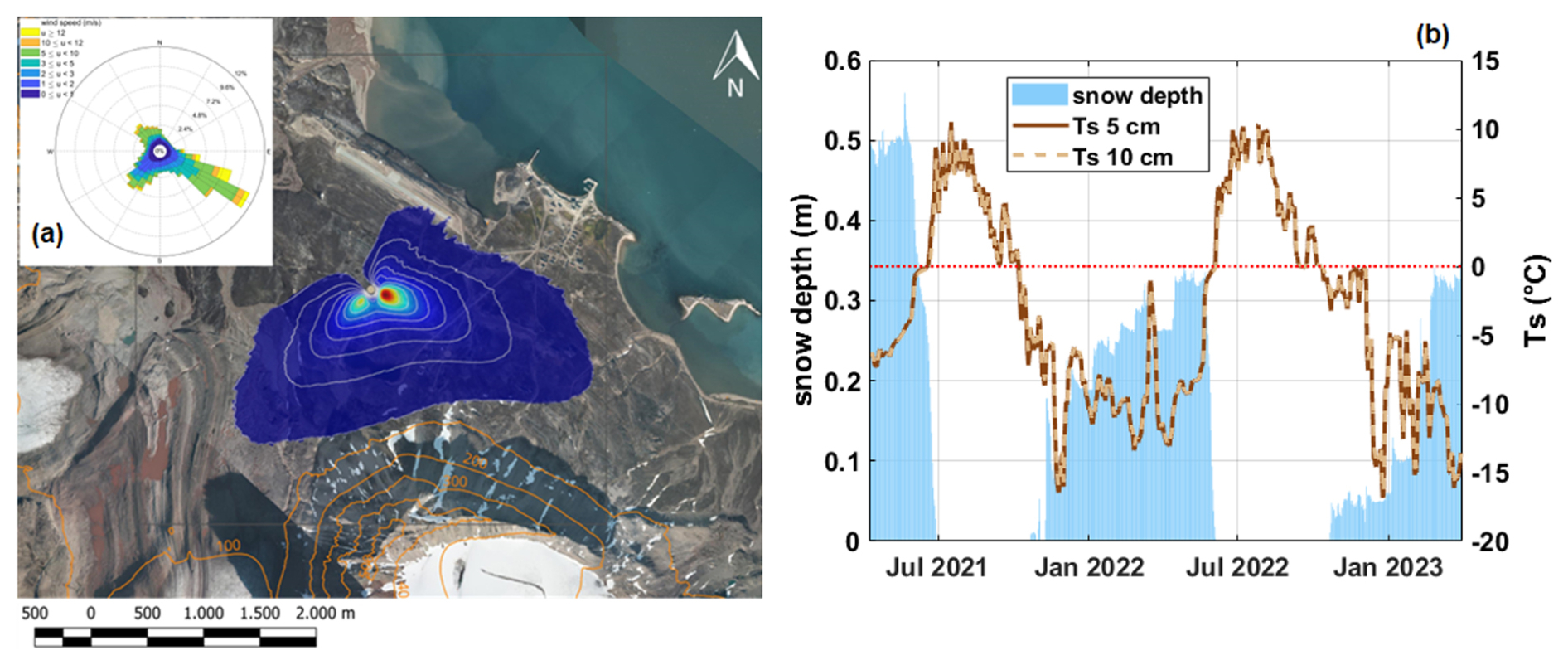
Figure 1 (a) Location map of the observation site: Ny Ålesund (Svalbard, Norway). The yellow point indicates the Amundsen–Nobile Climate Change Tower (CCT). © Norwegian Polar Institute, http://www.npolar.no (last access: 12 March 2024). In the figure the foreground of the flux footprint for the measurement setup is also reported (Sect. 2.3) at the 80 % contour line. In the inset the wind rose is reported for the period 2010–2023. (b) Soil temperature at two depths (5 and 10 cm) on the right axis and snow height (on the left axis) at the CCT site.

2 Methods

2.1 Measurement site

Methane and carbon dioxide turbulent fluxes were measured on the “Amundsen–Nobile Climate Change Tower” (CCT) (Mazzola et al., 2016), located north-west of the village of Ny Ålesund (78°55^′ N, 11°56^′ E) on Spitsbergen Island (Svalbard archipelago, Norway). The measurement campaign ran from 9 April 2021 to 31 March 2023, for a total of 2 years. The site is located on the top of a hill, and the land-cover during summer months is characterized by dry tundra or bare soil (Magnani et al., 2022). The climate is typically subarctic with a warming effect by the West Spitsbergen Ocean Current, a branch of the North Atlantic Current. The area is characterized by an average air temperature of about −10 °C in March and 6 °C in July, with about 400 mm of precipitation annually, falling mostly as snow between September and May (Lüers et al., 2014). The wind velocity average is 4.15 m s⁻¹, with a maximum monthly average of 5.47 m s⁻¹ in December and a minimum in August (2.9 m s⁻¹). Wind direction is essentially from three directions, with air masses coming from the south-east (42 %), south-west (27 %), and north–north-west (20 %) (see Fig. 1a, inset). A detailed description of the meteorological and micrometeorological conditions for the measurement period is reported, respectively, in Appendix B and Appendix C. The CCT area is a semi-desert ecosystem rather than wetland or heath tundra (Uchida et al., 2009). The vegetation cover at the measurement site (Fig. A1c) was estimated to be approximately 60 %, with the remainder being bare soil with a small proportion of stones (Lloyd et al., 2001; Boike et al., 2018).

The vegetated portion around and within the system footprint area consists of tundra, a widespread ecosystem in Svalbard (Magnani et al., 2022). Specifically, the vegetation is dominated by low-growing vascular plants. This includes various grass and sedge species, such as Carex spp., Deschampsia spp., Eriophorum spp., Festuca spp., and Luzula spp. Additionally, flowering plants like catchfly and saxifrage, as well as woody species like willow, are present. Notably, some locally common species like Dryas octopetala, Oxyria digyna, and Polygonum viviparum are also found (Fig. A1c). A moss and lichen layer is present, though the specific composition remains unclassified (Ohtsuka et al., 2006; Uchida et al., 2009; Lüers et al., 2014). In Ny Ålesund village, the thermal power plant for electricity production is the primary source of CO₂. On the other hand, there are a few combustion engine cars on the roads and some electric vehicles that might affect measurements occasionally. The village lacks specific combustion sources, relying entirely on electric facilities. The airport has only two flights per week, and ship arrivals are uncommon, occurring one to two times a month; however, cargo handling involves heavy-duty vehicles, and it is moderately active. All these activities are out of the measurement system footprint.

2.2 Instruments

Standard meteorological data such as air temperature (T) and relative humidity (RH), atmospheric pressure, and wind speed and direction were measured at different levels of the CCT (Fig. A1a) by means of the setup described in Mazzola et al. (2016). Snow depth at the foot at the CCT was measured with an ultrasonic range sensor (Campbell Scientific, model SR50A), while soil temperature (T_s) was recorded continuously using two temperature probes (Campbell Scientific, model 107) positioned at two different depths: 5 and 10 cm from the ground level. All sensors were connected to a data logger (Campbell Scientific, model CR-3000). Precipitation data for Ny Ålesund were downloaded from the Norwegian Centre for Climate Services web portal (https://seklima.met.no/observations/, last access: 18 March 2024). Radiation components (incoming and outgoing shortwave and longwave) were measured by means of a radiometer (CNR1; Kipp and Zonen, Netherlands) positioned at 33 m height above the ground with the sensor arm directed towards the south.

To measure the eddy covariance (EC) fluxes, a three-dimensional sonic anemometer (WindMaster Pro, Gill) and two open-path gas analysers (LI-7700 for methane and LI-7500 for water vapour and carbon dioxide, both from LI-COR Biogeosciences) were used. All data were recorded at 20 Hz using a SMART Flux interface unit (LI-7550, LI-COR Biogeosciences). The instruments were mounted at a height of 15 m on the CCT above the ground level. Figure A1b shows a typical instrument mounting on the horizontal bar. Air temperature, relative humidity, and pressure were also measured by the LI-COR system. The total data coverage during this experiment was 83 % for the anemometer, 78 % for the LI-7500, and 61 % for the LI-7700. During this measurement period, a longer break between 8 February and 3 March 2022 was registered in the dataset due to malfunctions in the eddy covariance system. Further, the measurements suffered a break period of 15 d from 5 to 20 February 2023 and stopped for 11 d in December 2022 and March 2023, respectively. Another break period in the dataset must also be included in June 2022 (from 13 to 23 June) for a total of 10 d. These periods comprise about 10 % of the whole dataset.

2.3 Eddy covariance data analysis

Eddy covariance (EC) vertical turbulent fluxes of GHGs were calculated on a 30 min average using the open-source software EddyPro^® package (version 7.0.3; Li-COR Biosciences, USA). The micrometeorological convention of assigning positive values to upward fluxes (emissions) and negative values to downward fluxes (towards the surface) was followed in this work. Spikes in the 20 Hz time series were removed from the dataset and replaced by linear interpolation of neighbouring values using a procedure described by Mauder et al. (2013). Data were discarded when the instrument measurement path became obstructed by water (rain, dew, or snow). Data corresponding to winds blowing from a 260–10° sector on the back of the EC setup were excluded from the analysis as they were in the wake of the tower structure (about 18 % on the whole dataset). In addition, the diagnostic values of the LI-7700 and LI-7500 gas analysers were used for data quality screening. For the CH₄ analyser, LI-7700, the relative signal strength indication (RSSI) was also considered. Methane fluxes were discarded if the mean RSSI of the respective averaging interval was <20. Spectral corrections were applied to the fluxes using the method described by Fratini et al. (2014). The high- and low-frequency spectral attenuations were both compensated for. The low-frequency loss due to finite averaging time and linear detrending was corrected following Moncrieff et al. (2004). The high-frequency loss due to path averaging, signal attenuation, and the finite time response of the instruments was taken into account following Massmann (2000, 2001). Spectral losses due to crosswind and vertical instrument separation were corrected following Horst and Lenschow (2009). Data at 30 min marked by spikes, drop-outs, discontinuities, or inputs outside absolute limits were discarded from the dataset. Specifically, all data outside of the 1st–99th percentile range were discarded from the subsequent analysis (about 1 % of data for each variable). The processing of the raw data included an angle-of-attack correction, i.e. compensation for the flow distortion induced by the anemometer frame (Nakai et al., 2006). To minimize the anemometer tilt error, a three-dimensional coordinate system transformation was applied to the dataset using the planar fit method proposed by Wilczak et al. (2001). This method ideally results in a null vertical wind component over a long period. The planar fit coefficients are calculated for the months of May (with snow) and August (with bare tundra) in the first and second year. The fit coefficients were calculated over the whole direction sector around the measurement site, spanning a 60° wind sector. A linear detrending procedure (Gash and Culf, 1996) was applied to the time series before the calculation of the 30 min average fluxes in order to remove the effects of low-frequency variations and instrument drifts. The Webb–Pearman–Leuning (WPL) correction was applied to compensate for the air density fluctuations, due to thermal expansion or water dilution, to the calculation of the fluxes (Webb et al., 1980; Burba et al., 2008). Further, a correction, considered in the so-called WPL+ module, was applied to consider the broadening of the spectroscopic line for CH₄ due to the contemporary presence of the water vapour (McDermitt et al., 2011). An important source of errors is the heat generated by the sensor body of the LI-7500 open-path gas analyser, which may generate convection within the sampling volume (Lafleur and Humphreys, 2007) impacting the calculations of the CO₂ fluxes measured by the LI-7500. The correction methods proposed by Burba et al. (2008) yield unrealistic flux values (with a large positive bias) for this dataset, especially during the winter season, so we chose not to apply this correction (Lüers et al., 2014). Finally, a negative CO₂ flux in the cold season can result from errors propagated through the density correction because the CO₂ density (ρ_c) can be affected by systematic biases caused by dirt contamination on the transducers and by the ageing of the optical components (Fratini et al., 2014). The bias in the CO₂ flux scales linearly with the sensible heat flux H if the CO₂ density is underestimated by a constant amount, causing the CO₂ flux to be too negative (Serrano-Ortiz et al., 2008). In theory, these two fluxes (CO₂ and H) should be independent of each other in cold conditions (T_air<0 °C) when photosynthesis is suppressed (Wang et al., 2017). Thus, the correction procedure reported in Wang et al. (2017) was applied to the CO₂ flux (with a mean slope of −0.0084 $\mathrm{\mu }\mathrm{mol}{\mathrm{m}}^{-\mathrm{2}}{\mathrm{s}}^{-\mathrm{1}}$ per W m⁻², R²=0.92). The detection limit (LOD) of the system was obtained using the method proposed by Finkelstein and Sims (2001). For CO₂ the LOD value result was on average 0.3 $\mathrm{\mu }\mathrm{mol}{\mathrm{m}}^{-\mathrm{2}}{\mathrm{s}}^{-\mathrm{1}}$, while for CH₄ it was 0.9 nmol m⁻² s⁻¹. In 16 % of the cases, exchange fluxes were lower than the calculated LOD, and by looking at the difference in the cumulated flux values, the contribution of these very low fluxes was 13 g C m⁻² (3 %) for CO₂ and 0.02 g C m⁻² (5 %) for CH₄: they were excluded from the final computation. However their inclusion would not have overturned the outcome. The 30 min fluxes underwent quality control based on atmospheric stability and developed turbulence as described by Mauder and Foken (2004). This method was applied to all flux values and classified the dataset into three groups: high-quality data (class 0), intermediate-quality data (class 1), and low-quality data (class 2 – discarded). Following this procedure, 6 % for the momentum flux; about 10 % for the CO₂, H₂O, and CH₄ flux; and 15 % for the sensible heat flux H were rejected. Some quality indicators derived from the raw data statistics as described by Vickers and Mahrt (1997) were also evaluated. Fluxes related to low-turbulence development conditions, i.e. not sufficient to guarantee suitable mixing, need to be identified and filtered out according to a friction velocity threshold (Aubinet et al., 2012). Such a value was computed (online tool available at https://www.bgc-jena.mpg.de/bgi/index.php/Services/REddyProcWeb, last access: 24 November 2023) using the bootstrapping approach described by Reichstein et al. (2005) and Papale et al. (2006). In our case, it provided $u^{*}=\mathrm{0.0497}$ m s⁻¹, and it was used to filter the dataset of the CO₂ and CH₄ fluxes, discarding all data corresponding to friction velocities lower than the threshold (0.8 % of the data).

The small gaps in the dataset, with durations less than 2 h, were filled by a linear regression (Lüers et al., 2014). Finally, the validated data (as a percentage of the total data point) used in this work add up to 63 % (21 845 points) for H, 48 % (16 649 points) for CO₂–H₂O flux, and 42 % (14 555) for CH₄ fluxes. Meteorological variables were gap-filled with ERA5 data. ERA5 is a reanalysis product from the European Centre for Medium-Range Weather Forecast that provides hourly estimates for various meteorological and soil variables starting from 1959 at a spatial resolution of 25 km (https://www.ecmwf.int/en/forecasts/datasets/reanalysis-datasets/era5, last access: 24 March 2024). Each variable was bias-corrected using a linear fit between ERA5 and flux tower observations during periods when both were available. The CO₂ and CH₄ fluxes time series, as said previously, showed some large gaps (up to 20 d for winter 2022); thus a gap-filling procedure has also been applied to these time series to avoid biases in the annual flux budgets. Gap filling for CO₂ fluxes was implemented, firstly, through the R package REddyProc (https://r-forge.r-project.org/projects/reddyproc/, last access: 10 March 2024; Reichstein et al., 2005). This gap-filling technique, based on marginal distribution sampling (MDS), used as input drivers the incoming shortwave radiation, air temperature, the soil temperature at 10 cm depth, relative humidity, and vapour pressure deficit. However, to take into consideration a large range of meteorological interactions and some biogeochemical variables, a random forest regression model of the fluxes was also developed (Kim et al., 2020; Knox et al., 2021) with 12 environmental drivers: sensible and latent heat fluxes, air temperature, soil temperature at 10 cm depth, relative humidity, vapour pressure deficit, air pressure, shortwave incoming and longwave outgoing radiation, the snow depth, the friction velocity, and finally the boundary layer height. Furthermore, the CO₂ flux (gap filled) was itself added as a driver for gap filling the CH₄ flux data. Only the gaps in the flux time series were filled with the resulting flux estimates from the random forest regression model. The implementation of the random forest model was developed with open-source Python libraries such as scikit-learn (Pedregosa et al., 2011). After a process of model tuning, the optimal values for various training parameters were found, such as the number of estimators (decision trees) and the maximum depth of the model. The training of the model and the model performance estimation were conducted following common methodologies as reported in Dyukarev (2023), which resulted in a validation error (normalized root mean squared error) of 7.75 % for the CO₂ and 9.37 % for the CH₄ inference.

The ratio between wind velocity and the friction velocity in neutral atmosphere ($-\mathrm{0.05}<z/L<\mathrm{0.005}$, where z is the measurement height and L is the Obukhov length) was used to evaluate the average roughness length z₀ for the site analysed using a parameterization based on similarity theory (Stull, 1988). The results gave $z_{\mathrm{0}}=\mathrm{0.005}\pm \mathrm{0.001}$ m, with similar results reported also by Mazzola et al. (2021) and Donateo et al. (2023) at the same site. Separating the winter period (with snow coverage) from the summer period (without snow), z₀ values were calculated as $z_{\mathrm{0}}=\mathrm{0.002}\pm \mathrm{0.001}$ m (winter) and $z_{\mathrm{0}}=\mathrm{0.004}\pm \mathrm{0.001}$ m (summer). A null displacement height d was considered for this site as obstacles of significant height are not present around the site and in its footprint. Source areas for scalar fluxes have been evaluated using a Lagrangian footprint model proposed by Kljun et al. (2015). The results of flux footprint analysis are shown in Fig. 1 with the different influence levels of the zones on the measurements. The gas fluxes measured represented a surface area of about 2.4 km² (considering the 80 % contour line) with a maximum distance of 1300 and 1600 m in a south-west and a south-east direction, respectively. It is worth remembering that the data in the wake of the tower structure to the north-west and north-east were excluded from the analysis. The flux peak contribution was in the wind direction sectors at about 130 m (±5 m) to the south-east and south-west (Fig. 1). However, the source land area was very similar for the considered wind direction sectors around the measurement site, with 100 % of snow coverage for the winter period. During the summer period the footprint area was over tundra coverage, with about 2.4 % covered by water surfaces (two arctic lakes) (Fig. 1).

2.4 Seasonality

In this work the calendar year was divided into a snow-covered season (winter); a snow-free season (summer); and thawing and freezing periods in late spring and autumn, respectively. Thawing period represents a transitional phase during which the snow cover melts. Daily soil temperature and snow depth were used to define the different seasons. The start of the snow-covered season was defined as the start of the freeze-up, i.e. the first day on which daily mean T_s at 5 cm depth is below −0.75 °C for 3 consecutive days (Oechel et al., 2014; Taylor et al., 2018; Arndt et al., 2019; Bao et al., 2021) and at the same time daily snow depth is greater than 1 cm. The end of the snow-covered season was defined as the start of thaw, i.e. the first date on which daily mean T_s at 5 cm depth rose above 0.75 °C for at least 3 consecutive days. The winter season was between the end of the freezing period (the total solar radiation being <10 W m⁻²) and the beginning of the thawing period. At the same time the summer season was defined as the period between the end of thawing (the snow depth being lower than 1 cm) and the beginning of the freezing period. Thawing and freezing periods are also called in the paper “shoulder seasons”, as reported by Bao et al. (2021). Further, the winter season was divided into a first period (dark winter) with an absence of solar radiation (total radiation <10 W m⁻²) and a second one (light winter) with an increasing total radiation greater than 10 W m⁻². Thereby two complete light winter (snow-covered) seasons during the study period could be defined: from 1 March 2022 to 19 May 2022 (80 d) and from 5 to 31 March 2023 (27 d). Furthermore, an initial period from 9 April 2021 to 27 May 2021 (48 d) has also been included as a snow-covered period. Two dark winter periods (snow-covered), as specified earlier without solar radiation, have been identified: from 23 October 2021 to 28 February 2022 (128 d) and from 23 October 2022 to 4 March 2023 (132 d). Two complete summer seasons were also included in the dataset: from 29 June 2021 to 7 October 2021 (100 d) and from 4 June 2022 to 13 October 2022 (131 d). Finally, two thawing and freezing periods in 2021 and 2022 were covered in this work: specifically thawing in the months of May and June and freezing in the month of October for a total thawing period of 45 d and freezing period of 22 d.

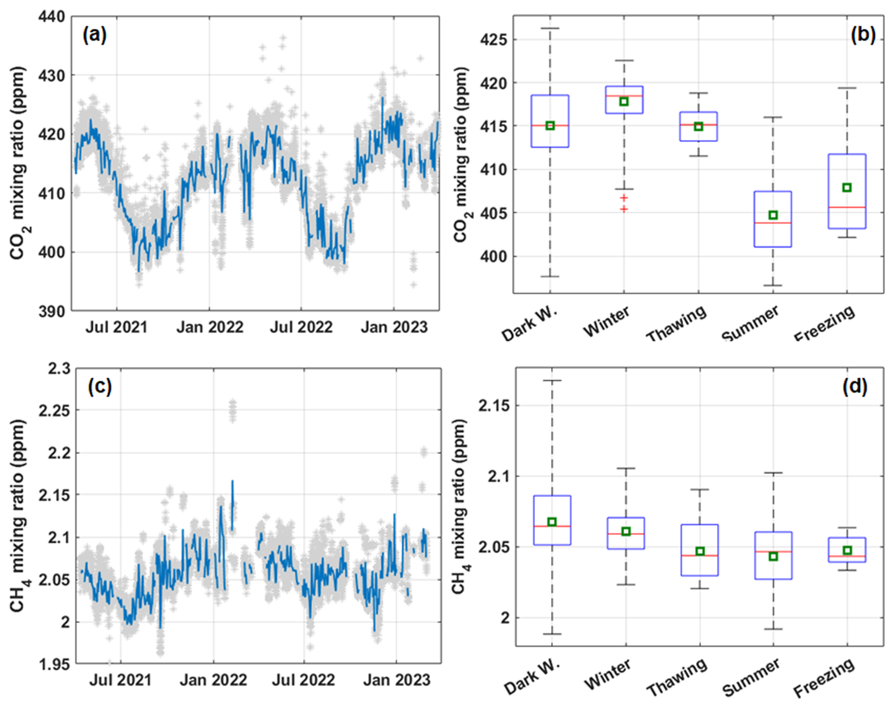
Figure 2 Time series on a daily basis (a, c) and whisker–box plots (b, d) of (a, b) CO₂ and (c, d) CH₄ mixing ratios. In the left panels, in light grey are the time series for CO₂ and CH₄ mixing ratio at 30 min resolution. In the right panels, whiskers represent max and min values, and the box limits are the 25th and 75th percentiles. The red line represents the median value on a 30 min basis.

3 Results and discussion

3.1 CO₂ and CH₄ mixing ratio and surface fluxes

Median CO₂ mixing ratio over the whole measurement period was 413.66 ppm (average 412.30 ppm) with an interquartile range (IQR 25th–75th percentile) from 406.17 to 417.72 ppm (Fig. 2a). The CO₂ mixing ratio was greater during the winter period with a median value of 418.46 ppm decreasing towards the summer season, when it measured a median of 403.81 ppm with a minimum value of 396.61 ppm (Fig. 2b). The shoulder season was characterized by an intermediate CO₂ concentration: the thawing season showed a median mixing ratio of 415.14 ppm, greater than the CO₂ concentration in the freezing season (405.62 ppm) (Fig. 2b). The median CH₄ mixing ratio for the measurement period was 2.05 ppm (IQR 2.04–2.07 ppm) (Fig. 2c). In this case, the greatest concentration was found during the dark winter season (2.06 ppm) with a decreasing trend going towards the summer season down to a median value of 2.05 ppm. The thawing and freezing seasons presented very similar values in CH₄ concentration: 2.044 and 2.043 ppm, respectively (Fig. 2d).

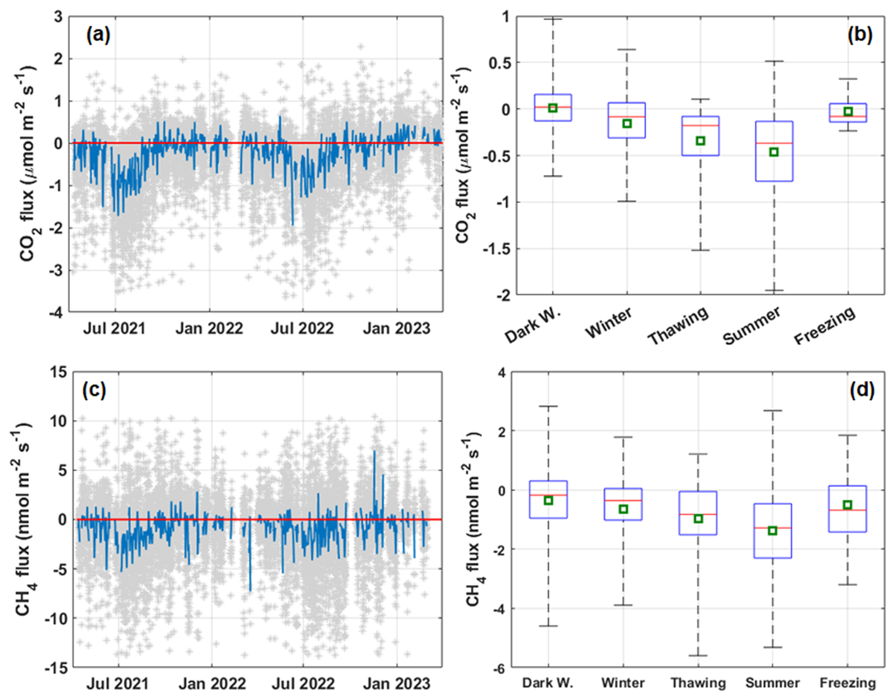
Figure 3 Time series on a daily basis (a, c) and whisker–box plots (b, d) of turbulent vertical flux (a, b) CO₂ and (c, d) CH₄ measured at the CCT site. In the left panels, in light grey are the time series for CO₂ and CH₄ mole fraction at 30 min resolution, and the red line represents the zero level for fluxes. In the right panels, whiskers represent max and min values, and the box limits are the 25th and 75th percentiles. The red line represents the median value and the green square the average value.

In Fig. 3a and c, the annual cycle of CO₂ and CH₄ turbulent fluxes was observed, with CO₂ and CH₄ fluxes exhibiting negative intensity for the greater part of the year. The CO₂ flux had a median value for the whole period of −0.032 $\mathrm{\mu }\mathrm{mol}{\mathrm{m}}^{-\mathrm{2}}{\mathrm{s}}^{-\mathrm{1}}$ (detailed statistics in Table 1). At the same time, the median value for the CH₄ flux was −0.39 nmol m⁻² s⁻¹ (Table 1). Negative values are particularly important in CO₂ and CH₄ fluxes during the summer season (growing season), indicating a sink behaviour for the CCT site.

Table 1 Statistical analysis for the CO₂ and CH₄ fluxes at the measurement site separated into five different seasons defined in this work.

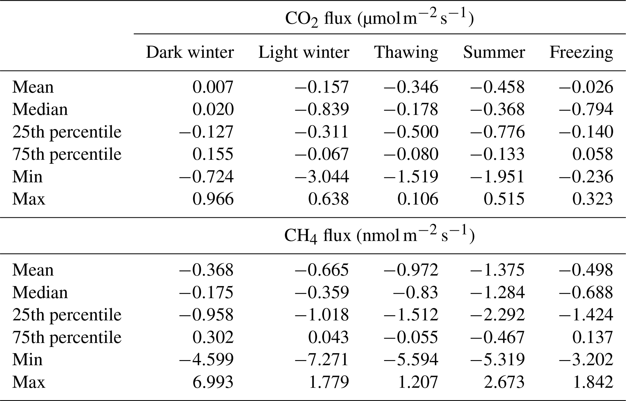
Seasonal analysis revealed negative median values for the fluxes of CO₂, peaking in summer at −0.37 $\mathrm{\mu }\mathrm{mol}{\mathrm{m}}^{-\mathrm{2}}{\mathrm{s}}^{-\mathrm{1}}$. The CO₂ fluxes showed a slightly positive median value during the dark winter (0.02 $\mathrm{\mu }\mathrm{mol}{\mathrm{m}}^{-\mathrm{2}}{\mathrm{s}}^{-\mathrm{1}}$), actually due to respiration phenomena from the snow-covered surface due to microbial respiration (Hicks Pries et al., 2013). At a finer timescale (30 min resolution), the CO₂ flux trend indicated the presence of positive fluxes (emissions) (Fig. 3a), especially during the dark and light winter and the freezing period (Table 1). As snowmelt begins, accumulated carbon dioxide may be released and exposed patches of ground with a lower albedo begin to warm, further enhancing respiration rates and CO₂. Further, during thawing season, incoming radiation reaches levels adequate for photosynthesis: the combination of increasing light, along with increases in soil temperatures, can result in early photosynthesis. At the CCT site, the CO₂ flux decreased starting from the light winter (−0.84 $\mathrm{\mu }\mathrm{mol}{\mathrm{m}}^{-\mathrm{2}}{\mathrm{s}}^{-\mathrm{1}}$) and continues during the thawing season (−0.18 $\mathrm{\mu }\mathrm{mol}{\mathrm{m}}^{-\mathrm{2}}{\mathrm{s}}^{-\mathrm{1}}$). During the autumn, soil temperatures were still adequate for substantial microbial respiration. When the senescence of vascular plants advanced, respiration became the dominant process affecting carbon exchange. In addition, as soils freeze, CO₂ may be forced out of the soil towards the atmosphere. However, in the freezing period, at the CCT site, a median negative CO₂ flux has been measured (−0.79 $\mathrm{\mu }\mathrm{mol}{\mathrm{m}}^{-\mathrm{2}}{\mathrm{s}}^{-\mathrm{1}}$).

A similar trend is reported for methane: during the dark and light winter periods, methane fluxes are negative, with a median value of −0.17 and −0.36 nmol m⁻² s⁻¹, respectively (Fig. 3d). Treat et al. (2018) investigated methane dynamics across Arctic sites and reported negative methane fluxes during winter, attributed to cold temperatures which inhibit methanogenesis while promoting methane oxidation in dry tundra soils. However, they also highlight methane uptake in dry tundra during colder periods. Zona et al. (2016) reported that methane emissions during the cold season (September to May) account for ≥50 % of the annual CH₄ flux, with the highest emissions from upland tundra. In this study (Table 1), evidence of significant emission events during winter temperature fluctuations can be observed at the site. In contrast, these events diminished in the shoulder seasons, when notable net uptake events dominated at −0.83 nmol m⁻² s⁻¹ during the thawing period and −0.69 nmol m⁻² s⁻¹ during the freezing period. Seasonal analysis revealed negative median CH₄ fluxes, peaking in summer at −1.28 nmol m⁻² s⁻¹. Juncher Jørgensen et al. (2015) field measurements, within the Zackenberg Valley in north-east Greenland over a full growing season, showed methane uptake with a seasonal average of −2.3 nmol CH₄ m⁻² s⁻¹ in dry tundra. Wagner et al. (2019) measured a negative peak during the growing season (2009) of −4.41 ng C–CH₄ m⁻² s⁻¹ in a polar desert area at the Cape Bounty Arctic Watershed Observatory (CBAWO; Melville Island, Canada).

Even though a similarity between the CO₂ and CH₄ flux patterns can be observed from the time series, the exchange processes are probably led by different physical drivers. Significantly negative fluxes of CO₂ are driven by photosynthesis, while CH₄ uptake fluxes increase, coinciding with a positive peak in ground temperatures (Mastepanov et al., 2013; Howard et al., 2020). While prior research demonstrated the influence of soil temperature on methanotrophic activity (Reay et al., 2007), CH₄ fluxes at the CCT site showed limited response to soil temperature, as reported later.

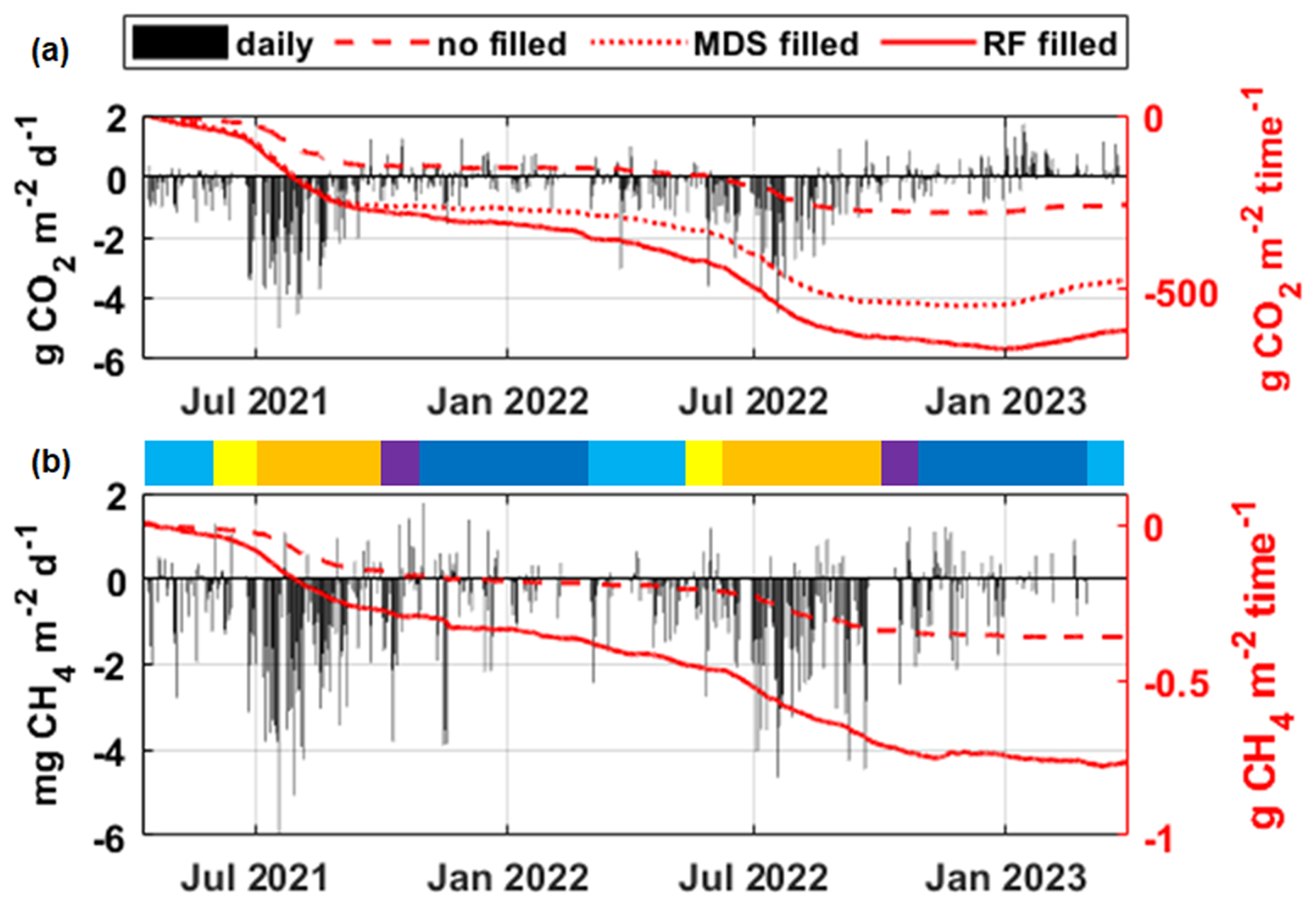
Figure 4 Daily (black bars – left axis) and mass cumulative (red – right axis) ecosystem exchange for (a) CO₂ and (b) CH₄ measured at the CCT site. Mass cumulative exchange for CO₂ and CH₄ was reported: dashed line for no gap-filled time series, dotted line for MDS, and continuous line for RF. Central multicoloured bar separates the time series into five different seasons: blue for light winter, yellow for thawing, orange for summer, purple for freezing, and navy for dark winter.

3.2 CO₂ and CH₄ mass budget

The cumulative mass budgets over the 2 monitoring years in the ecosystem of the CCT site are shown in Fig. 4. Based on the budget for the whole measurement period, the study area acts as a net sink for both CO₂ and CH₄. During the study period, a CO₂ balance of almost −257 CO₂ g m⁻² is found, while the contribution of CH₄ uptake was estimated at approximately −0.36 g CH₄ m⁻² (Fig. 4, dashed red line). Actually, for the evaluation of the cumulated carbon, the gap-filled time series should be considered (with both MDS and random forest (RF) methodology; see Sect. 2.3). In this perspective, the total cumulative CO₂ budget over the measurement campaign was −472 g CO₂ m⁻² with MDS and −650 g CO₂ m⁻² using the RF procedure (Fig. 4a). On the other hand, CH₄ cumulative budget was about −0.76 g CH₄ m⁻² with the RF gap-filling procedure (Fig. 4b). The mean annual cumulative CO₂ budget was −131 g CO₂ m⁻² with MDS and −164 g CO₂ m⁻² with RF. Oechel et al. (2014) reported a net CO₂ uptake during the summer season of −24.3 g C m⁻², while the non-growing seasons released 37.9 g C m⁻², showing that these periods include a significant source of carbon to the atmosphere. In Treat et al. (2024) for 2002–2014, a smaller CO₂ sink in Alaska, the Canadian tundra, and the Siberian tundra is reported (medians: −5 to −9 g C m⁻² yr⁻¹). Euskirchen et al. (2012) established eddy covariance flux towers in an Alaska heath tundra ecosystem to collect CO₂ flux data continuously for over 3 years. They measured a peak CO₂ uptake during July, with an accumulation of −51 to 95 g C m⁻² during June–August. On average, the mean annual cumulative budget for CH₄ was −0.18 g CH₄ m⁻² yr⁻¹, calculated using gap-filled data (Table 2). This outcome lies within the same order of magnitude estimated by Dutaur and Verchot (2007) at the global level, reporting a net CH₄ uptake for the non-forested arctic environments (defined as “boreal other”) of −0.14 g CH₄ m⁻² yr⁻¹. Treat et al. (2018) found that tundra upland varies from CH₄ sink to source with a median annual value of 0.0±0.20 g C m⁻² yr⁻¹. Lau et al. (2015) found that the CH₄ uptake rate was in the range between −0.1 and −0.8 mg CH₄–C m⁻² d⁻¹ at the AHI site (Nunavut, Canada). In this work it was suggested that mineral Cryosols act as a constant active atmospheric CH₄ sink (Emmerton et al., 2014) in part because of their low soil organic carbon availability, low vegetation cover, and low moisture content.

Table 2 Mean mass cumulative grams of CO₂ and milligrams of CH₄ for each season defined in this work and the mean cumulated grams of CO₂ and milligrams of CH₄ yearly at the measurement site. The values are reported for the original gap time series (RAW), the gap-filled dataset with MDS, and the RF procedure.

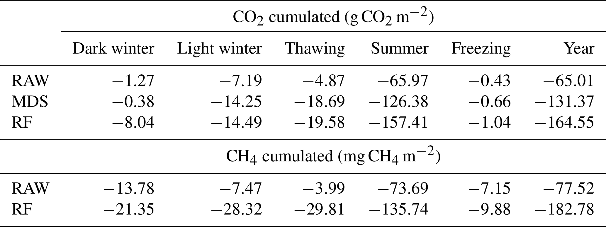
The annual budget can be further split into the five seasons considered in this study. Specifically, the CCT area acted as a CO₂ sink during the thawing and summer period with an average value of −0.79 and −1.1 g CO₂ m⁻² d⁻¹, respectively. During the freezing period the quantity of absorbed CO₂ per day decreased down to almost null value (−0.01 g CO₂ m⁻² d⁻¹) and slightly increased to a positive value during the dark winter period (0.04 g CO₂ m⁻² d⁻¹). With the increasing amount of the solar radiation, the mass cumulative CO₂ per day decreased again (−0.25 g CO₂ m⁻² d⁻¹ for light winter). Ueyama et al. (2014) analysed seasonal CO₂ budgets across several tundra ecosystems in Alaska, reporting peak CO₂ uptake during summer with an average value of −46 g C m⁻² due to maximum photosynthesis rates. The same pattern was followed by the CH₄ absorbed carbon mass: in this case during the thawing period a value on average of −0.55 mg CH₄ m⁻² d⁻¹ was observed, its negative maximum peaking during the summer period (−1.29 mg CH₄ m⁻² d⁻¹). Also, in this case the absorbed carbon mass decreased in the freezing period down to −0.63 mg CH₄ m⁻² d⁻¹. It was reduced to very low values during the winter season at −0.26 mg CH₄ m⁻² d⁻¹ in dark winter and −0.40 mg CH₄ m⁻² d⁻¹ in light winter. Non-growing-season emissions accounted for 58 % of the annual CH₄ budget, characterized by large pulse emissions.

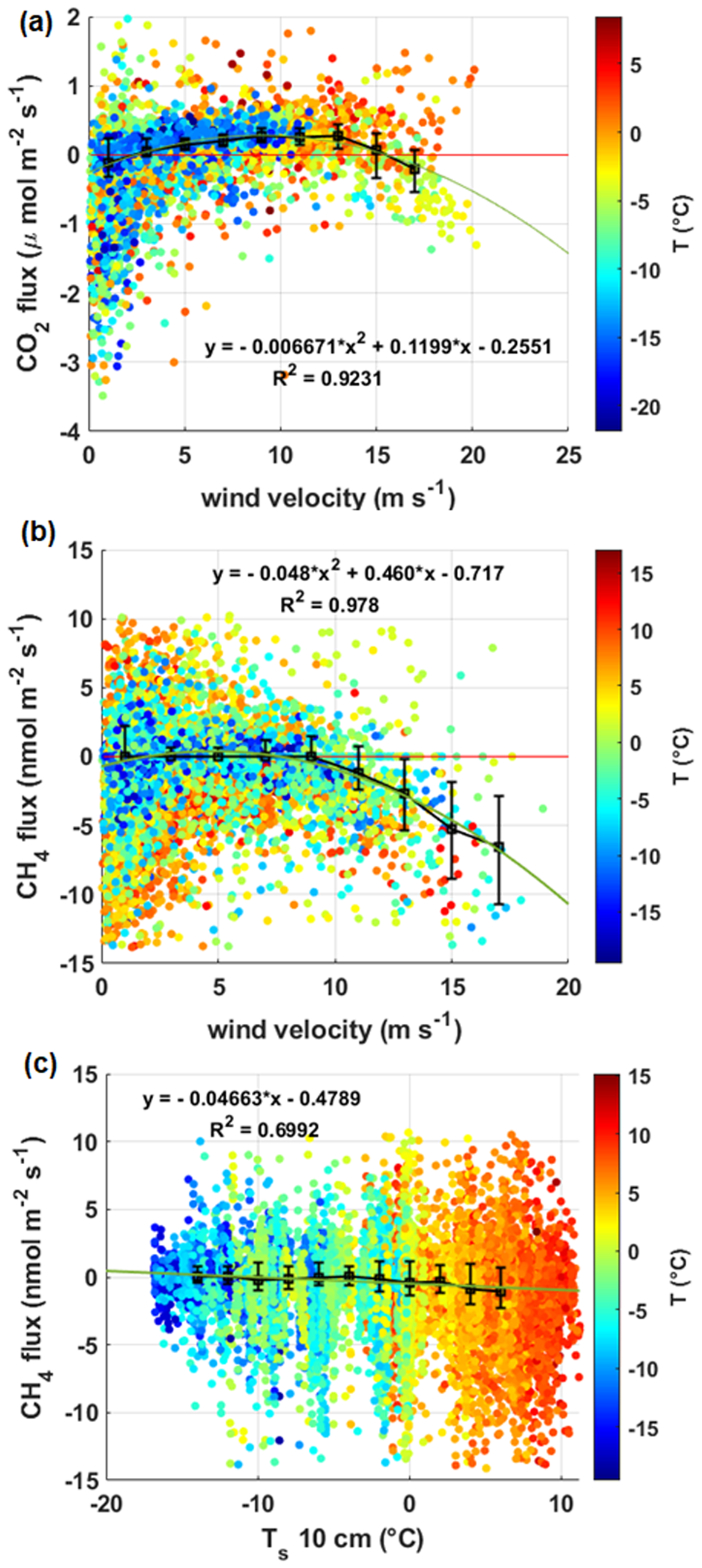
Figure 5 Scatter plot of turbulent vertical (a) CO₂ and (b) flux against wind speed. In (a) data were selected for the snow-covered period (dark and light winter). (c) Scatter plot of the vertical CH₄ flux as a function of the soil temperature T_s. Data in the panels are colour-coded according to air temperature T.

3.3 Physical drivers on GHGs surface fluxes

High-temporal-resolution measurements of CO₂ and CH₄ facilitate looking at the underlying causes of emissions, looking, for example, at the relationship between meteorological/flux variables and CH₄ fluxes (Taylor et al., 2018). Further, the importance of soil net CH₄ uptake is poorly constrained, but it is widely recognized that soil temperature, soil moisture, and substrate availability (CH₄ and O₂) are the main drivers of the temporal variations in observed and predicted net CH₄ fluxes (D'Imperio et al., 2023). Juncher Jørgensen et al.'s (2024) incubation studies revealed that subsurface CH₄ oxidation is the main driver of net surface–atmosphere exchange, and it responds clearly to changes to soil moisture in these dry upland environments. The production, consumption, and transport processes of CH₄ are primarily related to hydrology, vegetation, and microbial activities (Vaughn et al., 2016; Wang et al., 2022). In this work soil hydrology measurements are available for understanding these processes; however the measured wind velocity and soil temperature have been used as proxies for soil moisture and water table depth. Previous works have shown that advection, forced by wind pumping related to atmospheric turbulence, can increase turbulent fluxes from/to the snowpack (Sievers et al., 2015). Typically, the wind pumping effect led to increased emissions flux in CO₂ resulting from ebullition and/or ventilation. This correlation was analysed for the snow-covered periods (dark and light winter) at our measurement site (Fig. 5a). The scatter plot in Fig. 5a shows a quadratic relationship (the equation of the fit is reported in the figure, R²=0.91) between wind speed and vertical turbulent CO₂ flux, with a clear increasing trend indicating positive fluxes for wind speed above 3 m s⁻¹. From a similar analysis, but in this case for the whole measurement period, for the CH₄ fluxes (Fig. 5b), a quadratic relationship with the wind velocity (R²=0.98) can be observed in this case too. In the range of low-wind-velocity CH₄ exchange balance is on median values very close to zero, but going to greater wind speed (>10 m s⁻¹) the negative CH₄ flux (uptake) increases.

At the CCT site, where uptake seems to outweigh emission within the flux footprint, the soil layer would be relatively depleted in methane compared to the atmospheric boundary layer. The coarse soils at CCT may therefore experience increased aeration, which could in turn aid in the transportation of CH₄-rich air from the overlying atmosphere to the methanotrophs and/or enhance the movement of CH₄-depleted air from the soil into the atmosphere. In addition, increased aeration would provide oxygen to the deeper soil layers during the dry season, stimulating the activity of aerobic methanotrophs. Analysis through a scatter plot (Fig. 5c) depicting CH₄ flux alongside both soil and air temperature revealed a minimal correlation, indicating that variations in temperature had minimal impact on CH₄ fluxes. The extent to which temperature fluctuations affect CH₄ fluxes in the soil is heavily contingent on the depth of the microbial community responsible for these fluxes. Despite previous findings indicating that methanotroph habitats are typically situated near the soil surface at depths ranging from 3 to 15 cm (Curry, 2007; Yun et al., 2023), there was no assessment of the vertical distribution of microbial populations in the soil at the CCT site. Overall, the observed correlation in the ecosystem uptake of methane with wind velocity suggests that the methanotrophic communities in the Svalbard soils might be stimulated by soil aeration, strongly related to its drying out during the summer. Since the CCT is also a semi-desert surface, the CH₄ uptake regulation is most directly related to the porosity and soil hydrology (not measured in this study), indirectly affected by the wind that can dry the soil and increase diffusivity for atmospheric oxygen.

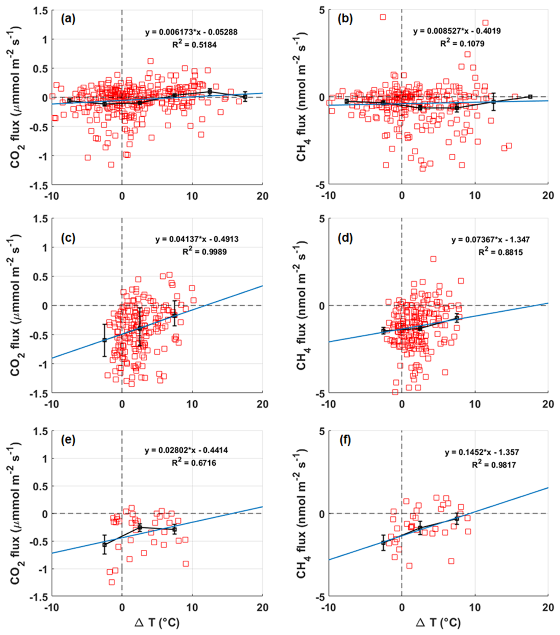
Figure 6 CO₂ vertical fluxes against temperature anomalies for (a) the whole winter (dark plus light winter), (c) the summer, and (e) the thawing season. CH₄ vertical fluxes against temperature anomalies for (b) the whole winter, (d) the summer, and (f) the thawing season. A linear fit of the data is reported with a green line. Black squares represent the flux data binned for ΔT bins (5 °C large). Error bars represent the standard errors.

3.4 GHG fluxes' response to seasonal temperature anomalies

In this work the seasonal temperature anomalies were evaluated as possible drivers for the modifications in GHG turbulent flux exchanges on a daily basis. This approach allowed for a comprehensive understanding of the relationship between thermal variations and corresponding flux dynamics over the considered period. In this study, the temperature anomalies were calculated with respect to the day-of-the-year average values, taking the period 1991–2020 as a baseline. Figure 6 depicts the dependence of the CO₂ and CH₄ turbulent fluxes on the temperature anomalies, on a daily basis, based on a 5 d running window. As can be observed, net uptake fluxes for both gases are most noticeable in conditions of above-zero ground temperatures, clearly indicating the summer period, but with thermal anomalies below 5 °C (Fig. 6c, d). The magnitude of uptake-gas flux decreases with increasing positive thermal anomalies during the summer (0.04 $\mathrm{\mu }\mathrm{mol}{\mathrm{m}}^{-\mathrm{2}}{\mathrm{s}}^{-\mathrm{1}}\mathrm{°}\mathrm{C}$ for the CO₂ and 0.07 nmol m⁻² s⁻¹ °C for the CH₄) until it reverses to a positive (emissive) flux, with an attenuated net uptake, for marked positive anomalies above 8 °C (Fig. 6a, b). This behaviour suggests that the trend is towards a null annual net uptake of CO₂, considering the increasing frequency and intensity of positive temperature anomalies. During the winter season, dark and light winter together, the gas fluxes did not show a particular trend against the thermal anomalies, with an average rate of about 0.006 $\mathrm{\mu }\mathrm{mol}{\mathrm{m}}^{-\mathrm{2}}{\mathrm{s}}^{-\mathrm{1}}$ °C for the CO₂ and 0.008 nmol m⁻² s⁻¹ °C for the CH₄ (Fig. 6a, b). Shoulder seasons show a positive trend between fluxes and thermal anomalies, albeit based on a tight range of thermal anomalies. Specifically, during the freezing season, uptake and emission fluxes occur with negative and positive anomalies, respectively (not shown here), with no specific trend. Figure 6e and f show the same type of analysis for CO₂ and CH₄ fluxes during the thawing season, which presents a consistent uptake for both positive temperature anomalies (below 10 °C) and also negative anomalies (above −5 °C). In the context of climate change, large positive anomalies could lead to positive (or at least null) fluxes in all seasons, while optimal situations could occur during the summer, considering a lower temperature increase in this season (Bintanja and Linden, 2013). Overall, the results suggest a transition of CO₂ and CH₄ flux regimes to an emissive scenario (reduced net uptake) for thermal anomalies above 10 °C for all the periods considered, especially for the winter, where the thermal anomalies have a greater relative magnitude. The findings in this study align with the observed decrease in the net carbon reservoir in northern ecosystems as air temperature rises (Cahoon et al., 2012; Zona et al., 2022). This suggests that future increases in temperature will weaken the ecosystem CO₂ sink strength or even turn it into a CO₂ source, depending on possible changes in vegetation structure and growing season length extension as a response to a changing climate (Lund et al., 2012; Ueyama et al., 2014).

4 Conclusions

In this study, CO₂ and CH₄ turbulent fluxes in tundra ecosystems on the Svalbard islands (Norway) were investigated, using a 2-year measurement campaign. The observed uptake and emission patterns in both CO₂ and CH₄ underscore the dynamic interplay between climatic conditions and ecosystem activities (such as photosynthesis and microbial activity) at the measurement site. During the summer season, the pronounced uptake flux (for both carbon dioxide and methane) suggests an increase in moss and lichen photosynthesis and/or microbial methane consumption, while the transition to neutral or null fluxes in the freezing season and in winter indicates a decrease in these activities. The enhanced methane uptake during the melting period aligns with the activation of soil microorganisms and correlates with the increasing aeration (wind effect) of the topsoil and its decreasing albedo. The CO₂ uptake intensified in the summer season, while during October the decreasing photosynthetic activity, together with the first occurrence of the snow, led to a sensible reduction in absorbing phenomena giving way to the ecosystem respiration and relatively low positive (or almost null) CO₂ fluxes. During the winter period the processes forcing CO₂ accumulation and CO₂ release counterbalance each other, resulting in very low positive fluxes. Given the nature of the mineral-rich soils of the investigated area and of a large portion of the Arctic ecosystem, methane oxidation by aerobic methanotrophs in this kind of soil plays an important role in reducing the methane net emission to the atmosphere. The methane budget shows a sink behaviour for this site, especially for the summer season gradually approaching neutral during the freezing season. The methane uptake decreases during the winter season due to the presence of the snow, and the methanotrophic activity is nearly stopped by negative soil temperature, which triggers the freezing process of the active layer water content. The methane uptake rate rises again during the melting period started by the activation of soil methanotrophic microorganisms. The CH₄ fluxes at CCT exhibited a limited association with both soil and ambient temperature in contrast to other environmental factors, such as the soil moisture and water table depth. In this work soil hydrology measurements are available for understanding these processes; however the measured wind velocity and soil temperature have been used as proxies for soil moisture and water table depth. Solar radiation and wind play a role in the speed of drying, but the soil material and structure ultimately determine how much it dries under the given climatic conditions. Overall, the observed correlation in the ecosystem uptake of methane with wind velocity suggests that the methanotrophic communities in the Svalbard soils are stimulated by oxygen uptake, strongly related to its drying out during the summer.

The analysis of the impact of thermal anomalies on CO₂ and CH₄ exchange fluxes, underscores that high positive (>5 °C) thermal anomalies may contribute to an increased positive flux in both summer and winter periods, effectively reducing the net annual uptake. Warming in permafrost ecosystems leads to increased plant and soil respiration that is initially compensated for by an increased net primary productivity. However, future increases in soil respiration will likely outpace productivity, resulting in a positive feedback to climate change (Hicks Pries et al., 2013). In both cases, for methane and carbon dioxide, the uptake fluxes are generally observed for moderate positive anomalies (<5 °C), especially during summertime. The implications of these results contribute valuable insights to our understanding of ecosystem responses in the face of evolving climatic conditions. If this trend is applicable also to other Arctic ecosystems, it will have implications for our current understanding of Arctic ecosystem dynamics. Further research is needed to better understand the sources and sinks of these GHGs in the dry upland tundra in order to develop effective references for models examining the dynamics of these ecosystems in response to climate change at local and global scale.

Appendix A: Climate Change Tower (CCT)

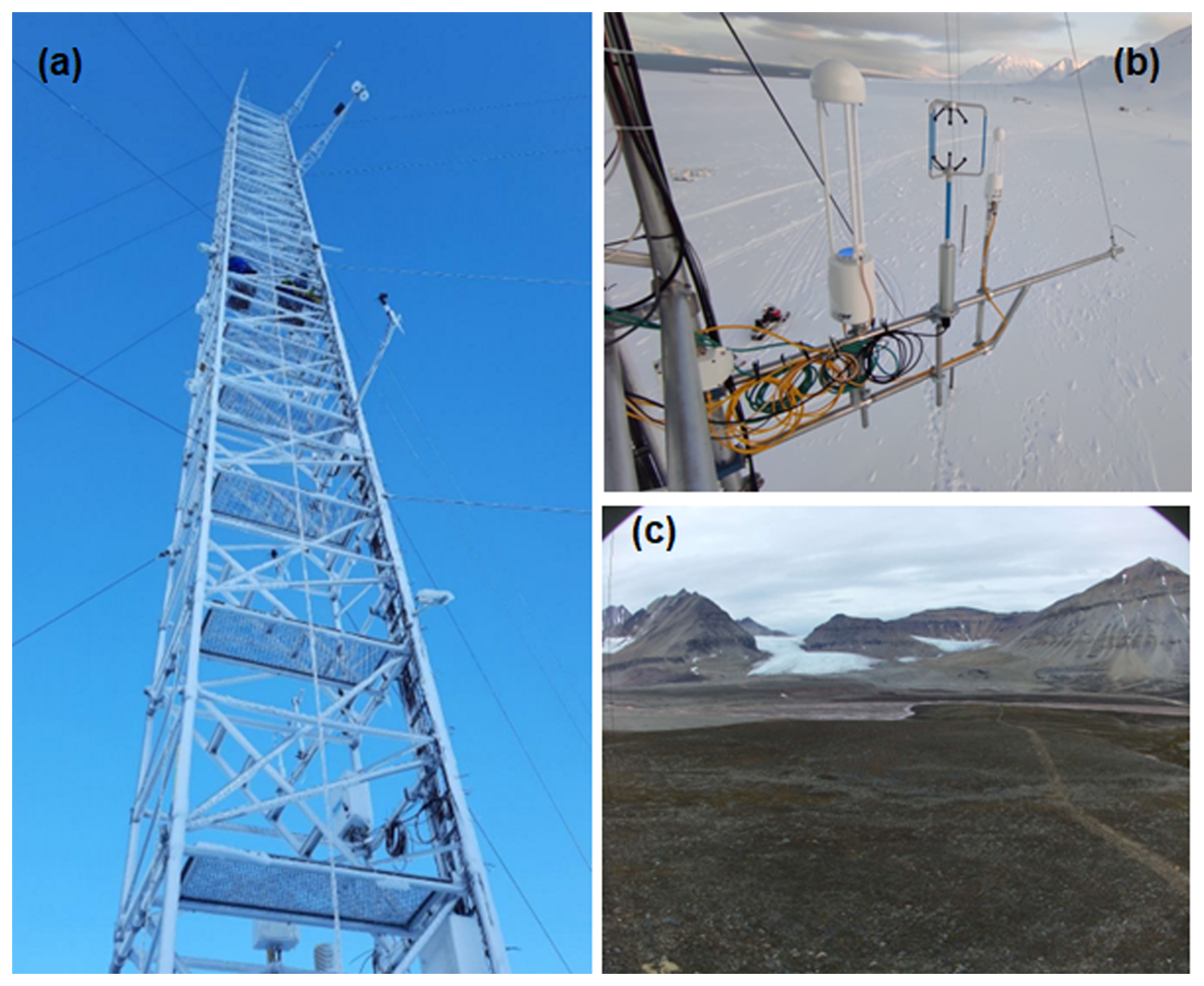
Figure A1 (a) Amundsen–Nobile Climate Change Tower (CCT) picture with instrumentation installed at different heights. (b) A picture of the EC installation setup with LI-7700 (left), sonic anemometer (middle), and LI-7500 (right) on the horizontal steel bar. (c) A bird's-eye view of the tundra at the CCT site. Photo courtesy of Roberto Salzano (CNR-IIA).

Appendix B: Meteorology at CCT for the measurement period

The mean air temperature was −1.3 °C (±7 SD) during the measurement period. March records the lowest T, with a daily average of −20.3 °C (see Fig. B1a), while from April onwards, T gradually rises, peaking at 13.5 °C daily in July. At the same time, RH reached its maximum value of 93 %, maintaining high levels throughout August (Fig. B1c). The minimum RH value of 31 % (on a daily basis) was recorded in April. Solar radiation (both global and net radiation) takes on positive values greater than 10 W m⁻² from the month of February (starting halfway through) until the month of October (to about the 15th) (Fig. B1e). The total precipitation in the area for the 2-year period was distributed as 235 mm in 2021 (from April to December), 573 mm in 2022, and 160 mm in 2023 (January–March only). Total solar radiation (downward shortwave radiation), which is one of the main drivers for the photosynthesis processes, showed relatively high median values for the thawing and winter seasons (510 and 332 W m⁻², respectively) and decreasing values for summer (392 W m⁻²) and freezing (240 W m⁻²) (Fig. B1e). Note that during dark winter the global radiation is very low, actually null, as this period has been defined. Snowpack in the first period until 27 May 2021 had an average depth of 0.41 m with a maximum peak at 0.56 m in 2021. In 2022 and 2023 the depth of the snowpack was lower, with an average depth of 0.24 and 0.14 m, respectively (Fig. 1b). The maximum snowpack depth in the last 2 years was 0.35 m. The snow is largely spread by wind, as is typical of such areas on Svalbard (Winther et al., 2003). Overall, the ground was covered by snow for 62 % of the measurement period. The average difference between T_s at 5 cm and T_s at 10 cm was 0.006 °C, with an absolute average gradient over the whole period of 0.12 °C m⁻¹ (Fig. 1b). The maximum T_s was 15 °C (in July) and the minimum −16 °C (in December 2022). In this work a particular focus was placed on the study of both shoulder seasons and winter and summer seasons. The temperature differences between the selected seasons were significant. Specifically, the winter period T (Fig. B1b) was sharply below zero (median −6.51 °C). The lowest cumulative precipitation (only rain) was observed in the freezing period (20 mm), while during the dark winter the total rainfall accounted for 522 mm, up to 53 mm on a daily basis, with 4 rain days for a total of 136 mm, corresponding to 26 % of the dark winter total. Thawing period T was in milder conditions, with a median value of 2.92 °C (0.41–8.81 °C, min–max), while the warmest temperatures were observed during the summer season, even exceeding 5 °C on median values (with a maximum of 13.47 °C) (Fig. B1b). A simple daily intensity index (SDII) was calculated to provide information about the intensity of precipitation on days with rainfall. SDII computes the average amount of rainfall (mm) per day, offering a perspective on the strength of precipitation and indicating its intensity. Analysing the SDII (Lucas et al., 2021), the thawing period recorded the highest value (7.4 mm d⁻¹) with an absolute rainfall of 37 mm, followed by the dark winter period (6.6 mm d⁻¹), while the lowest value (2.9 mm d⁻¹) was observed during the freezing period, suggesting lighter rainfall on rainy days (Fig. B1h). High-RH conditions (up to a median of 72 %) were prevailing during the summer season (Fig. B1d) with a cumulative precipitation of 230 mm (SDII 5.6 mm d⁻¹). The freezing period was generally characterized by temperatures that can reach a median of −4.35 °C in October, with RH reaching a minimum of 46 %.

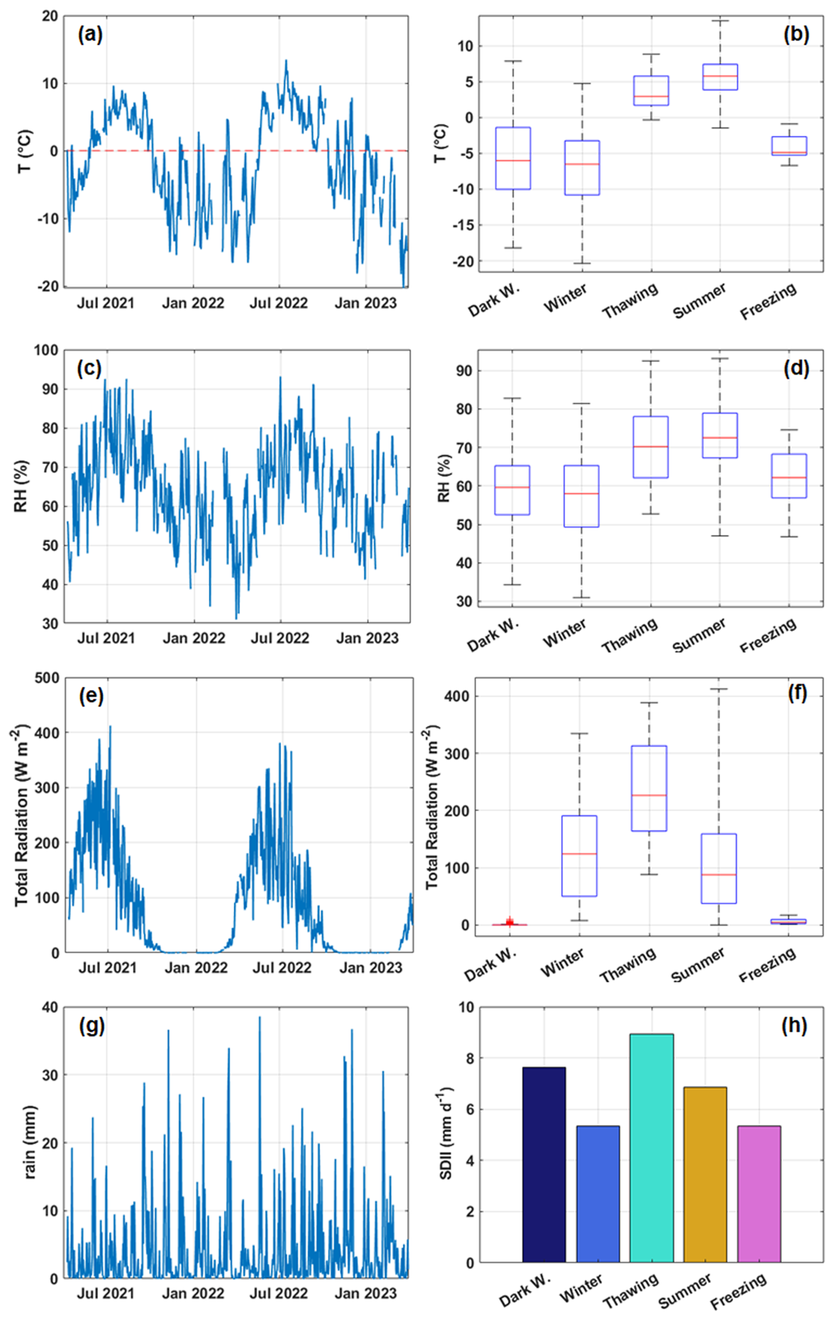
Figure B1 Time series and box plot with whiskers on daily and seasonal basis of (a, b) temperature (°C), (c, d) relative humidity (%), (e) total radiation (downward shortwave radiation) (W m⁻²), and (f) SDII (mm d⁻¹) at the CCT site. In the right panels, whiskers represent max and min values, and the box limits are the 25th and 75th percentiles. The red line represents the median value on a 30 min basis.

Appendix C: Micrometeorology at CCT for the measurement period

In the measurement period, sensible heat flux was on average negative (−6 W m⁻²) on a daily basis (Fig. C1a). The results show the presence of a long period with negative energy fluxes from the freezing to thawing season and a minimum around −77 W m⁻² until snow cover was present and during the melting snow phase, when the atmosphere was warmer than the surface. Sensible heat flux values had a positive magnitude (directed towards the atmosphere) for 32.7 % of cases, and for 67.3 % of events it was directed towards the snowpack. Upon thawing, a positive sensible heat flux became evident (see Fig. C1b), exhibiting median values of 4.2 W m⁻² (max 47 W m⁻²) in July, corresponding to the peak net solar radiation (253 W m⁻²) observed throughout the year. This behaviour had previously been observed in the Arctic (Kral et al., 2014; Donateo et al., 2023) where the snowpack acts as a sink of heat during the winter and spring months. In the freezing period, sensible heat fluxes were negative (median −6.04 W m⁻²), with daily averages down to −26 W m⁻², indicating energy moving towards the surface (Fig. C1b). Latent heat flux (Fig. C1c, d) had its minimum median value during the winter (light winter with a median of 1.19 W m⁻²), while its maximum median on a seasonal basis was reached during the summer (14.32 W m⁻²). Intermediate values were registered during the shoulder seasons, at 1.19 and 2.4 W m⁻² during thawing and freezing, respectively. In general, in this dataset no significant correlation between methane and latent heat fluxes has been observed (not shown here). Latent heat flux was positive for 76.2 % of the cases, while it was directed towards the soil in 23.7 % of cases. The median measured latent heat flux was 2.93 W m⁻² (8.48 W m⁻² on average) during the observation campaign. In Fig. C1e the time series of friction velocity shows a mean value of 0.19 m s⁻¹ for the whole measurement period. No specific differences can be noted in the friction velocity behaviour due to the changing snowpack characteristics or through the selected seasons. During winter, the friction velocity oscillated around a median value of 0.16 m s⁻¹. The thawing median value was slightly lower (about 0.13 m s⁻¹), while during summer the maximum values reached 0.15 m s⁻¹ (Fig. C1f). In particular, the frequency of stable and highly stable atmospheric conditions is 54 % and 13 %, respectively, of the total cases, while unstable and highly unstable conditions occur for 20 % and 12 %, respectively. Finally, neutral conditions were rare, showing a frequency below 1 %. Atmospheric stable conditions prevailed for the whole year, especially during the Arctic night (with a maximum stability parameter of 1.8). During dark and winter seasons, stable and very stable conditions were predominant (65 % and 16 %, respectively). Unstable atmospheric conditions arose only during the summer period with a median stability parameter of 0.47. In summer, there was a prevalence of unstable (33 %) and very unstable (20 %) conditions, with very stable cases below 10 %. The thawing season also exhibited a predominant stable situation (with 69 % of stable and very stable cases) with a median stability parameter of 0.22. The freezing season showed a stability frequency distribution like the previous shoulder season, with a higher prevalence of stable cases (60 %).

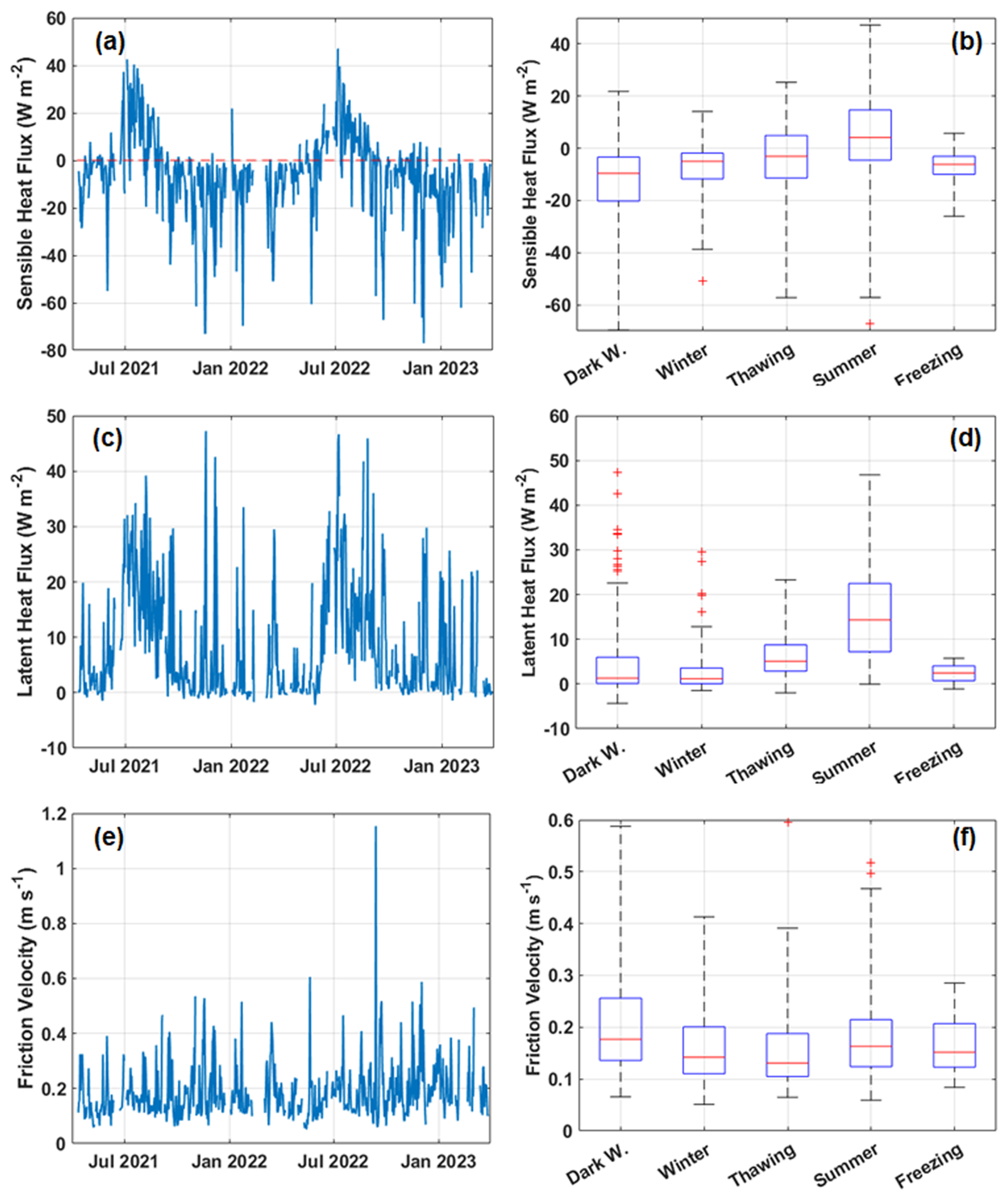
Figure C1 Time series on a daily basis (left) and whisker–box plots (right) of the principal micrometeorological variables measured during the campaign. (a, b) Sensible heat flux (W m⁻²), (c, d) latent heat flux (W m⁻²), and (e, f) friction velocity (m s⁻¹). In the right panels, whiskers represent max and min values, and the box limits are the 25th and 75th percentiles. The red line represents the median value on a 30 min basis.