Variability of CO₂ and CH₄ in a coastal peatland rewetted with brackish water from the Baltic Sea derived from autonomous high-resolution measurements

Rewetting peatlands is an important measure to reduce greenhouse gas (GHG) emissions from land use change. After rewetting, the areas can be highly heterogeneous in terms of GHG exchange and depend, for example, on water level, vegetation, temperature, previous use, and duration of rewetting. Here, we present a study of a coastal peatland that was rewetted by brackish water from the Baltic Sea and thus became part of the coastal shallow Baltic Sea water system through a permanent hydrological connection. Environmental heterogeneity and the brackish water column formation require improved quantification techniques to assess local sinks and sources of atmospheric GHGs. We conducted 9 weeks of autonomous and high-resolution, sensor-based bottom water measurements of marine physical and chemical variables at two locations in a permanently flooded peatland in summer 2021, the second year after rewetting. For the study, we used newly developed multi-sensor platforms (landers) customized for this operation. Results show considerable temporal fluctuations of CO₂ and CH₄, expressed as multi-day, diurnal, and event-based variability and spatial differences for variables dominantly influenced by biological processes. Episodic and diurnal drivers are identified and discussed based on Spearman correlation analysis. The multi-day variability resulted in a pronounced variability of measured GHG partial pressures during the deployment ranging between 295.0–8937.8 µatm (CO₂) and 22.8–2681.3 µatm (correspond to 42.7–3568.6 nmol L⁻¹; CH₄), respectively. In addition, the variability of the GHGs, temperature, and oxygen was characterized by pronounced diurnal cycles, resulting, for example, in a mean daily variability of 4066.9 µatm for CO₂ and 1769.6 µatm for CH₄. Depending on the location, the diurnal variability led to pronounced differences between the measurements during the day and night, so the CO₂ and CH₄ fluxes varied by a factor of 2.1–2.3 and 2.3–3.0, respectively, with higher fluxes occurring over daytime. The rewetted peatland was further impacted by fast system changes (events) such as storm, precipitation, and major water level changes, which impacted biogeochemical cycling and GHG partial pressures. The derived average GHG exchange amounted to 0.12±0.16 g m⁻² h⁻¹ (CO₂) and 0.51±0.56 mg m⁻² h⁻¹ (CH₄), respectively. These fluxes are high (CO₂) to low (CH₄) compared to studies from temperate peatlands rewetted with freshwater. Comparing these fluxes with the previous year (i.e., results from a reference study), the fluxes decreased by a factor of 1.9 and 2.6, respectively. This was potentially due to a progressive consumption of organic material, a suppression of CH₄ production, and aerobic and anaerobic oxidation of CH₄, indicating a positive evolution of the rewetted peatland into a site with moderate GHG emissions within the next years.

1 Introduction

Mitigating climate change requires a reduction in anthropogenic emissions of the greenhouse gases (GHGs) carbon dioxide (CO₂) and methane (CH₄) and the effective removal of CO₂ from the atmosphere (IPCC, 2023). In all climate scenarios with a realistic probability to reach the Paris Agreement, aiming to keep anthropogenic temperature increase “well below 2 °C” (IPCC, 2022a, 2023), land use, land use changes, and forestry (LUCLUF sector) play an important role. Still, a large part of the hard to abate residual emissions projected in these scenarios for the second half of this century come from the agricultural sector. Land use options with a large potential for climate mitigation include, for example, forestry, agriculture (pasture and cropland), wetlands, and bioenergy (Roe et al., 2019; IPCC, 2022b). In addition, in coastal areas, blue-carbon options such as restoration and expansion of mangroves, salt marshes, and seagrass meadows are suggested to have some potential for CO₂ removal (Duarte et al., 2013; Macreadie et al., 2019). The rewetting of formerly drained peatlands has been identified as one of the most promising approaches to lower CO₂ emission of used land, potentially even allowing turning (or re-establishing) some of these areas into CO₂ sinks (IPCC, 2014; Wilson et al., 2016). Peatlands cover vast areas in particular in northern Europe, northern Asia and western North America (based on data from the Global Peatland Database/Greifswald Mire Centre (2024)), and a large fraction of this area has been drained for agricultural use (UNEB, 2022).

Pristine peatlands and shallow coastal regions can act as sinks for CO₂ because they can store large amounts of carbon (C) when primary production exceeds mineralization and when organic matter (OM) is buried for long-term under anoxic conditions in peat soils (e.g., Mcleod et al., 2011; Harenda et al., 2018). One land use strategy that has emerged in recent years as an appropriate measure to reduce GHG emissions, particularly CO₂ emissions, is the rewetting of drained peatlands. In the temperate regions, many of these peatlands are in coastal areas where they are exposed to sea level rise and extreme weather events (UNEB, 2022). This leads to an increased connectivity at the terrestrial–marine interface (e.g., Jurasinski et al., 2018). As a result, coastal peatlands and their catchment areas are vulnerable to flooding and may become a part of shallow coastal waters due to passive or active inundation.

In general, GHG exchange in peatlands is sensitive to changes in the prevailing physical and biochemical conditions in the soil. For example, the water level, temperature, and vegetation mainly control the availability of oxygen (O₂) and thus the extent of oxic and anoxic zones (e.g., Parish, 2008; Kaat and Joosten, 2009). Pristine peatlands that are permanently or frequently saturated with water act as natural sinks for CO₂, as organic C is sequestered in anoxic zones, which results in the occurrence of peat accumulations. In turn, the anoxic conditions of waterlogged peat are very favorable for CH₄ production, making global peatlands a moderate source of methane of around 30 Tg CH₄ yr⁻¹ (Frolking et al., 2011). Freshwater and coastal ocean CH₄ sources have recently been identified as a major contributor to uncertainty for the global atmospheric methane budget (Rosentreter et al., 2024). When considering the total C budget, undisturbed peatlands are a weak C sink with around 100 Tg C yr⁻¹ (Frolking et al., 2011).

Drainage and lowering of the water column lead to infiltration of O₂ into the peat layers and aerobic decomposition of OM (Joosten and Clarke, 2002). As a result, drained peatlands become a strong source of CO₂, with reduced or negligible CH₄ emissions at water levels < 20 cm, since its production is strongly coupled with the water level (Kaat and Joosten, 2009). Drainage and prolonged decomposition also lead to a lowering of the general ground level, and especially drained coastal peatlands are therefore often below sea level.

Rewetting of degraded peatlands reduces CO₂ emissions by preventing aerobic decomposition of OM. The low solubility of O₂ and the slower transport across the overlying water body limits the availability of oxygen in the waterlogged peat soils for soil decomposition, which reduces aerobic mineralization and favors anoxic conditions, enhancing organic carbon burial (Parish, 2008; Kaat and Joosten, 2009). In the long-term, a re-establishment of the natural C-sink function could remove CO₂ from the atmosphere. The practice shows that rewetting with freshwater often leads to increased CH₄ emissions, while CO₂ emissions can remain high, at least for certain time after rewetting (Hahn-Schöfl et al., 2011; Hahn et al., 2015; Franz et al., 2016). These observations are primarily related to a wide range of preconditions and rewetting strategies and probably at least partly a transient phenomenon. Another strategy is the rewetting of coastal peatlands with brackish water. However, the effects of brackish water on GHG emissions are still unclear, although beneficial effects such as lower CH₄ emissions compared to rewetting with freshwater are likely due to the availability of sulfate (SO${}_{\mathrm{4}}^{\mathrm{2}-}$), a phenomenon better investigated for some coastal ecosystems, e.g., mangroves (Cotovicz et al., 2024). The availability of sulfate can promote the activity of sulfate-reducing bacteria (SRB). SRB can limit CH₄ production, as they outcompete methane-producing microorganisms (methanogens) for substrates (Segers and Kengen, 1998; Jørgensen, 2006; Segarra et al., 2013). Further, the availability of SO${}_{\mathrm{4}}^{\mathrm{2}-}$ favors anaerobic oxidation of methane (AOM), which could keep CH₄ emissions low (e.g., Boetius et al., 2000; Knittel and Boetius, 2009).

The spatial and temporal heterogeneity of environmental conditions is particularly noticeable in the coastal ecosystems of the Baltic Sea and is determined, for example, by the rapid cycling of elements (HELCOM, 2018; Kuliñski et al., 2022) and regular diurnal cyclicity (Honkanen et al., 2021). This becomes more pronounced when coastal peatlands have been rewetted with water from the Baltic Sea, thereby becoming part of the coastal water system of this marginal sea, as this results in very shallow subsystems that are rich in organic material and are in a transitional state. Those conditions are challenging for conventional sampling approaches, such as discrete water samplings (i.e., one-point recording), which cannot adequately resolve the temporal heterogeneity. As a result, systematic long-term data on GHGs with an appropriate resolution are very rare, and studies focus on open waters, estuaries, and discrete samplings. Consequently, coastal zones are not well-implemented in the global C budget due to difficulties in scaling processes (Saunois et al., 2020). Therefore, new techniques and interdisciplinary approaches are essential to address the blind spots and to establish a better monitoring of coastal regions. One possible approach for studying the highly dynamic coastal environment and evaluating the effectiveness of rewetting strategies is the use of autonomous in situ sensors, which can not only significantly increase the temporal resolution of data collection but also face problems such as limited battery power (Pönisch, 2023).

In this work, two newly developed, mostly identical lander systems were deployed, which are designed as autonomous platforms hosting a wide range of marine sensors. The landers were placed as fixed platforms on the sediment surface and were customized for this deployment with cabled power supply and uninterrupted high-resolution data acquisition. The systems can be considered modern, advanced technology for underwater monitoring applications, where sensor operation and sensor data acquisition are managed by a central data processing unit, which enables efficient processing of incoming data even during long-term missions.

We performed sensor measurements of the partial pressures of CO₂ and CH₄ and a suite of physicochemical variables, including water temperature, salinity, hydrostatic pressure, oxygen (O₂) saturation, turbidity, water velocity, and the concentrations of nitrate (NO${}_{\mathrm{3}}^{-}$), phosphate (PO${}_{\mathrm{4}}^{\mathrm{3}-}$), and chlorophyll a with high temporal resolution in the range of seconds and minutes in a recently flooded peatland over a period of around 9 weeks in the summer of 2021. The high-resolution measurements were combined with discrete sample analysis, and GHG emissions of CO₂ and CH₄ were derived.

The rewetting of the coastal peatland was achieved in November 2019, 2 years prior to this study, by the active dredging of a channel in the dike (Pönisch et al., 2023). This led to the formation of a permanent brackish water column and regular water exchange with the Kubitzer Bodden (Baltic Sea). Pönisch et al. (2023) showed that CO₂ fluxes were high in the first year of rewetting with brackish water, while CH₄ fluxes were low compared to freshwater rewetting. Their study however relied on weekly to biweekly discrete water sampling and could not resolve variability on shorter timescales.

The focus of this study is on exploring the timescales for the variability of GHG distribution and its drivers, as highly variable conditions are assumed. The 9-week time series is used to derive main cyclical as well as episodic variability in CO₂ and CH₄ concentrations and fluxes and to link it to physicochemical drivers. The impact of the temporal variability on the estimation of GHG emissions or with respect to discrete sampling strategies is assessed. By comparing GHG fluxes with a study conducted 1 year earlier (i.e., 2020, the first year after rewetting; Pönisch et al., 2023), the potential evolution towards further weakening of the CO₂ and CH₄ source strength is discussed.

2 Material and methods

2.1 The study site and lander locations

The measurements were conducted in the former Polder Drammendorf, a coastal peatland that was flooded with brackish water by an active removal of the protection measures in November 2019. The site is located on the southern Baltic Sea coast (Fig. 1a–b). The rewetting transformed the formerly drained and agriculturally used area into a permanently flooded brackish wetland with an estimated mean water column of ∼ 0.5 m (Fig. 1c). Flooding was accomplished by excavating an approximately 20 m wide section of the dike, creating a channel towards the Kubitzer Bodden, which in turn is connected via the Bodden chain to the Baltic Sea (Fig. 1). The peatland was flooded immediately since decades of peat degradation formed a land depression that is below the mean water level of the adjacent Kubitzer Bodden. The height of the water column of the flooded peatland depends on the water level of the micro-tidal Kubitzer Bodden and is described to be very dynamic (Pönisch et al., 2023). The exchange of water between the peatland and the Kubitzer Bodden takes place only via the channel; hence the hydrological connection acts as a transport route for dissolved compounds, such as nutrients or GHGs. An established hypsographic curve of the drained area allows calculation of water volume change from recorded sea level data; for details see Pönisch et al. (2023).

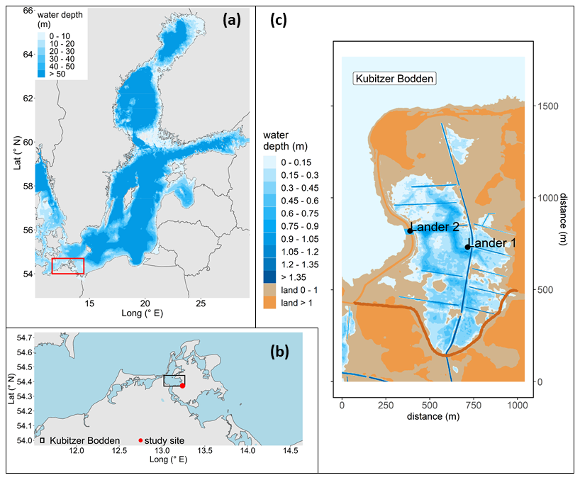
Figure 1 Location of the study site showing (a) the Baltic Sea with the study site located in the southern Baltic Sea, (b) the coastline of northeastern Germany with the study site located on the island of Rügen and its hydrological linkage to the Kubitzer Bodden, and (c) topography and water coverage of the study area at mean sea level as well as the locations of lander 1 (central area) and lander 2 (sea–peatland interface). The dark-brown line in the south shows the dike that was built before rewetting. Bathymetry refers to Seifert et al. (2001), and borders were retrieved from the National Oceanic and Atmospheric Administration (NOAA) and the National Centers for Environmental Information (NCEI).

The topsoil of the rewetted area is characterized by highly degraded peat up to 50–70 cm, with a well-preserved peat layer of ∼ 100 cm underneath (Brisch, 2015). The topsoil and vegetation were not removed prior to rewetting, and in the first months after rewetting, the former grassland and ditch vegetation (Elymus repens L. (Gould) and Phragmites australis (Cav.) Trin. ex Steud.) almost completely died out as a reaction of brackish inundation. As a result, the study site was initially characterized by high rates of carbon and nutrient cycling. The transition from dry to flooded conditions has been described in detail in Pönisch et al. (2023).

Two submersible landers equipped with sensors were used for autonomous multi-parameter investigations in the shallow water of the rewetted peatland through integrated high-resolution measurements. Lander 1 was deployed in the central part of the flooded peatland at a mean water depth of ∼ 0.6 m (Fig. 1c). Despite the frequent changes in the water level height (Fig. 2e), it can be assumed that the lateral water velocities are low due to the exposed location and that the effects of the processes associated with the peatland are pronounced. Lander 2 was installed in the middle of the excavated channel at a mean water depth of ∼ 0.9 m and thus at the interface between the Kubitzer Bodden and the peatland. This location allowed for the monitoring of the biogeochemical properties of the exchanging water masses. Due to the narrow channel and as indicated by a previous investigation (Pönisch et al., 2023), high, intermittent water flow velocities were assumed.

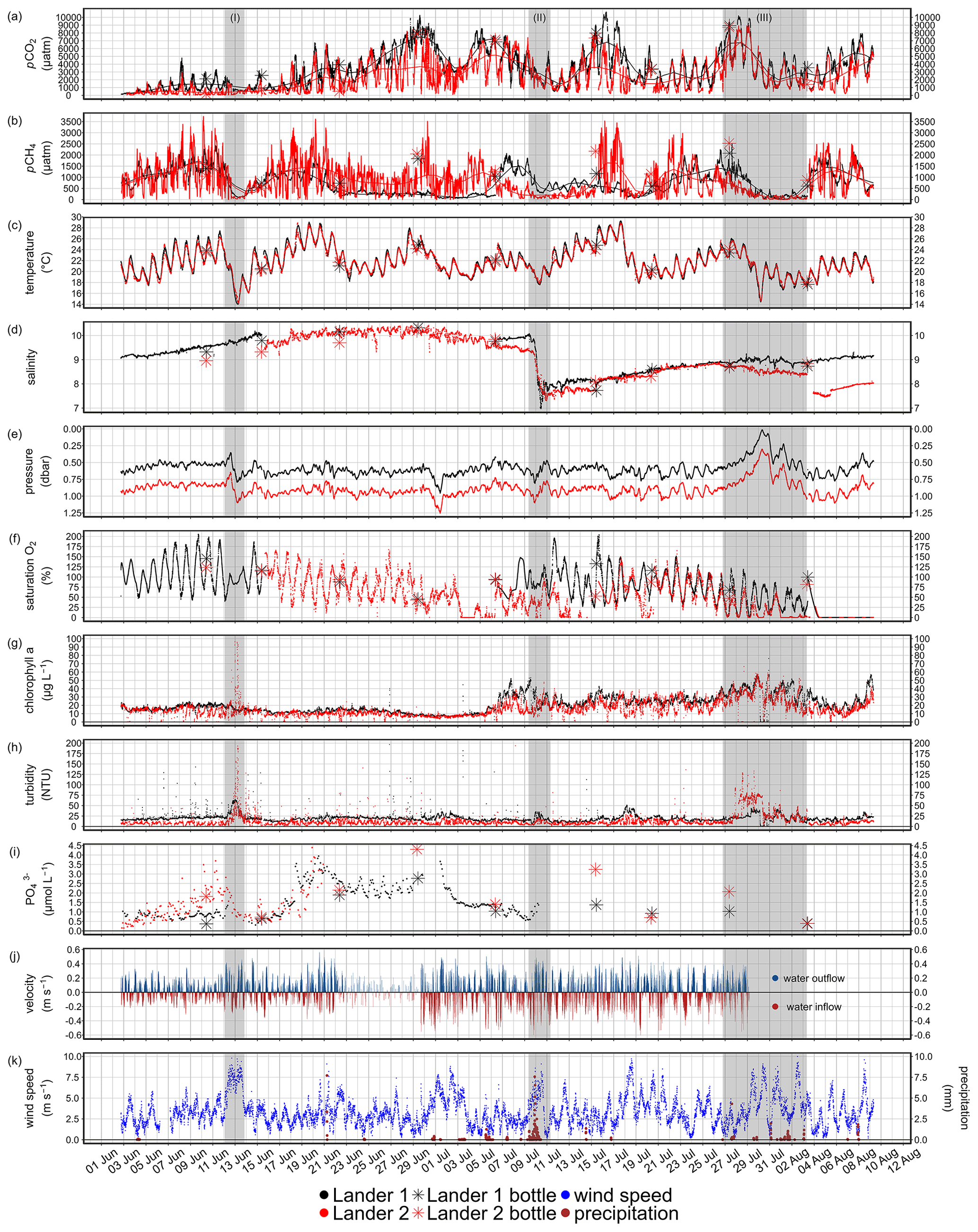
Figure 2 High-resolution time series from lander 1 (black) and lander 2 (red) with discrete bottle data (asterisks). The panels display post-processed data of (a) pCO₂ (µatm), (b) pCH₄ (µatm), (c) water temperature (°C), (d) salinity, (e) O₂ saturation (%), (f) hydrostatic pressure (depth; dbar), (g) chlorophyll a concentration (µg L⁻¹), (h) turbidity (NTU), (i) PO${}_{\mathrm{4}}^{\mathrm{3}-}$ concentration (µmol L⁻¹), and (j) wind speed (m s⁻¹) and precipitation (mm). The sensor signals of pCO₂ and pCH₄ were additionally smoothed, as represented by the black and red lines, respectively (description of smoothing is given in Appendix D). The gray rectangles highlight three periods of system changes (Sect. 3.3).

2.2 The landers

The two novel so-called landers are submersible platforms for advanced autonomous multi-parameter investigations in shallow water. The entirety of the carrier frame, the power supply, the technical units for sensor control, and the sensors are referred to as landers and were deployed as stationary measuring units at the sediment–water surface. Each lander system was equipped with state-of-the-art sensors that measured the partial pressures of CO₂ and CH₄ in the water, temperature, salinity, hydrostatic pressure, O₂, turbidity, and the concentrations of NO${}_{\mathrm{3}}^{-}$, PO${}_{\mathrm{4}}^{\mathrm{3}-}$, and chlorophyll a (Fig. A1). Sensor scheduling, time stamping, and data recording are centralized in the data processing unit (DPU) and allow customized deployments, for example long-term deployments or short-term deployments during extreme events such as storms. Despite a total weight of ∼ 250 kg, the modularity of the landers makes them ideal for areas that are highly dynamic and therefore cannot be studied with discrete samples. The landers were deployed and maintained using a small working boat, floats, and a lift system (Fig. A2). Both landers have already been described and deployed in a nearshore area of the Baltic Sea (Pönisch, 2023), but the system has been adapted in terms of power supply and communications (Fig. A1):

• The landers were powered by a professionally constructed 60 V land station near the observatories together with a 400 and 800 m cable. To compensate consumption peaks of the sensor, a buffer battery was included.

• The wired power cable for each lander was additionally used to establish a powerline communication and for SFTP and HTTP requests. This enabled on-air schedule adjustments, data access, and remote control.

• An IP socket was additionally used for power cycling (reset) of the systems.

The deployment took place between 2 June and 9 August 2021, and ∼ 500 000 data points were collected for each pCO₂ and pCH₄ sensor, respectively. The time of deployment was chosen based on the study of the annual cycle of GHG dynamics from the first year after rewetting and based on weekly to biweekly sampling (Pönisch et al., 2023), which indicated that the summer season is the most important and dynamic with respect to GHG fluxes.

2.3 Instrumentation

2.3.1 pCO₂ and pCH₄ measurements

Measurements of pCO₂ and pCH₄ with a logging interval of 10 s were carried out by submersible CONTROS HydroC^® CO₂ (HC–CO₂) and CONTROS HydroC^® CH₄ (HC–CH₄) sensors (-4H- JENA Engineering GmbH, Jena, Germany). Equilibration of gases in the seawater and the headspace in the sensor were achieved through a planar membrane, and the target molecules were detected by non-dispersive infrared spectrometry (NDIR; CO₂) and tunable diode laser absorption spectroscopy (TDLAS; CH₄), respectively (Fietzek et al., 2014). Further details on operation mode, sensor calibration, data post-processing, and quality assessment are described in Appendix C1–C3.

2.3.2 CTD–O₂ measurements

Conductivity, temperature, and pressure (CTD) and dissolved O₂ measurements were carried out with a SBE 37-SMP-ODO MicroCAT instrument (CTD–O₂; Sea-Bird Electronics Inc., Bellevue, WA, USA). The resolution of data acquisition was set to 5 min for lander 1 and 10 min for lander 2. A technical limitation led to the different recording interval. More information about sensor calibration, data post-processing, and data availability are provided in Appendix C4.

2.3.3 Turbidity and chlorophyll a concentration measurements

Turbidity and chlorophyll a concentrations were measured using SBE-FLNTUSB-ECO sensors (Sea-Bird Electronics Inc., Bellevue, WA, USA). Measurements were carried out with ∼ 1 Hz for 240 s followed by a 60 s sequence of bio-wiper/UV light treatment (information about the used UV light treatment is given in Appendix A2). The values were post-processed according to the calibration data provided by the manufacturer, and then the average values were calculated for each interval, which consisted of ∼ 240 individual measurements.

2.3.4 Nutrient (NO${}_{\mathrm{3}}^{-}$, PO${}_{\mathrm{4}}^{\mathrm{3}-}$) measurements

Nitrate concentrations were measured using SBE SUNA V2 instruments (Sea-Bird Electronics Inc., Bellevue, WA, USA) with a resolution of measurements of 10 min. The SUNA UV absorption spectra were processed according to Sakamoto et al. (2009) based on the calibration data provided by the manufacturer. Post-processing details are shown in Appendix C5.

Dissolved phosphate was measured using SBE HydroCycle-PO₄ sensors (Sea-Bird Electronics Inc., Bellevue, WA, USA), which were powered with an external battery and data logger. The phosphate sensors were not powered by the DPU due to technical restrictions. The resolution of the measurements was 60 min, with internal on-board calibration after six determinations. A five-point laboratory calibration was performed prior to deployment, and the field data were corrected with a linear regression model (R²= 0.9979 and 0.9987, respectively).

2.3.5 Water velocity measurements at lander 2

Lander 2 (position in the connecting channel) was additionally equipped with an upward-facing acoustic profiler (Aquadopp 1 MHz, Nortek AS, Norway) that was installed approximately 0.3 m above the sediment. The profiler recorded water velocities between 2 and 29 June 2021, in 50 mm cells at a sampling frequency of 1 Hz. The first bin was approximately 0.6 m above the bottom. In a second deployment a different setup of bursts of 600 s sampled with 4 Hz every 1200 s was programmed without changing the cell size. The second deployment was between 29 June and 29 July 2021. For the calculation of average velocities, the valid bins within the water column were first vertically averaged and then averaged over 120 s for the first deployment. For the second deployment the bursts of 600 s were averaged, yielding a vertically and time-averaged velocity every 10 min. To distinguish between in- and outflow into/from the peatland, the velocities were sorted in a way that all velocities with a direction between 30 and 200° were identified as an outflow, meaning that the water is flowing from the peatland to the Kubitzer Bodden (outflow; positive sign convention). Every other direction was defined as an inflow into the peatland.

2.4 Discrete field sampling and laboratory analysis of pH, total CO₂ (C_T), total alkalinity (A_T), CH₄, and nutrients (NO${}_{\mathrm{3}}^{-}$, PO${}_{\mathrm{4}}^{\mathrm{3}-}$)

To validate the sensor-based measurements, discrete field measurements were taken during the lander deployment at lander 1 (in the central peatland area) and at lander 2 (in the connecting channel). Undisturbed water was taken manually using a 5 L Niskin bottle. The bottle was deployed horizontally from a small working boat and its closure noted with an exact time stamp. Altogether nine sampling sessions were carried out in direct proximity to the landers (Table C1; bottle data for all discrete sampled variables can be found at https://doi.org/10.1594/PANGAEA.964758 (Pönisch et al., 2024)). Water from Niskin bottle sampling was analyzed using established laboratory methods as described below.

For laboratory analysis, subsamples from the Niskin bottle were taken by sample overflow for CH₄ (250 mL), pH (250 mL), and total CO₂ (C_T)/total alkalinity (A_T; 250 mL), poisoned with 500 µL (CH₄) and 200 µL (CO₂ system) of saturated HgCl₂ solution, respectively, and were stored at 4 °C in dark conditions. Nutrient subsamples (NO${}_{\mathrm{3}}^{-}$, PO${}_{\mathrm{4}}^{\mathrm{3}-}$; 200 mL) were filtered in the field with combusted glass-fiber filters (0.7 µm, GF/F, Whatman^®) and stored at −20 °C. Discrete samples for water temperature and salinity were measured in the field with a HACH HQ40D multimeter (HACH Lange GmbH, Düsseldorf, Germany) equipped with an electrode (CDC401).

The pH was analyzed by a spectrophotometric approach as described by Dickson et al. (2007) and Carter et al., (2013), using the pH-sensitive indicator dye m-cresol purple, and the values are reported on the total scale. C_T was measured with an automated infrared inorganic carbon analyzer (AIRICA; Marianda, Kiel, Germany). A_T was measured by potentiometric titration in the open-cell configuration described by Dickson et al. (2007). Dissolved CH₄ concentrations were determined using the gas chromatograph Agilent 7890B (Agilent Technologies, Santa Clara, USA) coupled with a flame ionization detector (FID) and based on the purge-and-trap technique (in-house designed periphery) as described in Sabbaghzadeh et al. (2021) and Pönisch et al. (2023). More details on the individual laboratory methods can be found in Appendix B. The analyses of NO${}_{\mathrm{3}}^{-}$ and PO${}_{\mathrm{4}}^{\mathrm{3}-}$ were carried out via standard photometric methods (Grasshoff et al., 2009), using a continuous segmented flow analyzer (Seal Analytical QuAAtro, SEAL Analytical GmbH, Norderstedt, Germany). Precisions and detection limits were ±4.6 % for NO${}_{\mathrm{3}}^{-}$ and ±4.0 % for PO${}_{\mathrm{4}}^{\mathrm{3}-}$ and 0.2 µmol L⁻¹ for NO${}_{\mathrm{3}}^{-}$ and 0.1 µmol L⁻¹ for PO${}_{\mathrm{4}}^{\mathrm{3}-}$, respectively.

2.5 Data handling and analysis

Data processing, analysis, and visualization were performed using R (R Core Team, 2022). The R packages that were used to calculate bottle data pCO₂ (based on bottle C_T and pH data), to convert pCH₄ (measured by HC–CH₄ sensors) to concentrations and CH₄ concentrations (derived from bottle data) to pCH₄ are described in Appendix D.

Spearman correlation coefficients (r_s) were calculated to provide an overview of the first-order linear relationship between the measured variables. To identify potential drivers, processes, and mechanisms of CO₂ and CH₄ variability, the presence or absence of (strong) correlations helps to identify and discuss potential causal relationships. A significance level of 0.001 was applied to identify non-correlating variables (empty boxes). In addition, a p-value adjustment was performed using the R package corrplot (Wei and Simko, 2021), as it is a multivariable correlation approach. To interpret the strength of the relationship between the variables, the convention of Cohen (1988) was used by introducing different effect sizes of correlations. An r_s≥0.5 and $r_{\mathrm{s}}\le -\mathrm{0.5}$ represents a large effect size and thus a strong correlation and is indicated by black stars. Accordingly, r_s≥0.3 and $r_{\mathrm{s}}\le -\mathrm{0.3}$ represents a medium effect size and correlation and is indicated by brown stars.

In order to show the diurnal cyclicity and the relationships between the variables affected by the diurnal cycles, the high-resolution measurement time series (lander 1 and lander 2) were divided into hourly bins, and a mean value was calculated for each hour of the day, resulting in a diurnal distribution pattern. Furthermore, to show the magnitude of diurnal variability of the variables, the mean diurnal variability was calculated. For this purpose, we divided the high-resolution data into 24 h intervals, each starting at midnight. Then, for each interval, the difference between the minimum and maximum was determined. Subsequent determination of the mean, minimum, and maximum yields an approximation of the magnitude of diurnal variability.

2.6 Air–sea exchange (ASE) calculation

The exchange (F) of CO₂ and CH₄ across the air–sea interface was calculated from the high-resolution measurements of pCO₂ and pCH₄ using the general boundary layer flux in Eq. (1) and the air–sea exchange parameterization of Wanninkhof (2014). The air–sea flux is determined by the difference in concentrations of the bulk liquid (c_w) in which the sensor measurements were carried out and the top of the liquid boundary layer adjacent to the atmosphere (c_a).

$$\begin{array}{}\text{(1)}& F=k\cdot (c_w-c_{\mathrm{a}})\end{array}$$

The gas transfer velocity (k) describes the efficiency of the transfer process and is parameterized as a function of the wind speed <U²>, an empirical relationship for the gas transport coefficient (0.251) and the Schmidt number (Sc; Eq. 2).

$$\begin{array}{}\text{(2)}& k=\mathrm{0.251}<U^{\mathrm{2}}>{\left(\mathit{Sc}/\mathrm{666}\right)}^{-\mathrm{0.5}}\end{array}$$

For the flux calculations, we assumed that the sensor-based GHG partial pressures were representative of surface water, since no permanent stratification occurred and the maximum water depth of the measurements was < 1.25 m. All involved variables (i.e., CO₂, CH₄, wind speed, temperature, salinity, atmospheric-equilibrium conditions) were averaged hourly to obtain more robust values and matching timestamps. Wind speeds at 15 m height were retrieved from a monitoring station in the vicinity (open data portal of the Deutscher Wetterdienst (DWD), Putbus station, distance ∼ 15 km, 54.36426° N, 13.47709° E, WMO-ID 10093). Since there were gaps in the measured salinity after post-processing (Fig. 2d), the values from both landers were combined by interleaving the values from lander 1 with those from lander 2. This procedure was justified because the locations of the two lander are physically connected by a strong water exchange, resulting in very similar salinity conditions, as shown in a previous study (Pönisch et al., 2023). The Schmidt number was approximated by a linear interpolation in salinity between the freshwater and seawater values (Wanninkhof, 2014). The Schmidt number depends on the gas, the temperature, and to a minor degree, the salinity of the water. The equilibrium concentrations (c_a) were calculated by using the values of atmospheric CO₂ and CH₄ mole fractions provided by the ICOS station Utö (Finnish Meteorological Institute, Helsinki, ICOS RI et al., 2022). The ASE model of Wanninkhof (2014) was developed for the open ocean waters and therefore may have reduced applicability for deriving GHG fluxes from an enclosed peatland. However, to the best of our knowledge no better suitable parameterization exists. Moreover, the same parameterization was used in Pönisch et al. (2023). The use of the same parameterization facilitated comparison of the results of our work with this previous study. We calculated the ASE for different sampling scenarios, to stress the effect of different methodologies and temporal sampling schemes:

1. ASE was derived from our entire high-resolution time series.

2. ASE was derived solely from the bottle data from our deployment.

3. ASE was derived from our high-resolution time series to represent the day–night bias. Daily averages for 00:00 UTC ± 1 h and 12:00 UTC ± 1 h were isolated (resulting in ∼ 200 data points for each calculation).

4. ASE was derived from the published data of Pönisch et al. (2023), where measurements were made in 2020, 1 year prior to our study. We chose the period corresponding to the period of this study (e.g., summer 2020).

5. ASE was derived from our high-resolution time series by isolating a daily average between 09:00 and 15:00 UTC. This time period represents the period of bottle data sampling in Pönisch et al. (2023), which is used for a direct comparison of the ASE evaluation described in number (4).

3 Results

3.1 Time series of the variables at lander 1 and lander 2

An overview of the time series data for the entire deployment is given in Fig. 2. For some of the variables, data are only available for parts of the time series, which can be easily derived from the figure.

Wind speeds were persistently weak to moderate with a mean of 3.4 m s⁻¹ (Fig. 2j) and ranged from 0.2 to 10 m s⁻¹, indicating that no strong storm occurred during the deployment. Furthermore, precipitation was low with a mean value of 0.08 mm h⁻¹ (corresponding to L m⁻² h⁻¹, data not shown).

The water column temperature at both landers showed considerable agreement in average and standard deviation (Table 1) as well as in the pronounced diurnal cycle (Fig. 2c). Within the period of simultaneously data coverage of both CTD–O₂ sensors, salinity also showed only small differences (Fig. 2d). In early July, salinity dropped by about 2–3, separating two periods of relatively stable salinity conditions. Furthermore, bottle data for salinity showed high agreement between both lander locations, supporting the pooling of salinity data from both landers for ASE calculation (Sect. 2.6). Taken together, the similar temperature and salinity indicate a distinctive water exchange among both landers and, hence, with the Kubitzer Bodden. This is supported by analysis of the hydrostatic pressure differences from both landers at 10 min intervals. For this, we calculated an average of the high-resolution data (Fig. 2e) every 10 min. The differences between both sites can be used as a proxy for water height compensation or the speed of water level height adjustment due to water exchange. The differences were only ±10 cm (minimum/maximum) or ±5 cm (0.98th percentile/0.02th percentile), respectively. We conclude that the adjustment of the water level is quasi-simultaneous between the locations of both landers due to the strong hydrological connection. Changes in water level (driven by changes in the connected Kubitzer Bodden) led to frequent alterations between inflow and outflow and drove high water velocities through the connection channel (position of lander 2), with the highest measured velocity of ±0.6 m s⁻¹ (Fig. E1). The frequent water level changes in alternating directions are also visible in the measured hydrostatic pressure at both landers, and hence frequent changes on the order of several centimeters occurred (i.e., ∼ 5–15 cm; Fig. 2e). These common inflows and outflows through the dike opening counteracted stagnant conditions due to water transport. As another important characteristic of the area of investigation, major changes in water level in relatively short periods of time were observed. For example, in late July, the water column height at both landers rose by 0.46 m within 11.5 h, followed by a period of rapid falling water level.

Oxygen exhibited large short-term fluctuations on a daily scale (Sect. 3.2), with saturation values ranging from ∼ 0 % to 180 %, indicating strong alternations between undersaturated and oversaturated conditions. Although occasionally low O₂ values were detected, measurements indicate a predominantly oxygenated water column, with slightly lower mean O₂ values at lander 2 (Fig. 2f, Table 1).

The pCO₂ varied considerably at both landers during the deployment displaying strong, multi-day, sinusoidal fluctuations (Fig. 2a) and short-term fluctuations < 1 d (Sect. 3.2, Table 1). Sustained lower average values occurred at the beginning of the deployment (early June) but then changed to on average higher values (> 1000 µatm) during most of the deployment at both locations. The general direction of change in the CO₂ signal on the multi-day scale was the same at both sites. While both landers exhibited comparable variability (i.e., standard deviation), lander 1 was characterized by a more than 1000 µatm higher mean pCO₂ (Table 1). At both landers, there was a negative correlation between pCO₂ and O₂ saturation with a strong effect size ($r_{\mathrm{s}}=-\mathrm{0.58}$, $r_{\mathrm{s}}=-\mathrm{0.56}$; Fig. 3). The comparison of the pCO₂ calculated from bottle C_T and pH data with the pCO₂ measured by the sensors showed both good agreements of only −2 % (a minus sign means lower values from the bottle data) and larger discrepancies of up to 45 % (Fig. C1). The median of the nine comparisons was 13 % for lander 1 and 12 % for lander 2.

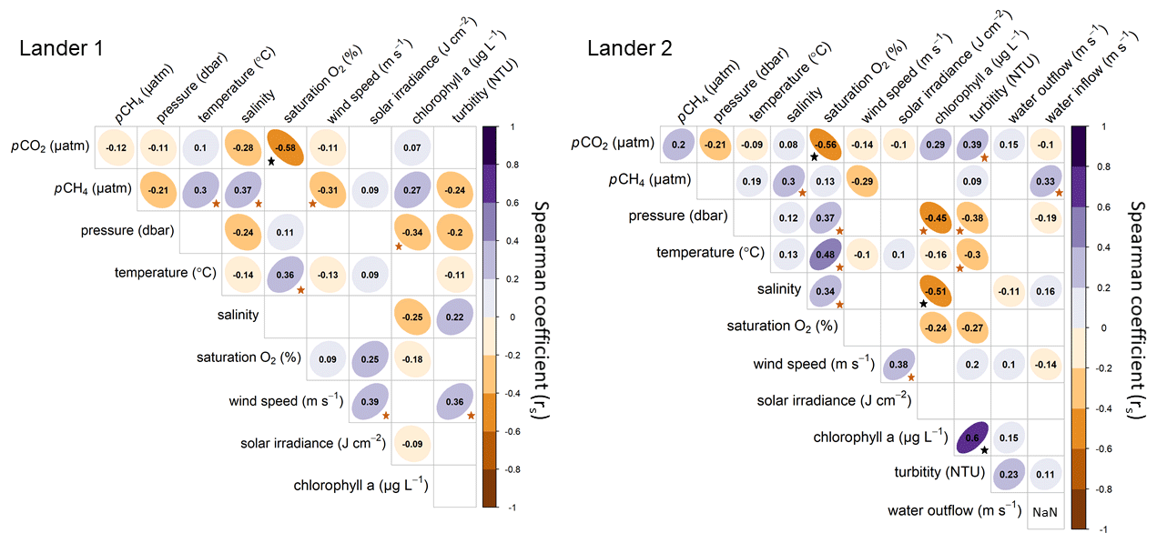
Figure 3 Spearman correlation coefficients (r_s) between the measured variables, wind speed, and solar irradiance of both landers. A correlation level of 0.001 was used to remove non-correlating relationships (empty fields). In addition, the Cohen convention (Cohen, 1988) was used to interpret the effect size. The black stars represent a large effect size and thus a strong correlation, while the brown stars represent a medium effect size. Wind speeds were retrieved from the station Putbus (WMO-ID 10093) and solar irradiance from Rostock-Warnemünde (WMO-ID 10170; both DWD).

The pCH₄ signals were characterized by strong and complex fluctuations manifested by multi-day variability during the deployment and by short-term fluctuations (< 1 d) that overlapped. The mean and SD of pCH₄ from lander 2 (dike opening) were slightly higher compared to lander 1 in the center of Polder Drammendorf (Fig. 2b, Table 1). Correlation analysis showed that pCH₄ at lander 1 had three dominant correlations, namely a positive correlation with temperature (r_s= 0.30) and salinity (r_s= 0.37) and a negative correlation with wind speed (r_s= −0.31; Fig. 3). At lander 2, the same correlations were visible but with lower effect sizes. In addition, pCH₄ at lander 2 had a positive correlation with a medium effect size with the velocity of the water outflow (r_s= 0.33). In comparison with the bottle data, where pCH₄ was calculated from cCH₄, the sensor pCH₄ data showed both good agreement with −21 % discrepancy but predominantly higher divergences reaching 595 % at maximum (Table C1). The median of the nine comparisons was 83 % for lander 1 and 77 % for lander 2, with the bottle data mostly higher than the sensor data.

Comparison of mean chlorophyll a concentrations and turbidity between the two landers showed slight differences, with higher values measured at lander 1 (Table 1). The time series of chlorophyll a revealed a more fluctuating pattern in the second half of the deployment (Fig. 2g). This observation was accompanied by a rapid decrease in salinity of about 3 within ∼ 1 d and followed by prolonged lower salinity until the end of the deployment. Accordingly, chlorophyll a on both landers showed a potentially significant negative correlation with salinity ($r_{\mathrm{s}}=-\mathrm{0.26}$, $r_{\mathrm{s}}=-\mathrm{0.27}$; Fig. 3). It also correlated negatively with hydrostatic pressure with a medium effect size at both landers ($r_{\mathrm{s}}=-\mathrm{0.34}$, $r_{\mathrm{s}}=-\mathrm{0.45}$). Turbidity indicated a possible positive relationship with the wind speed (r_s= 0.36), at least on lander 1. At lander 2, the turbidity showed a possible positive correlation with the water velocity (inflow and outflow; r_s= 0.23 and 0.11).

Sensor measurements of NO${}_{\mathrm{3}}^{-}$ are challenging in coastal areas because optical measurements are affected by several other absorbing species. Post-processing, including discrete colored dissolved organic matter (CDOM) measurements (data not shown), showed that spectra obtained from the SBE SUNA V2 instruments were dominated by CDOM interferences, which was not unexpected in the flooded peatland. At present, there are no advanced methods to distinguish between CDOM interference and NO${}_{\mathrm{3}}^{-}$ absorbance for application in the Baltic Sea or a peatland area. As a result, we had to conclude that the SUNA data are not suitable to derive NO${}_{\mathrm{3}}^{-}$ concentrations, in the present environment of very low NO${}_{\mathrm{3}}^{-}$ concentrations, since bottle data were predominantly below the detection limit (0.2 µmol L⁻¹; spectra data are available at https://doi.org/10.1594/PANGAEA.964839; Pönisch et al., 2024).

The phosphate measurements gave comparable mean values for both landers, although their periods of operation were quite different. Measurements at lander 1 ranged from 0.55 to 3.43 µmol L⁻¹ with a plateau of elevated values for ∼ 12 d in late June (Fig. 2i, Table 1). The sensor data were consistent with the bottle data.

Table 1 Summary of mean, standard deviation (SD), and minimum and maximum (as 0.98th and 0.02th percentiles) of available data from lander 1 and lander 2. Furthermore, the mean, minimum, and maximum of the calculated daily variability are shown (calculation is outlined in Sect. 3.2). CH₄ concentration (nmol L⁻¹) was calculated from pCH₄ (µatm). NO${}_{\mathrm{3}}^{-}$ concentrations could not be determined due to strong interferences with CDOM.

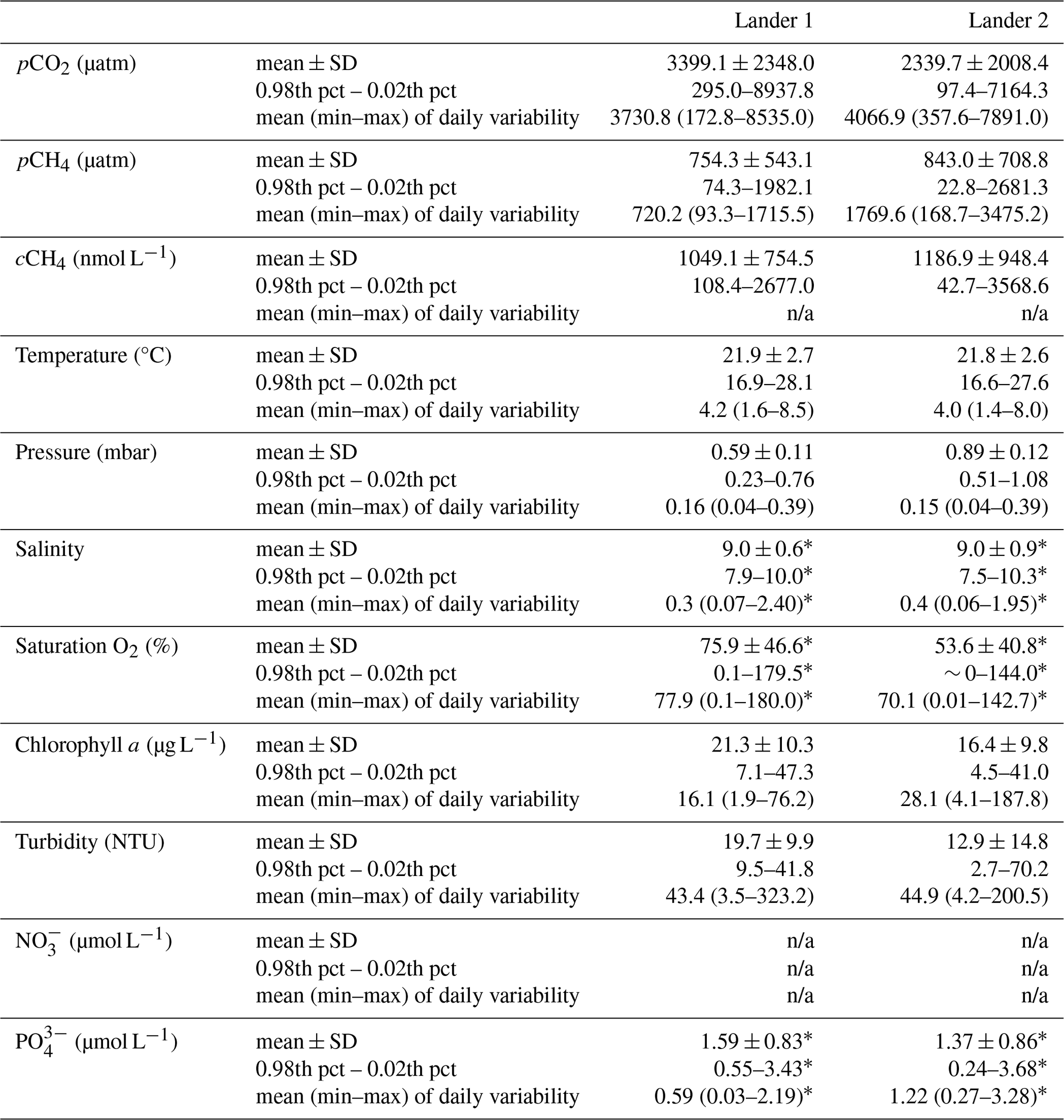
SD stands for standard deviation; pct stands for percentile; n/a stands for not applicable; data marked by an asterisk (^*) have major non-equivalent time coverage and are not comparable.

3.2 Short-term variability and diurnal cycles of the measured variables

The variables pCO₂, pCH₄, temperature, and oxygen showed pronounced short-term variability and diurnal cyclicity, expressed in regular sinusoidal fluctuations but sometimes superimposed by other fluctuations, especially for the GHG signals (Fig. 2). The diurnal cyclicity and the relationships between the variables affected by the diurnal cycles were made visible by calculating the distribution of hourly mean values (see Sect. 2.5). The distribution indicated that pCO₂ and pCH₄ showed an inverse character compared to temperature, O₂ saturation, and wind speed (Fig. 4). The highest mean pCO₂ values were observed in the early morning (05:00 UTC) and the lowest values in the late afternoon (17:00 UTC). The daily cycle of pCH₄ was less pronounced but also revealed higher values in the early morning (∼ 04:00 UTC) and lower values in the late afternoon (∼ 18:00 UTC). Furthermore, the wind speed was also characterized by a diurnal cycle, with higher speeds during the day and at midday, respectively. Since wind is used for the parameterization of the air–sea exchange, it has an influence on the determination of GHG emissions.

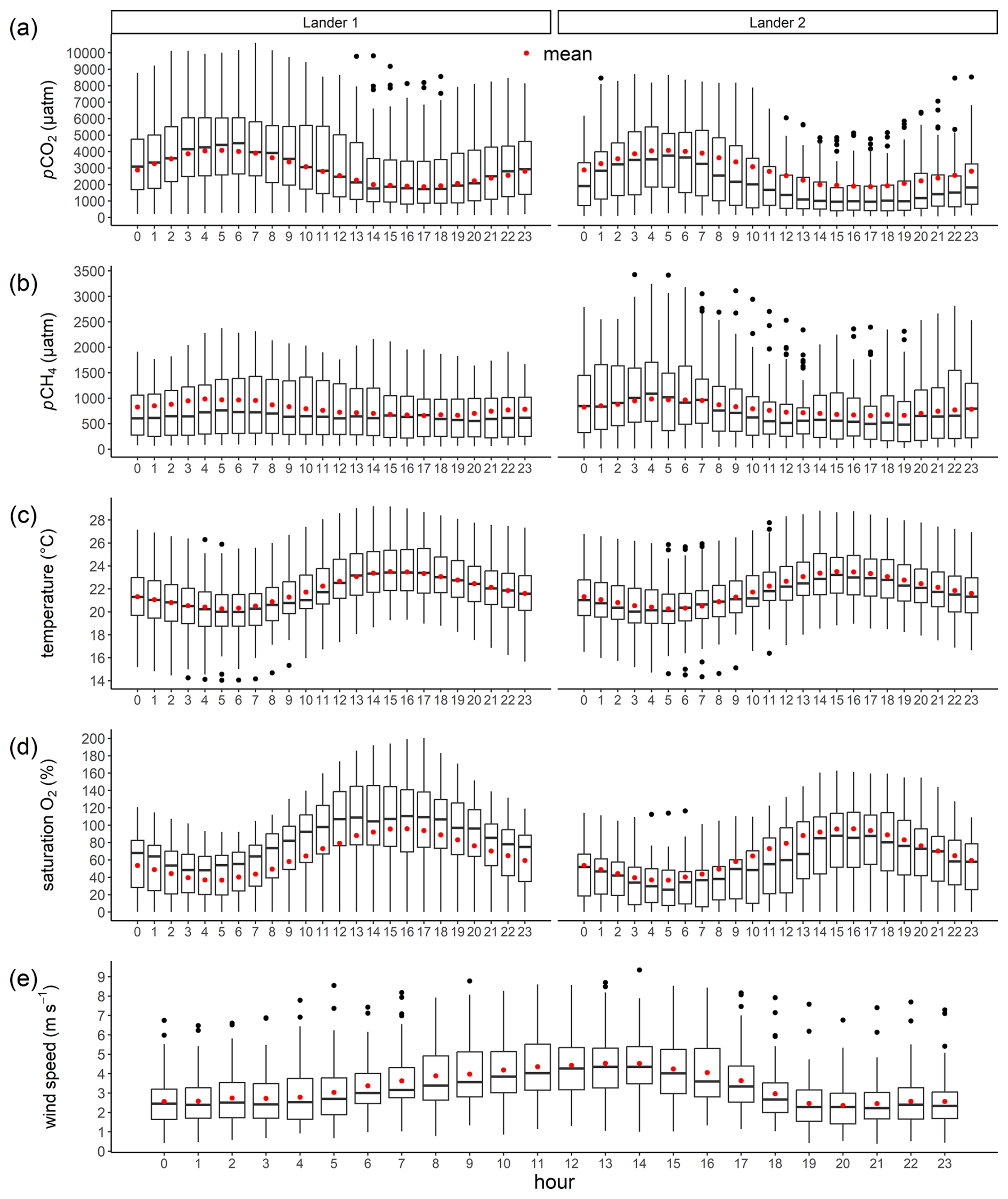
Figure 4 The daily cyclicity of the mean values of pCO₂, pCH₄, temperature, O₂, and wind speed derived from hourly binning. The box plots show the median and the 25th and 75th percentiles. The whiskers indicate the 5th and 95th percentiles, and the red points denote the mean values.

To show the magnitude of daily variability, the mean, minimum, and maximum of 24 h intervals were calculated (see Sect. 2.5) and summarized in Table 1. The mean daily range for pCO₂ of ∼ 4000 µatm is substantial. However, this diurnal range differed considerably during the deployment (Fig. 2a), with minimum and maximum daily variability ranging from ∼ 200 to ∼ 8500 µatm, with comparable patterns for both landers (Table 1). For pCH₄, the diurnal variability was also pronounced, but with larger differences between the two landers (Fig. 2b): the mean daily variability was ∼ 700 and ∼ 1800 µatm for lander 1 and lander 2, respectively. The observed minimum and maximum during the deployment ranged from ∼ 100 µatm to ∼ 3500 µatm (numbers for lander 2). On average, the temperature varied by ∼ 4°C and O₂ saturation by ∼ 70 %–75 % over the course of the day.

Analysis of the remaining variables (i.e., salinity, pressure, chlorophyll a, turbidity) revealed a low or non-diurnal behavior (Fig. E3). The relatively high mean daily variability for chlorophyll a and turbidity summarized in Table 1 is impacted by a large number of spikes and less by diurnal cyclicity.

3.3 Identification of three event-based system changes

Analysis of the meteorological, hydrographical, and biogeochemical parameters resulted in the identification of three events (Fig. 2, gray shaded periods). These observations are numbered as (I), (II), and (III) and are described in the following. They serve as exemplary time periods for detailed analysis of GHG drivers for the flooded peatland. Being more representative than the location at the connection between the Kubitzer Bodden and the rewetted peatland (i.e., position of lander 2), only data from lander 1 in the inner part of the formerly drained area were used. All three events, although different in nature, led to a disruption or at least dampening of the diurnal cycle of pCO₂ and pCH₄, as well as a reduction of the mean pCO₂ and pCH₄ values, for several days. Furthermore, pCO₂ and pCH₄ were strongly correlated during all three episodes (r_s= 0.73–0.86), and some of the correlation levels to individual drivers were far more pronounced for these shorter periods (Fig. E4).

3.3.1 Stormy event – (I)

Between 12–13 June 2021, a short-lived period with sustained high-wind speeds of up to 9–10 m s⁻¹ was identified. After an initial decline in water level, this resulted in a rise by ∼ 0.4 m with water from the Kubitzer Bodden entering the area of the rewetted peatland and led to an increase in water volume by 2.4 times compared to normal water level conditions (data not shown). Simultaneously, water temperature dropped by ∼ 13 K, while salinity remained unaffected. Turbidity increased and reached a pronounced peak of ∼ 60 NTU. The partial pressures of CO₂ and CH₄ decreased considerably, and the amplitude of the daily cyclicity of both GHGs and O₂ was substantially reduced for several days after the event. Correlation analysis revealed a number of correlations with strong and medium effect sizes (Fig. E4). For example, wind speed correlated with turbidity (r_s= 0.48). In addition, pCO₂ and pCH₄ correlated negatively with pressure (r_s= −0.66 and r_s= −0.87, respectively) and positively with temperature (r_s= 0.60 and 0.86, respectively).

3.3.2 Fast salinity decrease – (II)

The second event covers about 48 h in early July and was characterized by an accumulated precipitation of ∼ 76 L m⁻², corresponding to 1.6 L m⁻² h⁻¹. This resulted in a rapid (∼ 24 h) decrease in salinity by ∼ 2–3 and a concomitant outflow of water towards the Kubitzer Bodden, reinforced by a drop in sea level during the event. The freshwater impact also triggered a slight temperature decrease. On closer inspection, lander 1, which was shallower and enclosed, showed a greater decrease in salinity than lander 2. Chlorophyll a concentration and turbidity showed increased values, while GHGs decreased during this event. The pCH₄ showed a strong positive correlation with the salinity (r_s= 0.77).

3.3.3 Water outflow – (III)

In late July, we observed an outflow of water from the peatland towards the Kubitzer Bodden. The outflow caused a strong lowering in the water column, which drained large areas of the rewetted peatland and caused the pressure measurements of the CTD–O₂ sensor to reach ∼ 0 dbar. This drop in water level resulted in an estimated reduction in water volume by a factor of 5–6 compared to normal water level conditions. Nevertheless, the sensors were covered with water throughout the period, allowing uninterrupted data coverage. The outflow was slow and extended over several days with a subsequent rapid water inflow. Nighttime temperatures were coldest 1 d before the minimum water level was reached. Water level lowering triggered a decrease in pCO₂ and pCH₄ and a negative correlation with wind speed (r_s= −0.57 and r_s= −0.64, respectively), as well as a suppression of the amplitude of the diurnal cycles of both GHGs.

3.4 GHG fluxes derived from high-resolution data at lander 1 and lander 2

GHG fluxes for CO₂ and CH₄ were derived from the entire high-resolution sensor data and from different scenarios: from bottle data only, during daytime, during nighttime, and using data of a previous study to isolate GHG fluxes for a direct year-to-year comparison (Table 2).

Since the pCO₂ values were predominantly above atmospheric equilibrium during the deployment, a mean (±SD) CO₂ flux of 0.15 ± 0.18 g m⁻² h⁻¹ and 0.09 ± 0.13 g m⁻² h⁻¹ was determined for lander 1 and lander 2, respectively, with fluxes being persistently higher at lander 1 (Table 2). Nevertheless, a short period of CO₂ uptake occurred at both landers in the beginning of the deployment in early June (Fig. E2). The range of measured pCH₄ values indicated a permanent supersaturation compared to the atmospheric equilibrium. The resulting air–sea flux was 0.48 ± 0.51 mg m⁻² h⁻¹ and 0.54 ± 0.61 mg m⁻² h⁻¹ for lander 1 and lander 2, respectively (Table 2). The differences between GHG fluxes (CO₂ and CH₄) derived from daytime and nighttime are large, which is related to the diurnal cycles of the gas partial pressures and the wind speed (Fig. 4). Hence, atmospheric GHG fluxes are 2.1-fold (lander 2) and 2.3-fold (lander 1) higher for CO₂ and 2.3-fold (lander 2) and 3.0-fold (lander 1) higher for CH₄ during the day than at night (Table 2).

Table 2 Greenhouse gas fluxes were calculated for both lander positions as well as by using different data basis. The fluxes were calculated based on the sensor data¹ (bold), and for comparison, the GHG fluxes were additionally calculated using the bottle data². In addition, GHG fluxes were calculated based on the sensor data only for the daytime³ and nighttime³ to show the impact of diurnal effects. To obtain robust values, the sensor data for daytime and nighttime were each averaged by ±1 h. Moreover, we used the published data from Pönisch et al. (2023) to calculate the ASE for the corresponding period in 2020⁴, where investigations were conducted at the same study site during the first summer after rewetting (column “data from 2020”; data retrieved from the external source mentioned). In order to achieve the most comparable situation, we calculated the ASE based on the sensor data for the period between 09:00 and 15:00 UTC, since this is the period when the main sampling was performed in the mentioned reference⁵. The calculation procedure of (1)–(5) is described in Sect. 2.6.

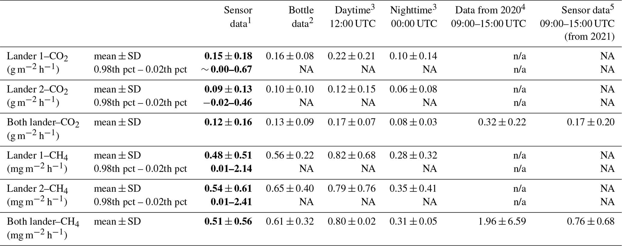
SD stands for standard deviation; pct stands for percentile; NA stands for not available; n/a stands for not applicable.

4 Discussion

For the deployment of two novel landers in the complex and heterogeneous environment of a rewetted peatland, it was important to integrate strategies to assess the quality of the sensor data. Therefore, we have conducted various measures and analyses to build confidence in the sensor data, which are discussed in detail in Appendix F1 together with the future implications for the deployment of the landers. Despite the fact that quality assessment turned out to be complex, we can show that the sensor data are suitable for interpretation based on two main analyses. First, the similarity of the main trends in the data series from both landers strongly suggests the appropriate sampling strategy for dynamic ecosystems. Second, with strong effort on discrete samplings and laboratory analysis, we observed both good agreement and discrepancies compared to the sensor data. Still, with all quality measures applied, we were able to achieve a robust post-processing which allows comprehensive biogeochemical interpretation, which we address in the following.

4.1 Biogeochemistry and driving parameters at the two observation sites

The deployment of two landers equipped with sensors for the high-resolution determination of marine variables pCO₂, pCH₄, temperature, salinity, hydrostatic pressure, O₂, turbidity, water velocity, c(PO${}_{\mathrm{4}}^{\mathrm{3}-}$), and chlorophyll a in a coastal peatland revealed large temporal and spatial variations of the measured variables. Temporal variability occurred on multi-day scales, diurnal scales, and through event-based changes, with spatial differences occurring for variables dominantly controlled by biological processes (e.g., GHGs). To our knowledge, there is no study that covers a comparable environmental setting with similar temporal data resolution. The range of variability was beyond time series for coastal areas which also exhibit diurnal cycles (e.g., Honkanen et al., 2021).

The time series of the physical parameters (i.e., temperature, salinity, water level) showed strongly fluctuating conditions on multi-day and daily scales, but the spatial differences between the two landers were very small. The latter reflects a strong spatial coupling between the two lander positions. The coupling is related, on the one hand, to the short distance between the two landers of ∼ 400 m and, on the other hand, to the pronounced water exchange with the adjacent Kubitzer Bodden driven by frequent water level changes. Together with wind-driven mixing of the shallow water column, this resulted in predominantly mixed water conditions, and thus O₂ consumption did not lead to long-term near-bottom anoxic conditions (Fig. 2f). This hydrologic coupling implies that the peatland became part of the coastal water region as a result of flooding (i.e., including transport of SO${}_{\mathrm{4}}^{\mathrm{2}-}$) and that biogeochemical patterns were influenced by processes occurring in the rewetted peatland as well as in the connected coastal shallow waters.

As a result of hydrological coupling, the time series of the GHGs at the two landers were also partially coupled, as evidenced by similar responses in the form of multi-day variability and event-based changes (Sect. 4.3). The multi-day variations, especially the decrease in pCO₂ and pCH₄, appear to be coupled to increased wind speeds after phases with low wind velocities, with a parallel decrease in temperature. Conversely, GHG concentrations increased again during periods of low winds, as also indicated by the slightly negative correlations of both GHGs with wind speed. With increasing wind, both ASE and water exchange with Kubitzer Bodden were enhanced. This facilitates a decrease of accumulated peatland GHG concentrations to atmospheric equilibrium – or coastal Baltic Sea (Bodden) background conditions. As a side effect, lower temperatures may occur due to deeper mixing in the adjacent Kubitzer Bodden. The multi-day accumulation is less visible for O₂ because of the faster re-equilibration with the atmosphere. Superimposed on the multi-day fluctuations are diurnal cycles, discussed in Sect. 4.2.

In addition to the patterns described above, spatial differences were found between the two landers for pCO₂, pCH₄, and O₂ and thus for variables that are affected by processes of biology, water transport, and air–sea exchange. The differences are mainly reflected in deviating values for mean and standard deviation (Table 1): while both landers exhibited comparable variability in pCO₂, lander 1 was characterized by a higher mean pCO₂. The higher values in the central peatland were associated with a high availability of OM for mineralization processes. The high availability could originate from various sources, e.g., from the flooded former vegetation and plant residuals that died after rewetting (Hahn-Schöfl et al., 2011), from the preserved or partially degraded peat layers, or from the OM supply from new primary production. The availability and decay of OM have already been identified as a major contributor to elevated CO₂ concentrations in a recent study, which covered the same study area in the first year after flooding (Pönisch et al., 2023). Since our investigations took place only 1 year later, comparable conditions can be expected.

A similar impact of the higher availability of OM in the central region was expected for pCH₄. The higher availability of readily degradable OM is a major driver for CH₄ formation (Heyer and Berger, 2000; Glatzel et al., 2008; Parish, 2008; Hahn-Schöfl et al., 2011) and should have resulted in higher CH₄ concentrations at lander 1. However, lander 2 showed slightly higher and more variable pCH₄ values, consistent with lower O₂ values. This was likely due to (i) a slightly deeper position compared to lander 1 (∼ 0.3 m deeper), which may lead to a faster expansion of CH₄-producing zones in the soil along with a stronger O₂ depletion during calm conditions, or to (ii) locally high water velocities and transport processes. The latter seems to be more important, as lander 2 was located in the narrow channel, where high water velocities occurred (Fig. E1). High water velocities can lead to local re-suspension, which in turn promotes pore water fluxes and can lead to the transport of soluble compounds into the water column (e.g., Massel, 2001; Beer et al., 2005), including CH₄ accumulated in the soil. The stronger control of the velocity is also visible since pCH₄ at lander 1 showed a more pronounced temperature control (Table 1). Temperature is another important driver of CH₄ concentrations, with higher CH₄ concentrations and fluxes occurring at higher temperatures (e.g., Bange et al., 1998; Heyer and Berger, 2000). The higher short-term fluctuations of the CH₄ signal (Fig. 2b) at the dike opening (lander 2), the higher mean concentrations, and the correlation with water movement suggest that the local position with high water transport rates and faster alteration of water supply from the Kubitzer Bodden and the drained peatland impacted the CH₄ signal at this location to some extent. Still, the relatively weak diurnal trend and major pattern during and following the discussed three major events (Sect. 4.3) are in unison.

4.2 Diurnal cycles and implication for discrete sampling

The solar irradiance causes diurnal cycles in the physics, chemistry, and biology of water bodies and has a particularly strong effect in shallow waters. As a result, diurnal cycles of pCO₂ and pCH₄ in shallow waters are coupled to a temperature-controlled cycle (i.e., solubility), air–sea gas exchange (i.e., wind parameterization), and biological processes influenced by eutrophic conditions and temperature (i.e., cycle of primary production and mineralization).

Binning the data set of the entire deployment by hours of daytime (Sect. 3.2) revealed that the highest GHG partial pressures (CO₂, CH₄) were observed in the morning and the lowest in the afternoon, with a more pronounced cyclicity for pCO₂ (Fig. 4). Temperature and O₂ saturation were also characterized by diurnal cycles, phase-shifted almost exactly by 12 h. In addition, a clear diurnal pattern is also visible for wind speed (Fig. 4e), enhanced during daytime and with a peak in the hours around noon, indicating a classical sea-breeze situation in summer.

Based on the diurnal water temperature cyclicity, one would expect lower GHG partial pressures to occur at lower temperatures and vice versa, due to the temperature-dependent solubility. Since this was not the case for pCO₂, the reduction in pCO₂ during daytime caused by primary production and increase during nighttime caused by mineralization clearly exceeded the temperature effect on solubility: during the day, the biologically controlled pCO₂ minimum exceeded the less influential temperature-controlled diurnal pCO₂ maximum. At night the opposite occurred, with mineralization being more important than cooling. The dominance of production (and mineralization) is supported by the strong negative correlation with O₂ (Fig. 3). The mean oxygen saturation of 75 % and 53 %, respectively, is in line with the high mean pCO₂ values, showing a general stronger contribution of mineralization than primary production. This relationship, representing a stronger biological control in comparison to the physical temperature-driven solubility effect, was recently described for pCO₂ for a shallow area on the Baltic coast near the island of Utö in August but with a much lower amplitude of 30 µatm (Honkanen et al., 2021).

The cyclicity of pCH₄ was lower and could be related to the higher O₂ availability and higher wind speeds during the day. In particular, the influence of wind speed – higher wind speeds favor the loss of CH₄ towards the atmosphere through air–sea exchange (Sect. 2.6) – likely contributed to the cyclicity in this shallow setting. In shallow waters, the ratio between water volume and water surface is low, and wind-driven reduction of concentrations towards atmospheric equilibrium is fast. Therefore, the higher wind speeds during the day likely contributed to the loss of CH₄ during daytime.

The diurnal cyclicity of GHGs, temperature, and O₂ in peatlands and/or coastal waters, along with possible additional spatial variability, must be considered when establishing sampling strategies. Discrete sampling campaigns, typically conducted during the day, appear questionable, as according to our data, they have a considerable bias. A suitable approach to capture these short-term temporal variations is the use of high-resolution, autonomous measurement techniques such as sensor-based or eddy covariance measurements. The potential influence of diurnal cycles in the flooded peatland during the winter months has not yet been investigated but is likely lower due to smaller daily changes in temperature. Also, as mentioned above, at least for our study site the summer had been identified as the season with strongest CH₄ and CO₂ dynamics based on discrete sampling in the year before (Pönisch et al., 2023).

4.3 Event-driven biogeochemistry in the semi-enclosed peatland

Three system changes occurred during the deployment, which, in addition to the multi-day and diurnal variability, represent another system-describing feature. Like diurnal cycles, these events can only be tracked by high-resolution measurements because changes occurred fast (on the order of hours and days). Although the flooded peatland is semi-enclosed with only a 20 m wide channel, water mass exchange occurs, and the Kubitzer Bodden acts as a start and endmember for external signals.

The first event (I) was characterized by elevated wind speeds leading to a short runoff, followed by a substantial inflow of water, a fast temperature drop of ∼ 13 K, a peak in turbidity, and lower GHG concentrations (Fig. 2). The inflow transported water with lower GHG concentrations from the Kubitzer Bodden and likely led to a dilution effect. In addition, strong cooling occurred during the event, with the strong temperature drop apparently caused by the incoming water from the Kubitzer Bodden, which got mixed by the strong winds and entrained colder deeper waters. The strong decrease in temperature likely led to reduced microbial activity, as this relationship has been described especially in coastal regions (e.g., Bange et al., 1998; Heyer and Berger, 2000). A reduced microbial activity is consistent with the drastically suppressed amplitude of the diurnal cycle of pCO₂ and pCH₄. During the event, turbidity increased at both lander positions, indicating increased re-suspension. Although re-suspension is known to potentially trigger the exchange of soluble compounds and GHGs between the sediment and the water column (e.g., Massel, 2001; Beer et al., 2005), this is not reflected in our data (i.e., comparably low pCO₂ and pCH₄ during the turbidity maximum). The partial pressures of the GHGs and the strength of the diurnal cycle recovered over the course of a few days and simultaneously returned to pre-event temperatures, consistent with the temperature and dilution that mainly caused the observations.

The second event (II) showed an impact of freshwater by precipitation and resulted in a fast drop of salinity within 1 d and a potential outflow of water due to a positive water balance. In addition, salinity remained low after this event and increased only slowly. Both GHG partial pressures showed a decline and a lower diurnal amplitude. It is assumed that a dilution effect occurred due to the precipitation, which was also described for event (I), as well as a transport of dissolved compounds towards Kubitzer Bodden due to the positive water balance. With strong precipitation, a transport of dissolved compounds, such as nutrients or organic material, from the terrestrial catchment into the peatland water is likely and could have influenced the GHG dynamics afterwards.

The third event (III) comprised a sustained outflow resulting in a water column of ∼ 0 m height at lander 1, followed by an inflow of water up to normal conditions. These very low water levels prevailed for around 24 h. As a consequence of this event, water temperature, pCO₂, pCH₄, and O₂ decreased with an additional decline in diurnal amplitude. With the outflow and lower water volume together with ongoing GHG emissions, this likely led to a decrease in GHG concentrations in the water. In addition, larger areas of the shallow peatland fell dry, so O₂ may have infiltrated into the soil. O₂ penetration and lower temperature could have led to lower CH₄ production after the water level rose, resulting in low CH₄ concentrations in the water column for several days after the event.

All three events show a strong correlation (in fact the strongest Spearman correlation coefficients between all parameters) between pCO₂ and pCH₄ (Fig. E4). Also, correlations with the physical drivers, in particular temperature, salinity, and wind speed, are far more pronounced than for the entire data set (Figs. 3, E4). The stronger correlation with temperature during these shorter episodes, as the parameter most directly related to the diurnal cyclicity, is dominant in particular for events (I) and (III). It is noteworthy that this correlation, though clearly inferred from the visualization of the diurnal cycle (Fig. 4), is less pronounced for the entire data series in the Spearman correlation analysis (Fig. 3), indicating that the episodic changes and long-term trends partially hide this dependence on longer timescales. In summary, during short-term episodes of strong hydrographical forcing, both trace gases are strongly controlled by these physical drivers, leading to a very strong correlation.

4.4 Derived GHG fluxes from the flooded peatland

Greenhouse gas fluxes for CO₂ and CH₄ for summer 2021, in the second year after rewetting, could be derived from the high-resolution sensor data, as measurements were made narrowly below the water surface (< 1.25 m), and a direct coupling of water at the lander with the surface water is assumed. Although the peatland showed a slight CO₂ uptake in early June (Fig. E2a), accompanied by stable but slightly decreasing chlorophyll a concentrations, the ASE was clearly dominated by a flux of CO₂ to the atmosphere. This amounted to 0.12 ± 0.16 g m⁻² h⁻¹ derived from both landers. Increasing fluxes through early July stabilized with a simultaneous strong increase in chlorophyll a concentration. Overall, CO₂ emissions in the peatland were controlled by the simultaneous occurrence of primary production and mineralization, with the latter predominating for an overall net CO₂ outgassing. The derived CH₄ fluxes of 0.51 ± 0.56 mg m⁻² h⁻¹ showed a stable development during the measurement period with a slight trend to lower fluxes in August (Fig. E2b), also strongly controlled by mineralization processes of OM. In the following, we discuss these fluxes in the context of other coastal studies, also addressing the main findings of an apparently low CH₄ emission under brackish inundation, a decrease in summerly CO₂ and CH₄ emissions in comparison to the first year after inundation, and a strong diurnal cyclicity.

4.4.1 CO₂ and CH₄ fluxes at the land–sea interface

We put our derived GHG fluxes into a broader context by comparing them with fluxes reported for different ecosystems along the land–sea interface, summarized in Table F1.

CO₂ fluxes from our study are around 1 order of magnitude higher than those reported from other restored peatland sites. For example, 9 years after flooding with freshwater, CO₂ emissions from a shallow lake formed on a formerly drained fen varied from 0.02 g m⁻² h⁻¹ (open water) to 0.09 g m⁻² h⁻¹ (emergent vegetation stands; numbers adapted from Franz et al. (2016)). In a recent review, Bianchi et al. (2021) derived a negative flux of −0.04 g m⁻² h⁻¹ as mean of 38 studies on restored peatland sites, supporting the interest of peatland restoration as a mean for climate mitigation.

Compared to land-based emissions (e.g., from drained unutilized land, cropland or forestry), the fluxes from our study area are a factor of 2 higher (Tiemeyer et al., 2020). Rivers and streams in the temperate latitudes of Europe, which are to a large extent anthropologically influenced, have GHG fluxes of approximately the same order of magnitude as our study area, ranging between −0.03 and 0.24 g m⁻² h⁻¹ (Mwanake et al., 2023). Open, shallow waters, which are directly connected to processes on land via runoff, and often influenced by human activities, are sometimes reported as sources of CO₂. A comparison with these areas shows that the fluxes from the shallow waters of the Baltic Sea or the North Sea are much smaller than those from the rewetted brackish peatland (Thomas and Schneider, 1999; Löffler et al., 2012).

The derived CH₄ fluxes of 0.51 ± 0.56 mg m⁻² h⁻¹ from our study are significantly lower than those reported for temperate fens rewetted with freshwater with comparable environmental settings (Hahn et al., 2015; Franz et al., 2016). For example, CH₄ emissions from the shallow lake mentioned above varied from 1.48 mg m⁻² h⁻¹ (emergent vegetation stands) to 6.05 mg m⁻² h⁻¹ (open water) even 9 years after rewetting (numbers adapted from Franz et al., 2016). In another study, where a dry fen was converted to a shallow lake with occasional brackish water impact, a CH₄ flux of 29.68 mg m⁻² h⁻¹ was reported in the first year after rewetting (Hahn et al., 2015).

The derived CH₄ fluxes of our study are in the same range as those from drained unutilized CH₄ emissions from land (Tiemeyer et al., 2020). CH₄ fluxes from the German section of the Danube River ranged between 1.3–12.8 mg m⁻² h⁻¹ (Lorke and Burgis, 2018), considerably higher than the fluxes derived in our study. A wide range of CH₄ emission rates have been reported from shallow coastal waters; e.g., very high CH₄ fluxes have been reported from the shallow waters of the Baltic Sea in summer, ranging from 39.9–104.2 mg m⁻² h⁻¹, while fluxes from 0.015–0.024 mg m⁻² h⁻¹ have been reported for continental shelves (Bange et al., 1994; Heyer and Berger, 2000).

The high CO₂ and low CH₄ fluxes from our study compared to other studies of rewetted peatland support the hypothesis of GHG fluxes that are still high but decreasing after a major perturbation (see next section) but with generally low CH₄ emissions compared to systems inundated with freshwater. While the theoretical background strongly supports the hypothesis of reduced CH₄ fluxes in the presence of sulfate, the empirical evidence for rewetted peatlands is still sparse. However, for mangroves, another coastal ecosystem group with climate mitigation potential, it has been recently shown that the offset of climate mitigation potential of mangroves was directly correlated with salinity, with the lowest offset (i.e., lowest methane fluxes in relation to carbon sequestration) in high-salinity regimes (Cotovicz et al., 2024). Based on the results of our study, the few studies on brackish water rewetting of peatlands, and studies on the blue-carbon potential of coastal ecosystems, the question of rewetting of peatlands with brackish or freshwater might play an important role for the climate mitigation potential and should be considered where both options are possible.

4.4.2 GHG flux development of the peatland in the second year after rewetting

Most of the studies mentioned above report annual GHG fluxes. Since our study only covers the summer months, comparability with these studies is limited, as annual CO₂ and CH₄ emissions are normally highest in the late summer months. To allow a more direct comparison of the development of the GHG emissions at our study site, we used the published data of Pönisch et al. (2023). These data covered the entire year 2020 from the same peatland area, 1 year prior to the study presented here. The system was described as nitrogen-limited, with availability of PO${}_{\mathrm{4}}^{\mathrm{3}-}$ in the summer, and this is in line with the conditions observed in our study, where discrete samplings for NO${}_{\mathrm{3}}^{-}$ were predominantly below the detection limit (data not shown), while PO${}_{\mathrm{4}}^{\mathrm{3}-}$ was available (Fig. 2). From the data of Pönisch et al. (2023), we isolated the same period during which the high-resolution measurements were made with the landers to assess the evolution of the ASE over 1 year (i.e., comparing summer 2020 and summer 2021). From Pönisch et al. (2023) we used ∼ 190 measurements for summer 2020, with ∼ 35 measurements from the peatland and the remaining from a transect in the vicinity of the later lander 1. We adjusted our high-resolution data to the conditions of their study by using a daily average value of data between 09:00 and 15:00 UTC (Table 2), as discrete sampling was conducted within this time window in the campaign of the year 2020 (Pönisch et al., 2023).

In addition to a high degree of comparability due to comparable boundary conditions, this approach also has limitations. The most important of these are a slightly different sampling height, which was ∼ 20 cm below the water surface in Pönisch et al. (2023) and ∼ 60–90 cm in our study; a different sampling approach; and possible inter-annual variations, which cannot be addressed with only 2 years of data. Therefore, the comparison only allows the indication of a trend that must be confirmed within further studies.

The comparison suggests that the CO₂ and CH₄ fluxes in the second summer after inundation were lower by a factor of 1.9 and 2.6, respectively, compared to the first (Table 2). A bias by the different sampling approaches appears negligible, as the fluxes calculated from the 9:00 to 15:00 UTC time interval of the high-resolution data and the fluxes just based on the bottle data (low resolution but directly comparable with the earlier study from a methodological point of view) are very similar (Table 2). Although, as mentioned above, interannual variability rather than a trend cannot be excluded in the second year after inundation, the reduction in CO₂ and CH₄ emissions is perfectly in line with the hypothesis of decreasing GHG fluxes in the years following the inundation. In general, the decay of vegetation from the former drained peatland and the decomposition of the organic-rich top soil foster strong mineralization of OM and fuel CO₂ and CH₄ production (Heyer and Berger, 2000; Hahn-Schöfl et al., 2011). Our findings are in line with the results of a recent study on the long-term development of a rewetted fen in northeastern Germany (Kalhori et al., 2024). The authors monitored the CO₂ and CH₄ fluxes over a period of 13 years and found a decreasing trend of CO₂ and CH₄ emissions and a switch from a CO₂ source to a CO₂ sink after more than a decade. With decreasing availability of degradable OM, stabilization of the microbial communities and potentially the establishment of new vegetation characteristics for brackish wetlands, a further reduction in GHG emission is thus expected.

4.4.3 The impact of diurnal GHG variability on GHG flux estimates

The studied peatland revealed a high temporal variability with respect to GHG partial pressures and other variables, characterized by multi-day and diurnal variations, with strong consequences for ASE estimates. To evaluate the impact, we calculated GHG fluxes from continuous time series when theoretically only (a) nighttime or (b) daytime was sampled to show the day–night bias and ASE only from (c) bottle data (Table 2). The latter was done because there was a high discrepancy between sensor data and discrete samples in some cases (Table C1).

Comparison with the ASE derived from entire high-resolution data showed higher fluxes from bottle data, highest fluxes during daytime, and lowest fluxes during nighttime (Table 2). The factors of CO₂ and CH₄ emissions between daytime and nighttime were 2.1–2.3 and 2.3–3.0, respectively. In our case, bias was not only caused by the diurnal fluctuation of the GHG concentration data, but also superimposed by the diurnal modulation of wind speed (Fig. 4). Consequently, studies on organic-rich flooded peatlands and shallow coastal areas, which are based only on bottle data and typically conducted during daytime, may result in biased GHG flux estimations for CO₂ and CH₄ due to a strong impact of diurnal cyclicity. This is in line with the observations of diurnal cyclicity reported from other ecosystems important in the context of climate mitigation (e.g., Belikov et al., 2019; Huang et al., 2019; Metya et al., 2021). It is therefore recommended to adjust the sampling and calculation interval of the biogeochemical parameters as well as relevant parameters for flux estimation (e.g., wind speed) to resolve these internal frequencies.

5 Conclusion

The measurement of key marine physicochemical variables in a shallow brackish water column of a rewetted coastal peatland using sensor-equipped landers was, to the best of our knowledge, demonstrated for the first time. With the deployment of the sensor-equipped landers, new challenges arose, such as the extensive technical infrastructure required or the difficult conditions of the water-covered peatland. The latter has affected the reliability of the state-of-the-art sensors and led to lower data quality. However, this circumstance is less significant when considering the given amplitudes of the fluctuations of the system. With improvements, e.g., new pump generations, sensor measurements can become more reliable in the future. Overall, the lander-based autonomous monitoring technique used in this study was successful in capturing GHG variability in a shallow water environment.

The results showed that the rewetted peatland was characterized by a generally high system variability. In particular, GHG partial pressures were dominated by long-term (multi-day) variability and diurnal cycles. The short-term variability was pronounced for pCO₂ and O₂, as variables that are predominantly biologically influenced, but the temperature and pCH₄ were affected by fast changes as well as diurnal cyclicity. Derived from these observations, pronounced differences between daytime and nighttime can be resolved. Hence, to achieve a comprehensive biogeochemical interpretation, and in particular for the derivation of GHG fluxes, this diurnal effect must be considered in shallow coastal waters and rewetted peatlands with a permanent water column.

The evaluation of GHG fluxes showed that the almost permanently oversaturated conditions for pCO₂ and pCH₄ mean that the peatland was a source of atmospheric GHGs. Comparing the fluxes to a study conducted in the same area 1 year prior to our study, emissions decreased by a factor of 1.9 and 2.6, respectively. Although limited data comparability and potential interannual variability have to be acknowledged, the continued decline in GHG emissions, especially in the relatively low CH₄ emissions, is in line with the hypothesis of a positive evolution of the peatland into a potential C sink (or small CO₂ source) with comparably low CH₄ emissions under brackish water influence.

The rewetting of formerly drained peatlands and the extension of shallow coastal ecosystems are currently discussed as potential measures for GHG emission reduction or even the creation of net negative emissions (CDR in blue-carbon schemes). Our study strongly suggests that the monitoring, reporting, and verification (MRV) schemes for these measures might require integrated assessment of carbon burial and GHG emissions, and the short-term variability and cyclicity might require new observational approaches to resolve the appropriate timescales. Moreover, time-integrated monitoring – as well as accounting – for several years after perturbation (i.e., rewetting) is required to correctly assess the potential and true impact of peatland restoration and other land-use-change options for climate mitigation.

Appendix A: The landers

A1 The lander concept

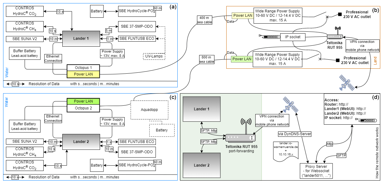
Figure A1 The detailed overview of the measuring system, including the landers (a, c), the power supply on land site (b), and the remote access configuration (d). (a, c) A dashed line represents equipment, which was used only for the actual lander. The captions at the arrows describe the resolution of measurements. Both landers were connected by a wired cable connection to ensure (b) power supply and powerline communication. The hardware for this approach was bundled in the in-house-developed “Octopus” device. The station on land enables remote power cycling and provides hardware for power supply and VPN connection. (d) A schematic flowchart of the used VPN infrastructure, which enables control and adjustments to lander data and sensor schedules.

A2 Maintenance and biofouling

During the deployment, measures were taken to ensure consistent data collection, as the study site is known to be challenging for sensor measurements, e.g., due to biofouling and re-suspension of particulate material. Hence, eight maintenance and visual inspections were conducted to monitor and remove effects of biofouling (Fig. A2). Furthermore, pump systems and optical measurement ways were cleaned. To suppress biofouling, we installed two UV light antifouling devices developed at IOW on the CTD–O₂ and SBE-FLNTUSB-ECO instruments of lander 1. The UV light antifouling solution uses UV LEDs with a wavelength of 275 nm and customizable optics. The UV lamps were switched on for 25 s every 10 min. The development is patent pending under DE 10 2019 101 420.4 and was funded by the Bundesamt für Seeschifffahrt und Hydrographie (BSH). The technology is licensed to Mariscope Meerestechnik e.K. (Kiel, Germany).

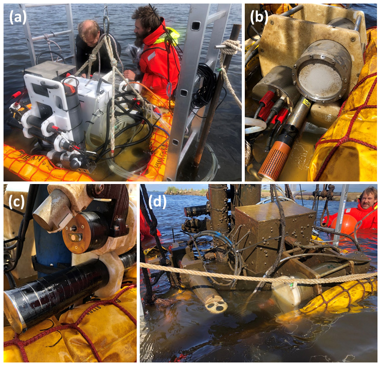
Figure A2 (a) Setting up the lander in the central area of the peatland using a lift construction, (b) image of the HC–CH₄ sensor during maintenance after ∼ 14 d of deployment, (c) setup and result of the UV antifouling device on the SBE-FLNTUSB-ECO instruments, and (d) the lander before recovery on the last day of the deployment.

Appendix B: Discrete sample analysis

B1 Analysis of pH

The pH was determined spectrophotometrically using the pH-sensitive indicator dye metacresol purple (mCP; 2 mmol L⁻¹; -4H- JENA Engineering GmbH, Jena, Germany), and the measurement principle and instrumental setup are described elsewhere (Dickson et al., 2007; Carter et al., 2013). The absorbance measurements were performed using the UV–VIS spectroscopy system Agilent 8453 (Agilent Technology, Waldbronn, Germany). The pH parameterization for brackish waters was calculated according Müller and Rehder (2018). A buffer solution with a salinity of 20, prepared according to Müller et al. (2018), and an external buffer solution with a salinity of 35 (University of California, San Diego (USA), Scripps Institution of Oceanography) were used for quality control.

B2 Total CO₂ (C_T) analysis

C_T was determined from discrete samples using the automated infrared inorganic carbon analyzer (AIRICA, MARIANDA, Kiel, Germany). The analysis was based on acidification of the sample (phosphoric acid, 10 %) followed by stripping of CO₂. The nitrogen carrier gas stream transported the released CO₂ to an infrared detector LI-7000 (LI-COR Environmental GmbH, Bad Homburg, Germany), via a Peltier cooler and a Nafion^® drying tube to remove water residues. Triplicate measurements and comparison to certified reference material (CRM; University of California, San Diego (USA), Scripps Institution of Oceanography; Dickson et al., 2003) allow the C_T to be calculated with a precision of ±5 µmol kg⁻¹.

B3 Total alkalinity (A_T) analysis

A_T was analyzed by open cell titration (glass electrode type LL Electrode plus 6.0262.100, Metrohm AG, Filderstadt, Germany) as described by Dickson et al. (2007) and involved a two-stage titration. After the first addition of hydrochloric acid to reach a pH of 4–3.5, A_T was determined during a stepwise titration to a pH of 3 while the pH was recorded potentiometrically. The calibration was carried out with the same CRM as used for C_T and allowed the same precision.

B4 CH₄ analysis

Dissolved CH₄ from bottle samples was measured using the GC Agilent 7890B gas chromatograph (Agilent Technologies, Santa Clara, USA) based on the purge-and-trap technique coupled with a flame ionization detector (FID), the details of which are described elsewhere (Sabbaghzadeh et al., 2021; Pönisch et al., 2023). A purified helium gas stream purges CH₄ and other volatile compounds out from the seawater sample and is subsequently dried by passing a Nafion^® tube (Perma Pure Nafion^®, Ansyco GmbH, Karlsruhe, Germany) and a SICAPENT^® tube (Merck KGaA, Darmstadt, Germany). CH₄ is accumulated by cryofocusing (−125 °C) on a trap filled with HayeSep D^® (CS Chromatographie Service GmbH, Langerwehe, Germany) using an ethanol / nitrogen cooling bath. After 10 min, the desorption occurs by heating the trap (water, 95 °C), and the separation of the target molecule from other compounds was achieved by two capillary columns and a Deans Switch (Pönisch, 2018). A CH₄ containing standard (9.9379 ± 0.0159 ppm) was measured daily before and after the sample measurement for quality control with a standard deviation of less than 1 %.

Appendix C: Sensors and data processing

C1 Sensor operation mode of HC–CO₂ sensors and data post-processing

The frequency of pCO₂ measurements was adjusted to 10 s, with 1 reading consisting of an average of 10 readings calculated by the sensor software. The HC–CO₂ sensors were operated with 1 W pumps (SBE-5M; Sea-Bird Electronics Inc., Bellevue, USA) and factory-calibrated for a measuring range of 200–6000 µatm before and after the deployment. The instruments regularly recorded zeroing values for 120 s by removing CO₂ from the gas stream every 12 h. The zeroing was followed by a flush period of 780 s and the signal readjusted to environment conditions. Zero and flush intervals were removed before biogeochemical analysis.

Post-processing of pCO₂, as described in Fietzek et al. (2014), was applied to the sensor data by including regular zeroing signals and a span drift correction using pre- and post-calibration polynomials. To correct the data for sensor response time (τ), the actual in situ τ was determined in advance for each flush period. The signal recovery after zeroing intervals was filtered based on standard deviation with respect to the predecessor and was set to < 5 µatm in a series of three values. The analysis of the pump power consumption during the deployment showed an occasional decrease reaching minimum values of ∼ 0.5 W (data not shown), resulting in a lower flow rate at the membrane and likely caused by a clogging of the filter basket and/or pump propeller due to sediment. As a result, the signal recovery to environmental conditions takes longer, and the selection criterion (standard deviation < 5 µatm in a series of three) was not achieved in every zeroing interval, and hence some in situ determination of the response times had to be discarded. The filtered data passing the selection criteria were used to fit an exponential function to the signal recovery and followed the descriptions of Fiedler et al. (2013) and Bittig et al. (2014). A mean τ of 329 and 380 s was obtained and used for data correction, while a rolling mean and median with a window width of 25 measurements before and after τ correction were applied to the response time correction to remove short-term noise. Short-term interruptions in the continuous data and artifacts from post-processing were removed.

The NDIR units were calibrated in the range between 200–6000 µatm, and the measured values exceeded this range occasionally and reached maxima of ∼ 10 000 µatm. Based on the calibration curve (not shown and provided by the manufacturer), the sensor followed a cubic signal-response, and extrapolation cannot be done with confidence. However, the lower range (< 2000 µatm) is described to be more cubic but is well described by the calibration. In a recent study, an NDIR unit was calibrated up to 25 000 µatm with only minor adjustments of the polynomial calibration curve (Canning et al., 2021). Hence, the accuracy of values exceeding 6000 µatm is slightly reduced, but we think that reporting these high pCO₂ values is of scientific importance. In support of this assumption, sensor data and bottle data were compared (Table C1), and this showed that the relative differences in the upper range compared to the lower range are not unremarkable.

C2 Sensor operation mode of HC–CH₄ sensors and data post-processing

The frequency of pCH₄ measurements was set to 10 s, with 1 reading consisting of an average of 10 readings calculated by the sensor software. The HC–CH₄ sensors were calibrated before and after deployment at 10 °C water temperature for a range of 1–40 000 µatm by the manufacturer, to prove the linearity and stability of the TDLAS unit throughout the deployment. Equipped with external 7.5 W pumps (SBE-5T; Sea-Bird Electronics Inc, Bellevue, USA), a response time of 2400 s was determined for both sensors. The analysis of the pump power consumption during the deployment showed an occasionally decrease reaching minimum values of ∼ 0.5 W (data not shown), resulting in a lower flow rate at the membrane and likely caused by a clogging of the filter basket and/or pump propeller due to sediment. Based on laboratory tests, pump consumption (W) can be converted to a water flow rate (L min⁻¹) and was simulated in the experiment with a SBE-5T pump between ∼ 5 W (maximal pump capacity) and ∼ 3 W (restricted pump capacity) due to artificial clogging of the filter basket. The decrease in water flow rate from ∼ 8 to ∼ 3 L min⁻¹ follows a linear slope (R²= 0.83), and the lower limit of the water flow rate is equivalent to a SBE-5M under maximal pump capacity. Based on this observation and to correct the in situ pCH₄ values, the response times for the HC–CH₄ were determined using a SBE-5T and SBE-5M pump, respectively, resulting in an increase of the response time by a factor of 1.7. Hence, we chose to linear interpolate the response time between the two limits (limits between maximum pump power of ∼ 6 and 3 W) and extrapolate when pump power was below the threshold of 3 W (Nadja Kinski, -4H- JENA Engineering GmbH, personal communication, 2022). Since biofouling can be neglected (regular maintenance and cleaning), the response time was not additionally affected. The interpolated / extrapolated response time ranged between 2400 and 4800 s and was used to correct the signal delay for each recorded pCH₄ value (same procedure like for HC–CO₂ sensor see above; described by Fiedler et al. (2013) and Bittig et al. (2014)). A rolling mean with a window width of 180 before and a rolling median with a window width of 50 measurements after the calculation of the in situ pCH₄ value were applied to remove short-term noise. Measurement interruptions and artifacts from post-processing lasting longer than 180 measurements were removed from the continuous data.

C3 Quality assessment of sensor GHG measurements

The application of the post-processing procedures described above (i.e., zeroing, span drift, and τ correction) led to an improvement of the sensor data. However, the study site is in particular characterized by conditions that are challenging for marine instrumentation, and no sophisticated hardware adjustment (i.e., pump operated reliable in flat water) or post-processing is available for these environmental conditions. This resulted in higher uncertainties in absolute pCO₂ and pCH₄ values. But, since ∼ 500 000 measurements are included for each compound, the time series is statistically robust. Nevertheless, some uncertainties will be mentioned in the following.

The pCO₂ values reached > 10 000 µatm and therefore exceeded the calibration range, resulting in greater uncertainties in the upper values.

The determination of in situ τ for pCO₂ was challenging during periods of low pump activity (i.e., ∼ 0.5 W power consumption), resulting in a higher spread for each actual τ determination and hence a slightly lower post-processing quality.

The above-mentioned issue resulted in the lack of a sufficient amount of calculated in situ τ during periods of lower pumping activity. Therefore, only an average τ could be calculated (i.e., 329 and 380 s).

The HC–CH₄ sensors occasionally showed gaps in the continuous data and rapid dynamics in the signal, which posed challenges for the post-processing techniques used. Consequently, a relatively wide window width for signal smoothing had to be applied (> 180 points); otherwise this would have resulted in many artifacts and values < 0 µatm. In turn, this signal smoothing resulted in a loss of micro-dynamics in the sensor signal, which can be quite pronounced compared to a narrower window widget. This is shown exemplarily in Fig. C1.

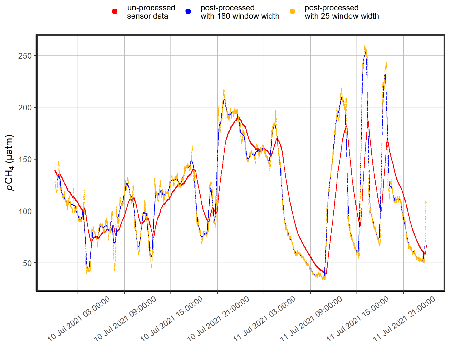
Figure C1 The effects of the different post-processing methods on the sensor data (red). Strong smoothing (blue) resulted in a lower level of signal detail compared to weak smoothing (gold), but the impact of different window widths is predominantly low.

Table C1 Direct comparison of the GHG partial pressures derived from sensor data with bottle data. Sensor values were obtained by calculating an average of a 10 min interval of the continuous data before discrete sampling. Values in bold show results for pCO₂ above the calibration range.

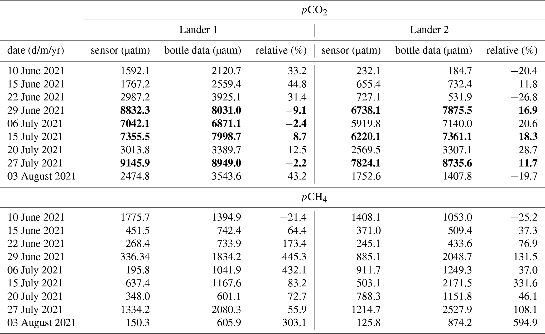
C4 Data post-processing of CTD–O₂ sensors

Pre-deployment calibration of temperature and salinity and post-calibration of the O₂ were carried out in the accredited calibration laboratory of the IOW. Accordingly, O₂ was calibrated against a reference optode at zero O₂ concentration and equilibrated O₂ concentration in a water bath, and this two-point calibration was used for a linear adjustment of the manufacturer calibration. The assessment and correction of the oxygen optode drift during the deployment time (∼ 9 weeks) were addressed by in-air oxygen optode measurements before and after the sensor deployment. A slope correction between measured in-air samples and the calculated atmospheric partial pressure was carried out each for pre- and post-deployment (Bittig and Körtzinger, 2015). The average of each slope correction was calculated; hence, a coefficient for correction of 1.056 and 1.033 for CTD–O₂ 20514 and 20515, respectively, was used. In occasional periods of the time series, O₂ and conductivity had to be removed from the data because the time series showed a non-comprehensible steep decrease in values and a discrepancy with discrete samples. This was likely related to the ingress of air bubbles into the measuring circuit. Although measures were taken to avoid these air locks during maintenance, the low pump capacity of the CTD–O₂ was unable to maintain a continuous, undisturbed air-free circuit. Temperature and pressure were unaffected due to their exposed position in the circuit.

C5 Data post-processing of SUNA V2 sensors (NO${}_{\mathrm{3}}^{-}$)

In the post-processing, in situ temperature-corrected salinity absorbance (bromide absorption) was subtracted from the total measured absorbance. The remaining temperature-corrected salinity-subtracted absorbance in the wavelength range 217–240 nm was used in a regression analysis with NO${}_{\mathrm{3}}^{-}$ absorbance and a linear baseline as components. In addition, the technical drift of light source intensity during the deployment was compensated by measuring the UV absorption spectra of Milli-Q water before and after the deployment. The post-processing revealed that the sensor spectra were dominated by CDOM interferences. Therefore, it was assumed that the SUNA data are not suitable for deriving NO${}_{\mathrm{3}}^{-}$ concentrations, in the present environment of very low NO${}_{\mathrm{3}}^{-}$ concentrations.

Appendix D: Data handling and calculations

The data processing, analysis, and visualization were carried out in R (R Core Team, 2022) by using the packages tidyverse (Wickham et al., 2019), patchwork (Pedersen, 2020), and DBI (Wickham and Müller, 2021). The data smoothing shown in Figs. 2 and E2 was performed with geom_smooth() using the method gam and values of k= 30 and 5, respectively.

Bottle data of C_T and pH were used to calculate pCO₂ (e.g., Fig. 2) by using the R package seacarb (Gattuso et al., 2019) with K₁ and K₂ from Millero (2010), K_s from Dickson (1990), and K_f from Dickson and Riley (1979).

CH₄ concentrations were calculated from sensor-based pCH₄ measurements by calculating a mean value for pCH₄, salinity, and temperature for 1 h periods. Since salinity is not consistently available at both landers, a combined salinity time series was created by filling the values from lander 1 with those from lander 2. This appears to be justified because the two landers are connected by a strong water exchange, resulting in very similar conditions in physical variables, as shown in our study as well as in a previous study (Pönisch et al., 2023). The conversion between pCH₄ and cCH₄ was performed according to Wiesenburg and Guinasso (1979).

Appendix E: Results

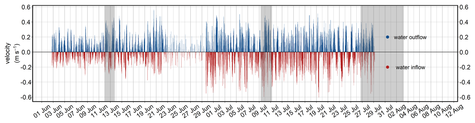
Figure E1 High-resolution time series of the water velocity (m s⁻¹) measured at lander 2. Water outflow means that water flows from the peatland toward the Kubitzer Bodden driven by changes in the water level and vice versa.

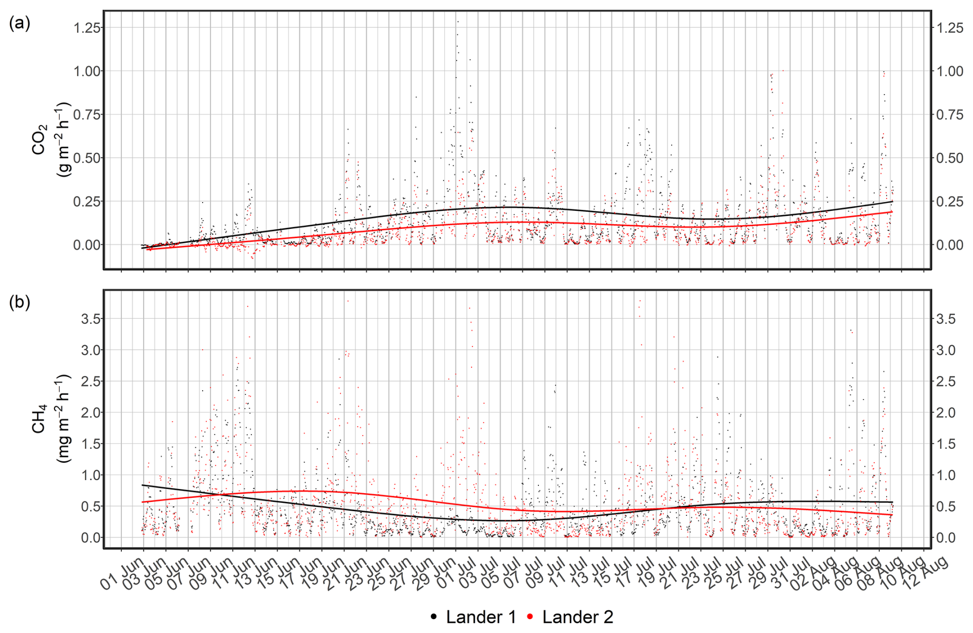
Figure E2 Calculated GHG fluxes using the Wanninkhof (2014) wind speed parameterization approach for CO₂ and CH₄ at both landers. A smoothing was used to highlight the trend and differences between the landers (description of smoothing is given in Appendix D).

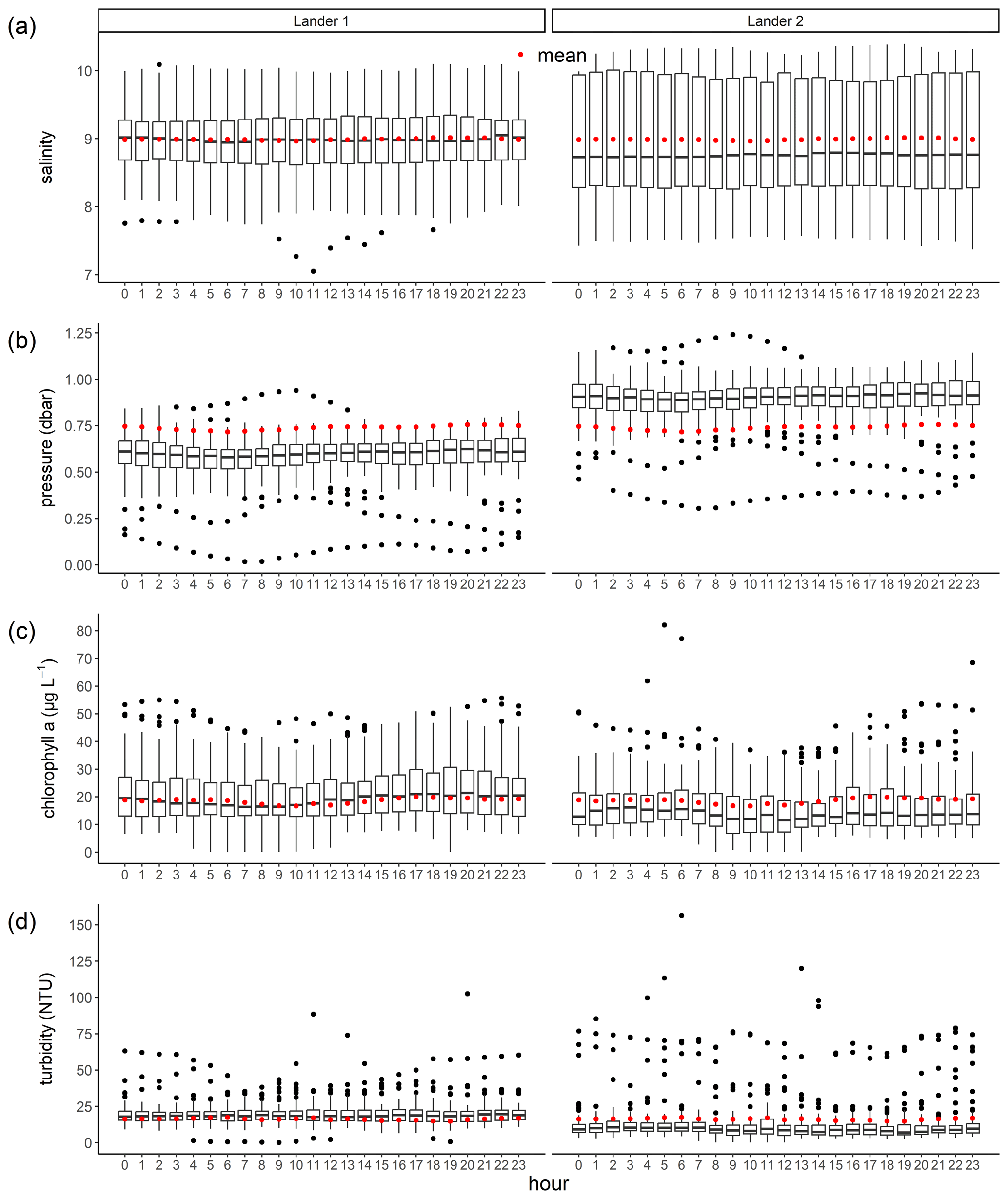
Figure E3 The daily cyclicity of the mean values of salinity, pressure, chlorophyll a, and turbidity derived from hourly binning. The box plots show the median and the 25th and 75th percentiles. The whiskers indicate the 5th and 95th percentiles, and the red points denote the mean values.

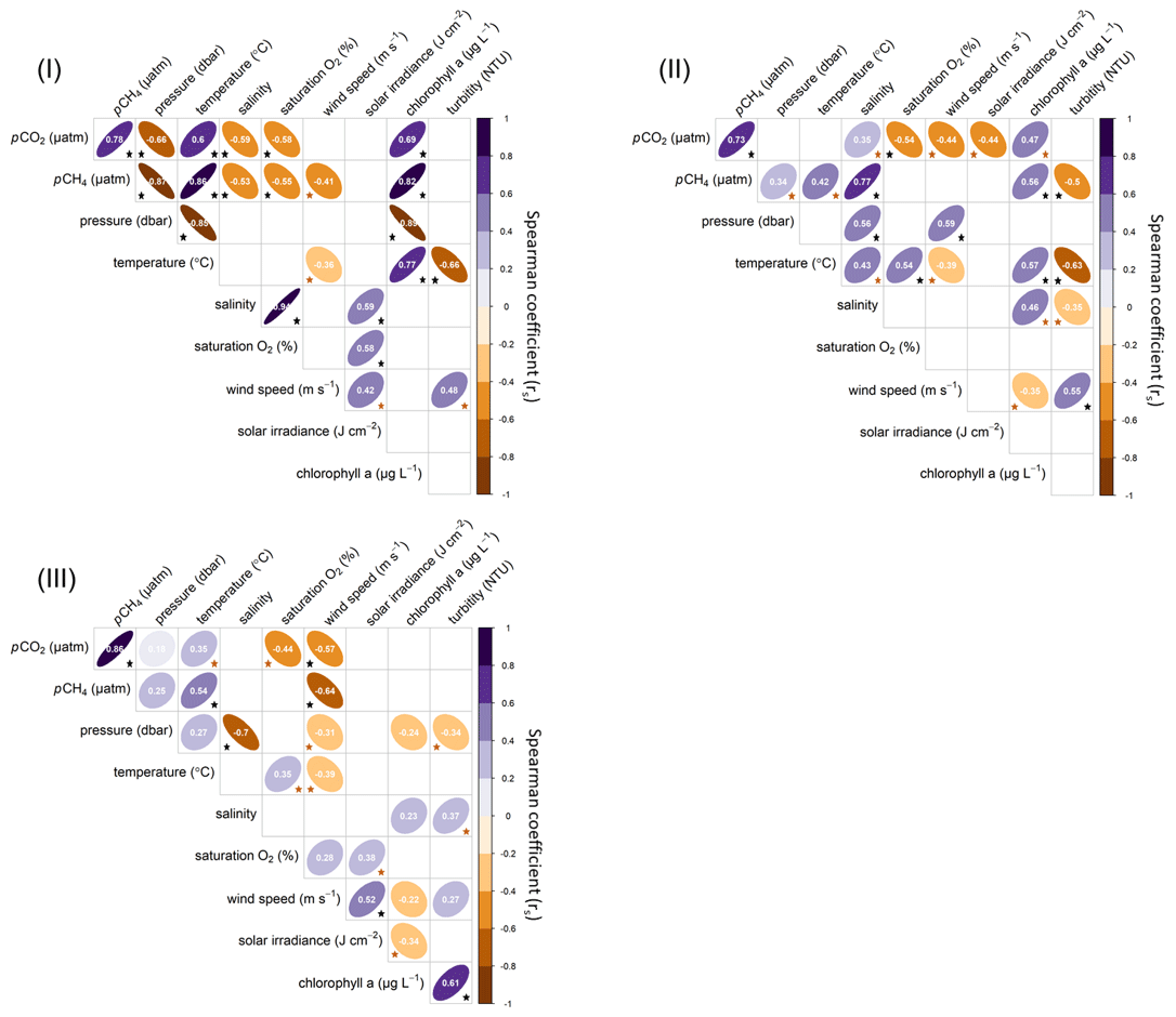
Figure E4 Spearman correlation coefficients (r_s) between the measured variables of lander 1, wind speed, and solar irradiance limited to the three time periods (I)–(III). A correlation level of 0.001 was used to remove non-correlating relationships (empty fields). In addition, the Cohen convention (Cohen, 1988) was used to interpret the effect size. The black stars represent a large effect size and thus a strong correlation, while the brown stars represent a medium effect size. Wind speeds were retrieved from the station Putbus (WMO-ID 10093) and solar irradiance from Rostock-Warnemünde (WMO-ID 10170; both DWD).

Appendix F: Discussion

F1 Assessment of the data quality and implications for future lander deployments

The direct comparison of the GHG partial pressures derived from the bottle data with the sensor measurements (calculated mean of ∼ 10 min prior to discrete sampling) showed good agreement in some cases but also large discrepancies, with differences ranging from −2.2 % to 445.3 % for pCO₂, and with higher discrepancies for the pCH₄ determinations, ranging from 11 % to 600 % (Table C1). This observation demonstrates the complexity of combining both approaches in such a challenging and heterogeneous environment. Reconciliation of discrete bottle data with continuous sensor data is complicated by a variety of potential influences due to​​​​​​​​ ​​​​​​​​ variable field conditions, a difficult sampling environment, and long sensor response times (Canning et al., 2021). For example, discrete sampling of water in such shallow water may lead to minor sediment disturbance (i.e., boat mooring, Niskin bottle movements). In addition, bottom water is very heterogeneous for microbial mediated processes in both lateral and vertical directions, and sampling directly at the pump basket or sensor inlet could not be performed satisfactorily. The effect of water heterogeneity was also noticeable in the duplicates of the bottle CH₄ data, with some varying by > 25 % (corresponding for several 100 nmol L⁻¹), even though the duplicates were from the same batch of Niskin bottle (data not shown). In future deployments, discrete sampling at the sensor inlet by an automated sampler should lead to a more reliable comparison. Still, the different nature of the data, including the smoothing effect of the sensor data even with a state-of-the-art time lapse correction, makes comparison difficult. The similarity of the major trends in the data series on both landers is a strong indicator of the quality of the data, and under unlimited resources, double sensor setups would always be very favorable.

The absolute numbers of a fraction of the data for pCO₂ and pCH₄ from the sensors have a small uncertainty because the selected calibration was exceeded partly (pCO₂), and the pumps did not run reliably over the entire period, resulting in a lower flux onto the membrane. A similar situation occurred with the CTD–O₂ measurement, resulting in parts of the data having to be discarded. These disturbances were related to the shallow water depths and high sediment transport and resulted in a lower data quality. Nevertheless, a robust post-processing was achieved, and hence presenting the data is valid because the natural heterogeneity is much more pronounced and they address the current scientific and policy issue of peatland rewetting. Moreover, the data provided a detailed insight into the biogeochemical processes in a rewetted peatland and addressed important topics in coastal research.

Improvements in future deployments can be achieved by adjusting the pumps. For example, all sensors should be equipped with a central inlet or revised pumps that are more resistant to environmental influences. In addition, more attention should be paid to controlling the water flow at the sensor units, such as by monitoring the flow or using self-cleaning pump systems. The use of additional non-pumped loggers, e.g., for CTD–O₂ determinations, can supplement and validate sensor data, and the fouling protection could be achieved by using UV light lamps. Furthermore, we plan to update and improve the real-time data transmission to respond quickly to lander system irregularities.

F2 Selected greenhouse gas emissions of CO₂ and CH₄ along the land–sea interface

Table F1 Selected greenhouse gas emissions of CO₂ and CH₄ along the land–sea interface in relation to the derived GHG fluxes from our study.

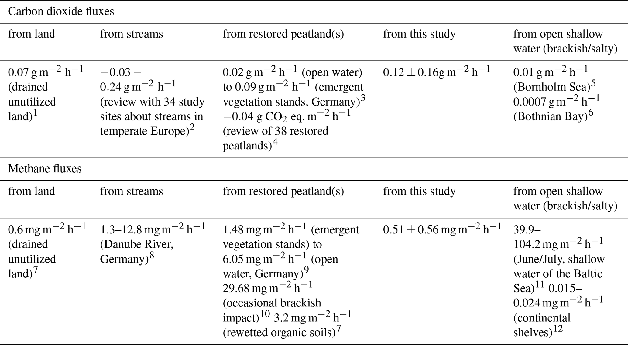
References for the partially adjusted numbers (as footnotes): ¹ Tiemeyer et al. (2020). ² Mwanake et al. (2023). ³ Franz et al. (2016). ⁴ Bianchi et al. (2021). ⁵ Thomas and Schneider (1999). ⁶ Löffler et al. (2012). ⁷ Tiemeyer et al. (2020). ⁸ Lorke and Burgis (2018). ⁹ Franz et al. (2016). ¹⁰ Hahn et al. (2015). ¹¹ Heyer and Berger (2000). ¹² Bange et al. (1994).