Can atmospheric chemistry deposition schemes reliably simulate stomatal ozone flux across global land covers and climates?

Over the past few decades, ozone risk assessments for vegetation have evolved two methods based on stomatal O₃ flux. However, substantial uncertainties remain in accurately simulating these fluxes. Here, we investigate stomatal O₃ fluxes across various land cover types worldwide simulated by six established deposition models. Hourly O₃ concentration and meteorological data at nine sites were extracted from the Tropospheric Ozone Assessment Report (TOAR) database, a comprehensive global collection of measurements, for the model simulations. The models estimated reasonable O₃ deposition (0.5–0.8 cm s⁻¹ in summer), which is mostly in agreement with the literature. Simulations of canopy conductance showed differences that varied by land cover type with correlation coefficients of 0.75, 0.80, and 0.85 for forests, crops, and grasslands among the models. Differences between models were primarily influenced by soil moisture and vapour pressure deficit, depending on each model's specific structure. Across models, the range of O₃ damage simulations at each site was most consistent for crops (6 to 11 mmol O₃ m⁻²), followed by forests (3 to 19.5 mmol O₃ m⁻²) and grasslands (7 to 33 mmol O₃ m⁻²). The median estimate across models aligns well with the literature at the sites most vulnerable to O₃ damage. Overall, this study represents a critical first step in developing and evaluating tools for broad-scale assessment of O₃ impacts on vegetation within the framework of TOAR phase II.

1 Introduction

Elevated surface O₃ levels significantly damage vegetation due to the stomatal uptake of O₃ by canopy leaves. Stomatal uptake of O₃ leads to plant tissue injury, which in turn causes changes in metabolic functioning, reducing photosynthesis and consequently plant growth and productivity (Mills et al., 2011; Emberson, 2020; Ainsworth et al., 2012; Fuhrer et al., 2016; Grulke and Heath, 2020). Such damage can have significant impacts on crop yields and quality, leading to economic losses and impacting food security in regions already facing scarcity (Avnery et al., 2011; Ainsworth, 2017; Ramya et al., 2023). There is an ever-growing body of observational evidence demonstrating a variety of O₃ impacts on different ecosystems (crops, forests, grasslands) in North America; Europe; and, more recently, Asia (Emberson 2020). Various indices assessing O₃ exposure to vegetation have been developed over recent decades, with the stomatal O₃ flux (POD_y; phytotoxic ozone dose over a threshold y) index found to provide better estimates of O₃ risk to vegetation than the more commonly used concentration-based exposure approaches (e.g. accumulated ozone over threshold (AOT); growing season daylight mean O₃ concentration (M7, M12), Mills et al., 2011; Avnery et al., 2011). A global overview of spatial distribution and trends using concentration-based metrics was provided in the first Tropospheric Ozone Assessment Report (TOAR) by Mills et al. (2018). During TOAR phase II (TOAR-II), we conduct a flux-based analysis to ensure the most up-to-date vegetation metrics are provided through this community effort.

O₃ dry deposition to vegetation is in part determined by canopy-level O₃ concentrations. A significant fraction of O₃ uptake occurs through the plant stomata with the remainder depositing on plant cuticular surfaces and the under-storey vegetation and soil. The stomatal contribution can vary between 50 % and 80 %, depending on the factors controlling the partitioning of stomatal and non-stomatal uptake (e.g. Huang et al., 2022; Wong et al., 2022; Clifton et al., 2023). As such, quantifying canopy stomatal conductance is important for assessing the mass balance of atmospheric O₃ concentrations and its potential damage to vegetation. Both stomatal and non-stomatal processes can vary with environmental conditions such as humidity, solar radiation, temperature, and CO₂ concentration as well as vegetation type and density (Clifton et al., 2020a). The occurrence of soil water deficit can also play a crucial role, where soil water stress induces stomatal closure (Li et al., 2020; Huang et al., 2022). There are two commonly used stomatal conductance (g_s) models – the empirical, multiplicative approach first developed by Jarvis (1976) and the semi-mechanistic coupled net photosynthesis–stomatal conductance models (A_net−g_s). The common Jarvis-type models (e.g. Emberson et al., 2000; Ganzeveld and Lelieveld, 1995; Zhang et al., 2003), widely applied due to their simplicity and computational efficiency, correct a prescribed maximum stomatal conductance with the multiplication of different environmental factors (e.g. temperature, light, soil water, and atmospheric moisture). The A_net−g_s models couple g_s to plant photosynthesis by calculating the net assimilation of CO₂ and estimating g_s based on the resulting supply and demand of CO₂ (Farquhar et al., 1980; Goudriaan et al., 1985; Ball et al., 1987). A_net−g_s models involve multiple non-linear dependencies on soil water, humidity, and temperature, among other factors defined by measurement constraints (Ball et al., 1987; Leuning, 1997). Heterogeneity of stomatal deposition estimates over different land cover types is anticipated, but model uncertainty depends on the representation of the deposition mechanisms, model parameterization, and meteorological inputs (Hardacre et al., 2015; Clifton et al., 2020b; Huang et al., 2022; Khan et al., 2025). Broadly speaking, the pros and cons of these two modelling approaches will tend to depend on the aims of the risk assessment study, the extent of knowledge of the ecosystem being investigated and prevailing bio-climatic conditions. Jarvis-type models are arguably more suitable for studies where less is known about the eco-physiology of the ecosystem since they do not require simulation of net photosynthesis, which in itself is inherently difficult to model accurately. However, these models still need to be calibrated for the particular bio-climate of study to ensure temperature and vapour pressure deficit (VPD) functions are suitable for the prevailing conditions. By contrast, A_net−g_s models may be more useful for studies where the physiological response to environmental conditions of the ecosystems is reasonably well understood as they can provide insight into not only pollutant deposition but also how other environmental conditions in addition to pollution may limit plant growth and productivity more generally.

In this study, the stand-alone versions of six O₃ deposition schemes, commonly used in climate or air quality models, are assessed, with a focus on their stomatal uptake portion and resulting POD_y calculation. Using concurrent O₃ concentration and meteorological variable measurement data from the TOAR database enables us to conduct a detailed intercomparison of multiple deposition schemes by avoiding uncertainties arising from using different input data. For this study, various sites have been selected to represent different land cover types and climate regimes around the globe, focusing on sites where observational data are available for O₃ concentration. By assessing the model estimates of stomatal O₃ deposition at these different sites, we aim to identify key differences in model formulation and parameterization that influence estimates of stomatal O₃ flux and consequent POD_y. The estimation of the stomatal uptake from water flux measurements taken from the FLUXNET database provides an additional observational constraint as well as an uncertainty estimate at each site.

Furthermore, sensitivity simulations allow us to investigate the variability of stomatal O₃ deposition and plant damage with key input parameters and land cover characteristics. Post hoc, plant damage will be calculated offline based on the POD_y simulated by different models and flux–response relationships, where appropriate. Ultimately, we aim to understand the key factors driving stomatal O₃ flux and thus POD_y and assess the O₃-induced potential for vegetation damage for different land cover types and global regions.

2 Methodology

2.1 Meteorological and O₃ data from the TOAR-II database

The web version of the DO₃SE model is coupled to the TOAR database; i.e. the required input data (Table 3) are automatically provided by the database at the respective modelling sites. The TOAR-II database (from now on TOAR) contains harmonized measurements of surface O₃ and its important precursors and key meteorological variables that can impact O₃ concentrations and stomatal O₃ uptake. As one of the largest collections of quality-controlled air pollution measurements in the world, it comprises ground-based station measurements of O₃ concentration at more than 22 905 sites globally, which cover different periods between 1974 and 2023. These have been collected from different O₃ monitoring networks (e.g. Clean Air Status and Trends Network, CASTNET), harmonized and synthesized to enable uniform processing. The data were selected for inclusion in the TOAR database based on an extended quality control; e.g. sites where the measurement technique changed with time have been excluded. Data errors remain but have been shown to have a minor impact (Schultz et al., 2017). The total uncertainty in modern O₃ measurements is estimated to be <2 nmol mol⁻¹ (Tarasick et al., 2019). The meteorological data (irradiance, air temperature, relative humidity, precipitation, air pressure, and wind speed) in the database stem from the fifth generation of ECMWF reanalysis (ERA5) for global climate (Hersbach et al., 2020). Data re-initialization (of precipitation and radiation, Copernicus Climate Change Service, 2017) is bridged by (linear) interpolation. The leaf area index (LAI) data in the database stem from the MODerate resolution Imaging Spectroradiometer (MODIS). TOAR data are freely and openly available through a graphical user interface and a representational State Transfer interface (https://toar-data.fz-juelich.de/api/v2/, last access: 1 November 2024). The TOAR data centre team is committed to the Findability, Accessibility, Interoperability, and Reusability principles (Wilkinson et al., 2016). The centre aims to achieve the highest standards regarding data curation, archival, and re-use (Schröder et al., 2021). To conduct offline simulations with models in addition to Web-DO₃SE, the input data were extracted beforehand and proven for identicality. The additionally required data (Table 3) were extracted from the TOAR database and the MeteoCloud server (https://datapub.fz-juelich.de/slcs/meteocloud/index.html, last access: 21 September 2024) at Forschungszentrum Jülich.

2.2 Observation-constrained stomatal conductance

To compare the modelled stomatal conductance with observational information, we prepared model input data at two sites (Hyytiälä, Harvard Forest) from the FLUXNET 2015 dataset (Pastorello et al., 2020), which is openly available under the CC-BY-4.0 data usage license. Additional vegetation information for the model input (i.e. LAI, canopy height, and crop calendar data) was provided by the site project investigators. Then, we used the canopy-scale stomatal conductance dataset, SynFlux version 2, to estimate G_st for two forest sites, US-Ha1 and FI-Hyy. While in SynFlux version 1, canopy transpiration is assumed to be equal to total latent heat flux, SynFlux version 2 improved its previous estimations (Ducker et al., 2018) using a machine-learning-based method (Nelson et al., 2018) to partition total evapotranspiration into surface evaporation and canopy transpiration. To train quantile random forest models to relate meteorological conditions with water use efficiency (derived from water and carbon fluxes), periods with minimal surface wetness were chosen during the growing season. These models were then used to back-calculate transpiration for the whole growing season. Instead of the total latent heat flux, the resulting transpiration estimate was used as an input to the inverse Penman–Monteith equation, reducing the potential high bias in the stomatal conductance estimates in SynFlux version 1.

2.3 Summary of sites selected for deposition modelling

Nine sites (Table 1) were selected for this modelling work accounting for the following factors: (i) geographical spread, including major continents with terrestrial vegetation; (ii) land cover/use types, including the plant functional types (PFTs) which are important in terms of economy, food security, or biodiversity and for which we have fairly good knowledge of O₃ impacts; (iii) availability of meteorological and O₃ data from the TOAR database; (iv) availability of observational data describing stomatal conductance of water vapour (g_wv) estimated from the FLUXNET measurements (Sect. 2.2); and (v) location proximity to previous experiments that have investigated O₃ impacts on vegetation that can help interpret our model results.

Table 1 Sites selected for stomatal deposition modelling using data from the TOAR database grouped by continent. Sites that also have FLUXNET data are denoted by “FN”, and those with SynFlux data are denoted by “SF”.

Table 2 Land cover type, species, and growing season (where SGS: start of growing season and EGS: end of growing season) by site. The equivalent land cover type and soil texture data used by the models used in this study (Sect. 2.3) are also shown. MESSy does not consider different land cover types. Models that do not consider soil type (i.e. do not include an estimate of soil moisture influence on stomatal deposition) are marked with *.

Figure 1 Locations of nine selected sites on Köppen–Geiger climate classification map for 1991–2020 (source: Beck et al., 2023). Table 1 specifies the classifications of these sites. Publisher’s remark: please note that the above figure contains disputed territories.

2.4 Stomatal deposition models and their key inputs

Six widely used empirical/Jarvis and semi-empirical/Ball–Berry types of stomatal deposition models were selected for this study. All of these used models can accommodate a variety of land cover/land use types and provide estimates of stomatal deposition that can be output as both hourly- and season-long cumulative-stomatal deposition metrics. The key model features are described below.

1. The empirical/Jarvis-type models use a predefined stomatal conductance modified with different environmental stressors for radiation (PAR), air temperature (T), vapour pressure deficit (VPD), and soil water (SM): the ZHANG model (Zhang et al., 2002, 2003) and the Web-DO₃SE model (i.e. a version of DO₃SE that is directly coupled to the TOAR database, Emberson et al., 2000) account for sunny and shaded leaves (two big leaves), and the Web-DO₃SE model also depends on the vegetation phenology. The CMAQ_J model (Pleim and Ran, 2011) and the MESSy model (Ganzeveld and Lelieveld, 1995; Kerkweg et al., 2006) account for one big leaf. CMAQ_J uses relative humidity (RH) instead of VPD. MESSy calculates the initial stomatal conductance based on the PAR and several empirical parameters.

2. Semi-empirical/Ball–Berry: the CMAQ_P model (Ran et al,. 2017) and the TEMIR model (Collatz et al., 1991; Farquhar et al., 1980) calculate the stomatal conductance at sunlit and shaded leaves for C₃ and C₄ plants depending on the net CO₂ assimilation rate, CO₂ partial pressure, atmospheric pressure (Pa), and water vapour pressure for each leaf. The NOAH-GEM model is different, calculating stomatal conductance for one big leaf using RH instead of VPD (Wu et al., 2011; Niyogi et al., 2009).

All models follow the resistance scheme.

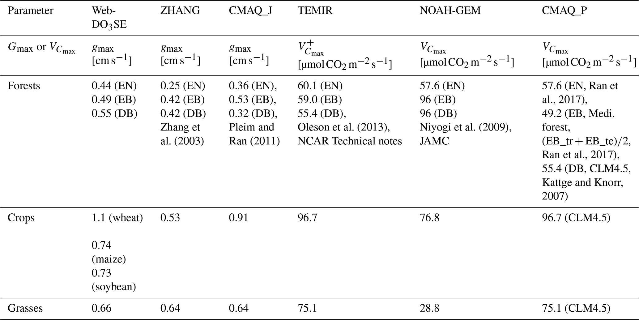
The land cover, growing season, and soil texture specifications used by the models are summarized in Table 2. For crops, we used the GGCMI Phase 3 crop calendar (Jägermeyr et al., 2021a), which provides the planting date and maturity day for 18 different crops at a 0.5° land grid cell resolution (Jägermeyr et al., 2021b). For forest trees, we consider four various classes: evergreen needleleaf (EN), evergreen broadleaf (EB), deciduous needleleaf (DN), and deciduous broadleaf (DB). For evergreen species, we assume a year-round growing season; for deciduous species, we use the simple latitude function described in Hayes et al. (2007); and we consider a year-round growing season for tropical species. The soil texture categories used by the models were obtained from the reference studies in Table 1 and the site principal investigators. Table 3 provides the key formulas, input data requirements, and references for all models. Key total and stomatal deposition parameters for empirical models (g_max) and semi-empirical models ($V_{C_{\max }}$) are described in Table 4, which gives a good indication of the overall difference in the magnitude of stomatal deposition. The models' meteorological and O₃ inputs have been introduced in Sect. 2.1.

Table 3 Stomatal deposition models selected for site-scale modelling (list of symbols: A1 and Sect. S3 in the Supplement, * uses u(h), o3(h)=1, for US-Ne: u(h), o3(h)=0.3).

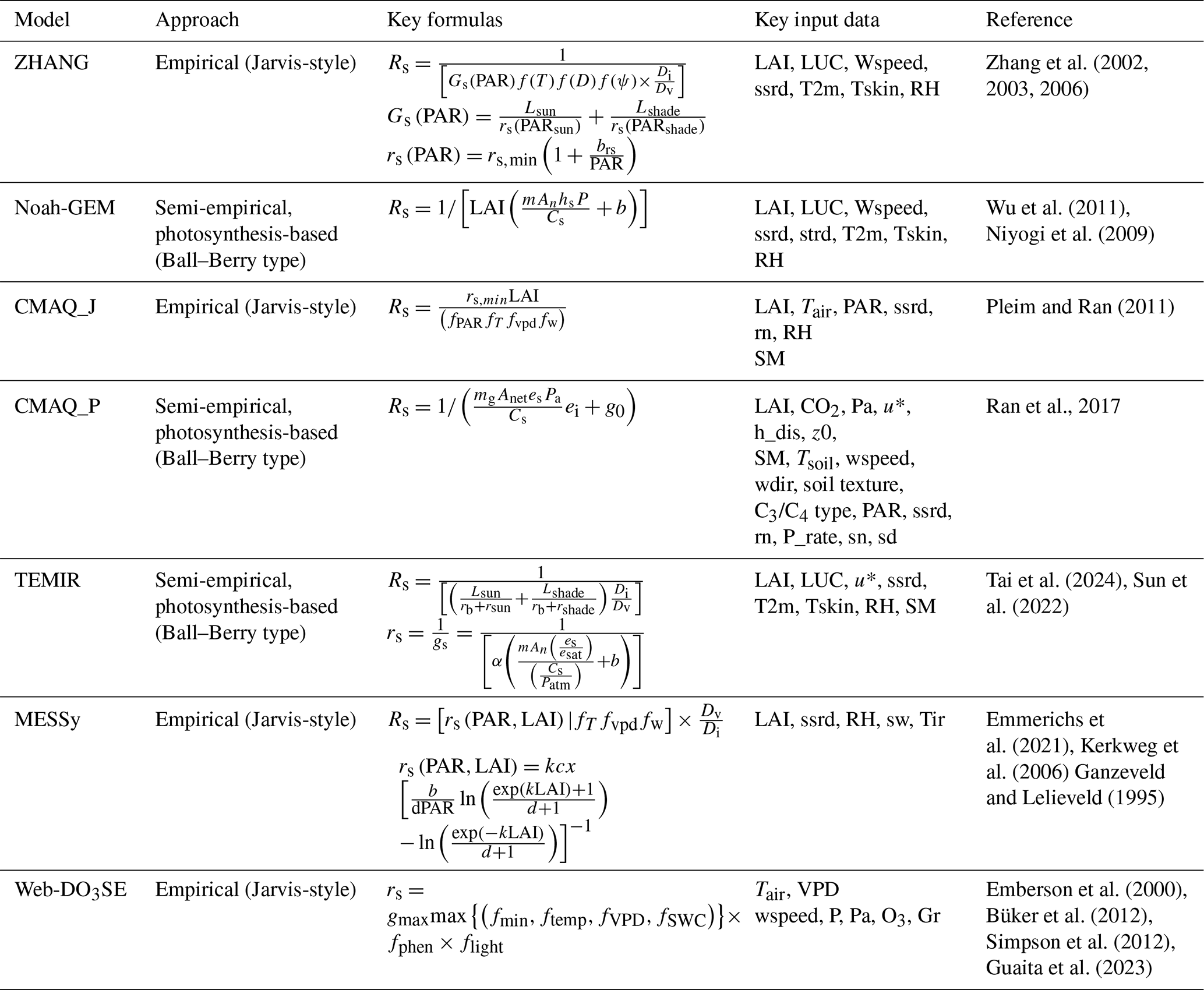
Table 4 Model parameter $V_{C_{\max }}$ at standardized temperature conditions (25° C) [in $\mathrm{\mu }\mathrm{mol}{\mathrm{CO}}_{\mathrm{2}}{\mathrm{m}}^{-\mathrm{2}}{\mathrm{s}}^{-\mathrm{1}}$] and g_max [O₃ in cm s⁻¹] for the total canopy by land cover/land use type. Note that the values presented in the table were recalculated from the original respective rsmin values for H₂O (s m⁻¹) in ZHANG, MESSy, and CMAQ_J and $V_{c_{\max }}$ values for O₃ (mol O₃ m⁻² s⁻¹) in Web-DO₃ SE.

POD_y is calculated in post-processing, according to the guidelines in UNECE LRTAP (2017):

$$\begin{array}{}\text{(1)}& \begin{array}{rl}& {\text{POD}}_y={\sum }_{i=\mathrm{1}}^n\left[\text{fs}t,{\mathrm{sun}}_i-y\right]\times \left({\displaystyle \frac{\mathrm{3600}}{{\mathrm{10}}^{\mathrm{6}}}}\right)\\ & \text{for fs}t,{\mathrm{sun}}_i\ge y\mathrm{nmol}{\mathrm{m}}^{-\mathrm{2}}\mathrm{PLA}{\mathrm{S}}^{-\mathrm{1}},\end{array}\end{array}$$

where fst,sun_i is the hourly mean O₃ flux in nmol O₃ m⁻² PLA s⁻¹ at sunlit leaves, y is a species-dependent threshold (crops: 6 nmol O₃ m⁻² s⁻¹, grassland and forests: 1 nmol O₃ m⁻² s⁻¹; UNECE LRTAP, 2017), and i is the number of daylight hours (when ssrd >50 W m⁻²) within the accumulation period (growing season). The term ($\mathrm{3600}/{\mathrm{10}}^{\mathrm{6}}$) converts from nmol m⁻² PLA s⁻¹ to mmol O₃ m⁻² PLA. fst,sun is calculated by

$$\begin{array}{}\text{(2)}& f_{\mathrm{st},\mathrm{sun}}=c{\displaystyle \frac{\left(z\right)\times g_{\mathrm{st}}\times r_{\mathrm{c}}}{r_{\mathrm{b}}+r_{\mathrm{c}}}},\end{array}$$

where c(z) is the O₃ concentration at in nmol m⁻³ , calculated from ppb by multiplying by $P/RT$, where P is the atmospheric pressure (Pa), T is the air temperature (K), R is the universal gas constant of 8.31447 J mol⁻¹ K⁻¹, and T is the assumed standard air temperature (293 K). The leaf surface resistance (r_c) is given by $r_{\mathrm{c}}=\mathrm{1}/(g_{\mathrm{st}}+g_{\mathrm{ext}}$), where g_ext is the inverse of cuticular resistance.

The leaf boundary resistance is calculated by

$$\begin{array}{}\text{(3)}& r_{\mathrm{b}}=\mathrm{1.3}\times \mathrm{150}\times \sqrt{{\displaystyle \frac{L}{u\left(h\right)}}},\end{array}$$

where factor 1.3 accounts for the differences in diffusivity between heat and O₃, L is the crosswind leaf dimension (i.e. leaf width in m), and u(h) is the wind speed at the top of the canopy.

2.5 Description of stomatal deposition model simulations

The result section aims at identifying trends in stomatal deposition models among different land cover types including grass, crops, and forests using four model experiments as follows.

In experiment 1, the different models are driven by the O₃ and meteorological data from ERA5. We analysed the simulated deposition velocity (V_d) split into stomatal and non-stomatal fractions, canopy (G_st) and sunlit (G_sun) stomatal conductance.

To include observational constraints, in experiment 2, the TEMIR, ZHANG, NOAH, MESSy, and CMAQ models were run with data obtained from the FLUXNET database (available for three sites; see Table 1), and the simulated G_st was evaluated with observation-derived values, inferred G_st, of SynFlux. Spearman correlation was applied for the model evaluation, as it can be applied to any datasets including non-parametric and non-linear ones. The US-Ha1 and FI-Hyy sites were considered for the model evaluation due to the availability of SynFlux data at these sites.

A sensitivity analysis (experiment 3) was performed by driving a set of models with synthetic input data in the following steps: (i) O₃ input was perturbed by ±40 % (Sofen et al., 2016). (ii) Soil water content was perturbed by ±30 % (Li et al., 2020). (iii) Absolute humidity was perturbed by ±30 %, and soil and air temperatures were perturbed by ±3, independently. (iv) The growing season, which was mostly approximated by LAI, was shifted by 14 d forward and backward in time. In set (iii) and (iv), relative humidity was calculated from absolute humidity and temperature after their perturbation. In both cases, absolute humidity was capped at the saturation vapour pressure at the corresponding temperature.

Finally, for experiment 4, g_max and $V_{C_{\max }}$ of the models were varied by ±20 %, based on previous estimates of plant-trait-dependent uncertainty (e.g. Walker et al., 2017; UNECE LRTAP, 2017).

3 Results

3.1 General characteristics of simulated total deposition velocity and stomatal contribution

The split of total O₃ deposition between different pathways, G_st, G_cut, and G_ground, simulated by the seven models, is shown for each of the nine sites in Figs. 2 and S2 (corresponding data are presented in Table S9). This analysis allows us to briefly assess the overall efficacy of the model's ability to simulate deposition velocity V_d (by comparisons with previously published values; more complete assessments of model's ability for some of these sites can be found in Clifton et al., 2023) and to compare the importance of the stomatal deposition pathway between models for different land cover types and across different seasons.

Observations of V_d have only been made at a handful of sites, i.e. Hyytiälä, Finland; Castelporziano, Italy; Grignion, France; and Harvard Forest, USA (close to our Quabbin site in terms of proximity, land, cover type and climate). Overall, the models capture V_d at these sites compared to observed values reported in previous studies. Namely, the observed seasonal cycles in V_d at Hyytiälä, Finland (needleleaf forest), with lows of ∼0.1 cm s⁻¹ between January and April and highs of 0.4 cm s⁻¹ between June and September, averaged over 10 years of measurements from Clifton et al. (2023) and Visser et al. (2021) are captured by most models except MESSy and TEMIR, which reach V_d values of 0.8 cm s⁻¹ during the summer. Similarly, the strong seasonal cycle in V_d at Quabbin, USA (temperate mixed forest), ranging from around 0.2 cm s⁻¹ between January and April up to 0.5 cm s⁻¹ from June to September in Clifton et al. (2023), is captured by all models. Observed V_d at Castelporziano, Italy (evergreen broadleaf forest), shows relatively constant values throughout the year, commonly between 0.4 and 0.8 cm s⁻¹ averaged over a 2-year period (Savi and Fares, 2014). The study by Stella et al. (2011) reports V_d measurements of 0.63 cm s⁻¹ (on average) at Grignion (France). At the other sites, no O₃ dry deposition measurement exists, and thus we report the observed ranges for the land cover type (and possibly the matching climate). Over grassland, Silva and Heald (2018, and references therein) show a mean of 11 measurements of daytime V_d values (∼0.4 cm s⁻¹) in agreement with our models. Measurements exist at soybeans and maize crops which indicate V_d values of 0.7 (Meyers et al., 1998) and 0.4–0.6 cm s⁻¹ (Stella et al., 2011), respectively. Thus, the models seem to estimate too low deposition at soybeans.

In terms of deposition pathways, for all sites and models, stomatal deposition consistently ranks as the most important pathway in the summer, whereas in winter and, for some models, in the autumn G_st decreases to zero to very low at sites with seasonal variation in vegetation coverage. The importance of the pathway varies with land cover type and season. The highest stomatal contribution of 90 % (NOAH model) is shown at the Amberd site. Among the different land cover types, the highest average stomatal contribution to deposition during the summer is estimated across grass (67 %), followed by crops (65 %) and forests (59 %). The seasonal importance of stomatal contribution is not seen for the tropical sites as the year-round growing season means that stomatal conductance is driven by solar radiation, which is constant throughout the year (e.g. Hardacre et al., 2015). Previous studies involving measurements and partitioning approaches (Horváth et al., 2018; Mészáros et al., 2009) indicate that the non-stomatal O₃ deposition pathways (i.e. G_ground and G_cut) are very strong (in some cases, dominant over G_st) at short vegetation such as the grasslands. Despite there being multiple factors, such as wind speed, solar radiation, and LAI, which control the relative contributions of the three deposition branches, G_st is the dominant pathway at the three grassland sites of the current study (Amberd, Mt. Kenya, and Peru). At the Amberd and Peru sites, G_cut and G_ground are small since low wind speed reduces downward mixing of ozone to the surface (atmospheric resistance; e.g. at the Peru site in the summer season, the mean wind speed was 1.0 cm s⁻¹, and the G_cut and G_ground contributions in the TEMIR model were 21 % and 12 %, respectively; Table S3).

In contrast, at the Mt. Kenya site, G_st exceeds G_cut and G_ground, since the strong solar radiation (annual mean is 246 W m⁻², Table S2) at this site favours stomatal opening. Besides that, LAI is a very important governing factor for G_st. Therefore, it can be inferred that the O₃ deposition pathway depends on not only the land cover type but also meteorological drivers. The relative contribution of each deposition pathway depends on the interplay between these key factors at a particular site. Among the models, Web-DO₃SE estimated the lowest stomatal contribution at grass (Fig. 2) most likely due to its parallel pathways to cuticle, soil, and stomata, with the former scaled by LAI with a constant cuticular deposition of 2500 s m⁻¹. Such differences in model structures likely led to the wide-ranging partitioning. For example, for the Quabbin site (summer), all models simulate G_cut ranging from 15 %–65 %, G_ground from 2 %–19 %, and G_st from 33 %–66 % despite their agreement on the overall V_d values (total bar). Models agree better in the partitioning of O₃ dry deposition to crops, with summer stomatal fraction contributions ranging between 46 %–73 %, 37 %–73 %, and 51 %–81 % for US-Ne3 Maize, US-Ne3 soybeans, and FR-Gri (rapeseed and wheat). Most models estimate non-stomatal deposition equal to or larger than the stomatal contribution to deposition outside of the tropics in winter and autumn and to some extent in spring. This again emphasizes the importance of the stomatal contribution to the seasonal cycle of total deposition as also found in Clifton et al. (2023). Similarly, as seen at grasslands, Web-DO₃SE (Fig. 2, Table S3) accounts for the highest non-stomatal deposition at crop sites.

Across all forest sites, models show significant cuticular uptake throughout the year ranging between 11 % and 94 % contribution. At FI-Hyy, G_cut averages ∼50 % across all seasons and all models with higher estimates of ∼55 % by the TEMIR model due to the higher wind speed at FI-Hyy (annual mean wind speed is 3.2 m s⁻¹; Table S2), favouring cuticular deposition as suggested by Rannik et al. (2012). At IT-Cpz, our models estimate on average around 43 % (20 %–80 %) to be non-stomatal deposition, close to the previously reported ranges (Gerosa et al., 2005; Fares et al., 2012, 2014), which were up to 57 % from non-stomatal deposition and 30 %–60 % from stomatal uptake. A similar partitioning (59 % G_st, 33 % G_cut, 5 % G_ground model average in summer) is seen at PhaDin.

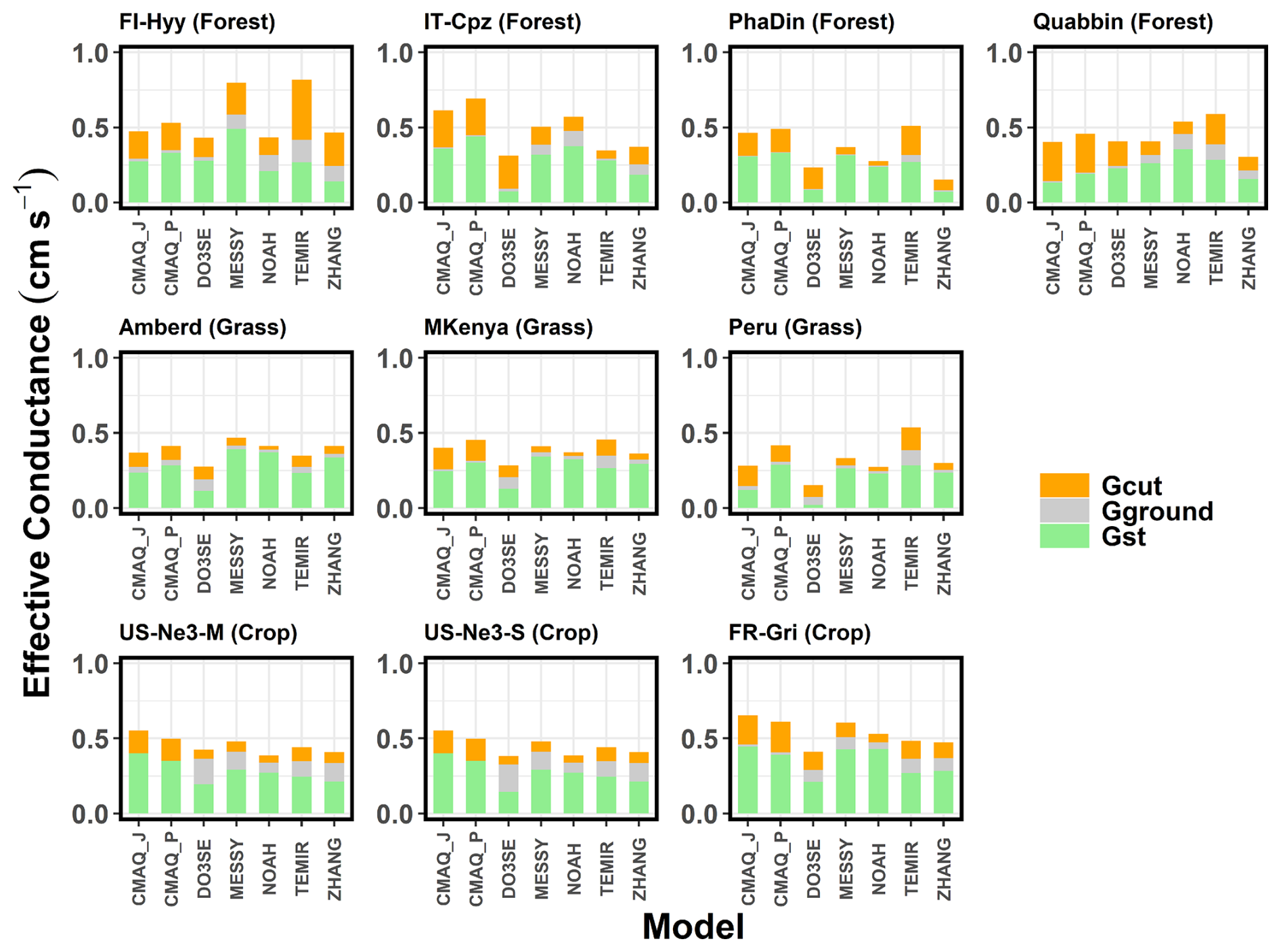
Figure 2 Mean effective conductance of the cuticular (G_cut), ground (G_ground), and stomatal (G_st) deposition pathways of O₃ across various models and sites during the summer season (US-Ne3-S = soybeans, US-Ne3-M = maize). Respective figures for the other seasons are presented in the Supplement.

All models except Web-DO₃ SE were compared on a seasonal and hourly basis with the SynFlux G_st data for US-Ha1 and FI-Hyy sites (Figs. S2, S3). CMAQ_J, NOAH, TEMIR, and ZHANG show reasonable agreement at the Quabbin forest (US-Ha1), whereas CMAQ_P and MESSy show quite significant overestimates at both FI-Hyy and Harvard Forest (Table S5) and CMAQ_J overestimates at FI-Hyy only. Note that NOAH and ZHANG show significant underestimates at FI-Hyy while agreeing well with SynFlux at Harvard Forest (Quabbin). The underestimates by the ZHANG model are consistent with the results from a similar comparison for Yellowstone National Park in the USA by Mao et al. (2023). Compared to Harvard Forest, FI-Hyy is the most humid and cloudy with the lowest solar radiation flux, and these conditions likely contribute to the underestimates by the NOAH and the ZHANG model as identified by Mao et al. (2023). The differences between modelled and SynFlux G_st do not seem to be associated with the model types, i.e. empirical or photosynthesis-based models.

The correlation of the diurnal cycle of G_st calculated by the models with the inferred G_st by SynFlux for US-Ha1 and FI-Hyy (Fig. S4) confirms that models generally capture the temporal patterns of G_st of at least these two different forest types and climates (FI-Hyy: EN, temperate, subarctic; Quabbin: DB, moist temperate). The best Spearman correlations are found at FI-Hyy and range between 0.73 by the MESSy model and 0.85 by the TEMIR model. Overall lower correlations are found at the Quabbin site ranging from 0.65 for the NOAH and MESSy models to 0.82 for the CMAQ_P model. This poorer correlation suggests that additional water stress may limit stomatal conductance at Quabbin, which the models do not capture, compared to FI-Hyy. Notably, a similar range of correlation coefficients (0.61–0.93) was found when modelled G_st values obtained using the TOAR input data were compared with SynFlux G_st. As SynFlux data were generated using FLUXNET measurement data, this result corroborates the validity of using the TOAR database as input to Web-DO₃SE, developed as a service website to aid in risk assessment of O₃ damage to European vegetation.

To identify the key drivers of the G_st model schemes among different land cover types and climate conditions, we also compare estimates of G_st between models for all sites and analyse the similarity of G_st diurnal cycles in empirical and photosynthesis models. Here, it is important to understand the model distinction between shaded and sunlit leaf (G_sun, Fig. 4). The average diurnal variations of stomatal conductance (G_st) of O₃ at the 9 sites for each season are shown in Figs. 3 and S7. This also helps interpret the modelled stomatal conductance of sunlit leaves (G_sun) shown in Figs. 4 and S8. Across all models, the diurnal mean G_st (Fig. 3) varied from 0.15 cm s⁻¹ (Quabbin) to 0.50 cm s⁻¹ (Mt. Kenya). In the TEMIR and the ZHANG model, roughly 50 % of G_st occurs at the sunlit part of the leaves. Web-DO₃SE and CMAQ_P G_sun contribute 30 % on average (Fig. 4). At middle to high latitudes, the model spread is limited to the summer season, whereas at tropical sites, it is similar throughout the year. During the day, models show a spread of 1.2 cm s⁻¹ in G_st at the forest and grassland sites during the summer, while their predictions agree most at the crop sites (throughout the year) with a maximum of 1.0 cm s⁻¹. This is due to the flux–response relationship, which has a more sensitive response (steeper slope for most crops) due to a higher threshold (see Table 5 for the equations describing the steepness of the change). Results among the same model type differed significantly, while different model types could produce similar results at the same location. For the sites with distinct seasonal variations, model differences were the largest in summer.

In comparison, TEMIR and ZHANG, photosynthesis-based and Jarvis-style, respectively, are both governed mainly by solar radiation (see higher G_sun in Fig. 4), showing close agreement, except in summer, at the forest sites (ZHANG values are very low). Only these two show a midday depression in G_sun at the peak of solar radiation at Mt. Kenya (the site with the highest radiation). The ZHANG model also estimated this feature for G_sun and G_st at other grassland sites (Figs. 3 and 4). This feature could be due to the day length (seasonality) scaling of $V_{C_{\max }}$ in TEMIR, causing G_st to increase significantly during summer at higher-latitude sites. In contrast, at lower-latitude sites (Mt. Kenya and Huancayo, Peru), the seasonal variation in day length is smaller, and there is subsequently smaller seasonality in $V_{C_{\max }}$ and G_st. The TEMIR and the CMAQ_P models, both photosynthesis-based, estimate very similar G_sun values (Fig. 4) at PhaDin (autumn, winter), IT-Cpz (spring, summer), and FI-Hyy (summer), whereas the G_st estimates show significant differences. The opposite occurs at Quabbin, where the G_sun values of the two models differ much more than the G_st estimates. These results illustrate that the different fractionations between shaded and sunlit leaves could mainly contribute to the model spread in stomatal conductance.

Further examination of individual models' features can shed light on the causes of model/site differences in G_st. The MESSy G_st value is strongly governed by LAI followed by soil moisture, and in all other respects MESSy treats different land cover types the same. Therefore, MESSy simulates the highest G_st values at PhaDin, Grignion, and Mt. Kenya, with LAI values of 6.9, 4.3, and 4.2 m⁻² m⁻², respectively (Table 1). In contrast to PhaDin, the high LAI site IT-Cpz (6.9 m⁻² m⁻²) experiences significant water stress during summer. This is only captured by MESSy and NOAH, indicating higher sensitivity to water stress. During the day, an evident midday depression of G_st due to hot weather and water shortage is seen, accompanied by a peak in the early morning evident from NOAH, the same as what has been observed in Mediterranean ecosystems (e.g. Gerosa et al., 2005). The NOAH model accounts for the direct effect of relative humidity on G_st (see model description in the Supplement) and subsequently modelled a depression in G_st at the daily onset (08:00 a.m. LT). This variation explains the G_st peak at IT-Cpz and Quabbin, which are, especially in the summer, the two driest among all sites. Due to the dry conditions at the Quabbin site, low soil water, and low relative humidity, most models, except NOAH, simulate the lowest summer daily mean G_st values among all sites. The high estimate by the NOAH model can be explained by the highest $V_{C_{\max }}$ value among the photosynthesis models (Table 4). The high g_max value of 0.55 cm s⁻¹ used in Web-DO₃SE leading to large estimates is largely dampened by strong soil moisture stress at IT-Cpz (Table S2). Similarly, Web-DO₃SE estimates the lowest G_st (among the models) values at the Peru site (grassland) due to a strong limitation by the f_temp function on stomatal conductance, suggesting that the minimum temperature for stomatal opening at 12 °C is too low for these cool temperate conditions. The ZHANG estimates are generally governed by g_max, explaining the highest and lowest G_st values of all models simulated with the ZHANG model at grassland and forest sites, respectively. The CMAQ_J model has the lowest g_max values, but it is strongly impacted by soil moisture. The additional dependence of the ZHANG model on solar radiation is reflected in higher G_sun relative to G_st (Figs. 3 and 4). TEMIR also simulates the smallest spread of G_st among the three grassland sites (Ambred, MKenya, Peru), as temperature acclimation of photosynthesis (Kattge and Knorr, 2007) is implemented. The different temperatures among the three sites have smaller effects on photosynthetic capacity and G_st than other models. Despite explicitly considering soil water stress, TEMIR does not capture the impacts of water stress on G_st in IT-Cpz and Quabbin in the summer, as the equivalent soil moisture threshold to trigger soil water stress at IT-Cpz and Quabbin is very low (<0.1 m⁻² m⁻³). Both versions of CMAQ respond very strongly to soil moisture, which may not be accurate for each site. The differences between CMAQ-J and CMAQ-P are greatest at the sites with the greatest LAI, such as IT-Cpz and PhaDin.

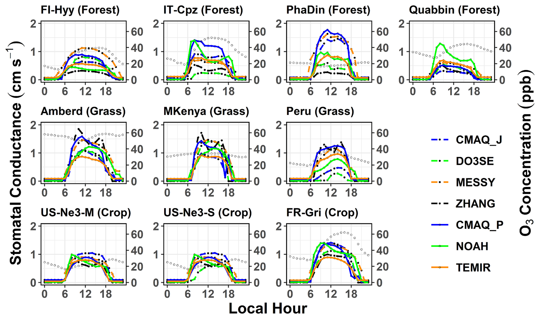
Figure 3 Mean diurnal cycle of total stomatal conductance (G_st) from models across various sites during the summer season (US-Ne3-S = soybeans, US-Ne3-M = maize). Open circles indicate diurnal O₃ variations. Respective figures for the other seasons are presented in the Supplement.

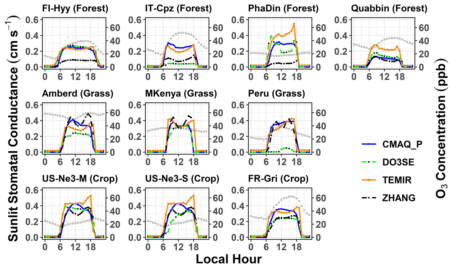
Figure 4 Mean diurnal cycle of leaf-level sunlit stomatal conductance (G_sun) from the three two-leaf models (CMAQ_P, TEMIR, and ZHANG) across various sites during the summer season (US-Ne3-S = soybeans, US-Ne3-M = maize). Open circles indicate diurnal O₃ variations. Respective figures for the other seasons are presented in the Supplement.

The difference between total and sunlit stomatal flux is examined, and trends of stomatal sunlit flux are characterized by different land cover types and climate conditions. Figures 5 and 6 show the (SRAD >50 W m⁻²) stomatal O₃ flux (F_st) and stomatal, sunlit O₃ flux (F_st,sun) for different models per season at nine sites representing forest (top), grass (middle), and crops (bottom). Thereby, we consider whether G_st and O₃ concentration co-variate at diurnal and seasonal timescales. Across all land cover types, a large range of F_st (0.05–2 ppb m s⁻¹, Fig. 5) is estimated, usually highest in spring and summer and lowest in winter. The largest median of F_st is found at Amberd (0.75 ppb m s⁻¹; ZHANG, summer), followed by IT-Cpz (0.60 ppb m s⁻¹; NOAH, spring), and FR-Gri (0.60 ppb m s⁻¹; MESSy and NOAH, summer), owing to both higher G_st and O₃ concentrations at the respective sites (Fig. 3). Consequently, no general trend can be identified among the sites; i.e. flux estimates can differ within one land cover type. Namely, the two crop sites show very different F_st estimates (Fig. 5) since they have the most different O₃ levels across one land cover type. The FR-Gri site is exposed to an annual mean O₃ of 45 ppb (Table S1); the lowest O₃ level is 25 ppb among all sites. The same applies for the diurnal variation of O₃, causing either a high (FR-Gri) or a low range (US-Ne3) of flux estimates among all models (in summer and spring). The difference is less apparent in the F_st,sun estimates (Fig. 6) which point to the sensitivity of the two leaves to O₃ concentration. Similarly, as seen for the stomatal conductance, three of four models show a very good agreement of F_st and F_st,sun among each other. In terms of seasonality, models agree also generally well among the grassland sites. Among those (and all land cover types), the maximum annual median F_st,sun was estimated for Amberd attributed to the high daytime (07:00 a.m.–07:00 p.m. LT) annual O₃ concentrations (49.3 ppb, Table S1). The most different F_st,sun (and F_st,sun) values are found between the ZHANG (highest) and Web-DO₃SE model (lowest) due to the difference in G_sun (Fig. 4). Web-DO₃SE disagrees the most with the other models and predicts very small fluxes at the Peru site following the small G_st and G_sun values (Figs. 3 and 4).

Among forest sites, spring F_st,sun values are comparably high as summer fluxes following the seasonal variation of G_sun (Fig. 6, outside the tropics). The highest spring estimates at PhaDin and Quabbin (forests) are linked to the site-specific yearly O₃ maximum in this season (Fig. 3). The flux seasonal maximum is more pronounced in all four models (ZHANG, CMAQ_P, TEMIR) when the O₃ concentration variation during the year is larger at the respective site. The highest F_st,sun (0.1 ppb m s⁻¹) is estimated by TEMIR at PhaDin (spring), reflecting the high G_sun estimate. In contrast, when considering the total F_st, CMAQ_P shows the highest estimate (Fig. 5), which indicates that TEMIR uses a higher sunlit fraction than CMAQ_P, as has been shown for stomatal conductance (Figs. 3 and 4). The difference is most apparent at high LAI sites (PhaDin, IT-Cpz, FR-Gri). The lowest estimates of F_st,sun (and a very small spread) at the forest sites are shown by the ZHANG model, as has been explained for G_st and G_sun. Overall, CMAQ_P has the lowest spread among the models, which was also found in the multi-model comparison study by Clifton et al. (2023).

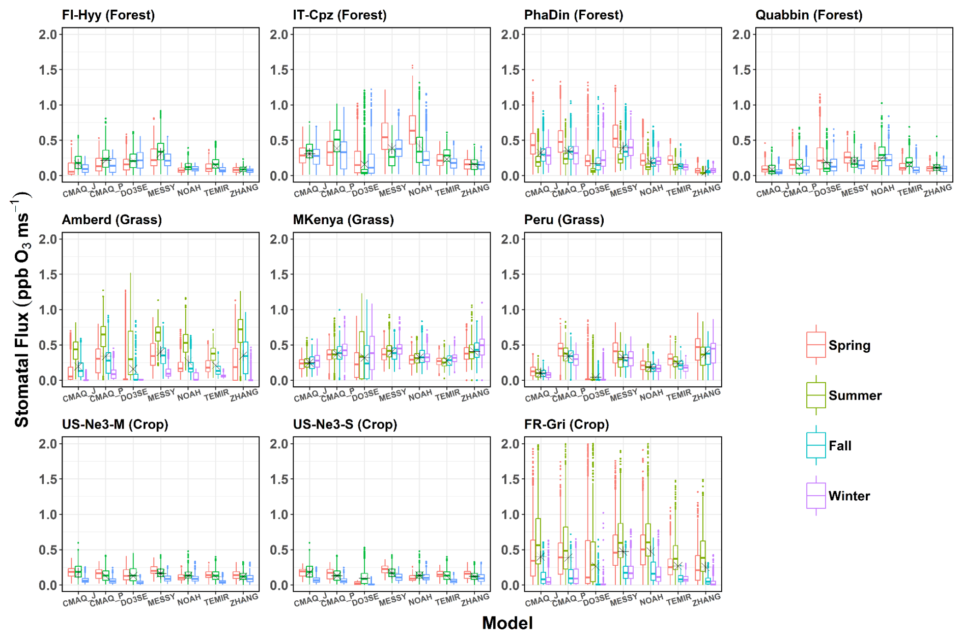
Figure 5 Box plots of seasonal mean canopy-level total stomatal O₃ flux (ppb O₃ m s⁻¹) for different models across various sites (data represent SRAD >50 W m⁻² and the growing period). Asterisks indicate the annual mean flux.

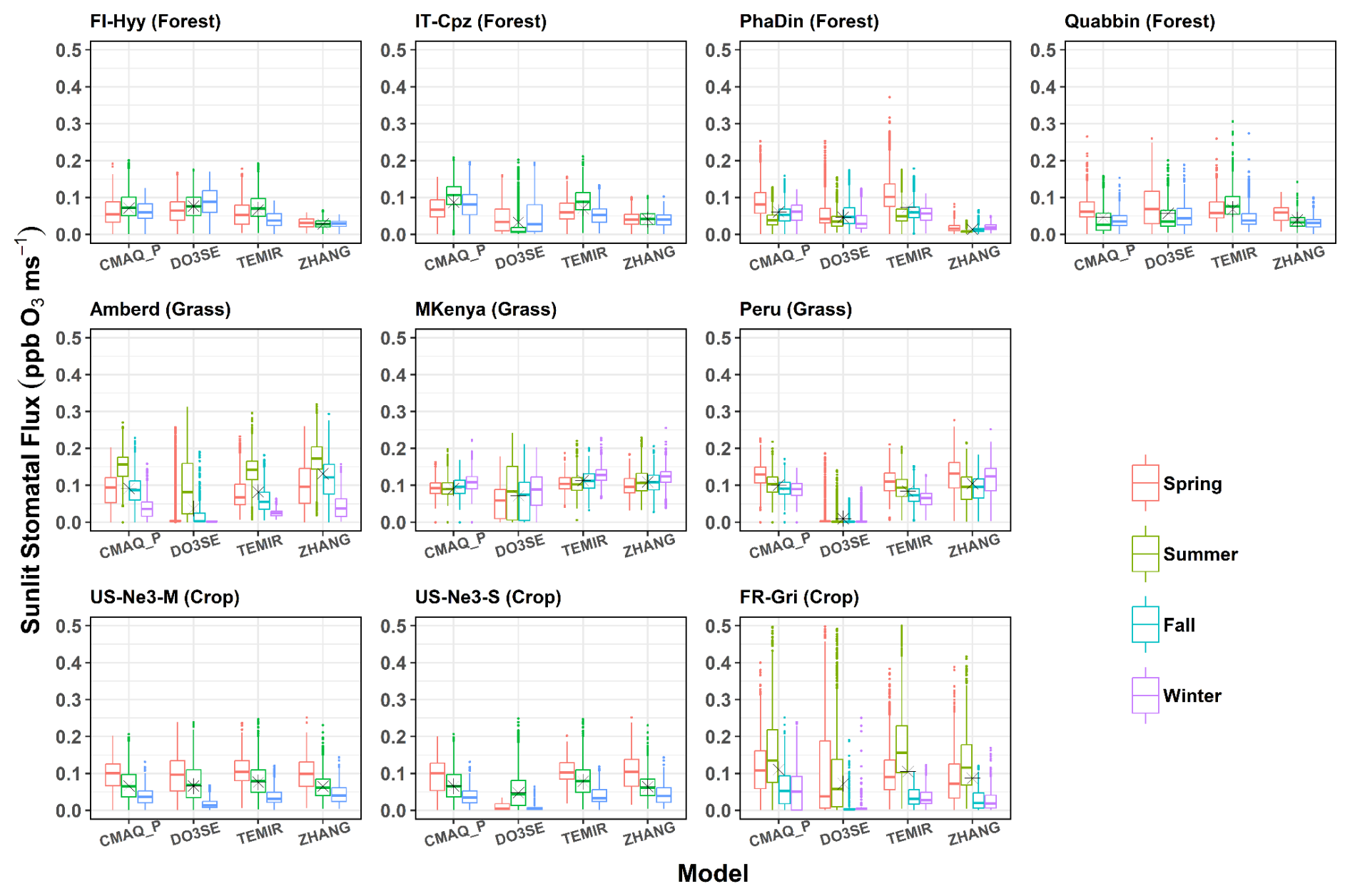
Figure 6 Box plots of seasonal mean leaf-level sunlit stomatal O₃ flux (ppb O₃ m s⁻¹) for different models across various sites (data represent SRAD >50 W m⁻² and the growing period). Asterisks indicate the annual mean flux.

3.2 Vegetation impact and variation with key input data

This section presents the POD_y calculated from the O₃ deposition by different models at nine different stations to identify trends and patterns of POD_y among land cover types and climates (Fig. 7, corresponding data in Table S9). The critical threshold for ozone damage y differs for the three land cover types. For forests and grass the y value is 1 nmol O₃ m⁻² s⁻¹ (POD₁), while O₃ damage to crops is assumed to occur only when the y threshold exceeds 6 nmol O₃ m⁻²ṡ⁻¹ (POD₆). By driving the models with changed input data of O₃, soil moisture, temperature, relative humidity, and growing season (Fig. 8) and with changed $V_{c_{\max }}/g_{\max }$ parameter (Fig. 9), we explore the sensitivity of the POD_y estimates. As shown in the previous analysis, the largest O₃ uptake and thus the highest POD_y of 28 mmol O₃ m⁻² (on average among all models) is estimated over grassland sites (compared to forest and crops) (Fig. 7). POD₁ increases linearly with time for evergreen grasslands, whereas Mt. Kenya shows the fastest accumulation (due to the highest F_st in spring and summer). Three of the four models lie in a range of 5 mmol O₃ m⁻², whereas Web-DO₃SE predicts a maximum POD_y of 10 mmol O₃ m⁻² at all grassland sites. Only at the Peru site can these low values be explained by the significantly lower G_sun and F_st,sun (compared to other models).

For forests, our modelled ensemble POD₁ median and maximum values (ranging between 8 and 25 mmol O₃ m⁻²) are similar in scale to values estimated across broad geographical regions by other studies. Karlsson et al. (2025) estimated POD₁ values across Europe with the highest values in mid-latitude Europe for coniferous (15 to 20 mmol O₃ m⁻²) and broadleaf (22 to 28 mmol O₃ m⁻²) forests. However, the ZHANG and the Web-DO₃SE model are estimated to obtain significantly lower POD₁ than CMAQ_P and TEMIR at each site. These estimates average to 16 mmol O₃ m⁻². There is no obvious pattern to which models tend to estimate higher or lower POD₁ values, but these estimates are generally consistent with G_sun (Fig. 4) and F_st,sun (Fig. 6) model estimates explained by particular model constructs or parameterizations. For instance, the ZHANG model estimates low stomatal deposition and thus also POD_y over all forests. Web-DO₃SE saw a low O₃ uptake only due to the site conditions at IT-Cpz.

For crops, the model estimates of POD₆ are a little more consistent, with modelled differences within sites only varying between ∼3 and 11 mmol O₃ m⁻²; however, this could in part be due to the overall lower POD₆ values due to the use of the higher y threshold. Median model ensemble values range between ∼7 and 12 mmol O₃ m⁻²across sites. POD₆ for staple crops has been estimated in other studies across Europe and globally. A European study (Schucht et al., 2021) on wheat found POD₆ values of up to ∼4 mmol O₃ m⁻² suggesting that our POD₆ values for the FR-Gri site tend to be too high. Feng et al. (2012) estimated maximum POD₆ values of up to 8 mmol O₃ m⁻² for winter wheat in China, though these higher values are likely driven by higher ozone concentrations. Similarly, Wang et al. (2022) also found POD₆ values for maize of up to 8 mmol O₃ m⁻². Our models give the largest range in POD₆ estimates for soybeans at the US-Ne3 site (0 to 11 mmol O₃ m⁻²). A key determinant of the range in POD_y simulated by our models, and also with estimates provided in the literature, is the value chosen for g_max (or $V_{C_{\max }}$ depending on the model construct). For example, the multiplicative g_sto models used to derive flux–response relationships (see Table 5) use g_max values of 450, 126, and 301 mmol O₃ m⁻² s⁻¹ for wheat, maize, and soybeans (UNECE LRTAP, 2017; Peng et al., 2019; Zhang et al., 2017). By contrast, our modelling uses a variety of g_max values; for example, the Web-DO₃SE model uses 450, 305, and 300 mmol O₃ m⁻² s⁻¹ for wheat, maize, and soybeans. A further consideration in parameter selection is local conditions; a study by Stella et al. (2013) found a g_max value of 296 mmol O₃ m⁻² s⁻¹ was most appropriate to describe wheat g_sto at the FR-Gri site. This variation highlights the importance of selecting appropriate model parameterization for conditions, as well as consistency of parameterization with models used to develop flux–response relationships.

Figure 7 Evolution of POD_y (mmol O₃ m⁻²) through the growing seasons at various sites.

From the sensitivity analysis, we found that all models show sensitivity of POD_y to changes in O₃, specific humidity, and temperature with varying degrees over different land cover types, possibly due to different prescribed values such as the temperature threshold (Fig. 8, corresponding absolute values in Table S10). In particular, the POD_y at all sites is most significantly changed when modifying the O₃ concentration by ±40 % (Table S11). Crop is the most sensitive land cover to O₃ changes across the different models (8.5 mmol m⁻²; 76 % POD_y change with respect to the base run), followed by forest (10.0 mmol O₃ m⁻²; 59.3 %) and grass (14.9 mmol O₃ m⁻²; 56.1 %), which is due to the plant physiognomy (Grulke and Heald, 2020). In a relative sense, the average response change in POD_y to a 40 % change in O₃ concentrations is the greatest in ZHANG (+9.2 mmol O₃ m⁻², corresponding to a 68.1 % POD_y change with respect to the base run), followed by CMAQ_P and TEMIR (12 and 11.9 mmol O₃ m⁻²; 64.8 % and 63.5 %), and then by Web-DO₃SE (11.4 mmol O₃ m⁻²; 53.0 %). Also, the POD_y estimate seems to be sensitive to humidity (Q) changes (±30 %) among all models. At forest, the POD_y estimates appear to be the most sensitive (4.6 mmol O₃ m⁻²; 27.3 %), followed by crops (2.9 mmol O₃ m⁻²; 25.9 %) and grass (4.6 mmol O₃ m⁻²; 17.3 %). The response is the greatest in TEMIR and CMAQ (between 5.7 and 6.7 mmol O₃ m⁻²; 30.7 %–35.8 %), while it is much smaller for ZHANG (usually close to zero on average). The most non-linear response was shown by Web-DO₃SE at IT-Cpz, which estimated a 5 times higher POD_y response to increasing humidity than to a humidity decrease, pointing towards the strong dryness at this site limiting factor. If temperature is changed by ±3 K the highest sensitivity was found at crops on average (2.7 mmol O₃ m⁻²; 24.1 %), followed by grass (4.6 mmol O₃ m⁻²; 17.2 %) and forest (1.6 mmol O₃ m⁻²; 9.5 %). The responses unevenly vary in sign depending on the model because the temperature change depends on the optimal temperature at the specific sites: most models estimate a POD_y decrease when increasing temperature (Fig. 5). As described in Hayes et al. (2019), a temperature increase is seen in southern countries, where temperature could limit stomatal uptake since temperature is already close to the optimum in normal conditions. From our sensitivity analysis, temperature impacts on POD_y are noticeable only for a few sites (e.g. Ambered, Mt. Kenya, and Peru) and models' response to POD_y change were different due to different thresholds used for the temperature stress factors to stomatal conductance. The greatest changes in magnitude are predicted by Web-DO₃SE (5.1 mmol O₃ m⁻²; 23.7 %), followed by CMAQ_P (3.1 mmol O₃ m⁻²; 16.7 %), ZHANG (1.9 mmol O₃ m⁻²; 14.1 %), and TEMIR (1.7 mmol O₃ m⁻²; 9.6 %). In contrast, not all models are sensitive to changes of soil water content (SWC). The greatest response is seen in CMAQ_P (−6.3 and +1.4 mmol m⁻²; −34.0 % and +7.6 %), followed by Web-DO₃SE (−2.2 and −2.2 mmol O₃ m⁻²; −10.2 % and −10.2 %) and TEMIR (−1.1 and +0.8 mmol O₃ m⁻²; −5.9 % and +4.3 %), while ZHANG shows no difference in this regard because it is not sensitive to soil moisture. The changes are largest at crops (1.5 mmol O₃ m⁻²; 13.4 %), while grass and forest show similar responses (2.8 and 1.7 mmol O₃ m⁻²; 10.5 % and 10.1 %, respectively). That is in line with De Marco et al. (2020), who show that POD_y responses to soil water changes increase with higher y threshold (here crops). The models do not appear to be sensitive to LAI 14 d shifts, with the only exception of Web-DO₃SE, which simulates a lower POD_y for both early and late LAI shifts (−2.6 mmol O₃ m⁻² on average, across all land covers). LAI is used as a proxy for growing seasons in most models, whereas Web-DO₃SE considers growing seasons directly.

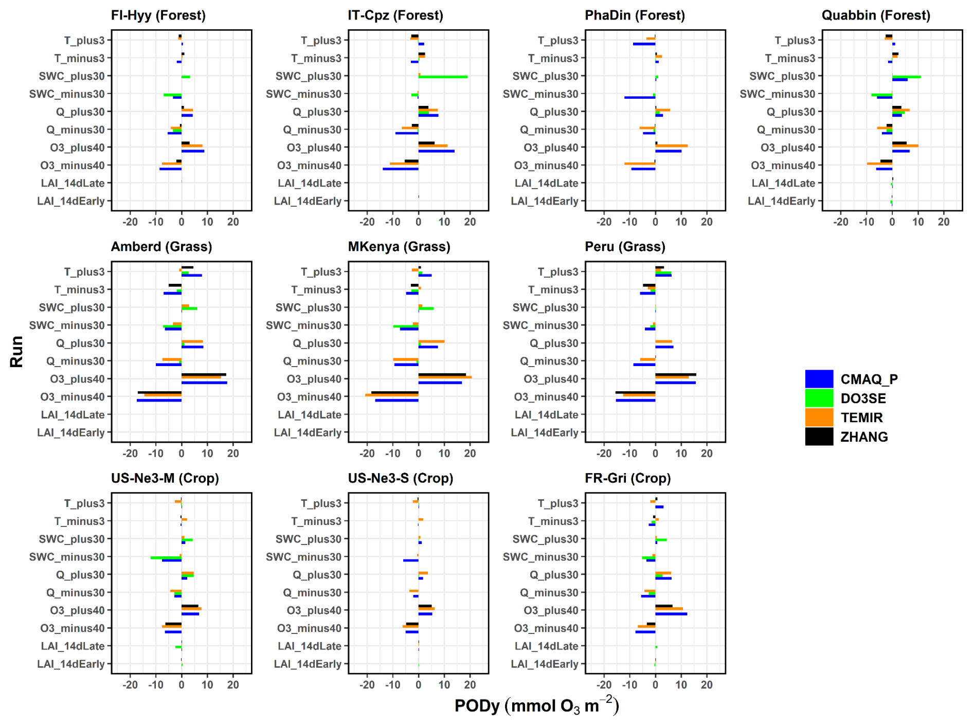
Figure 8 Meteorology sensitivity assessment: absolute change of POD_y values with respect to base run POD_y due to 10 % or 20 % variation of the temperature (T), soil water content (SWC), absolute humidity (Q), O₃, and LAI/growing season.

A 20 % change of $g_{\max }/V_{c_{\max }}$ leads to corresponding changes in POD_y values. An increase or decrease in the parameter leads to very similar changes (in ±) (Fig. 9, corresponding data in Tables S12–S14). The response appears to be generally uniform across sites. On average, the results show $+\mathrm{28.9}\pm \mathrm{22.4}$ % POD_y change for the 20 % increase in $g_{\max }/V_{c_{\max }}$ and $-\mathrm{27.4}\pm \mathrm{13.1}$ % for the 20 % decrease with the largest absolute changes in grassland (up to 8 mmol O₃ m⁻², ZHANG). At forests and crops, changes up to 5 and 3 mmol O₃ m⁻² occur, respectively. Among all sites, noticeably higher (the highest) relative changes were estimated at FR-Gri, which thus constituted the only relevant source of variability. This change is significantly different to the change at US-Ne3 (20 %–30 %) which reflects the contrasting low O₃ level at US-Ne3 compared to the highly polluted FR-Gri site. Also, the ZHANG model predicts the highest changes at crops while CMAQ_P seems insensitive. The ZHANG (and TEMIR) model appears to be the most sensitive model to the changes at most sites due to the strong dependency on the $g_{\max }/V_{c_{\max }}$ parameter (see analysis above). The only climate trend of the response is seen by the ZHANG model, which shows an average 65 % increase/decrease in wet forests (PhaDin, FI-Hyy) and only a 40 % change in dry places. Sites with very low estimates (PhaDin in ZHANG, Peru in Web-DO₃SE) were excluded from this sensitivity study.

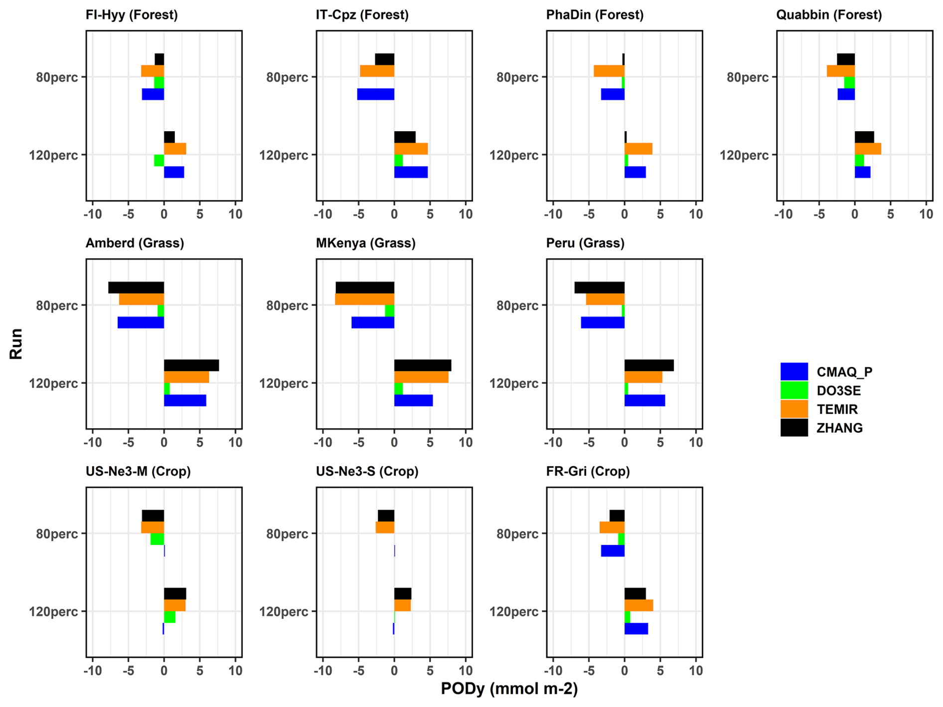
Figure 9 Land cover parameterization sensitivity assessment: absolute change of POD_y values with respect to the base run POD_y values due to 20 % variation of G_max or $V_{C_{\max }}$.

To indicate the likely damage and range of damage that our modelled values of POD_y predict, we have used POD_y flux–response relationships available in the literature that most closely represent the vegetation type and climatic location of each study site (Table 5). To estimate O₃ damage to forests we use recently derived flux–response relationships that relate POD₁ values to gross annual increment (Karlsson et al., 2025) and hence indicate the annual change in growth rate caused by O₃. The mean model ensemble estimates a percentage reduction in gross annual increment of around 5 % for FI-Hyy and Pha Din, 6 % for IT-Cpz and 14 % for Quabbin. However, the range in estimates across models is not insignificant and most extreme at the Quabbin site, with a minimum of 11 % and a maximum of 21 % around the mean 13 % value; this is due to broadleaf deciduous species being more sensitive to the O₃ dose than needleleaf species and hence more sensitive to a range of POD_y model simulations (Bücker et al., 2015). It should also be emphasized that the Pha Din site uses a European-derived flux–response relationship for an Asian forest site.

Table 5 Estimates of O₃ damage (for specific response metrics) derived from using the ensemble mean modelled POD_y values (and minimum and maximum values) with appropriate flux–response relationships based on land cover type. The climatic locations within which the flux–response relationships are derived are stated to show the relevance of their use in estimating damage. Shaded cells denote flux–response relationships that are derived outside of the broad climate region to which they are applied in this study and hence whose damage estimates should be treated with caution.

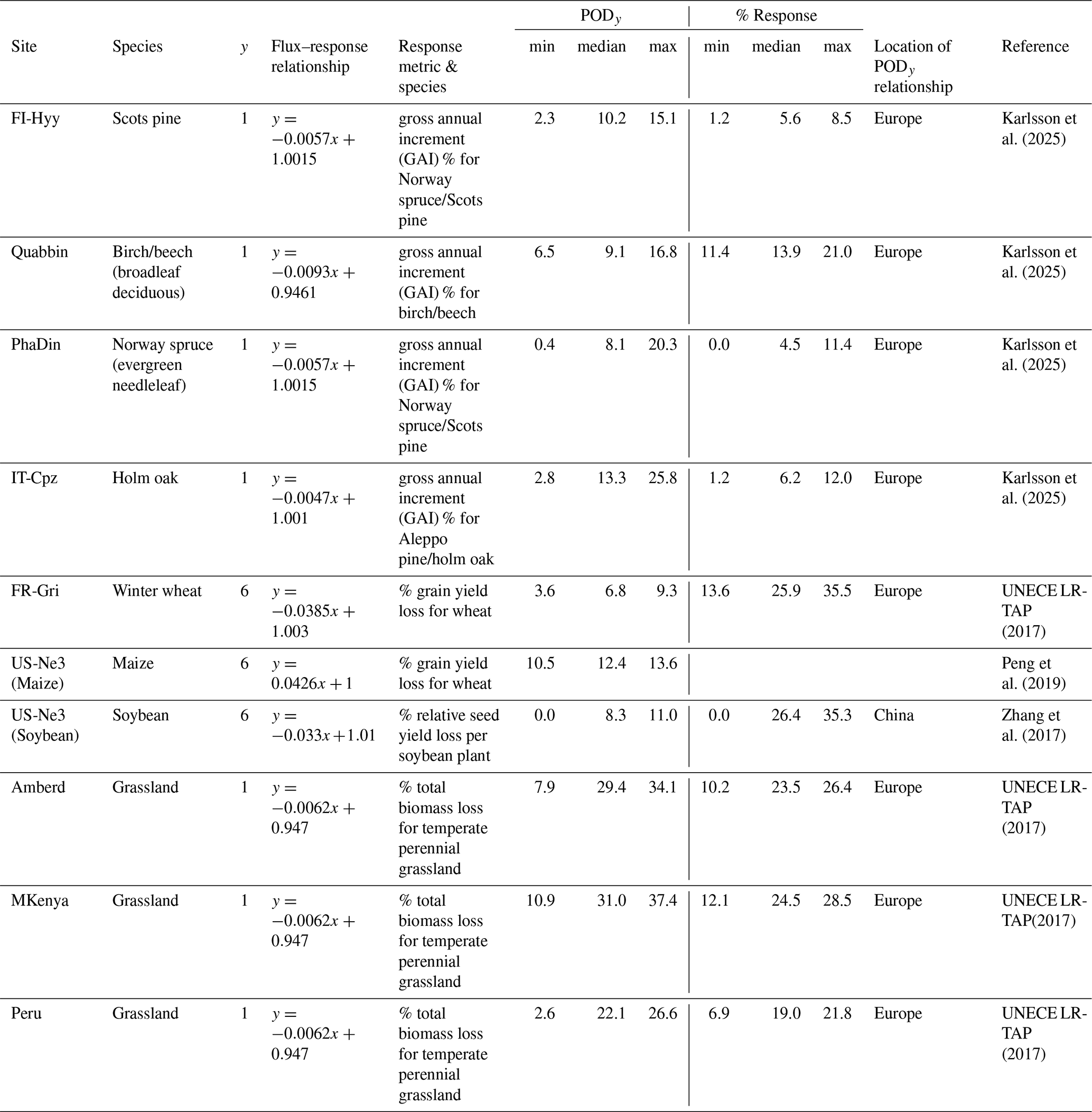
For crops, flux–response relationships are available for wheat, maize, and soybeans (UNECE LRTAP, 2917; Peng et al., 2019; Zhang et al., 2017). These relationships are derived from Europe (wheat) and China (maize and soybean). For wheat, we see a large range in percentage yield loss, with a mean model ensemble of 26 % but a maximum yield loss of 35 %. This is driven by high POD₆ values derived from CMAQ_P and TEMIR. For maize at US-Ne3 the results are very consistent, with relative grain yield loss estimates ranging from 1.4 % to 1.6 %. For soybeans at US-Ne3, the results are less consistent than maize, with a minimum and maximum of 0 % and 35 % yield around a mean of 26 %. It is important to note that a Chinese-derived flux–response relationship is used to estimate O₃ damage on both US-grown crops.

Finally, for grasslands, we estimate total biomass losses of 19 %, 24 %, and 23 % from the ensemble model mean for Peru, Mt. Kenya, and Amberd respectively. The range in model values is relatively small for Amberd and Mt. Kenya. A low minimum value of 6 % total biomass loss is estimated for Peru due to the Web-DO₃SE model having a very low POD_y at this location due to a likely oversensitive limitation to O₃ uptake caused by low temperatures.

4 Discussion and conclusion

Here we have compared six deposition schemes commonly used in atmospheric chemistry transport models. We have focussed on the stomatal component of deposition since this is acknowledged to have a substantial influence on damage to vegetation and ultimately the ability of these six models to estimate the POD_y metric designed to indicate the level of O₃ damage to forest, crops, and grasslands. The models estimate POD_y values of 28, 15, and 9 mmol O₃ m⁻² for grassland, forests, and crops, respectively. The multi-model mean estimates are generally in the expected range, which suggests that the stomatal flux output of these models could be used for O₃ impact assessments. We also explored the differences in POD_y by geographical location. When comparing one vegetation type, we find multiple drivers including O₃ concentration. The different model types are not the driving force; instead, the models can predict similar results.

There are three key reasons for differences in dry deposition model estimates: (i) model construct and the inclusion/exclusion of important factors that determine G_st and G_sun; (ii) model parameterization, which may characterize the land cover types; and (iii) differing model sensitivity to climate variables (seasonal, location effects) in estimates of stomatal deposition. The model comparison of stomatal conductance and stomatal dry deposition for ozone helps us to understand the differences between models. We found that models simulate generally reasonable stomatal deposition of 0.5–0.8 cm s⁻¹ in summer, whereas the different model types often agree very well with each other. The stomatal conductance estimates among the models agree with correlation coefficients of 0.75, 0.80, and 0.85 for forests, crops, and grasslands. Thereby, the nine sites selected for this study also reflect different climate conditions; however the selection of sites that provide such broad representations also means that the analysis and the results cannot be generalized. The global coverage, diverse land types, and varying meteorological conditions of the nine sites resulted in widespread model responses to soil moisture (Fig. 8) while appearing to be insensitive to changes of LAI (Fig. 9). The former underscored the idiosyncratic features and hence potential limitations of individual models, whereas the latter gave us confidence in model capabilities despite the different constructs and parameterizations of the models. The model differences, identified during this analysis, can be explained by the model's dependence on the meteorological conditions at sites. Indeed, both model structure (e.g. Raghav et al., 2023) and parameters (Fares et al., 2013) can affect the accuracy of stomatal conductance models. However, studies have shown that when properly calibrated against field observations, structurally different stomatal models can produce similar stomatal conductance (Fares et al., 2013; Mäkelä et al., 2019). Calibrating the key parameters of stomatal conductance models (e.g. $g_{\max }/V_{c_{\max }}$) is a crucial next step to improve the accuracy of stomatal conductance and POD_y estimates, as our sensitivity tests show a direct and possible non-linear relationship between POD_y and $g_{\max }/V_{c_{\max }}$ (e.g. at FR-Gri). This is possible with the recent availability of standardized global eddy flux (FLUXNET, Pastorello et al., 2020) and sap flow (SAPFLUXNET, Poyatos et al., 2021) data.

To estimate POD_y for a representative leaf of the upper canopy, the sunlit leaf must be distinguished from the total leaf. Since the effects-based community recognized that sunlit leaves contribute most to carbon assimilation throughout the growing season or O₃-sensitive period (e.g. in wheat, this is considered to be the time from anthesis to maturity), it will better represent damaging O₃ uptake. All flux–response relationships for POD_y are developed for such a representative leaf. This is an important distinction since previous model comparison studies (e.g. Clifton et al., 2023) have tended to focus on whole canopy dynamics. These are important to estimate accurately, but estimating POD_y requires additional canopy-level processes, which need (i) O₃ concentration at the top of the canopy, (ii) wind speed at the top of the canopy, and (iii) G_sun of a representative leaf at the top of the canopy. Studies (Emberson, 2020, and references therein) have established thresholds for different land cover types, which are used to provide y values for the selected sites with specific land cover types in this study. Some studies suggest that the y threshold for land cover types may vary by global region (e.g. a number of studies suggest higher y values of up to 12 nmol O₃ m² s⁻¹ are more appropriate for crops and forest tree species in Asia). In this study, which focuses on comparing across models, we maintain consistency and use common y threshold values for each land cover type. However, this is an aspect that would benefit from further study in the future since estimating POD_y values with higher thresholds is more challenging for all types of model given the less frequent occurrences of such high O₃ doses.

Our models estimate 30 %–50 % of stomatal O₃ deposition at sunlit leaves. Thereby, the model estimates of the total stomatal flux are more widespread (during one season) than the estimates of the sunlit only, which suggests an important role of the model's partitioning in two big leaves. When calculating POD_y model means, estimates generally agree with the literature, but most discrepancies between model estimates of POD_y ultimately come down to the differences in simulations of stomatal conductance. The sensitivity analysis of POD_y yields ozone as the most important input variable, to whose changes all models respond similarly. Considering all models and sites together, POD_y was affected most by the O₃ concentration (±60 %–80 % site-dependent; i.e. higher O₃ concentration leads to higher POD_y), followed by humidity (30 %–50 % site-dependent impact). Soil moisture impacts were also significant for the CMAQ_P and Web-DO₃SE model (up to ±68 % and 22 % change). The sensitivity to temperature changes varies strongly among the model and its parameterization. As the plant canopy acts as a persistent sink of O₃, there is a significant vertical gradient of O₃ within the atmospheric surface layer. For example, Travis and Jacob (2019) show that the midday O₃ concentration at 65 m above ground (mid-point of a first vertical layer of GEOS-Chem v9-02) is 3 ppb higher than the O₃ concentration at 10 m above ground (inferred by Monin–Obukhov similarity theory, MOST) over the Southeastern United States. A mismatch between O₃ measurement height and canopy height can lead to inaccurate POD_y calculation (Gerosa et al., 2017). An O₃ bias of 2 ppb as estimated by, for example, Tarasick et al. (2019) would lead to a change of 6 %–7 % in POD1 (Gerosa et al., 2017). Similarly, we show that the errors in O₃ concentrations propagate non-linearly to POD_y (i.e. 40 % changes in O₃ leads to 53 %–68 % changes in POD_y); such a mismatch should be carefully avoided by applying atmospheric surface layer theories (e.g. MOST) to estimate the vertical profile of O₃, and therefore the canopy-top O₃ concentration, if direct measurement or model output of O₃ at canopy top is not available.

Finally, we use flux–response relationships for temperate deciduous (beech/birch), temperate needleleaf (Norway spruce (Picea abies)), crops (wheat (Triticum aestivum), maize (Zea mays), soybeans (Glycine max)), and grassland (Lolium perenne) to suggest the potential likely variation of damage estimates by land cover type and climatic region. These relationships have predominantly been developed for European and Asia forest and crop species. Therefore, they should be applied to other climate regions with caution, although recent evidence suggests that tropical forest species may have similar sensitivity to O₃ as European species (Cheeseman et al., 2024). Although there is rather large variability in POD_y values estimated by the model, the median values are relatively robust. Unfortunately, there is only statistical or modelled evidence of actual O₃ damage and only at a few of the sites investigated. Modelled evidence uses stomatal ozone flux models similar to those used in this study but which have been parameterized for local site conditions (Stella et al., 2013, for FR-Gri wheat). Simulations with a terrestrial biosphere model suggested an average long-term O₃ inhibition of 10.4 % for the period 1992–2011 at the Harvard site (Yue et al., 2016); this compares to our model ensemble estimate of 14 % GAI biomass loss for Quabbin. A significant but small NEP reduction was found during spring in the Italian Castelporziano forest site (up to −1.37 %) but not at the FI-Hyy or FR-Gri sites (Savi et al., 2020). Our modelling estimated substantially lower POD_y values and associated damage at Hyy and IT-Cpz than Quabbin, though we would expect to see a more substantial O₃ effect than that demonstrated by the NEP statistical modelling (i.e. 5 % and 6 % GAI biomass loss at FI-Hyy and IT-Cpz respectively). Similar simulations with a different terrestrial biosphere model found only moderate O₃ damage effects (GPP reductions of 4 %–6 %; Yue and Unger, 2014). This result is driven by low ambient ozone concentrations but also by the choice of a C₄ photosynthetic mechanism to estimate stomatal conductance which gives relatively high water use efficiency). These simulations also suggested that the US-Ne3 experienced a higher ozone effect on GPP than Harvard, which is consistent with our modelling for soybeans (but not maize, generally considered an O₃-tolerant crop species; Mills et al., 2011). According to the POD₆ estimates made using a SURFATM model, parameterized for Grignon wheat, POD₆ values of 1.094 mmol O₃ m⁻² were estimated from 1 April to 1 July 2009, which compared with our range of 3.6 to 9.3; the locally parameterized values gave estimated crop yield losses of 4.2 %, compared to our median model ensemble estimates of 25 % for the winter wheat. This is most likely due to the lower g_max value used in the local parameterization (296 mmol O₃ m⁻² s⁻¹). However, no recording of actual damage is given at the FR-Gri site, so it is not possible to tell which of these simulated damage estimates is closer to reality.

The experiments performed here with varying climate and vegetation input data also find a similar sensitivity of POD_y to O₃. It is helpful to have a range of models and model constructs in deposition schemes, especially where these have been developed for particular land cover types. When used in damage estimates it is important to ensure that key stressors are included, which may be important for that respective geographical region (such as soil and vapour pressure deficit). Recognizing that several deposition schemes would be able to reliably predict POD_y for different climates and cover types once they have been parameterized appropriately will extend the usefulness of flux–response relationships.

Overall, this study has demonstrated the widespread applicability and consensus among various numerical stomatal flux methods. Both semi-mechanistic and empirical models can generally represent observed ozone fluxes among different land cover types and climates. We identified the key model constructs and parameterizations that cause differences in POD_y estimates. However, none of the models clearly shows a superior overall performance. Instead, all models can be effectively applied, each with its own strengths and weaknesses. Our findings present exciting opportunities to extend applications beyond specific sites and growing seasons, enabling comprehensive global stomatal flux studies over longer periods. Integrating the TOAR database with the Web-DO₃SE model enables automatic model runs for ozone–vegetation impact assessment at a large range of sites using the TOAR database.

Appendix A: Abbreviations

rsmin	Minimum stomatal resistance [s m−1]
gsmax	Maximum stomatal conductance [m s−1]
RH	Relative humidity [%]
LAI	Leaf area index [m2 m−2]
sd, sn	Snow depth [m] and snow cover
ssrd, strd	Solar and thermal flux at surface [W m−2]
sw	Soil wetness [m]
al_vis:	Albedo (visible)
cwv	Canopy water content [kg m−2]
SWC	Soil water content
SM	Soil moisture [m3 m−3]
wdir	Wind direction [°]
wspeed	Wind speed [m s−1]
cv	Vegetation fraction [m2 m−2]
P	Precipitation [mm]
P_rate	Precipitation rate [mm h−1], [kg m−2 s−1], [m s−1]
Tair, Tsoil, T2m	Air, soil, 2 m temperature in [K]
VPD	Vapour pressure deficit [kPa]
Pa	Air pressure [hPa]
Rn, Gr	Net and global radiation [W m−2]
u*	Friction velocity [m s−1]
O3, CO2	O3 and CO2 concentration [ppb], [ppt]
h_dis, z0	Displacement height [m], roughness length [m]
CF	Cloud fraction
LUC	Land use category