From small-scale variability to mesoscale stability in surface ocean pH: implications for air–sea CO₂ equilibration

One important aspect of understanding ocean acidification is the nature and drivers of pH variability in surface waters on smaller spatial (i.e. areas up to 100 km²) and temporal (i.e. days) scales. However, there has been a lack of high-quality pH data at sufficiently high resolution. Here, we describe a simple optical system for continuous high-resolution surface seawater pH measurements. The system includes a PyroScience pH optode placed in a flow-through cell directly connected to the underway supply of a ship through which near-surface seawater is constantly pumped. Seawater pH is measured at a rate of 2 to 4 measurements min⁻¹ and is cross-calibrated using discrete carbonate system observations (total alkalinity, dissolved inorganic carbon, and nutrients). This setup was used during two research cruises in different oceanographic conditions: the North Atlantic Ocean (December 2020–January 2021) and the South Pacific Ocean (February–April 2022). By leveraging this novel high-frequency measurement approach, our findings reveal fine-scale fluctuations in surface seawater pH across the North Atlantic and South Pacific oceans. While temperature is a significant abiotic factor driving these variations, it does not account for all observed changes. Instead, our results highlight the interplay between temperature, biological activity, and waters with distinct temperature–salinity properties and their impact on pH. Notably, the variability differed between the two regions, suggesting differences in the dominant factors influencing pH. In the South Pacific, biological processes appeared to be mostly responsible for pH variability, while in the North Atlantic, additional abiotic and biotic factors complicated the correlation between expected and observed pH changes. While our findings indicate that broader ocean-basin-scale analyses based on lower-resolution datasets can effectively capture surface ocean CO₂ variability at a global scale, they also highlight the necessity of fine-scale observations for resolving regional processes and their drivers, which is essential for improving predictive models of ocean acidification and air–sea CO₂ exchange.

1 Introduction

Ocean chemistry is changing due to the uptake of anthropogenic CO₂ from the atmosphere (DeVries, 2022). The uptake of atmospheric CO₂ by the ocean's surface increases hydrogen ion concentration, a process known as ocean acidification, which has led to a 30 %–40 % rise in hydrogen ion concentration (i.e. surface seawater acidity) and a corresponding pH decrease of ∼0.1 since around 1850 (Gattuso et al., 2015; Jiang et al., 2019; Orr et al., 2005). These changes have already significantly impacted marine organisms, especially marine calcifiers (Doney et al., 2020; Gattuso et al., 2015; Osborne et al., 2020), and pH is projected to decline by ∼0.3 by 2100 (Figuerola et al., 2021).

High-resolution studies of surface ocean carbonate chemistry and air–sea CO₂ exchange have significantly advanced our understanding of the upper ocean's carbon cycle. However, gaps remain, particularly at fine spatio-temporal scales (e.g. variability over hours and a few kilometres). At these scales, changes in pH over short time periods can be an important control on the ocean's buffering capacity and response to CO₂ uptake, highlighting the need for further detailed observations (Cornwall et al., 2013; Egilsdottir et al., 2013; James et al., 2020; Qu et al., 2017; Wei et al., 2022).

Advancements in the last decade and a half have enhanced the capacity for accurate and precise in situ pH measurements. For example, Martz et al. (2010) developed an autonomous sensor tailored for continuous deployment in marine environments that allows the recording of high-resolution pH fluctuations. Autonomous surface vehicles in coastal upwelling systems have also been used to capture the intricate partial pressure of CO₂ (pCO₂) and pH dynamics, even in complex environments where rapid biogeochemical changes occur due to natural phenomena like upwelling (Chavez et al., 2018; Cryer et al., 2020; Possenti et al., 2021). Staudinger et al. (2018) also developed an optode system capable of simultaneously measuring oxygen, carbon dioxide, and pH in seawater. This system was designed for extended deployment (i.e. days) in marine environments, enabling continuous monitoring (with measurement intervals between 1 s and 1 h) of these parameters. Additionally, Sutton et al. (2019) detailed the implementation of autonomous seawater pCO₂ and pH time series from 40 surface buoys, broadening the scope of observations at fixed time series sites. Staudinger et al. (2019) introduced fast and stable optical pH sensor materials specifically for oceanographic applications, enhancing the ability to measure pH under various environmental conditions.

These technological advancements have facilitated significant scientific progress. Field measurements conducted using submersible spectrophotometric sensors have revealed fine-scale variations in pH in coastal waters and shed light on localised acidification processes (Cornwall et al., 2013). The implementation of autonomous seawater pCO₂ and pH time series as described by Sutton et al. (2019) has enhanced our ability to characterise sub-seasonal variability in the ocean. These efforts represent important progress that can be built upon to further understand fine-scale ocean dynamics.

Fine-spatio-temporal-scale variability in surface ocean pH is hard to capture because it is driven by a complex interplay of processes, including physical mixing, biological activity (i.e. photosynthesis and respiration), thermal variability, and air–sea CO₂ fluxes (Faassen et al., 2023; Hofmann et al., 2011; Price et al., 2012). Physical mixing moderates surface oceanic pH by redistributing dissolved CO₂, nutrients, and heat throughout the water column. Mixing also mitigates extreme pH fluctuations by diluting surface concentrations of CO₂ during periods of high biological activity or temperature-induced CO₂ release (Egea et al., 2018; Li et al., 2019). Photosynthetic activity can decrease CO₂, leading to an increase in pH during daylight hours, while respiration dominates at night, releasing CO₂ and lowering pH (Fujii et al., 2021; Jokiel et al., 2014). Warmer waters decrease CO₂ solubility and increase pH, while cooler waters increase solubility, promoting CO₂ uptake and decreasing pH, although the timescales of these processes differ, with some changes occurring instantaneously and others after equilibration (Zeebe and Wolf-Gladrow, 2001). Instantaneous changes are driven by physical and chemical reactions, while equilibration processes involve longer-term adjustments such as air–sea gas exchange and the mixing of surface waters with deeper layers (Emerson and Hedges, 2008). When atmospheric CO₂ exceeds oceanic CO₂, the ocean takes up CO₂, lowering pH; conversely, when atmospheric CO₂ decreases below oceanic CO₂, outgassing occurs, raising pH (Caldeira and Wickett, 2005; Orr et al., 2005). Although each of these processes has its distinct impact on pH, their combined effects regulate the ocean's carbon cycle and its interaction with the atmosphere.

Recent studies on air–sea CO₂ equilibration timescales have highlighted significant regional variations, particularly between the North Atlantic and South Pacific oceans (Jones et al., 2014). In the North Atlantic, equilibration timescales for CO₂ between the atmosphere and the ocean's surface mixed layer vary significantly with latitude. In regions above 55° N, these timescales can extend up to 18 months, while at lower latitudes, such as around 30° N, they range from 3 to 6 months (Jones et al., 2014). These long equilibration timescales reduce the extent to which the ocean can buffer short-term changes in surface pH. On pentadal and longer timescales, the air–sea CO₂ flux in the North Atlantic is driven primarily by changes in ΔpCO₂, while gas transfer velocity plays a more significant role only on interannual and shorter timescales (Couldrey et al., 2016).

Cooler temperatures at higher latitudes increase CO₂ solubility, resulting in higher dissolved inorganic carbon (DIC), and upwelling brings DIC- and total alkalinity (TA)-rich deep waters to the surface (Wu et al., 2019). These factors further increase the amount of CO₂ that needs to be exchanged with the atmosphere, further prolonging equilibration times. The South Pacific, with its shallower mixed layers and higher average surface temperatures, facilitates shorter equilibration times and enhances CO₂ uptake rates (i.e. 3 to 4 months; Jones et al., 2014). Wu et al. (2019) also showed that high biological productivity in these areas significantly impacts DIC, potentially reducing surface DIC more quickly.

Here, we test a high-frequency optical system to investigate how surface seawater pH varies across fine spatio-temporal scales, focusing on changes occurring over areas of up to 100 km² and timescales of hours to days across different ocean basins (i.e. North Atlantic and South Pacific oceans) and identify abiotic and biotic factors driving these variations. We use direct, high-frequency measurements of surface seawater pH and estimate TA to resolve the rest of the carbonate system. This novel setup provides new insights into processes, such as temperature, hydrodynamic mixing, and biological activity, that influence fine-scale spatio-temporal variability in pH.

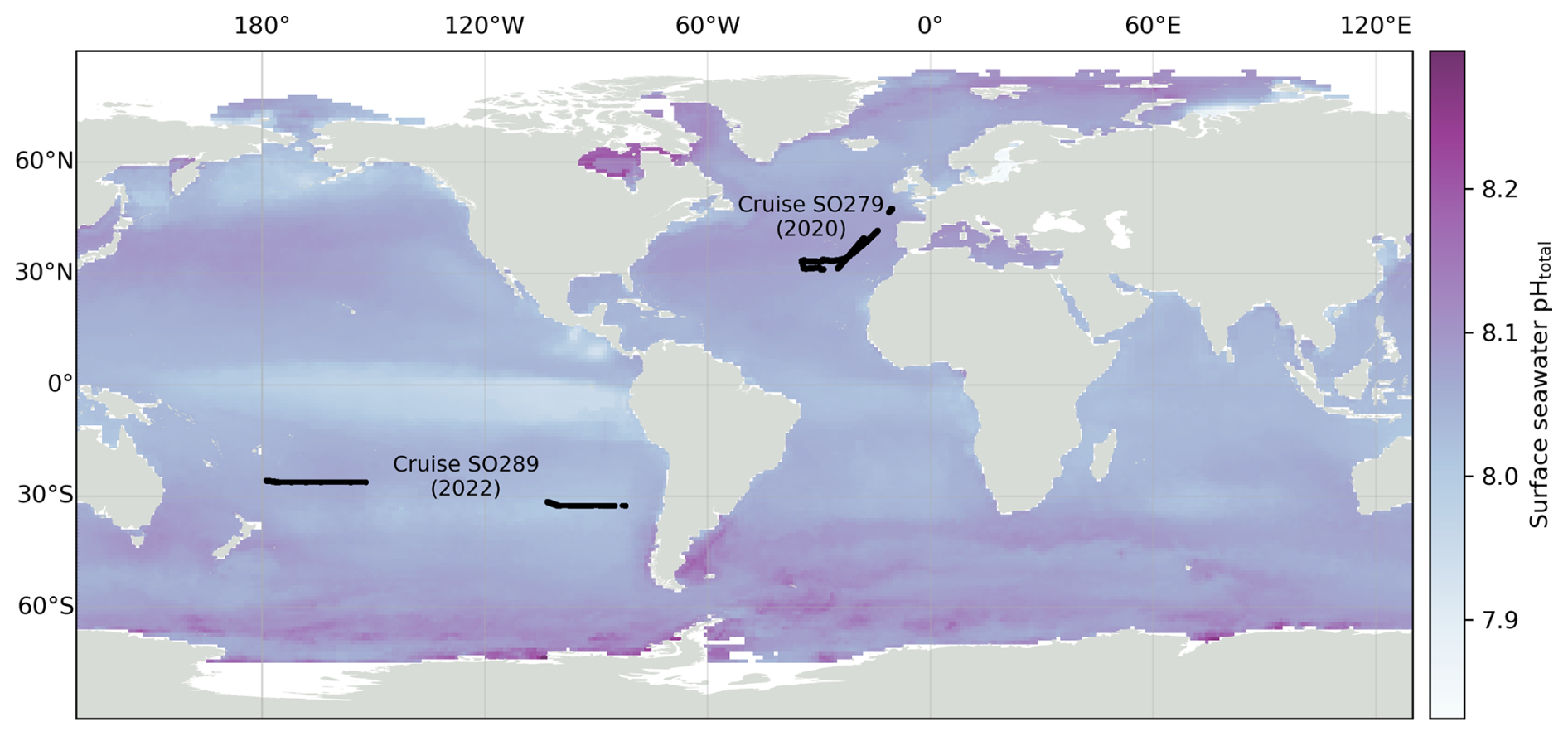
Figure 1 Locations of pH measurements during the two oceanographic cruises used in this study: SO279 in the North Atlantic (December 2020 to January 2021) and SO289 in the South Pacific (February–April 2022). Surface seawater pH on the total scale from Gregor and Gruber (2021) for December 2022 from the OceanSODA product is shown in the background.

2 Materials and procedures

2.1 Study areas

Two datasets from separate oceanic regions were used: research expeditions SO279 in the North Atlantic Ocean and SO289 in the South Pacific Ocean, both on the German R/V Sonne (Fig. 1).

Expedition SO279 in January to December 2020, conducted in the Azores region of the North Atlantic Ocean (Fig. 1), was part of the NAPTRAM research programme investigating the transport pathways of plastic and microplastic debris (Beck et al., 2021). The data collection included discrete samples from a CTD rosette (n=77; Delaigue et al., 2021a), with measurements of DIC, TA, and nutrients (silicate, phosphate ammonium, nitrite, and nitrate + nitrite); discrete samples from the underway water system (UWS; n=51; Delaigue et al., 2021c) also measuring these parameters; and a high-resolution UWS time series of ocean surface pH (over 43 000 data points; Delaigue et al., 2021b).

The South Pacific GEOTRACES cruise SO289, from Valparaiso (Chile) to Noumea (New Caledonia) under the GEOTRACES GP21 initiative, was conducted from February to April 2022 (Fig. 1; Achterberg et al., 2022). The data collection also included the same parameters as SO279, with discrete samples from a CTD rosette (n=395; Delaigue et al., 2023c), discrete samples from the UWS (n=32; Delaigue et al., 2023b), and another high-resolution UWS time series of ocean surface pH from the optode system (over 78 000 data points; Delaigue et al., 2023a).

2.2 Integrated shipboard optode system for continuous pH measurements

We used a pH optode (PHROBSC-PK8T, for pH range 7.0–9.0 on the total scale; PyroScience GmbH), made of a robust cap adapter fibre with a stainless-steel tip (length = 10 cm, diameter = 4 mm) and disposable plastic screw cap with an integrated pH sensor. The total scale accounts for sulfate ion dissociation in seawater, providing a more accurate representation of carbonate system equilibria compared to other pH scales commonly used in marine chemistry. Unless explicitly stated otherwise, all references to pH in this paper refer to pH on the total scale. The manufacturer-reported accuracy of the optode is ±0.05 for pH 7.5–9.0 and ±0.1 for pH 7.0–7.5 after a two-point calibration, with a precision of ±0.003 at pH 8.0.

The optode was connected to a meter combined with a pressure-stable optical connector (optical feed-through; OEM module Pico-pH-SUB; PyroScience GmbH; Fig. 2). Briefly, the optical pH sensor is constructed using the PyroScience REDFLASH technology, which uses a pH neutral reference indicator and a pH-responsive luminescent dye. These elements are activated using a specifically tuned orange-red light with a wavelength ranging between 610–630 nm, which triggers a bright luminescence emission in the near-infrared (NIR) band, spanning 760–790 nm. At elevated pH, the fluorescence from the pH marker is diminished, leaving only the NIR emission of the reference indicator noticeable. As the acidity increases, the pH marker is protonated, which results in a heightened NIR luminescence that is detected along with the emissions of both indicators. The measurement approach uses red excitation light modulated in a sinusoidal manner, leading to a similar modulation of the NIR emission, albeit with a phase discrepancy. This phase variation is registered by the PyroScience OEM module and subsequently converted into a total pH measurement.

Automatic temperature compensation of the optical pH sensor was achieved using a flexible Teflon-coated temperature probe (Pt100 Temperature Probe, PyroScience GmbH; Fig. 2) soldered onto the OEM module. The optode was placed in a closed flow-through cell directly connected to the underway supply of the ship through which seawater was pumped at a constant rate (6 L min⁻¹ for SO279 and 9 L min⁻¹ for SO289; 2.5 m depth) and stirred using a magnetic stirrer (Fig. 2). The entire setup was kept inside a closed box to isolate the optical instrument from any other light source (Fig. 2). All seawater first went through a thermo-salinograph close to the water source, which also measured salinity, temperature, and chlorophyll a fluorescence (chl a), before going through the pH setup (Fig. 2).

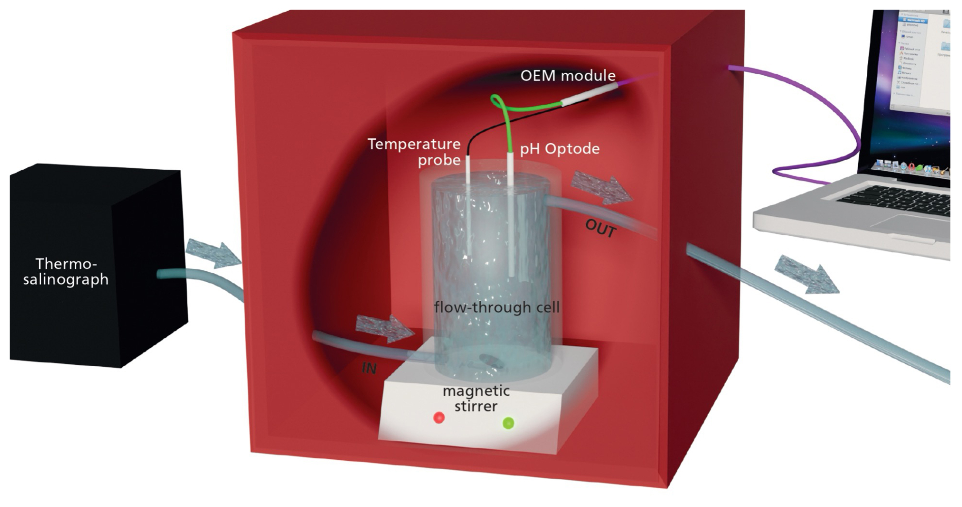
Figure 2 Schematic representation of the optical continuous pH measurement system. Arrows indicate the direction of flow-through tubing. The system consists of the following components: a thermo-salinograph; a flow-through cell, a magnetic stirrer, a fibre-based pH optode, a flexible Teflon-coated temperature probe, a fibre-optic meter OEM module Pico-pH-SUB, and a portable computer. All elements inside the red box are in the dark to avoid any light disturbance.

2.3 Initial calibration and underway measurements

Direct measurements of surface water (∼3 m depth) pH were carried out at a frequency of 2 measurements min⁻¹ for the North Atlantic cruise and 4 measurements min⁻¹ for the South Pacific cruise.

A one-point calibration of the temperature probe was performed against a thermometer inside a water bath (Lauda Ecoline RE106). A two-point calibration of the pH sensor was conducted following the manufacturer's recommended procedure, using PyroScience pH buffer capsules (pH 2 or pH 4 for the acidic calibration point, pH 10 or pH 11 for the basic calibration points). These calibration points deliberately fall far outside the sensor's operating range from pH 7–9 to characterise its maximum and minimum responses. Buffers were prepared by dissolving each capsule's powder into 100 mL of Milli-Q water.

To further refine the accuracy of the measurements, a pH offset adjustment was applied using certified reference material (CRM, batches #189, #195, and #198; provided by Andrew Dickson, Scripps Institution of Oceanography). Although CRMs do not provide direct certified pH values, we calculated pH_CRM from the CRM TA and DIC using the carbonate system equilibrium constants from Lueker et al. (2000). This pH_CRM value was then used to adjust the optode-based pH measurements to improve accuracy and align them with discrete observations.

To assess the robustness of the pH optode, resolution surface measurements of the partial pressure of CO₂ (pCO₂) and pH (samipH) were added as points of comparison. The pH optode, pCO₂ sensor, and samipH sensor were all installed on the same surface seawater supply, which was continuously pumped from approximately 2.5 m depth into the sink of the underway laboratory during the cruise. The PyroScience pH sensor received water from a split of this same supply, ensuring all sensors were sampling the same source water.

Surface pCO₂ was measured using a factory-calibrated commercial sensor (HydroC, 4H-JENA Engineering GmbH, Germany; Fietzek et al., 2014) at a 1 min sampling interval. An automatic zero-point calibration was performed every 6 h to correct for sensor drift. The recorded pCO₂ values were subsequently adjusted following Takahashi et al. (2006) to reflect in situ sea surface temperature.

Surface pH, reported on the total scale, was measured using a factory-calibrated sensor (Sunburst Sensors, USA) at 15 min intervals. The pH data were calibrated using sea surface salinity and temperature according to the equations provided by Liu et al. (2011) and Millero (2007), respectively.

2.4 Discrete sampling and analysis for other CO₂ parameters

The underway seawater system was subsampled from the cell every 12 h via silicone tubing for TA and DIC following an internationally established protocol (Dickson et al., 2007). TA was sampled in Azlon™ HDPE wide-neck round 150 mL bottles filled to the neck and poisoned with 50 µL saturated HgCl₂. DIC was sampled into Labco Exetainer^® 12 mL borosilicate vials and poisoned with 15 µL saturated HgCl₂. Samples were stored at 4 °C whenever possible and kept in the dark until analysis.

All TA and DIC analysis was carried out at the Royal Netherlands Institute for Sea Research, Texel (NIOZ). The analysis was calibrated using certified reference material (CRM, batches #189, #195, and #198; provided by Andrew Dickson, Scripps Institution of Oceanography). TA was determined using a Versatile INstrument for the Determination of Total inorganic carbon and titration Alkalinity (VINDTA 3C #017 and #014, Marianda, Germany). The instrument performed an open-cell, potentiometric titration of a seawater subsample with 0.1 M hydrochloric acid (HCl). Results were then recalculated using a modified least-squares fitting as implemented by Calkulate v3.1.0 (Humphreys and Matthews, 2020). DIC concentrations were determined using either the VINDTA system (SO279 samples and part of SO289 samples) or the QuAAtro Gas Segmented Continuous Flow Analyzer (CFA, SEAL Analytical; SO289 samples). Briefly, the VINDTA measures DIC by acidifying a seawater sample, which releases CO₂ that is then quantified through a coulometric titration cell. Similarly, the QuAAtro CFA uses acidification to liberate CO₂, which then discolours a slightly alkaline phenolphthalein pink coloured solution which is measured spectrophotometrically at 520 nm (Stoll et al., 2001).

For cruise SO279, nutrient samples were gathered using 60 mL syringes made of high-density polyethylene, which were connected to a three-way valve by tubing, drawing directly from the CTD-rosette bottles to avoid air exposure. Immediately upon collection, the samples were taken to the laboratory for processing, where they were filtered through a dual-layer filter with pore sizes of 0.8 and 0.2 µm. All samples were stored at −20 °C in a freezer except Si, samples of which were stored at 4 °C in a cold room until analysis back at NIOZ. Nutrients were analysed using a QuAAtro Continuous Flow Analyser. Measurements were made simultaneously for Si, PO₄, NH₄, NO₃, and NO₂. All measurements were calibrated with standards diluted in low-nutrient seawater (LNSW) in the salinity range of the stations (approx. 34–37) to ensure that analysis remained within the same ionic strength. Prior to analysis, all samples were brought to laboratory temperature in about 1 to 2 h. To avoid gas exchange and evaporation during the runs with NH₄ analysis, all vials including the calibration standards were covered with Parafilm under tension before being placed into the autosampler so that the sharpened sample needle easily penetrated through the film, leaving only a small hole. Silicate samples were measured separately on a TRAACS Gas Segmented Continuous Flow Analyser (manufactured by Bran + Lubbe, now SEAL Analytical) following Strickland and Parsons (1972). A sampler rate of 60 samples per hour was also used for all analyses. Calibration standards were diluted from stock solutions of the different nutrients in 0.2 µm filtered LNSW diluted with de-ionised water to obtain approximately the same salinity as the samples and were freshly prepared every day. This diluted LNSW was also used as the baseline water for the analysis and in between the samples. Each run of the system had a correlation coefficient of at least 0.9999 for 10 calibration points. The samples were measured from the lowest to the highest concentration, i.e. from the surface to deep waters in order to reduce carry-over effects. Concentrations were recorded in µM at an average container temperature of 23.0 °C and later converted to µmol kg⁻¹ by dividing the recorded concentration by the sample density, calculated following Millero and Poisson (1981).

For cruise SO289, nutrient analysis was carried out on seawater from every Niskin bottle triggered at various depths during each cast. The seawater was transferred into 15 mL polypropylene vials. Each container and its cap were rinsed three times with seawater before filling. If immediate analysis was not possible, samples were stored in a fridge at 4 °C in the dark. Macronutrients were analysed on board using a segmented flow injection analysis with a Seal Analytical QUAATRO39 auto-analyser that includes an XY2 autosampler. For nanomolar nutrient analysis, a modified setup with 1000 mm flow cells was employed. The setup was designed to analyse four channels – total oxidised nitrogen (TON), silicate, nitrite, and phosphate – using methods outlined in QuAAtro Applications: method nos. Q-068-05 Rev. 11, Q-066-05 Rev. 5, Q-070-05 Rev. 6, and Q-064-05 Rev. 8, respectively. To ensure analytical consistency and validate the data, each run was checked against Certified Reference Material for Nutrients in Seawater (RMNS). Nutrient analyses were further validated using KANSO CRM, with specific lot numbers for macromolar and nanomolar nutrient concentrations.

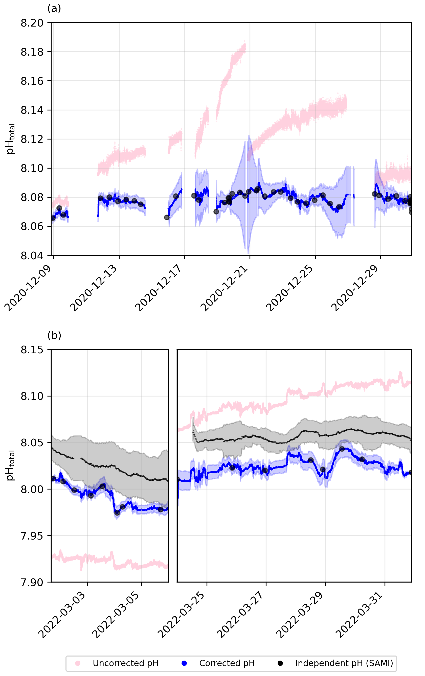
Figure 3 Underway pH drift correction using pH${}_{\mathrm{total}(\mathrm{TA}/\mathrm{DIC})}$ subsamples for (a) cruise SO279 and (b) cruise SO289, with raw pH measurements (pink), corrected pH values and uncertainty from bootstrapping (blue), and subsample pH${}_{\mathrm{total}(\mathrm{TA}/\mathrm{DIC})}$ (black circles). Independent pH from the SAMI sensor is shown in black for the South Pacific cruise (SO289).

2.5 Post-cruise correction

To ensure the reliability of the dataset, an initial screening was conducted to identify and flag unreliable continuous pH data points, primarily attributable to optode stabilisation issues. Specifically, data points recorded during documented periods of particularly rough weather, when air intrusion into the underway system was reported, were flagged as unreliable due to the resulting abrupt and erratic drift patterns that were inconsistent with expected optode and surface ocean pH behaviour.

pH_obs was calculated from TA and DIC UWS discrete samples using PyCO2SYS (Version 1.8.2; Humphreys et al., 2022), with the carbonic acid dissociation constants of Lueker et al. (2000), the bisulfate dissociation constant of Dickson (1990), the total boron-to-chlorinity ratio of Uppström (1974), and the hydrogen fluoride dissociation constant of Dickson and Riley (1979). These calculated values were then aligned with the continuous pH dataset to determine the offset between pH_obs subsamples and the continuous optode-based pH measurements (Fig. 3). A piecewise cubic Hermite interpolating polynomial (PCHIP; Fritsch and Carlson, 1980) was fitted to the offset as a way to continuously correct pH variations across the entire pH time series (Fig. 3). While continuous recalibration of the optode was not possible, a two-point calibration, supplemented by a third-point correction using a CRM, was performed prior to deployment (see Sect. 2.3). Additionally, discrete underway TA and DIC samples, collected twice daily when possible, were used to assess and correct for drift in the optode measurements.

The manufacturer specifies a drift of <0.005 pH units per day at 25 °C, though drift may vary slightly with temperature. During our deployments, seawater temperatures ranged from 13.4 to 22.0 °C in the North Atlantic and from 19.8 to 27.7 °C in the South Pacific. While the cooler North Atlantic conditions may have reduced drift rates slightly, temperatures during the South Pacific cruise were close to or above 25 °C for extended periods, and the full manufacturer-specified drift is likely to have occurred. Even if drift remained at the nominal rate of 0.005 pH units per day, this would amount to a cumulative offset of up to 0.175 pH units over ∼5 weeks (SO279) and 0.28 pH units over ∼8 weeks (SO289), in line with the deviation observed in our raw data (Fig. 3). Notably, even with a recalibration during the cruise, drift before and after that point would still introduce offsets. Thus, over timescales of days and longer, the accuracy of the measurement is dependent on the correction to the TA and DIC samples.

To further assess the robustness of our drift correction, we compared our optode-corrected pH and derived fCO₂ values with independent continuous measurements from autonomous sensors (Figs. S1 and S2 in the Supplement). The corrected optode pH exhibited a lower mean deviation (∼ 0.008) from discrete pH (TA/DIC) measurements than the independent spectrophotometric SAMI sensor (∼0.02 pH units), indicating that our correction effectively minimised drift-related inaccuracies (Fig. S1 in the Supplement). The overall scatter between the optode-corrected and SAMI-measured pH was modest (RMSD = 0.0329), suggesting reasonable consistency despite inherent sensor measurement noise. Similarly, calculated fCO₂ from corrected optode pH showed a larger mean deviation (∼12.7 µatm) compared to directly measured fCO₂ (∼5 µatm; Fig. S2 in the Supplement). The relatively high RMSD (30.76 µatm) reflects variability in calculated fCO₂ arising from uncertainties in alkalinity estimates and carbonate system calculations rather than from fundamental flaws in the optode pH correction itself (Fig. S2 in the Supplement). Thus, these validations collectively confirm that our corrected pH data represent a reliable improvement over raw optode measurements, suitable for robust biogeochemical analysis.

The overall post-cruise correction of pH involved an adjustment of approximately 0.4 to bring the continuous measurements in line with discrete carbonate system observations. However, despite this magnitude of correction, the internal variability within each cycle remains robust, with observed diel fluctuations consistently within ∼0.01. This fine-scale variability aligns with expected temperature-driven pH changes and is distinguishable from random noise. The measurement uncertainty of $\sim \pm \mathrm{0.01}$ means that while some small-scale variations approach the uncertainty threshold, the structured nature of the observed diel trends – rather than random scatter – supports their validity. If these variations were purely noise, we would not expect to see systematic agreement with temperature fluctuations across multiple cycles and regions. To further assess the robustness of these signals, we conducted a signal-to-noise ratio (SNR) analysis (see Supplement). SNR values exceeded 1 when pH was modelled based on temperature (and salinity) in the North Atlantic, indicating that observed diel variability surpassed measurement noise and reflected true environmental signals. In contrast, SNR values remained below 1 in the South Pacific, suggesting that pH variability there was closer to the uncertainty threshold and less clearly distinguishable from noise.

2.6 Estimation of other biogeochemical parameters

TA was estimated for the continuous pH dataset using the empirical equations presented by Lee et al. (2006). For the North Atlantic, the corresponding equation was used (see Fig. S3 in the Supplement):

$$\begin{array}{}\text{(1)}& \begin{array}{rl}{\mathrm{TA}}_{\mathrm{NA}}& =\mathrm{2305}+\mathrm{53.97}\left(\mathrm{SSS}-\mathrm{35}\right)+\mathrm{2.74}(\mathrm{SSS}-\mathrm{35}{)}^{\mathrm{2}}\\ & -\mathrm{1.16}\left(\mathrm{SST}-\mathrm{20}\right)-\mathrm{0.040}(\mathrm{SST}-\mathrm{20}{)}^{\mathrm{2}}.\end{array}\end{array}$$

In contrast, the (sub)tropics equation (SBT, Eq. 2) was applied for the South Pacific region, as the cruise mostly followed the 32.5° S longitude and this equation was determined to offer the best fit to the local sea surface temperature (SST) and sea surface salinity (SSS) equation (see Fig. S3 in the Supplement):

$$\begin{array}{}\text{(2)}& \begin{array}{rl}{\mathrm{TA}}_{\mathrm{SBT}}& =\mathrm{2305}+\mathrm{58.66}\left(\mathrm{SSS}-\mathrm{35}\right)+\mathrm{2.32}(\mathrm{SSS}-\mathrm{35}{)}^{\mathrm{2}}\\ & -\mathrm{1.41}\left(\mathrm{SST}-\mathrm{20}\right)+\mathrm{0.040}(\mathrm{SST}-\mathrm{20}{)}^{\mathrm{2}}.\end{array}\end{array}$$

TA estimates were used together with pH to solve the rest of the marine carbonate system (i.e. DIC and fCO₂) using PyCO2SYS (Version 1.8.2; Humphreys et al., 2022), with the carbonic acid dissociation constants of Lueker et al. (2000), the bisulfate dissociation constant of Dickson (1990), the total boron-to-chlorinity ratio of Uppström (1974), and the hydrogen fluoride dissociation constant of Dickson and Riley (1979).

While direct TA measurements were collected twice daily, their limited temporal resolution made them unsuitable for continuous carbonate system calculations. The empirical TA equations from Lee et al. (2006) provided a high-resolution dataset that allowed for more comprehensive system reconstructions. A comparison of measured and estimated TA values (see Fig. S3 in the Supplement) shows good agreement, with deviations generally within the uncertainty of carbonate system calculations.

2.7 Projected pH variability

The derived parameters pH_temp, pH_sal, and pH_temp,sal were calculated while holding TA and DIC constant at the average values of each diel cycle, where TA was estimated following Lee et al. (2006) and DIC was derived from measured underway pH and estimated TA. This approach allowed us to assess the expected pH response to changes in temperature and salinity alone, without introducing additional assumptions about concurrent variations in carbonate chemistry.

Similarly, pH${}_{\mathrm{TA},f{\mathrm{CO}}_{\mathrm{2}}}$ was computed while holding TA and fCO₂ constant at their daily mean values. fCO₂ was derived from measured pH and estimated TA, ensuring that the calculation reflects equilibrium conditions for given waters with distinct temperature–salinity properties while allowing temperature and salinity to vary independently. This formulation enables direct comparisons of observed pH to expected values under different scenarios, helping to disentangle the relative influences of abiotic drivers (temperature, salinity) versus processes such as air–sea CO₂ exchange and biological activity.

Our approach maintains consistency using a single set of carbonate chemistry parameters (TA and DIC) as the baseline for assessing temperature and salinity influences. While pH is initially used to estimate DIC, the subsequent calculations isolate the effects of temperature and salinity without assuming variability in TA or DIC. This method enables direct comparisons between observed and expected pH, providing a clearer framework for distinguishing abiotic influences from biological processes and air–sea CO₂ exchange.

All calculations were done using the same configuration in PyCO2SYS described in Sect. 2.6.

2.8 Identification of full diel cycles

To account for the influence of geographic location on temporal measurements, timestamps from coordinated universal time (UTC) were converted to local solar time (LST). This conversion was necessary to align time-sensitive data with the true solar position at each measurement location, thereby facilitating more accurate comparisons of environmental data across different geographic regions and improving the analysis of diel processes.

The conversion process involved calculating the mean longitudinal position for each date within the dataset. Subsequently, a time offset was determined based on the average longitude, assuming a standard rate of Earth's rotation. This offset was then applied to the original UTC timestamps, resulting in a modified dataset with timestamps adjusted to reflect LST:

$$\begin{array}{}\text{(3)}& {\mathrm{DateTime}}_{\mathrm{LST}}={\mathrm{DateTime}}_{\mathrm{UTC}}+\left({\displaystyle \frac{{\mathrm{Longitude}}_{\mathrm{mean}}}{\mathrm{15}}}\right).\end{array}$$

Following the conversion into LST, the dataset was further processed to isolate complete diel cycles to ensure that only data representing full 24 h cycles were included. The North Atlantic dataset included 7 complete diel cycles, while the South Pacific dataset included 11 complete diel cycles.

2.9 Uncertainty propagation

2.9.1 Uncertainty in pH measurements and post-correction

To provide a comprehensive uncertainty estimate, we considered multiple sources of potential error. The manufacturer-reported accuracy (±0.05 for pH 7.5–9.0, ±0.1 for pH 7.0–7.5) represents a systematic bias that was addressed through calibration against discrete CRM samples and is not appropriate for inclusion as a random uncertainty. Likewise, the reported precision (±0.003 at pH 8.0) reflects the repeatability of the measurements but does not quantify the full range of uncertainty for error propagation. The final uncertainty in pH measurements was estimated by combining uncertainties from two main sources: (1) the uncertainty in the TA and DIC measurements used to calculate pH_obs and (2) the correction of the UWS pH measurements using pH_obs.

First, the precision in TA and the precision in DIC were determined based on the RMSE from repeated measurements of a known standard water sample in the laboratory (NIOZ; 0.92 and 1.95 µmol kg⁻¹, respectively). Then a Monte Carlo simulation was applied to the calculated pH_obs to obtain a pH_RMSE value for each subsample pH_obs.

Next, the pH measurements obtained from the optode were corrected using pH_(TA, DIC) from the discrete measurements of TA and DIC. The uncertainty in the pH correction was assessed using a bootstrapping approach (n=1000 iterations), where a fraction (50 %) of the discrete samples was randomly omitted in each iteration and the selected fraction of the discrete samples varied within its own pH_RMSE.

The variation in each subsample's pH_obs captured the likely variability in TA and DIC measurements, while omitting different subsets of data allowed for the estimation of how sensitive the pH correction is to which set of subsamples is used for calibration.

2.9.2 Uncertainty in pH diel patterns

To ensure that the observed patterns in pH over the full 24 h cycles were not artefacts of sampling bias or other anomalies, a Monte Carlo simulation (n=1000 iterations) was employed on each diel cycle's hourly data analysis. This simulation randomly selected 50 % of the data points for each hour (i.e. 50 % of 120 hourly measurements for the North Atlantic dataset and 50 % of 240 hourly measurements for the South Pacific dataset), repeatedly calculating the mean pH to assess the consistency and robustness of the hourly trends. This component of the uncertainty proved insignificant (i.e. errors bars were smaller than the symbols in Figs. 4 and 5).

2.10 CO₂ air–sea flux dynamics

Air–sea CO₂ fluxes were computed based on the following relationship:

$$\begin{array}{}\text{(4)}& F=k_{\mathrm{w}}\times K_{\mathrm{0}}\times (p{\mathrm{CO}}_{{\mathrm{2}}_{\mathrm{SW}}}-p{\mathrm{CO}}_{{\mathrm{2}}_{\mathrm{air}}}),\end{array}$$

where F represents the flux of CO₂ across the air–sea interface; k_w is the gas transfer velocity; K₀ is the solubility constant; $p{\mathrm{CO}}_{{\mathrm{2}}_{\mathrm{SW}}}$ is the partial pressure of CO₂ in seawater, representing the concentration of dissolved CO₂ that is in equilibrium with the atmosphere; and $p{\mathrm{CO}}_{{\mathrm{2}}_{\mathrm{air}}}$ is the partial pressure of CO₂ in the atmosphere above the ocean surface. For the fluxes, a positive value shows that the ocean acts as a source (i.e. releasing CO₂ to the atmosphere), while a negative value shows it acts as a sink (i.e. absorbing CO₂ from the atmosphere). The parameterisation from Ho et al. (2006) was used to determine the gas transfer velocity. All fluxes were computed using the pySeaFlux package (v2.2.2; Fay et al., 2021).

Flux calculations were performed for each complete diel cycle, followed by the computation of the mean flux for each cycle. Additionally, the mean flux for the diel cycle was also calculated from the daily mean inputs (wind speed, temperature, salinity, and pCO₂) and specifically computed for the hours 12:00 a.m. and 12:00 p.m. (LST) to examine temporal variations within each cycle (Fig. 9).

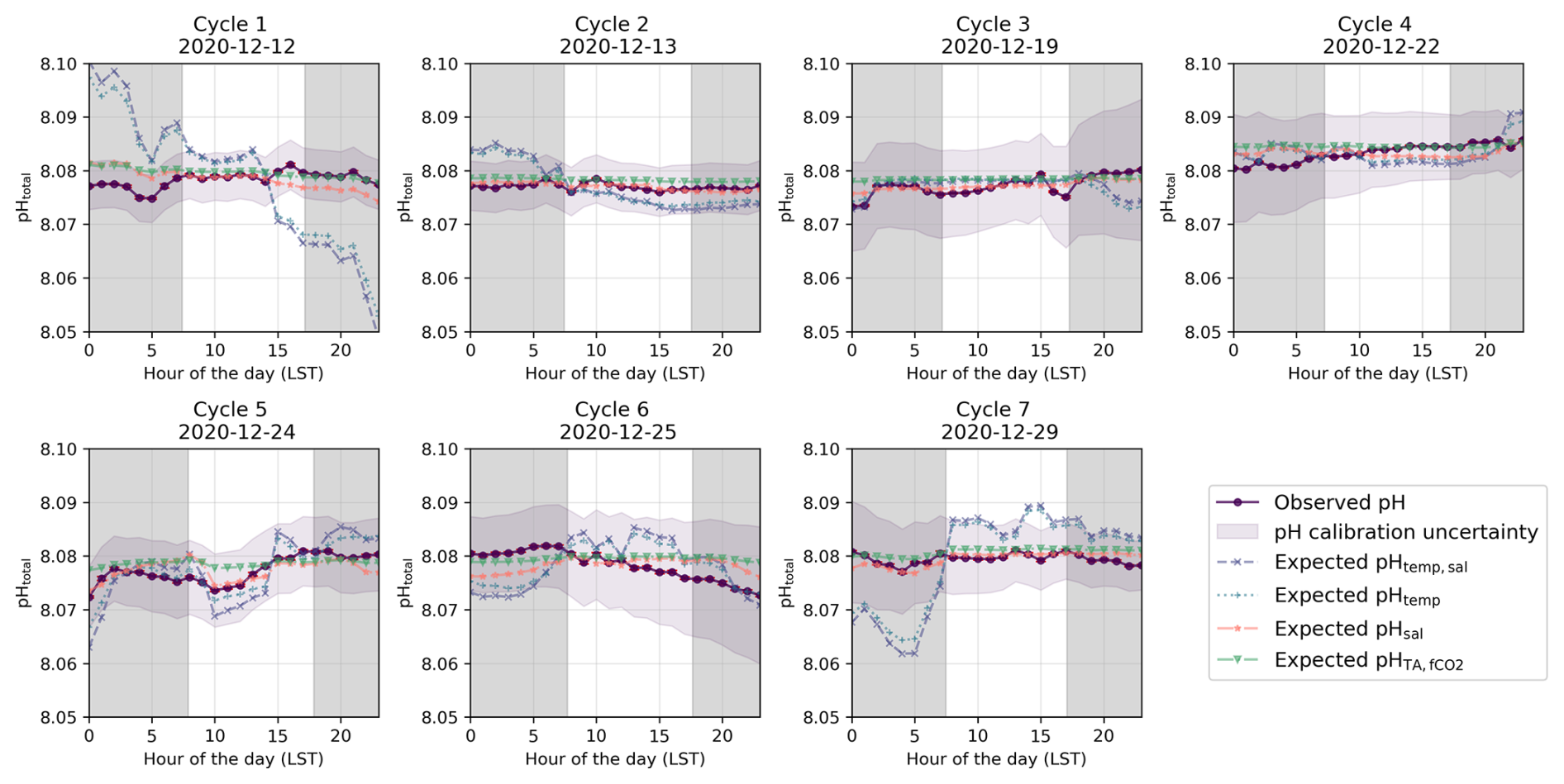
Figure 4 Identified diel cycles for cruise SO279 in the North Atlantic Ocean. Dark purple lines show observed pH (pH_obs). The remainder shows expected pH using varying temperature and salinity (pH_temp,sal; dashed light purple lines), varying temperature alone (pH_temp; dotted blue lines), varying salinity alone (pH_sal; dashed orange lines), and constant TA and fCO₂ (pH${}_{\mathrm{TA},f{\mathrm{CO}}_{\mathrm{2}}}$; dashed green lines). Grey areas are night hours.

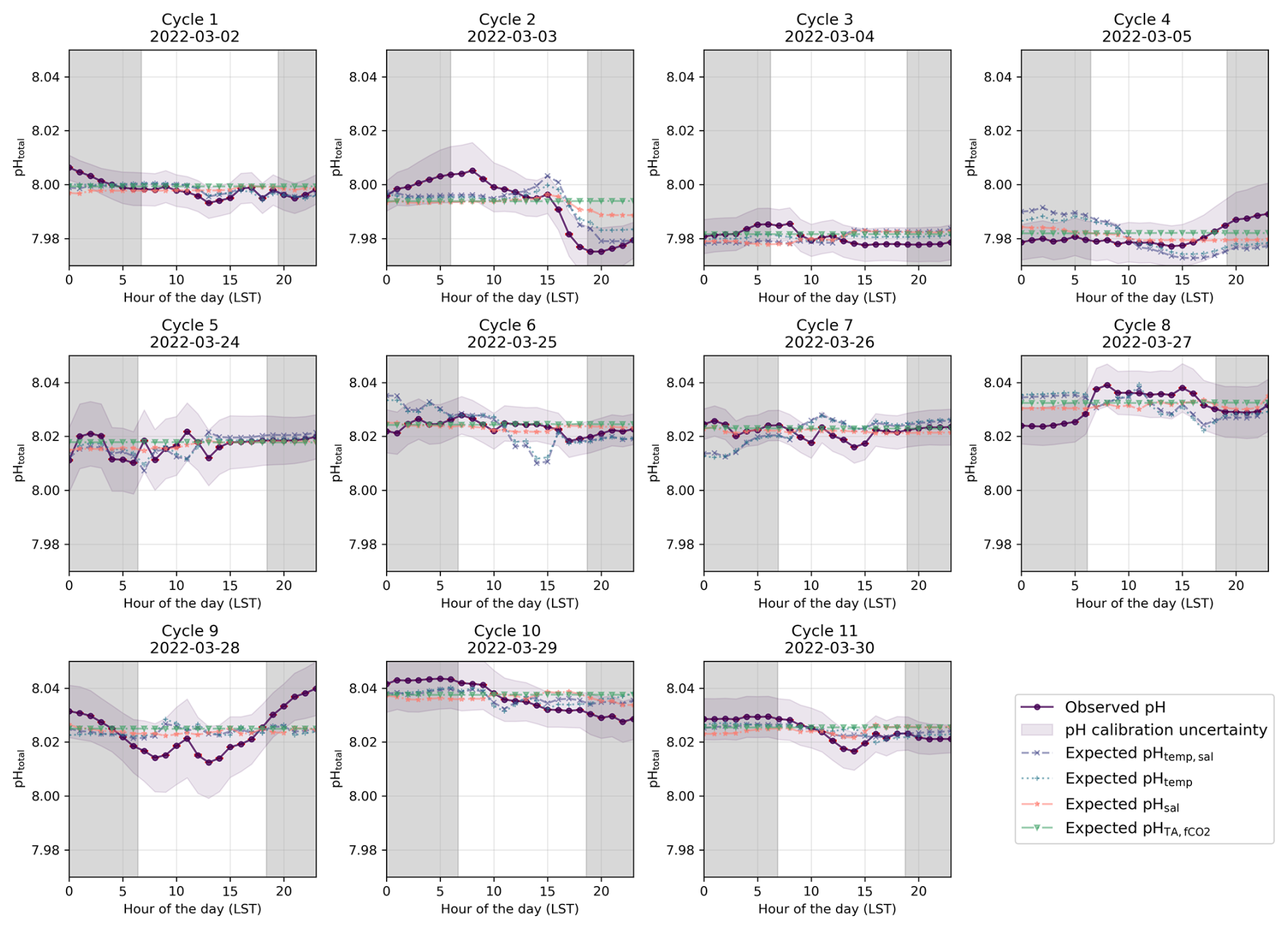
Figure 5 Identified diel cycles for cruise SO289 in the South Pacific Ocean. Dark purple lines show observed pH (pH_obs). The remainder shows expected pH using varying temperature and salinity (pH_temp,sal; dashed light purple lines), varying temperature alone (pH_temp; dotted blue lines), varying salinity alone (pH_sal; dashed orange lines), and constant TA and fCO₂ (pH${}_{\mathrm{TA},f{\mathrm{CO}}_{\mathrm{2}}}$; dashed green lines). Grey areas are night hours.

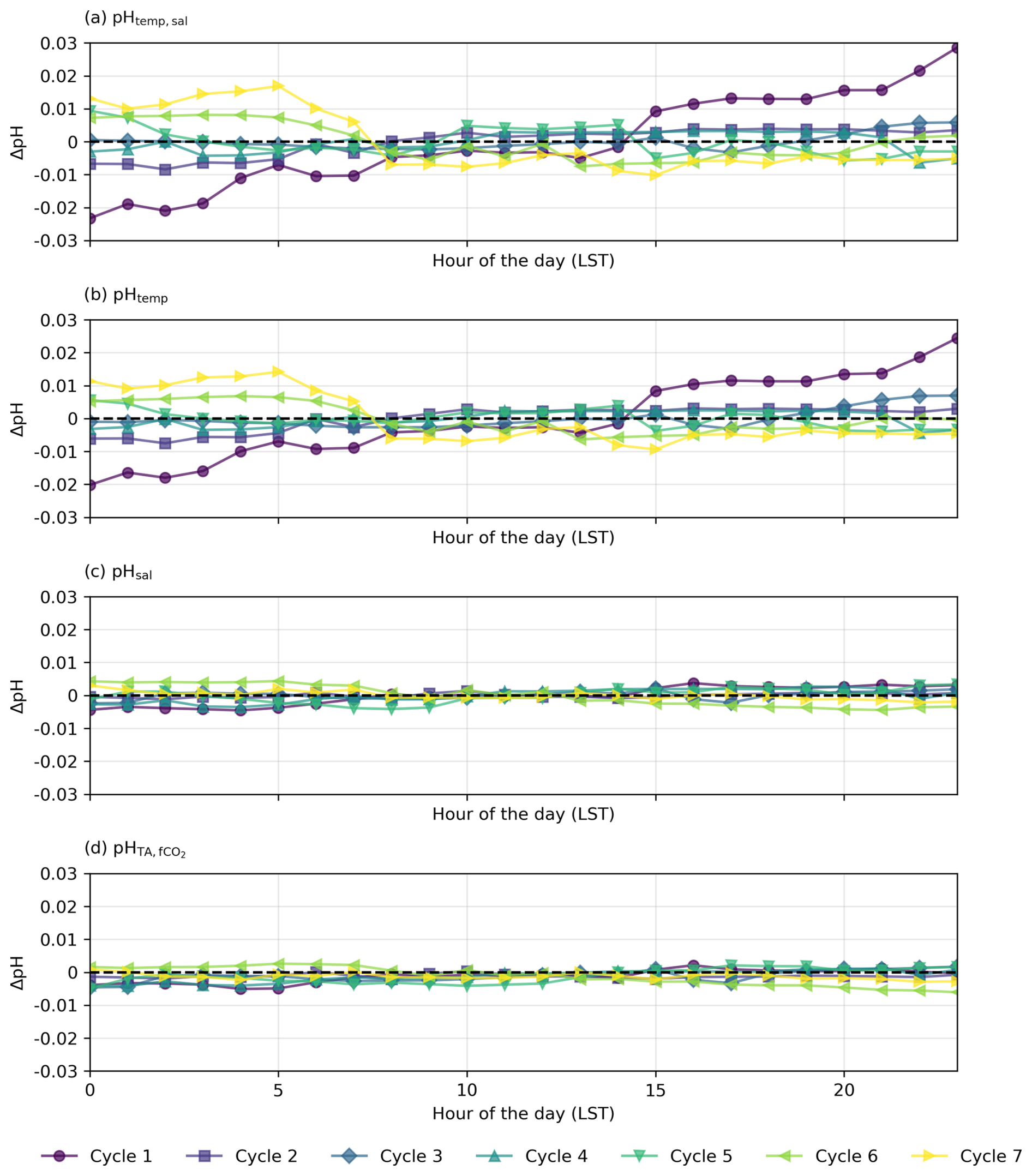
Figure 6 Residual plots for diel cycles in the North Atlantic, illustrating the differences (ΔpH) between observed pH measured by the optode (pH_obs) and (a–c) pH calculated from constant TA and DIC with (a) varying temperature and salinity (pH_temp,sal), (b) varying temperature only (pH_temp), and (c) varying salinity only (pH_sal) and (d) constant TA and fCO₂ with varying temperature and salinity. Horizontal dashed lines at y=0 indicate no deviation between observed and calculated pH.

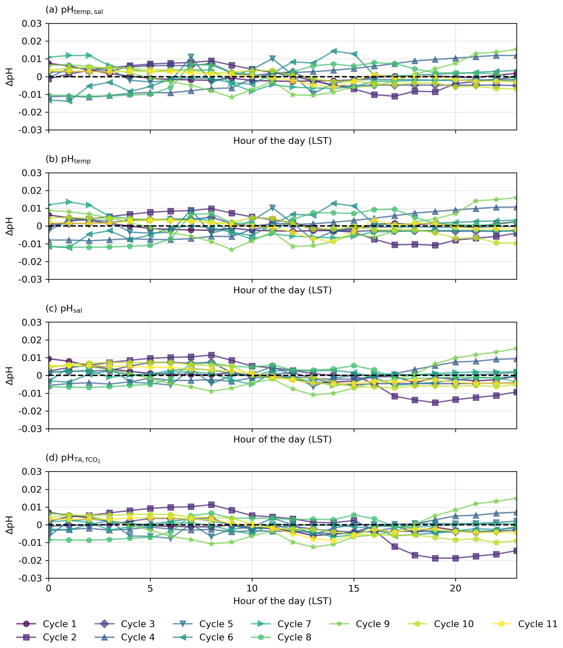
Figure 7 Residual plots for diel cycles in the South Pacific, illustrating the differences (ΔpH) between observed pH measured by the optode (pH_obs) and (a–c) pH calculated from constant TA and DIC with (a) varying temperature and salinity (pH_temp,sal), (b) varying temperature only (pH_temp), and (c) varying salinity only (pH_sal) and (d) constant TA and fCO₂ with varying temperature and salinity. Horizontal dashed lines at y=0 indicate no deviation between observed and calculated pH.

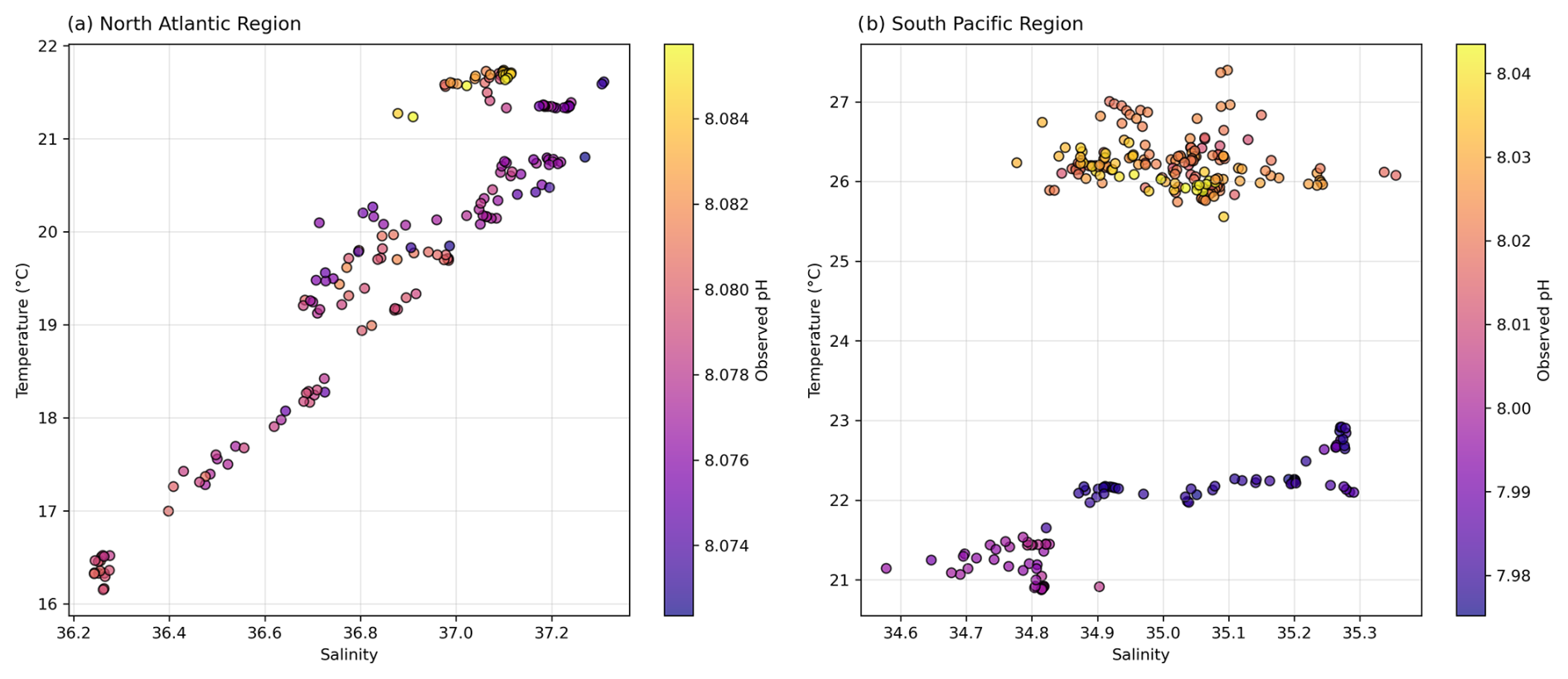
Figure 8 $T/S$ diagram with observed pH for (a) the North Atlantic region and (b) the South Pacific region.

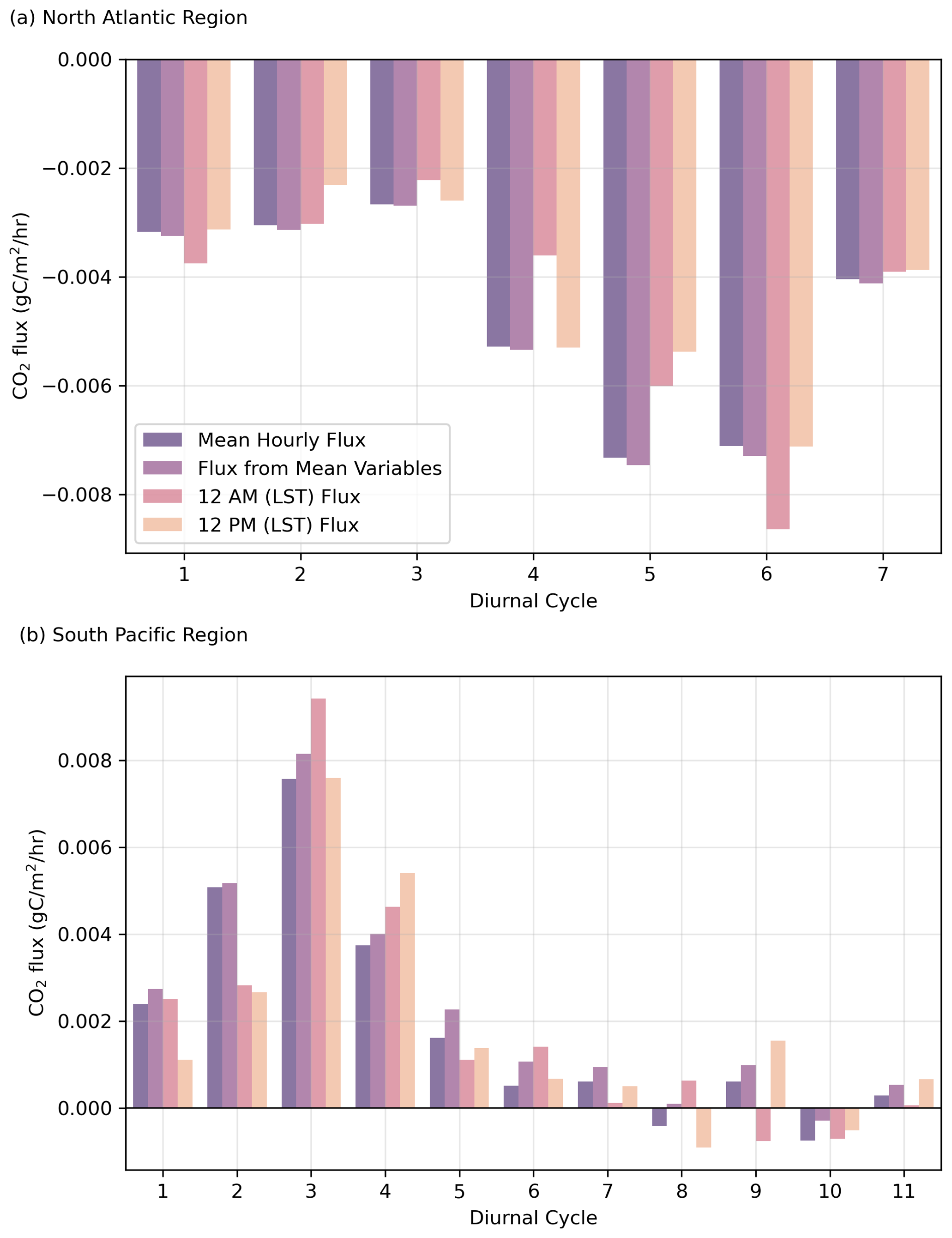
Figure 9 Sensitivity analysis of mean CO₂ flux compared to flux calculated from mean inputs, fluxes for 12:00 a.m. (LST) and fluxes for 12:00 p.m. (LST). The top panel (a) shows cruise SO279 in the North Atlantic, while the bottom panel (b) shows cruise SO289 in the South Pacific.

3 Results and discussion

We first analyse the effects of temperature and salinity on pH across different diel cycles and regions (Sect. 3.1) using high-resolution pH data enabled by our novel optical measurement system. We examine the pH expected from temperature and salinity variations alone (pH_temp,sal), disregarding changes in TA or DIC. If pH_obs (i.e. corrected underway pH measurements using discrete TA and DIC subsamples) aligns with pH_temp,sal, it suggests that recent temperature changes, such as day–night cycles, primarily control pH. In this context, “recent” is relative to the air–sea CO₂ equilibration timescale, i.e. temperature change that happened recently enough that its effect on pH has not been modified by subsequent gas exchange. Next, we assess the influence of hydrographic variations on pH by considering pH${}_{\mathrm{TA},f{\mathrm{CO}}_{\mathrm{2}}}$, which accounts for constant fCO₂ instead of DIC alongside constant TA and varying temperature and salinity. Alignment of pH_obs with pH${}_{\mathrm{TA},f{\mathrm{CO}}_{\mathrm{2}}}$ indicates that slower or long-ago processes control pH. For example, an observed change in temperature may be due to spatial variability, with the ship passing through different waters with distinct temperature–salinity properties that have had different temperatures for long enough to re-equilibrate with atmospheric CO₂. By leveraging the high-frequency resolution of our measurement system, we then explore the role of biological activity and its interaction with abiotic factors by looking at the discrepancies between pH_obs and both pH_temp,sal and pH${}_{\mathrm{TA},f{\mathrm{CO}}_{\mathrm{2}}}$ (Sect. 3.2). Finally, we distinguish between temporal and spatial variability in our measurements (Sect. 3.3), considering implications for air–sea CO₂ equilibration timescales at fine spatio-temporal scales (Sect. 3.4).

3.1 Influence of temperature and salinity

3.1.1 Basin-scale comparison

The diel cycles of pH observed in the North Atlantic and South Pacific oceans are significantly influenced by temperature. In the North Atlantic, observed pH stays within ±0.01 of pH_temp,sal, supporting the role of temperature and salinity in driving pH changes (Fig. 6). However, in the South Pacific, where SNR values for temperature- and salinity-driven pH changes remain below 1, observed fluctuations may not exceed measurement noise, making it uncertain whether these variations reflect true environmental signals or instrument variability (Fig. 7; Table S6 in the Supplement). Despite this, the systematic nature of diel fluctuations – seen across multiple cycles and their correlation with expected temperature-driven trends – suggests variations are meaningful rather than random.

Salinity alone does not appear to strongly influence pH in any observed cycle. For both ocean basins, pH_sal typically remains close to the mean pH of each cycle, rather than impacting the observed pH significantly. This consistency suggests that daily salinity variations do not exert a primary influence on the observed pH (Figs. 4, 5, 6c, 7c; Tables S1 and S2 in the Supplement). Thus, the rest of this section focuses on the effect of temperature on the observed pH.

In the North Atlantic, the observed variability in pH generally matches the calculated pH_temp and pH_temp,sal, with most cycles' residuals within ±0.01 (Figs. 4 and 6a and b, Cycles 2, 3, 4, 5, and 6). This agreement suggests that temperature and salinity together explain most of the observed short-term variations. However, some cycles show more pronounced deviations. Cycle 3 demonstrates a particularly strong alignment between observed pH and expected pH_temp,sal throughout the day (mean residuals < 0.001; Figs. 4, 6a and b), while Cycle 4 also exhibits minimal variation (residuals −0.007 to 0.003; Fig. 4).

In the South Pacific, pH variability follows a different pattern, While some cycles (e.g. Cycles 1, 3, 4, and 6) show similar agreement between observed pH and pH_temp,sal (Fig. 5), overall, the influence of temperature appears weaker than in the North Atlantic. The SNR analysis (see Sect. S1 in the Supplement) confirms this, with North Atlantic temperature-driven pH fluctuations exceeding noise (SNR = 1.39 for pH_temp,sal, 1.20 for pH_temp), while all pH variations in the South Pacific remain below SNR = 1 (see Tables S1 and S2 in the Supplement). This suggests that in the South Pacific, observed fluctuations may be more influenced by noise than by real temperature-driven variability. However, the persistence of systematic diel fluctuations suggests that meaningful signals are still present.

The physical oceanographic context of each basin likely contributes to these differences. In the North Atlantic, significant mixing due to ocean currents, eddies, and upwelling introduces substantial variability in temperature, salinity, and pH across different waters with distinct temperature–salinity properties (Fig. 6a and b; see Fig. S8 in the Supplement). The Gulf Stream and North Atlantic Drift contribute to this complexity, which may help maintain stronger temperature-driven pH changes by continuously exposing surface waters to variable thermal forcing (Liu and Tanhua, 2021). In contrast, the South Pacific exhibits more predictable hydrographic dynamics, driven largely by advection and mixing within large-scale gyres and trade wind systems (Vallis, 2017). This results in a more stable and homogeneous water column, where observed pH fluctuations remain closer to the measurement uncertainty (Fig. 7).

3.1.2 Diel pH variability

Beyond the basin-scale differences, a key feature of the observed pH cycles is the variability between daytime and nighttime conditions. In both basins, temperature changes between day and night are expected to drive corresponding pH shifts due to the temperature dependence of the carbonate system.

In the North Atlantic, observed pH generally follows expected temperature-driven changes, with pH_temp and pH_temp,sal showing higher values at night and lower values during the day due to the inverse relationship between temperature and pH (Figs. 4, 6). For example, in Cycles 3 and 6, the residuals between observed and expected pH remain small throughout the day, reinforcing the dominance of temperature as a control mechanism. However, in some cycles (e.g. Cycle 1), nighttime pH remains elevated beyond what would be expected from temperature alone, suggesting the influence of additional processes such as biological activity or air–sea CO₂ exchange.

In the South Pacific, similar diel patterns are present but exhibit greater variability across cycles. Some cycles (e.g. Cycle 8) show clear daytime decreases and nighttime increases in pH, consistent with temperature-driven changes (Fig. 5). However, in other cases (e.g. Cycle 9), observed pH departs from the expected diel pattern, indicating that other factors may be influencing short-term variability.

The persistence of nighttime pH anomalies in both basins raises questions about equilibration timescales. While temperature-driven changes in pH and fCO₂ occur rapidly in response to solubility and speciation shifts, CO₂ equilibration between the atmosphere and ocean occurs over much longer timescales (weeks to months; Jones et al., 2014). This means that pH adjustments due to temperature occur almost instantly, but whether they persist over a full diel cycle depends on the history of the hydrographic properties. If waters have recently equilibrated with the atmosphere, their pH should closely follow pH_temp,sal. However, if these waters have undergone rapid temperature shifts without sufficient time for equilibration, observed pH may diverge from temperature-based expectations. This highlights the interplay between rapid thermodynamic effects and longer equilibration processes, particularly in regions like the North Atlantic, where mixing introduces additional complexity.

Ultimately, our observations suggest that while temperature is a dominant driver of diel pH changes, the extent to which these changes persist overnight depends on the physical characteristics of the surface waters and their equilibration history. In the North Atlantic, where mixing is more dynamic, the system appears to re-equilibrate more readily, whereas in the South Pacific, longer equilibration timescales may contribute to greater deviations from expected pH patterns.

3.2 Influence of biological activity

While temperature and salinity effects on pH are addressed in Sect. 3.1, deviations from expected patterns may be shaped by biological processes. The process of photosynthesis during daylight consumes CO₂, leading to a rise in pH, whereas respiration and decomposition at night, which release CO₂, lower pH (Falkowski, 1994; Falkowski and Raven, 2013). The balance between photosynthesis and respiration hence affects pH and should result in a diel pH cycle. However, biological signals in the open ocean are often weaker than in coastal or upwelling regions due to lower phytoplankton biomass and primary production rates (Behrenfeld and Falkowski, 1997; Johnson et al., 2010). As a result, strong diel biological pH signals are not typically expected in oligotrophic oceanic waters. These biological processes can also influence the rate at which CO₂ equilibrates between the ocean and atmosphere. For instance, intense photosynthetic activity during daylight hours can rapidly deplete seawater pCO₂ in surface waters, potentially accelerating seawater CO₂ uptake from the atmosphere. Conversely, nighttime respiration can increase pCO₂, slowing the outgassing process and thus extending the equilibration timescale. However, given an equilibration timescale of months, these day and night changes likely get averaged out over longer periods, resulting in an overall steady-state CO₂ flux and pH when observed over longer temporal scales.

These biological processes are particularly evident in some cycles from the North Atlantic where the expected pH_temp,sal changes due to temperature and salinity do not align with the observed data but do follow the distribution expected from biological activity (Fig. 4). However, the strength of these pH variations should be interpreted with caution, as biological activity in open-ocean regions tends to be relatively low (Longhurst, 2007). The North Atlantic subtropical gyre, for instance, has low rates of primary productivity (Baines et al., 1994; Tilstone et al., 2003), which suggests that biologically driven pH variations would be relatively small. This is especially evident for Cycle 1, which shows an increase in pH during daylight hours and a decrease in pH during night hours, with a peak in pH in late afternoon and the lowest pH occurring in the early morning before sunrise (Fig. 4). Other cycles likely reflect the combined impact of biological processes and temperature effects, as the observed pH does not fully align with the distribution expected from any of the temperature, salinity, or biological activity (Figs. 4 and 6). In the South Pacific Ocean, some cycles show significant variability within pH_obs that are not mirrored by the expected pH_temp,sal changes (Fig. 5, Cycles 2 and 8). For example, Cycle 2 exhibits significant deviations in pH with higher observed values in the morning and a drop in the afternoon (Fig. 5). Although this suggests a potential biological influence, the SNR values remain below 1 across all expected pH estimates, making it unclear whether the observed fluctuations are truly driven by biological activity or simply fall within the instrument's noise threshold (Table S6 in the Supplement).

The interplay between photosynthesis during the day and respiration at night, with possible contributions of other biological processes, may be behind the more pronounced peaks and troughs of Cycles 2 and 9 (Fig. 6; Duarte and Agusti, 1998). Nitrogen fixation consumes hydrogen ions, increasing pH, whereas denitrification releases hydrogen ions, thereby decreasing pH (Richardson, 2000; Zehr and Kudela, 2011). However, without nutrient and oxygen data, we cannot directly assess whether these processes also impacted the observed pH.

Although biological activity likely accounts for some variability, not all cycles exhibit the same residual, presumably biotic, pattern of variation (Figs. 4 and 5). This aligns with expectations, as phytoplankton biomass and primary productivity in open-ocean regions can be highly variable, and biological impacts on carbonate chemistry are typically more pronounced in coastal or upwelling systems (Duarte and Agusti, 1998; Williams and Follows, 2003). Moreover, the SNR results indicate that in the North Atlantic, temperature-driven processes dominate short-term pH variability, while the contribution of biological activity remains unclear due to overlapping influences (see Table S1 in the Supplement). In the South Pacific, where all signals fall below the noise threshold (SNR <1; Table S6 in the Supplement), the observed pH fluctuations may be driven by measurement uncertainty rather than a clear biological or temperature-driven signal.

This variability further complicates assessments of air–sea CO₂ equilibration, as localised biological conditions may transiently alter CO₂ dynamics, influencing the timescale for reaching equilibrium. This is more obvious in the South Pacific, where some cycles display more pronounced nighttime stability (Fig. 5, Cycles 3, 6, 7, and 11), while others have noticeable daytime fluctuations that could align with photosynthetic activity, which typically increase during daylight hours (Fig. 5, Cycle 8; Duarte and Agusti, 1998; Raven and Johnston, 1991). Cycle 8 in the South Pacific shows a peak in observed pH around midday, likely due to increased photosynthesis, followed by a decrease in the evening (Fig. 5). Other cycles do not show this pattern as clearly (i.e. they even show a decrease in pH during the day), suggesting that, for some cycles, respiration may also dominate over photosynthesis during the daytime (Fig. 5). For example, Cycle 9 displays significant variations in pH throughout the day, with notable decreases during daylight hours (Fig. 5). Additionally, as some cycles appear to conform to temperature-based pH expectations, the only minor deviations observed suggest biological activity is minor or represents a balanced biological system where photosynthesis and respiration are in near-equilibrium (Fig. 5, Cycles 3 and 6).

Despite the strong impact of both abiotic and biotic factors on pH, some cycles exhibit fine-scale trends that cannot be solely attributed to temperature fluctuations or biological activity. The fine-scale trends observed, especially in Cycles 1 and 7 (Fig. 4), exceed what can be attributed to temperature-induced changes alone and cannot be explained by biological activity, given the atypically high carbon fixation rates required to explain the pH offsets (Basu and Mackey, 2018; Wang et al., 2023). Indeed, the required biological carbon fixation would need to exceed 687 mg C m⁻³ d⁻¹ to explain the offset (Sect. S2 in the Supplement). Typical rates in open-ocean waters are much lower, generally ranging from 50 to 150 mg C m³ d⁻¹ in nutrient-poor regions and reaching up to 1000 C m⁻³ d⁻¹ in upwelling zones during phytoplankton blooms, which is not the case here (Basu and Mackey, 2018; Wang et al., 2023).

Comparing the impact of biological activity based on the offsets between pH_temp and pH_obs with chlorophyll a fluorescence data also shows no clear pattern (see Figs. S4 and S5 in the Supplement). This is expected as fluorescence does not necessarily reflect instantaneous photosynthetic activity. Instead, fluorescence primarily indicates the presence and abundance of phytoplankton. Therefore, while fluorescence can provide insights into the overall biomass of phytoplankton, it does not directly correlate with photosynthesis and respiration. The absence of a clear correlation between fluorescence and the daily pH cycle, with some cycles even showing a decrease in pH during daytime, confirms that the influence of waters with distinct temperature–salinity properties is important in shaping the local high-resolution pH profiles.

3.3 Variability and stability in spatio-temporal pH patterns

As examined in Sect. 3.1, considerable spatial variability is observed in the North Atlantic (Fig. 8; see Fig. S8 in the Supplement), and this heterogeneity introduces complexity into deciphering the relative contributions of abiotic and biotic factors to pH fluctuations (Gruber and Sarmiento, 2002). Residual plots for the North Atlantic suggest that the observed discrepancies between pH_obs and both pH_temp and pH_temp,sal are insignificant, indicating that variability in surface water characteristics – which include but are not limited solely to temperature and salinity – does not dominate the observed pH variability (Figs. 6 and 8; Dumousseaud et al., 2010). The SNR results further confirm that temperature-driven pH fluctuations are real signals in this region (SNR >1; Table S1 in the Supplement), supporting their role as key drivers of diel pH variability. Therefore, the hourly fluctuations in pH_obs and the observed discrepancies between pH_obs and pH${}_{\mathrm{temp}/\mathrm{sal}}$ across various cycles in this ocean basin may not be attributed to pronounced spatial variability (Fig. 4). The $T/S$ diagram also demonstrates this spatial variability, showing a wide range of pH values correlated with differing salinity and temperature profiles across waters with distinct temperature–salinity properties (Fig. 8), reinforcing the notion that spatial dynamics do not significantly influence pH variation in this region. This is also supported by the relative stability observed in Cycle 4, where the ship's consistent positioning (i.e. on station) highlights the role of temporal variability rather than spatial variability (see Fig. S6 in the Supplement). Although water could still be moving spatially around the ship, the variability could be due to some degree to different waters rather than being limited to true in situ temporal variability.

In contrast, the South Pacific cruise predominantly exhibits a stable transit through more homogeneous surface waters as no SST gradient is observed, although it is not entirely free from disruptions (see Fig. S7 in the Supplement; Qu and Lindstrom, 2004). This suggests a limited role of interactions between diverse surface waters. Despite the hourly fluctuations observed, all diel cycles in the South Pacific tend to cluster closely around the mean pH for their respective 24 h periods, reflecting substantial stability within each cycle but considerable variability across different days, particularly evident among consecutive cycles (Fig. 5). This underscores a clear temporal delineation of diel cycles influenced by DIC changes (Fig. 5). However, the SNR results indicate that all expected pH fluctuations in this region remain below the uncertainty threshold (SNR <1; Table S6 in the Supplement), making it difficult to determine whether observed fluctuations reflect true environmental variability or are primarily within the measurement uncertainty.

3.4 Implications for air–sea CO₂ fluxes

Our findings indicate that while temperature and salinity predominantly govern diel pH fluctuations, additional variability arises from surface water dynamics and biological activity. Temperature rapidly affects pH, but the slower rate of CO₂ equilibration with the atmosphere moderates its impact on air–sea CO₂ fluxes. Although biological processes markedly influence daily pH cycles, they do not fully account for the observed variability, especially in cases where unusually high carbon fixation rates would be required to explain observed pH (Sect. 3.2). Notably, the North Atlantic acted as a net sink of CO₂, whereas the South Pacific was a net source to the atmosphere during the study period.

CO₂ fluxes were calculated for each complete diel cycle (Fig. 9). The flux calculations were performed by computing the mean flux for each cycle from daily mean inputs (wind speed, temperature, salinity, and pCO₂) and specifically for the hours 12:00 a.m. and 12:00 p.m. (LST) to examine temporal variations within each cycle (Fig. 9). Despite different methods of calculation, the CO₂ fluxes remained relatively consistent, indicating that the variations in pH and thus CO₂ flux do not significantly affect the air–sea CO₂ exchange in either basin.

This consistent result shows that, despite the processes influencing pH in these two ocean basins during the study period, air–sea CO₂ exchange over longer timescales (e.g. months) can dampen short-term pH variability, resulting in relatively low variability across short spatio-temporal scales (km d⁻¹).

4 Conclusions

High-resolution pH data enabled by our novel optical measurement system provide valuable insights into the complex and variable nature of surface ocean pH. Our observations in the North Atlantic and South Pacific show that pH fluctuates on diel and hourly timescales, with variations driven not only by temperature but also by the interplay between waters with distinct temperature–salinity properties and biological activity. These factors do not operate in isolation, making it difficult to attribute pH changes to a single dominant driver.

Although the processes governing pH variability are well-understood, our high-frequency measurements demonstrate the challenge of disentangling their contributions at fine spatial and temporal scales. This underscores the importance of continuous, high-frequency measurements, which reveal the heterogeneity in surface pH that lower-resolution datasets might miss. In both basins, the close correlation between pH${}_{\mathrm{TA},f{\mathrm{CO}}_{\mathrm{2}}}$ and observed pH across diel cycles suggests that air–sea CO₂ exchange plays a key role in stabilising pH despite temperature fluctuations. The observed pH stability implies that the ship primarily encountered waters that had already equilibrated with atmospheric CO₂, reinforcing the idea that temperature-driven pH changes alone are not always sufficient to explain variability in surface ocean carbonate chemistry.

While our results indicate that fine-scale variability in these regions was relatively subtle – and may not significantly impact large-scale assessments – this insight could only be gained through high-resolution observations. This approach not only reveals the complexity of pH regulation but also provides valuable insight into the fine-scale physical and biological interactions that shape surface ocean chemistry. Importantly, although lower-resolution datasets may be sufficient for capturing broad-scale patterns in surface ocean CO₂ chemistry, our findings highlight the critical role of high-frequency measurements in refining regional understanding and improving predictive models of ocean acidification and air–sea gas exchange.