Carbon sequestration in different urban vegetation types in Southern Finland

Many cities seek carbon neutrality and are therefore interested in the sequestration potential of urban vegetation. However, the heterogeneous nature of urban vegetation and environmental conditions limits comprehensive measurement efforts, setting expectations for carbon cycle modelling. In this study, we examined the performance of three models – the Jena Scheme for Biosphere–Atmosphere Coupling in Hamburg (JSBACH), the Lund–Potsdam–Jena General Ecosystem Simulator (LPJ-GUESS), and the Surface Urban Energy and Water Balance Scheme (SUEWS) – in estimating carbon sequestration rates in both irrigated and non-irrigated lawns, park trees (Tilia cordata), and urban forests (Betula pendula) in Helsinki, Finland. The test data included observations of various environmental parameters and component fluxes such as soil moisture and temperature, sap flow, leaf area index, photosynthesis, soil respiration, and net ecosystem exchange. Our analysis revealed that these models effectively simulated seasonal and annual variations, as well as the impacts of weather events on carbon fluxes and related factors. However, the validation of the absolute level of modelled fluxes proved difficult due to differences in the scale of the observations and models, particularly for mature trees, and due to the fact that net ecosystem exchange measurements in urban areas include some anthropogenic emissions. Irrigation emerged as a key factor often improving carbon sequestration, while tree-covered areas demonstrated greater carbon sequestration rates compared to lawns on an annual scale. Notably, all models demonstrated similar mean net ecosystem exchange over the urban vegetation sector studied on an annual scale over the study period. However, compared to JSBACH, LPJ-GUESS exhibited higher carbon sequestration rates in tree-covered areas but lower rates in grassland-type areas. All models indicated notable year-to-year differences in annual sequestration rates, but since the same factors, such as temperature and soil moisture, affect processes both assimilating and releasing carbon, connecting the years of high or low carbon sequestration to single meteorological means failed. Overall, this research emphasizes the importance of integrating diverse vegetation types and the impacts of irrigation into urban carbon modelling efforts to inform sustainable urban planning and climate change mitigation strategies.

1 Introduction

The majority of combustion of fossil fuels occurs within urban environments, contributing an estimated 40 %–50 % of global anthropogenic greenhouse gas emissions (Marcotullio et al., 2013). Cities worldwide are actively engaged in climate change mitigation efforts, formulating strategies to decrease their anthropogenic emissions (Rosenzweig et al., 2010; Reckien et al., 2014; Mitchell et al., 2022; Ferrini et al., 2020) and striving for carbon neutrality. The pursuit of carbon neutrality has highlighted the role of urban vegetation, perceived as a cost-effective method with minimal management requirements, in offsetting emissions. Moreover, green spaces in urban areas offer diverse ecosystem services, such as mitigating excessive water flow (Berland et al., 2017) and the urban heat island effect (Rahman et al., 2020), as well as improving human health and well-being (Wolf et al., 2020; Cuthbert et al., 2022).

As a result, understanding and quantifying carbon storage and fluxes in urban green areas and understanding the impact of management practices on carbon are necessary to mitigate climate change through carbon-smart design. As changes in carbon fluxes represent changes in the overall ecosystem functioning, these can also be used to indicate some of the other ecosystem services provided. In urban green spaces, carbon dynamics are influenced by a wide range of factors, including land use and the selection of species, the intensity of use and management, and microclimatic conditions. The heterogeneity of the urban environment creates variation in the conditions for carbon sequestration, most importantly in temperature, humidity, CO₂ concentration, and radiation, as well as in fertility and soil conditions (Bezyk et al., 2018). It is well-known that these local effects modify the urban carbon fluxes by altering, for example, the length of the growing season (Imhoff et al., 2004; Wohlfahrt et al., 2019), tree growth (Dahlhausen et al., 2018), and soil conditions (Edmondson et al., 2016). In addition to creating local heterogeneity, these factors also vary from year to year, and the variation will be even more pronounced under climate change since extreme climatic events are more frequent and last for longer periods (Kim et al., 2018). Hence, warming could reduce tree growth (Meineke et al., 2016) and, remarkably, increase soil respiration (Rustad et al., 2000), further impacting inter-annual variation in carbon dynamics.

The heterogeneity of urban green spaces, coupled with the year-to-year variability in weather patterns, poses challenges for empirically estimating carbon sequestration. Consequently, physiologically oriented ecosystem models are needed to quantify both the present extent and the future development of carbon sequestration and at the same time, potentially some other ecosystem services. Based on extensive empirical data in native and managed ecosystems, many comprehensive models on photosynthesis (Mäkelä et al., 2004; Hari et al., 2017), plant internal carbon balance (Schiestl-Aalto et al., 2019), net ecosystem exchange of forests (Lindeskog et al., 2021; Bergkvist et al., 2023) and agricultural fields (Ma et al., 2023; Lindeskog et al., 2013), and land surface models such as the Jena Scheme for Biosphere–Atmosphere Coupling in Hamburg (JSBACH; Reick et al., 2013) and the Lund–Potsdam–Jena General Ecosystem Simulator (LPJ-GUESS; Smith et al., 2014; Lindeskog et al., 2021) have been used during recent years, but these models have not been developed and tested for urban environments. In urban green spaces, the response of vegetation to environmental factors can be altered, as limitations in soil water availability, different soil types, higher evaporative demand caused by increased temperatures, altered biological competition and interaction, heavy management, and species atypical for local native or agricultural vegetation are present. Therefore, applying these models to urban green spaces includes larger uncertainty.

In addition to modelling efforts aimed at natural and rural ecosystems, specialized tools for carbon sequestration have been employed to simulate urban green areas. For example, the Vegetation Photosynthesis and Respiration Model (VPRM; Mahadevan et al., 2008) has been used to estimate carbon sequestration in various cities (Hardiman et al., 2017; Wang et al., 2021; Wei et al., 2022), as well as provide initial estimates for inversion models (Lian et al., 2023). However, the model relies on remote sensing data related to vegetation and lacks internal phenological modules, which limits its suitability for simulating future scenarios. Another commonly used tool is the GIS-based i-Tree software (Nowak and Crane, 2000), which estimates carbon sequestration and storage using biomass equations (McPherson et al., 2005, 2011; Soares et al., 2011; Russo et al., 2014). However, i-Tree is subject to certain constraints, as it cannot adequately account for local conditions and climatic variations, provides limited descriptions of vegetation other than trees, and does not consider the impact of soil. The urban land surface model SUEWS (Surface Urban Energy and Water Balance Scheme; Järvi et al., 2011) has been used to estimate the CO₂ flux, for example, in Helsinki (Havu et al., 2024) and Beijing (Zheng et al., 2023). Model evaluation is primarily reliant on eddy covariance (EC) data, which typically integrates CO₂ fluxes across heterogeneous surfaces and various vegetation types. Consequently, this approach may not fully capture certain habitat-specific characteristics.

The aim of this study is to estimate the applicability of different ecosystem models with varying features and complexity to describe the carbon cycle in diverse urban vegetation. For this purpose, we analysed the model performance on different carbon cycle components and their driving and limiting environmental factors, utilizing observational data collected from various common urban vegetation types in Helsinki, Finland. We addressed three specific research questions: (1) do different vegetation types significantly vary in their carbon sequestration rates, (2) do we see a notable year-to-year variation in the annual carbon sequestration, and (3) how well are the different models able to depict variations in carbon sequestration?

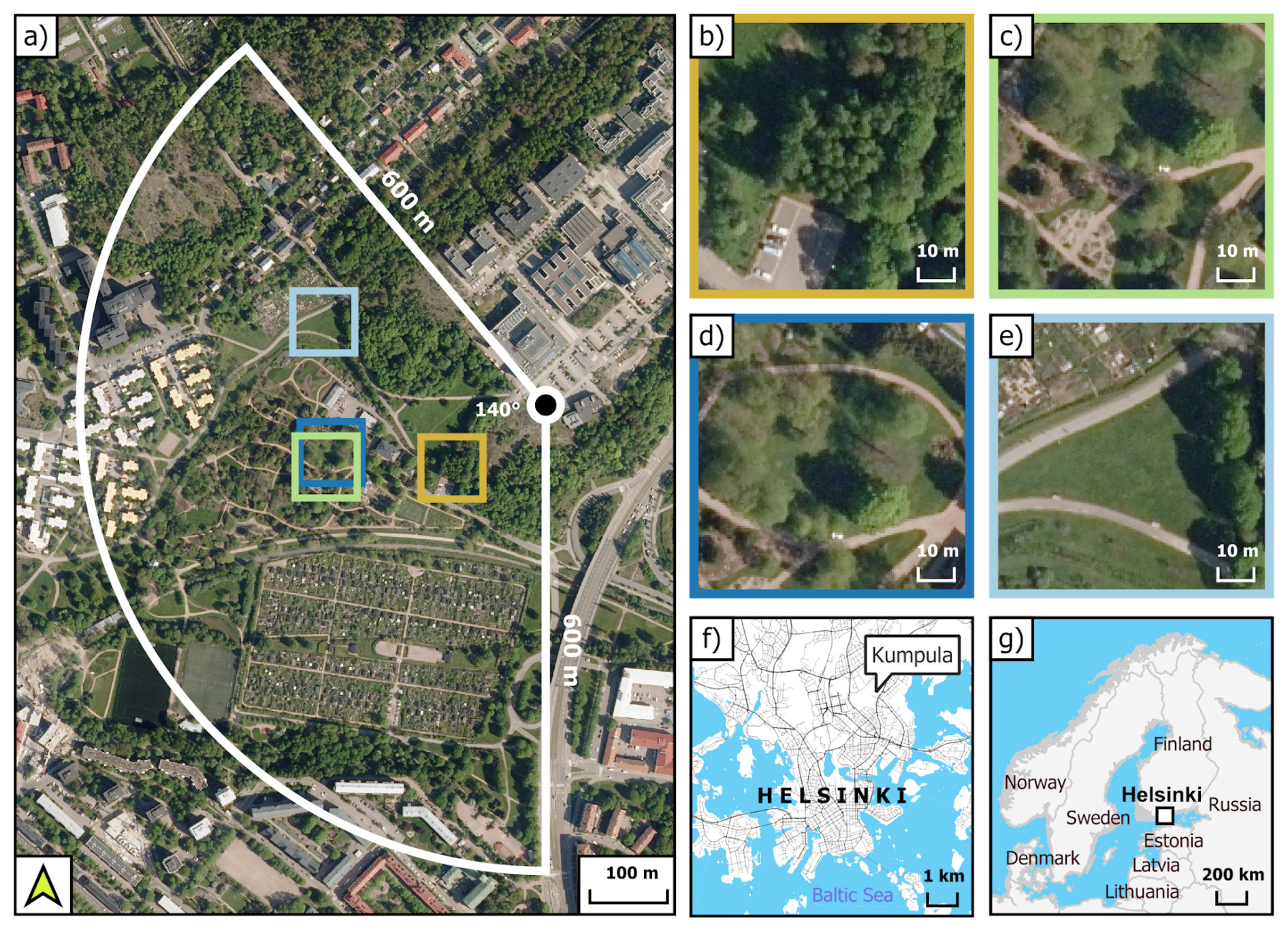
Figure 1 (a) The vegetation types studied (coloured squares) and the modelling target area of this study (white-lined sector), that is, the vegetation sector described in Järvi et al. (2009) that roughly indicates the footprint of the eddy covariance measurements (the tower is represented as a circle). The zoomed images show the different vegetation types studied: urban forest (b), the park with linden trees (c) and irrigated lawn with some non-irrigated patches (d), and the non-irrigated lawn (e). The maps show the location of Kumpula in Helsinki (f) and the locations of Helsinki and Finland (g). Orthophotos by National Land Survey of Finland (2023a), background maps built with the topographic database by National Land Survey of Finland (2023b), and global administrative borders by GADM (2023).

2 Materials and methods

2.1 Study area

The study took place in Kumpula, Helsinki, Southern Finland (60°12^′11.3^′′ N, 24°57^′40.4^′′ E; Fig. 1f, g). The area belongs to the humid continental climate class (Dfb) in the Köppen and Geiger classification (Kottek et al., 2006), as the average temperature exceeds 10 °C from June to September. Helsinki is located on the coast of the Gulf of Finland, which cools the climate in spring and early summer, whereas in autumn and early winter, the sea has a warming effect on the climate. In Helsinki, the mean annual temperature is 6.5 °C, and precipitation is 653 mm (Jokinen et al., 2021).

The study was carried out within a vegetated sector situated southwest of the ICOS (Integrated Carbon Observation System) EC tower FI-Kmp, also known as SMEAR III (Vesala et al., 2008) (Fig. 1a). The study area is a 140° wide sector with a radius of 600 m from the tower. This sector encompasses both the Kumpula Botanic Garden and an allotment garden. It comprises various land cover types: 27 % paved surfaces, 8 % buildings, 27 % tree cover, and 38 % grass surfaces. In 2020–2021, an intensive measurement campaign took place over four sites located within the vegetated sector: a park area with trees and a partly irrigated open lawn, a non-irrigated open lawn, and an urban forest (Fig. 1b–e). Details of the soil properties at the sites are given in Table S1.

The urban forest (60°12^′07.7^′′ N, 24°57^′33.0^′′ E), dominated by silver birches (Betula pendula), is a rather small (25 m×30 m) area located next to the parking area at the eastern side of the Kumpula Botanic Garden (Fig. 1b). Trees were planted around 1990. In 2021, the dominant birches were approx. 23.6 cm in diameter at breast height and 22 m in height. The vegetation was not actively managed, and Aegopodium podagraria prevailed in the ground layer at the site. The soil was classified as sandy loam. The forest was surrounded by an open, managed meadow on its northwestern side and by another forest on the east side with Betula pubescens, Alnus glutinosa, Ulmus glabra, Acer platanoides, and Populus tremula.

The park area (60°12^′08.4^′′' N, 24°57^′21.4^′′ E) in the Kumpula Botanic Garden of the Finnish Museum of Natural History included four linden (Tilia cordata) trees (Fig. 1c, hereafter called park trees) and irrigated lawn (Fig. 1d). The linden trees were originally planted in 1989 and transplanted in 1995 to their current locations close to a gravel footpath. In 2021, the average diameter at breast height was 26.3 cm, and the height was 12.5 m. The ground vegetation below the trees was mowed a few times each year. The ground vegetation was rather diverse, including common grass species (Poa pratensis, Lolium perenne, Festuca sp., Phleum pratense, Dactylis glomerata, and Alopecurus pratensis) and also some more or less rare forbs, such as Cerastium fontanum and Dianthus deltoides.

In the open-lawn area next to the park trees, the vegetation was dominated by Poa pratensis; some other common lawn species including Lolium perenne, Polygonum aviculare, Trifolium repens, and Achillea millefolium were also present. The lawn was fertilized once every few years, most recently in the spring of 2021. An irrigation system with sprinklers was manually regulated to work in conditions that supposedly featured low soil moisture. However, some small patches on the lawn area were also poorly irrigated. Mowing of the lawn was done by a robotic lawnmower, and the grass clippings were shredded and left on the lawn.

Last, the non-irrigated lawn (60°12^′14.0^′′ N, 24°57^′22.2^′′ E) was surrounded by three footpaths 150 m away from the irrigated lawn (Fig. 1e). The eastern side of the lawn was bordered by Acer platanoides, Populus tremula, and Lonicera sp. shrubs. The ground vegetation at this site was dominated by a mixture of Poa pratensis, Lolium perenne, and Festuca sp., coupled with Polygonum aviculare, Trifolium repens, Achillea millefolium, Plantago major, and Taraxacum sp. The soil texture of the non-irrigated lawn was assumed to be the same as that of the park site due to the close distance.

2.2 Models

2.2.1 JSBACH

JSBACH (Reick et al., 2013), the land component of the Earth system models developed by the Max-Planck Institute for Meteorology (Giorgetta et al., 2013), simulates terrestrial energy, hydrology, and carbon fluxes through a suite of submodels. Vegetation is represented by plant functional types (PFT), with this study focusing on the C3 grass and broadleaved deciduous tree PFTs.

Photosynthesis of C3 plants in JSBACH follows the model by Farquhar et al. (1980). The photosynthesis is calculated once to obtain the unstressed canopy conductance, which is then scaled based on the soil moisture in the root zone to obtain the canopy conductance and photosynthesis under water stress. The soil hydrology parameters are set according to soil texture, following Hagemann and Stacke (2014), and the hydrology is simulated using a multilayer soil hydrology scheme.

Seasonal leaf area index (LAI) development is described by the Logistic Growth Phenology (LoGro-P) model (Böttcher et al., 2016). In the case of broadleaved deciduous trees, this development depends on air temperature. The grass phenology additionally incorporates net primary productivity as a determining factor. The maximum LAI was set based on Sentinel-2 data (see Sect. 2.5.1). In addition, the phenology parameters were adjusted to improve the agreement with Sentinel-2 observations regarding the temporal development of LAI. In JSBACH, the photosynthetically active radiation (PAR) in the canopy is described using the two-stream approximation (Dickinson, 1983), which describes the budget of the diffuse radiation in the canopy. The direct radiation is attenuated exponentially in the canopy. Scattering of the direct beam produces diffuse radiation by reflection or transmission.

The dynamics of litter and soil carbon in JSBACH are modelled based on the Yasso soil carbon model (Goll et al., 2015), which features five carbon pools reflecting the chemical quality of organic matter. The model distinguishes between woody and non-woody organic material. The litter pools are further divided into above- and belowground pools. These pools accumulate carbon from litter flux and root exudates. Decomposition transfers carbon between pools and to the atmosphere.

The model was driven with hourly observation-based data of air temperature, precipitation, shortwave and longwave radiation, relative humidity, and wind speed. The simulations include an 8000-year spin-up period to establish the soil carbon pools. The final simulations cover the period from 2005 to 2021. The forest (birch), park (linden), and lawn sites were simulated separately. The park and lawn sites were also simulated with irrigation (see Sect. 2.4).

2.2.2 LPJ-GUESS

The Lund-Potsdam-Jena General Ecosystem Simulator (LPJ-GUESS,  Smith et al., 2001, 2014; Lindeskog et al., 2021) is a process-based dynamic global vegetation terrestrial ecosystem model (DGVM) designed for regional and global studies. It includes a detailed representation of forest ecosystem composition and stand dynamics. It simulates the dynamics and composition of vegetation in response to changes in climate, land use, atmospheric CO₂, and nitrogen. LPJ-GUESS simulates potential vegetation as a mixture of about 20 PFTs, which compete with each other for light, space, and soil resources in each simulated grid cell. Each PFT is characterized by growth form; phenology; photosynthetic pathway (C3 or C4); bioclimatic limits for establishment and survival; and, for woody PFTs, allometry and life history strategy. All individuals of a given age cohort are assumed to be identical (Knorr et al., 2016). Primary production and plant growth follow the approach of LPJ-DGVM (Sitch et al., 2003). The fraction of incoming PAR within the canopy depends on the leaf area index and light reduction via the upper vegetation levels. The plant physiological processes of photosynthesis, respiration, stomatal regulation, and phenological development are simulated at a daily time step within the ecosystem. Soil hydrology and plant water uptake are modelled using a two-layer soil profile. LPJ-GUESS includes dynamic cycling of soil carbon based on the CENTURY model (Parton et al., 1993).

All simulations in this study were initialized with a 500-year spin-up using atmospheric CO₂ concentration from 1901 and repeating detrended ERA5-Land data from 1951 to 1980. The actual simulations covered the years 1901–2021. In this study, separate simulations for each vegetation type were run (forest, non-irrigated park, irrigated park, non-irrigated lawn, and irrigated lawn). The results of the whole vegetated sector were calculated from the separate simulations. In the urban forest simulation, the birches were planted in 1990, and the tree density was set to 5000 trees ha⁻¹. In the park, the sparse linden trees were planted in 1988, and the density was set to 600 trees ha⁻¹. Only C3 grass was set to grow in the lawn simulations. The irrigation rates used in the simulations are introduced in Sect. 2.4.

The LAI calculations in autumn were changed from the standard LPJ-GUESS version. Originally, LAI stayed at its maximum value until the growing season had lasted 210 d. We shortened the growing season length to 190 d to better fit the circumstances in Helsinki and also decreased LAI by 1.5 % (trees) or 2 % (lawn) on days when the daylight hours were less than 14 h and soil temperature was less than 10 °C. Maximum lawn LAI was limited to an average of 2.5 m² m⁻² and the previous year's maximum LAI to simulate the lawn mowing. Also, the LAI of the lawn during dry periods was changed from the LPJ-GUESS standard version to better correspond with the observations. In this study, LAI was decreased by 8 % after running out of water and increased by 8 % after refilling.

2.2.3 SUEWS

The Surface Urban Energy and Water Balance Scheme (SUEWS,  Järvi et al., 2011, 2019) is a neighbourhood-scale urban land surface model used to simulate the urban surface energy, water, and CO₂ balances. The urban surface is separated into seven connected surface types (buildings, paved surfaces, grass, evergreen trees and shrubs, deciduous trees and shrubs, bare soil, and water), with each surface except water having a single soil layer beneath. The urban water balance considers evapotranspiration simulated with the Penman–Monteith equation and modified for urban environments (Grimmond and Oke, 1991), irrigation with either manual or automatic sprinklers, and runoff between the surfaces (Järvi et al., 2011). Canopy conductance is controlled by environmental factors, that is, LAI, solar radiation, air temperature, air humidity, and soil moisture, connecting transpiration to CO₂ uptake estimates; in SUEWS, the maximum potential photosynthesis depends on these environmental limiting factors (Järvi et al., 2019). Respiration is estimated with its exponential relation to air temperature. Both photosynthesis and respiration can be simulated separately for grass and trees; however, the model output is the mean value from the whole simulation domain. In SUEWS, the local 2 m air temperature is simulated by taking into account urban effects (Tang et al., 2021) and is used to estimate photosynthesis and respiration.

The model parameters are based on Järvi et al. (2019). The daily LAI is simulated by accounting for its dependence on growing degree days (GDDs) and senescence degree days (SDDs), both influenced by air temperature. Here, we optimized the leaf-on and leaf-off rates with satellite-based LAI (see Sect. 2.5.1) to expedite the attainment of maximum LAI, while ensuring a more gradual decline during leaf-off. For high latitudes, SUEWS incorporates day length and mean daily temperature as limiting factors for the initiation of senescence. The previously utilized value of 12 h (Järvi et al., 2014) leads to a delay in the onset of leaf-off. Therefore, we adjusted the threshold day length to 14 h (Havu et al., 2024).

As SUEWS is an urban land surface model, the model runs were made only for the whole vegetated sector. The model run was made with an hourly resolution for the whole period of 2005–2021, with 2005 used as a spin-up year. Two different simulations were made to enable comparison between different observational sites: one with irrigation and one without irrigation.

2.3 Driver data

Two sets of hourly driver data were prepared: one for JSBACH and LPJ-GUESS, mainly based on observations near ground level, and another for SUEWS, mainly derived from tower data recorded at 32 m in height. Separate forcing data were used for SUEWS, given its characterization as an urban land surface model designed to simulate local climate conditions utilizing forcing data obtained from the inertial sublayer (Tang et al., 2021).

The first set of driver data included air temperature (2 m), precipitation (1.5 m), shortwave (2 m) and longwave (32 m) radiation, relative humidity (2 m), air pressure (1.5 m), and wind speed (10 m). The primary data source was observations from the Kumpula weather observation station (60°12^′11.1^′′ N, 24°57^′40.7^′′ E) operated by the Finnish Meteorological Institute (FMI, 2022). Data gaps were filled using observations from the urban measurement station SMEAR III, which is located next to the weather station (Järvi et al., 2009; SMEARIII, 2022). The second set of driver data included air temperature, shortwave and longwave radiation, and wind speed from the SMEAR III measurement tower at 32 m in height, alongside precipitation, relative humidity, and air pressure from the nearby rooftop at 26 m. Both observational datasets were gap-filled using hourly ERA5-Land data (Muñoz Sabater et al., 2021; Muñoz Sabater, 2019). ERA5-Land data were used from 1951 to 2004. The data for model spin-up in the years 1900 to 1950 were randomly generated based upon the years from 1951 to 1980.

Figure 2 Observed daily temperature and monthly precipitation in Kumpula during 2018–2021.

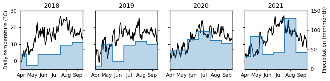
The performance of the models was evaluated during two study periods. The primary and most intensive one covered the years 2018–2021, during which 2018 exhibited the highest temperatures and the least precipitation, while the subsequent years were more similar to each other (Fig. 2). According to the driver data, the growing degree days to base 5 °C (GDD5) for the years 2018, 2019, 2020, and 2021 were 1964, 1679, 1720, and 1777 °C, respectively. The accumulated precipitation during the irrigation period (May–August) was 144, 215, 296, and 293 mm for the corresponding years. The secondary study period was longer, covering the years 2006–2021 (Fig. S1 in the Supplement). During this period, 2017 had the lowest and 2018 the highest GDD5, and they showed the respective lowest and highest maximum temperatures (Table S2 in the Supplement). The years 2006 and 2011 also had GDD5 above 1800 °C. The years 2006 and 2018 had the lowest amounts of summertime precipitation and the highest number of dry days (Table S2), whereas 2007 and 2009 had over 30 % more rainfall than average during summertime.

2.4 Irrigation

The irrigation scheme in SUEWS (Järvi et al., 2011) considers both automatic and manual irrigation on an hourly scale, as they tend to differ in their timing and response to weather conditions. The daily water use (I_e; mm d⁻¹) is estimated from mean daily air temperature (T_d) and time since rain (t_r; d):

$$\begin{array}{}\text{(1)}& I_e=b_{\mathrm{0}}+b_{\mathrm{1}}{T}_{\mathrm{d}}+b_{\mathrm{2}}{t}_{\mathrm{r}},\end{array}$$

where b₀,b₁, and b₂ are site-specific coefficients. The daily precipitation is then divided by the fraction of irrigated surfaces for each surface type specified in the model input files separately. The timing of the start and end of the irrigation season needs to be specified. For Helsinki, the irrigation season has been specified to start at the beginning of June and continue until the end of August. The site-specific coefficients b₀,b₁, and b₂ for Kumpula are −5.8 mm, 0.7 mm K⁻¹, and 0.2 mm d⁻¹, respectively (Järvi et al., 2017).

Table 1 Total water consumption between June and August as reported by the Kumpula Botanical Garden and the corresponding estimate of daily average irrigation [mm d⁻¹]. The irrigation estimate based on an algorithm accounting for both temperature and precipitation is given in the last column.

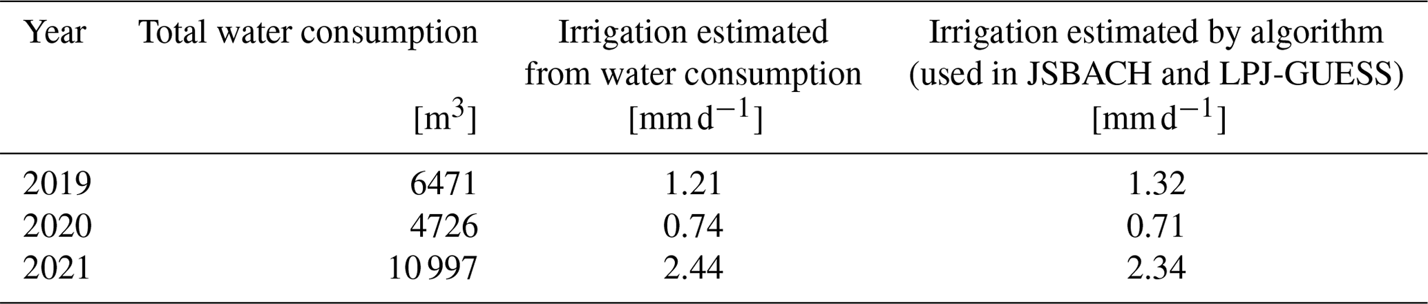
There is no irrigation scheme in JSBACH and LPJ-GUESS; therefore the irrigation was included as extra precipitation during the summer months. The daily average irrigation for the irrigated areas in the vegetation sector studied was estimated from June to August water consumption data obtained from the Kumpula Botanic Garden. Water consumption data were available for 2019–2021 (Table 1). It was estimated that 2000 m³ of water was used annually to maintain a pond in the garden, and this amount was removed from the total consumption. The area of the garden is 6 ha, and we assumed that just two-thirds of this area was irrigated, excluding, for example, maintenance and forested areas. Based on these assumptions, we estimated the daily average irrigation from June to August to be 1.21, 0.74, and 2.44 mm d⁻¹ in 2019, 2020, and 2021, respectively (Table 1). In order to extend the irrigation data to the whole simulated period of 2005–2021, we used an algorithm that considered both temperature and precipitation. We used 2-week running means; if the average temperature over 2 weeks was above 19 °C (hot) or if the average precipitation was below 1.4 mm d⁻¹ (dry), then the irrigation was 1.7 mm d⁻¹. The extra precipitation was added to the hourly forcing data between 08:00 and 16:00 LT (local standard time). If it was both dry and hot over 2 weeks, then the irrigation was increased to 5.0 mm d⁻¹. In this case, the excess precipitation was added to all hours of the day. The algorithm produced year-to-year variation similar to that estimated from the garden water consumption data (Table 1). In the simulations with JSBACH and LPJ-GUESS, irrigation was added to the precipitation between June and August.

The irrigated area within the sector was estimated by assuming that two-thirds of both the Kumpula Botanic Garden and the allotment garden was irrigated, while areas outside of these gardens were not irrigated. As a result, we assumed that 28 % of the trees and 42 % of the grass areas (lawns) were irrigated in this sector.

2.5 Observations

2.5.1 Leaf area index

The four intensive sites were monitored using remote sensing imagery from the European Space Agency (ESA) Sentinel-2 satellites during 2018–2021. Atmospherically corrected Level-2A (L2A) Sentinel-2 multispectral data were retrieved using the Google Earth engine (GEE; https://earthengine.google.com/, last access: 15 March 2024) cloud data platform. The scene classification band available in L2A products was used to filter away image acquisition dates during which the field was covered by snow, cloud, or cloud shadow. From the Sentinel-2 data, we calculated the leaf area index estimated using the ESA Sentinel Application Platform (SNAP) Biophysical Processor neural network algorithm (Weiss and Baret, 2016; Nevalainen et al., 2022). The uncertainty calculations are described in detail by Nevalainen et al. (2022).

2.5.2 Photosynthesis

Light responses of net ecosystem exchange of CO₂ (NEE) of the partly irrigated lawn (Fig. 1d) were determined by manual chamber measurements conducted at four fixed plots (60 cm×60 cm) every second week from June to September in 2021 and 2022. More infrequent measurements were also conducted in May and from October to December. The setup consisted of a transparent chamber attached to a CO₂ and H₂O analyser (Li-840A, LI-COR, Inc., Nebraska, USA), air temperature and humidity sensor (BME280, Bosch Sensortec GmbH, Reutlingen, Germany), and photosynthetically active radiation (PAR) sensor (PQS1, Kipp & Zonen, Delft, Netherlands). Details of the setup, the full protocol, flux calculations, and the light response curve fitting are described in Trémeau et al. (2024). Photosynthesis (gross primary production, GPP) was estimated for each 30 min period utilizing automatically recorded mean PAR at SMEAR III and the estimated light response curves, assuming that (1) NEE at zero light represents total ecosystem respiration (TER), (2) TER was independent of the light intensity during the chamber measurements, and (3) GPP = TER-NEE. Daily GPP was obtained by summing up the GPPs estimated for each 30 min period. Even though the lawn area was mainly irrigated, it also included small, inadequately irrigated patches, which allowed us to divide the observations into adequately and poorly irrigated ones.

In the park, CO₂ exchange of three separate linden shoots was measured with an automatic chamber system operating continuously at the site from June to September in 2020–2021. The chambers were mostly open, enabling natural radiation and precipitation conditions. They closed automatically two times per hour for 2 min at a time, resulting in 48 exchange rates per chamber in 1 d in naturally varying environmental conditions. The setup at each shoot consisted of a transparent chamber of approximately 1 L, sample tubing, a CO₂ analyser (GMP343, Vaisala Oyj, Vantaa, Finland), a fan mixing the air, PAR (SQ-420X Smart Quantum Sensor, Apogee, Logan, USA), relative humidity and temperature (HygroClip 2 HC2A, Rotronic AG, Bassersdorf, Switzerland) sensors, and a pump that circulated sample air from the chamber to the analyser and back in a closed loop. The CO₂ exchange was calculated from the rate of change in the CO₂ concentration during the closure. A simple light response curve was fitted to these exchange rates. Since the specific placement of the chambers may not have accurately reflected the typical light conditions experienced by all leaves, we assessed instantaneous photosynthesis under unshaded conditions resembling those found in the uppermost canopy. This was achieved by utilizing the light response curve and photosynthetically active radiation (PAR) measurements obtained at the SMEAR III site. Daily photosynthesis was then calculated by summing the instantaneous rates, as described previously.

In addition to the automatic measurements conducted on the lindens, the light responses of CO₂ exchange of tree leaves were manually measured using a portable gas exchange system (Walz GFS-3000, Heinz Walz GmbH, Germany) with a standard measuring head (2 cm×4 cm) on the trees in the park and in the urban forest during the summers of 2020 and 2021 at approximately 4-week intervals. During each measurement, the CO₂ concentration was set to a fixed value of 415 ppm, representing the typical daytime CO₂ concentration in the area, but the temperature was not set to any value and followed the ambient conditions. The measurement included different light intensities, changing automatically from 1500 down to 0 $\mathrm{\mu }\mathrm{mol}{\mathrm{m}}^{-\mathrm{2}}{\mathrm{s}}^{-\mathrm{1}}$ over 43 min. The measurements were performed on a single healthy leaf at two or three heights in three individual trees in the forest and at linden sites on the southern or southwestern side of each tree. As a result, the linden site included altogether nine light responses (three Tilia cordata trees, three heights) and the forest site six (three Betula pendula trees, two heights) during each repetition. The details of the measurement protocol and fitting of the light response curve are described in detail by Ahongshangbam et al. (2023a). Again, daily photosynthesis during the measurement days was derived utilizing the light response curves and the automatic PAR measurements at SMEAR III.

2.5.3 Soil respiration

The soil respiration CO₂ flux was measured using manual chamber measurements in both the park (under the park trees) and the urban forest in 2020–2021. The measurements were conducted weekly in May–September and fortnightly or monthly in October–December. The measurement setup consisted of a small opaque chamber (volume =0.007434 m³) equipped with a CO₂ probe (GMP343, Vaisala Oyj), relative humidity and temperature sensor (HMP75, Vaisala Oyj), and a small battery-powered fan to ensure air circulation within the chamber. Measurement data from the sensors were stored on-site in a handheld reading console (MI70, Vaisala Oyj). Eight steel frames were inserted a couple of centimetres into the soil at both measurement sites, and the measurement chamber was placed on top of each of the frames for 4–5 min while measuring the CO₂ concentration, relative humidity, and air temperature change inside the chamber. The soil respiration CO₂ flux was calculated from the rate of change in the CO₂ concentration during the closure. The chamber system is described in detail by Pumpanen et al. (2015) and Karvinen et al. (2024) and the measurement point selection and flux calculation by Karvinen et al. (2024).

2.5.4 Soil moisture and temperature

Soil moisture was measured manually with a soil profile probe (PR2 (SDI-12), Delta-T Devices, Cambridge, UK) and a handheld reading console (HH2, Delta-T Devices) in both the park and the urban forest. Six fibreglass access tubes (ATS1, Delta-T Devices) were installed in the soil in 2020 and measured weekly during the main growing season in 2020–2022. The profile probe measures soil moisture at depths of 10, 20, 30, and 40 cm. Manual soil temperature measurements were conducted with a handheld console setup (Pt100 and HH376, Omega Engineering Inc., Connecticut, USA) together with all manual chamber measurements.

2.5.5 Sap flow

Sap flow measurements were conducted using a thermal dissipation probe (TDP; Granier, 1985) consisting of two thermocouple needles (20–30 mm long), where one needle acts as a heating probe and the other as a reference probe. The sap flow density is calculated from the temperature difference between the heated probe and the reference probe. We measured three dominant trees at a height of 1.3 m at the park site and at 2.0 m at the forest site, with a vertical distance of 10 cm between the heated and the reference probes. The setup, flow calculations, and data are described in detail in Ahongshangbam et al. (2023a). First, we compared the sap flow rates and the model estimates of transpiration to analyse seasonal dynamics. Second, the sap flow rates were transformed into estimates of whole-tree transpiration by multiplying the rates by species-specific values for sapwood area from the literature, namely 349.7 cm² for the birches (Zapater et al., 2013) and 433.8 cm² for park trees (Leuzinger et al., 2010).

2.5.6 NEE from eddy covariance

The net ecosystem exchange (NEE) was estimated from the eddy covariance measurements located at the SMEAR III station (Vesala et al., 2008; Järvi et al., 2009). The source area of the 31 m measurement tower varies depending on the meteorological conditions, as the fetch can be larger during stable winter conditions (up to 1 km). Southwest of the tower (180–320°) lies the Kumpula Botanic Garden and allotment gardens (the vegetation sector), where the closest road is located 800 m from the mast.

The wind components were measured with an ultrasonic anemometer (USA-1, Metek GmbH, Germany) and the CO₂ mixing ratios with two infrared gas analysers (closed-path analyser LI-7000 or open-path analyser LI-7500; LI-COR, Lincoln, NE, USA), depending on the year, as the open-path analyser was installed in 2005 and the closed-path one in 2014. The 60 min flux values were calculated following Nordbo et al. (2012). The period analysed started in 2006 and ended in 2021. Measurements coming from the vegetation sector based on wind direction were used in order to limit emissions from the road located east of the tower. As flux values are 60 min averages from the 10 Hz data, some traffic-related emissions might still be included in the estimation, as well as emissions from human metabolism. The daily values of NEE were calculated from the vegetation sector, with complete data coverage for a full day available for only 15 % of the days. Consequently, when individual data gaps were shorter than 4 h, they were filled using linear interpolation. This process resulted in an increase in data coverage to 25 % over the 16-year period.

2.6 Evaluation statistics

The assessment of model performance involves the utilization of standard statistical metrics, including a Pearson correlation coefficient (r) and the mean bias error (MBE). A scientific colour map is used in this study to prevent visual distortion of the data and exclusion of readers with colour-vision deficiencies (Crameri et al., 2020).

Table 2 Mean Pearson's correlation coefficients between observations and the model estimates. The correlations for sap flow were determined for 2021; leaf area index (LAI) for 2018–2021; soil temperature, soil moisture, leaf-based photosynthesis (GPP), and soil respiration for 2020–2021; and net ecosystem exchange of CO₂ (NEE) in the target area (Fig. 1a) for 2006–2021.

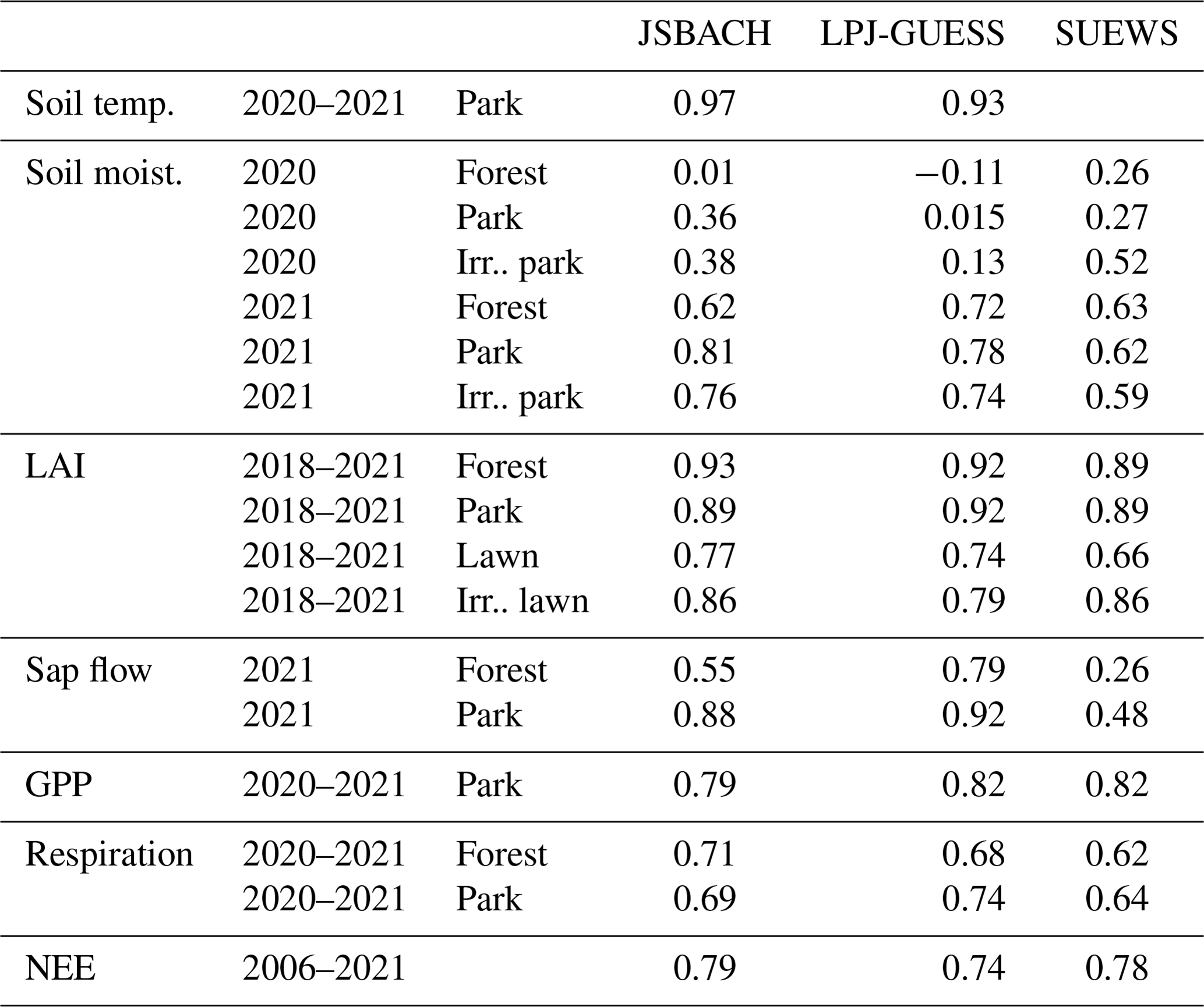
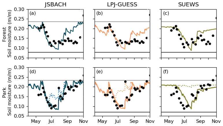
Figure 3 Daily mean soil moisture of the root zone estimated by the different models (lines) and observations (dots) in the urban birch forest (a, b, c) and the park site with trees (d, e, f) from May to October 2021. Solid lines are from non-irrigated simulations and dotted lines from irrigated ones. The horizontal black lines represent the wilting points used, and the grey lines are the field capacities. The soil moisture was simulated for each model for the specific root zones.

3 Results

3.1 Soil conditions

JSBACH and LPJ-GUESS displayed a rather consistent pattern when simulating root zone temperature, following the observations closely in both the forest (not shown) and the park trees (Fig. S2). The Pearson's correlation coefficients of soil temperature ranged between 0.93 and 0.97 for these models (Table 2). SUEWS does not simulate soil temperature and consequently was excluded from the comparison.

All models exhibited similar predictions for soil moisture dynamics within the root zone in the urban forest and park sites for 2021 (Fig. 3). However, it is noteworthy that the soil volume represented varies in the different models. For instance, JSBACH considered a root depth of 0.45 m for park trees (linden) and 0.65 m for forest trees (birch). LPJ-GUESS accounted for the soil moisture of the root zone, with 60 % of birch (forest) roots in the uppermost 0.5 m and 40 % in the next 1 m layer, with 80 % and 20 % for the park trees (linden). In contrast, SUEWS simulated soil moisture across the whole simulation domain from an average depth of 11–35 cm, depending on the surface type, resulting in no differentiation between vegetation types. The soil hydraulic properties (wilting point and field capacity) are calculated using the Cosby et al. (1984) regression relationships from the soil sand, silt, and clay fractions at the measurement sites.

The simulations generally supported the observed soil moisture dynamics in the early season. However, in the latter half of the 2021 season, the observed soil moisture in the forest did not increase as rapidly as the simulations predicted (Fig. 3a–c). The Pearson's correlation coefficients were 0.62–0.81 for JSBACH, 0.72–0.78 for LPJ-GUESS, and 0.59–0.63 for SUEWS (Table 2). Soil moisture in the urban forest and park sites for 2020 is shown in Fig. S3. The soil was moister in 2020 than in 2021, and the soil was moist until late autumn, while all the models predicted drier soil, resulting in lower correlations: 0.01–0.38 for JSBACH, −0.11–0.13 for LPJ-GUESS, and 0.26–0.52 for SUEWS. The extent to which simulated soil moisture increased due to irrigation varied between the models, with the smallest change observed in JSBACH (Fig. 3e) and the most significant in SUEWS (Fig. 3f), which employs its own irrigation scheme. For each model, a value according to its root zone was calculated from the soil moisture observations.

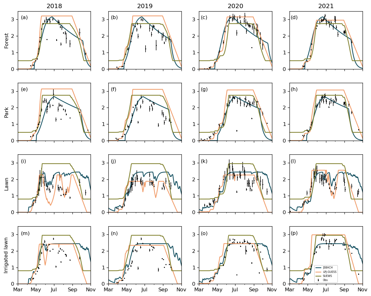
Figure 4 Daily one-sided leaf area index (LAI) simulated by JSBACH (blue), LPJ-GUESS (orange), and SUEWS (green) and satellite observations (dots) of the studied vegetation types in 2018–2021. The error bars of the observations represent the standard deviations.

3.2 Leaf area index (LAI)

All models effectively captured LAI dynamics when compared against satellite observations from 2018 to 2021 (Fig. 4). They reasonably predicted the timing and magnitude of the LAI increment in the different vegetation types studied during spring. In midseason, LPJ-GUESS and SUEWS generally maintained stable LAI values for trees, whereas JSBACH exhibited a decrease similar to the observations (Fig. 4a–h) due to a small shedding rate applied during the vegetative phase. LAI of lawns exhibited variation based on dry seasons and possible irrigation levels. In dry conditions, the net primary production (NPP) in JSBACH is limited by decreasing soil moisture, and LAI is decreased. However, low soil moisture does not decrease LAI in SUEWS; therefore, simulated LAI remained constant for both non-irrigated and irrigated lawns. In contrast, JSBACH and LPJ-GUESS responded to drying conditions in non-irrigated lawns, while the irrigated lawns showed LAI stability across all models (Fig. 4i and l).

Pearson's correlation coefficients indicated differences in model performance for LAI (Table 2). On average, the highest correlation was observed for JSBACH in the urban forest (0.93), for LPJ-GUESS in the park (0.92), for SUEWS and JSBACH for the lawn (0.86), and for JSBACH for the non-irrigated lawn (0.77) (Table 2). Additionally, the mean bias error (MBE) (Table S3) displayed variability between the models. On average, the smallest MBE was associated with JSBACH for the forest (0.03), park (−0.01), and irrigated lawns (0.27), whereas LPJ-GUESS exhibited the lowest MBE for the non-irrigated lawns (−0.01).

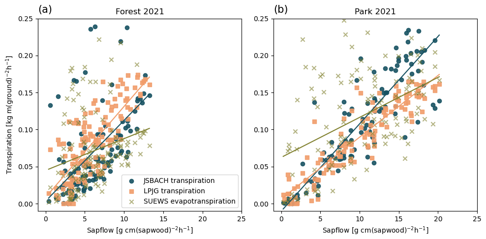
Figure 5 Correlation between daily mean sap flow measurements and the modelled transpiration by JSBACH (blue circles), LPJ-GUESS (orange squares), and SUEWS (green crosses) (a) in the urban forest and (b) in the park site in 2021. The measurements are averages over three trees. Note the different units for simulations and observations.

3.3 Transpiration

Figure 5 shows the correlation of modelled transpiration (from JSBACH and LPJ-GUESS) or evapotranspiration (from SUEWS) and the sap flow measurements. The correlation coefficient (Table 2) revealed the best agreement for LPJ-GUESS, with r values of 0.79 for the forest site and 0.92 for the park site. JSBACH also demonstrated good agreement with observations, with r values of 0.55 for the forest site and 0.88 for the park site. In contrast, SUEWS had lower correlation coefficients, primarily due to the challenge of comparing evapotranspiration instead of transpiration, resulting in values of 0.26 for the forest site and 0.48 for the park site. The comparison between simulated transpiration and sap flow observations was difficult due to the differences in the units: models simulated transpiration of the whole canopy per ground area, whereas the observations described the sap flow rate per sapwood area. Thus, the correlation coefficients indicate the similarity of seasonal dynamics between models and observations. The modelled tree-scale estimates for transpiration were on the lower end of the range of the sap-flow-based estimate for transpiration when the sap flow rate was multiplied by the literature values for the sapwood areas (Fig. S5).

Based on observations, sap flow rates in the urban forest site were lower than those in the park, as irrigation increased the water availability. Consequently, JSBACH simulated larger transpiration rates for the park than for the urban forest, while LPJ-GUESS maintained transpiration within a similar range in both environments. JSBACH estimated smaller transpiration rates compared to LPJ-GUESS in the urban forest, whereas at the park site, JSBACH estimated larger transpiration rates. However, as SUEWS simulates evapotranspiration across the whole simulation domain, encompassing both trees and grasses, direct comparisons of sap flow observations and other models posed challenges. As a result, SUEWS exhibited larger variability and scatter, which was particularly evident at the park site. During peak observation periods, SUEWS estimated lower values for the urban forest compared to other models, while in the park, they fell between the estimates from JSBACH and LPJ-GUESS.

Simulated transpiration varied among the models, which was particularly evident at the forest site from May to June. At the forest site, SUEWS predicted the lowest rates, while JSBACH predicted the highest values, at least for a few weeks (Fig. S4a). Daily and seasonal variations simulated by JSBACH and LPJ-GUESS closely matched observations during the second half of the growing period, although they showed clear overestimation in early summer. For the park trees, the annual pattern and day-to-day changes simulated by LPJ-GUESS and JSBACH closely resembled the observations in 2021 (Fig. S4b). Furthermore, the higher evapotranspiration by SUEWS compared to the other models coincided with rainy days, indicating that a substantial proportion of the evapotranspiration was attributed to evaporation rather than transpiration (not shown).

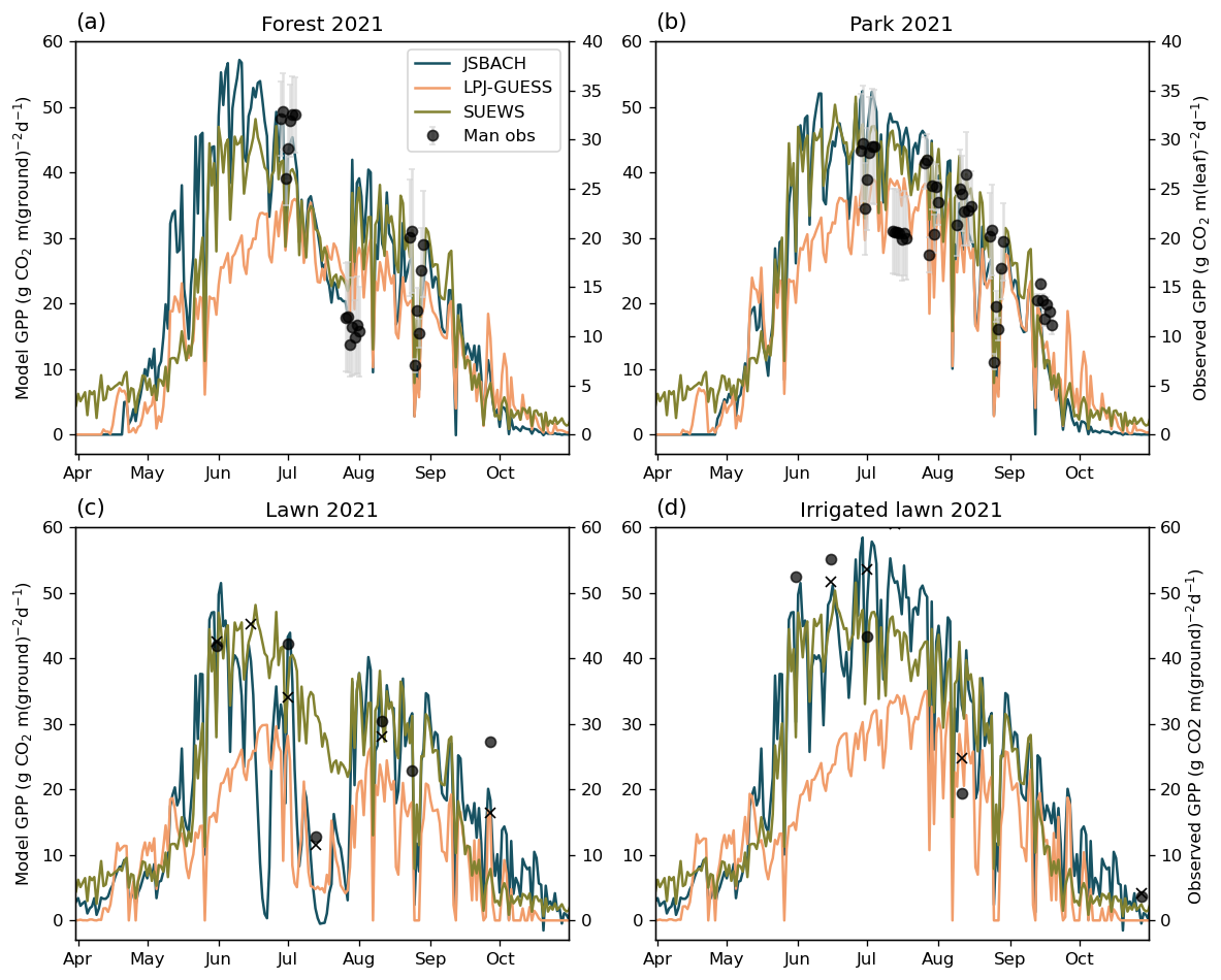
Figure 6 Modelled daily photosynthesis (GPP) per ground area and measurement-based leaf-scale estimates of daily photosynthesis in the birch forest (a), the park with linden trees (b), the non-irrigated lawn (c), and the irrigated lawn  (d) in the year 2021. In (a) and (b) observations (dots) are averages estimated from the light response curves derived from nine measurements collected from three different trees. Error bars represent standard deviations of the averages. In (c) and (d) dots and crosses show individual observations. Note the different units for simulations and observations of forest and park sites.

3.4 Photosynthesis (GPP)

All model simulations for GPP followed the seasonal dynamics of the daily GPP estimations derived from the manual observations of the forest, park, and lawn sites in 2021 (Fig. 6). However, the simulations were per tree-covered land area and observations were mainly per sunlit leaf area, making the comparison of actual magnitudes challenging. GPP by LPJ-GUESS was lower than that of JSBACH and SUEWS for all studied vegetation types, especially in the early season (Fig. 6). JSBACH, LPJ-GUESS, and SUEWS reproduced the observed decrease in GPP during the dry conditions in the urban forest in July 2021 (Fig. 6a). Compared to other models, SUEWS operates differently. While other models simulate different vegetation types separately (urban forest, park, irrigated lawn, and non-irrigated lawn), SUEWS conducts simulations based on the whole vegetation sector, and only two separate simulations, a non-irrigated and an irrigated, were run. The non-irrigated simulation of SUEWS was used to represent the GPP of non-irrigated lawns and urban forests, while the irrigated simulation was used for parks and irrigated lawns. However, the daily rates in SUEWS were fairly similar to those in JSBACH for all studied vegetation types.

At the poorly irrigated lawn plots, the observed GPP decreased during the dry period in July 2021, which JSBACH, LPJ-GUESS, and SUEWS were able to reproduce (Fig. 6c). Although SUEWS also reproduced the impact of the dry period on GPP, it exhibited a much smaller reduction, maintaining relatively higher GPP levels during the dry period. On the adequately irrigated lawn plots, such midsummer suppression was neither observed nor estimated (Fig. 6d), and the modelled GPP was generally higher than at non-irrigated sites. In July 2021, the GPP of the non-irrigated sites was about 30 % of the irrigated ones in JSBACH and LPJ-GUESS and about 70 % of that in SUEWS. For both types of lawns, JSBACH and SUEWS simulated the highest daily rates of photosynthesis and LPJ-GUESS the lowest (Fig. 6).

The GPP derived from the automatic measurements of the park trees provided further support for the ability of the models to simulate seasonal dynamics in GPP. All models were able to estimate the autumn senescence in daily GPP observed by the automatic chambers in the park in 2020 (Fig. S6a), resulting in a high correlation (between 0.89 and 0.91; Fig. S7a). In 2021, the models overestimated the early-season GPP (Fig. S6b), which caused lowered r values of 0.68–0.76 (Fig. S7b), even though in the latter half of the season, the temporal dynamics were again similar between models and observations (Fig. S6b). LPJ-GUESS and SUEWS showed the highest 2-year average r values (0.82; Table 2).

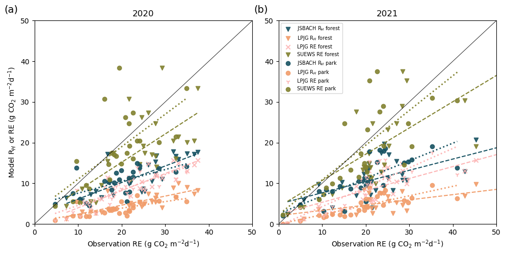
Figure 7 Correlation between daily mean soil respiration (RE) from observations and simulated RE or heterotrophic respiration (R_H) from the different models for the park tree and urban forest sites in 2020 (a) and 2021 (b). Modelled values are R_H from JSBACH and LPJ-GUESS and RE from SUEWS and LPJ-GUESS. Observations are means of manual observations from eight collars. Dashed lines show the fit between modelled and observed non-irrigated forested sites. Dotted lines are the fits between irrigated park site simulations and observations. SUEWS results are from the irrigated simulation.

3.5 Soil respiration

The models displayed reasonably high correlations with mean daily observations of soil respiration under park trees and the urban forest (Table 2). JSBACH simulated heterotrophic respiration (R_H); thus we examined R_H in both JSBACH and LPJ-GUESS to compare the models and RE from LPJ-GUESS and SUEWS. R_H comparison resulted in a difference in the levels between simulated R_H and modelled soil respiration (RE; Fig. 7), but the seasonal dynamics aligned well (Figs. S8 and S9). The R_H modelled by JSBACH was about half that of the observed soil respiration, while LPJ-GUESS seemed very low (Figs. 7, S8 and S9).

JSBACH, in particular, demonstrated a reasonable correlation with observations at both the forest and park sites, achieving r values of 0.69–0.71 (Table 2). Figure 7 shows that JSBACH simulates comparable R_H values for both non-irrigated forest and irrigated park trees in both years. However, simulations showed variations between years. In 2021, a dry year, both sites exhibited lower respiration values compared to 2020, a normal year. Both sites and years aligned quite well with observations: in 2020, r values were 0.63 for park and 0.77 for forest. However, in 2021, the results were in the opposite order: the irrigated simulation resulted in an r value of 0.76, while the non-irrigated simulation performed worse, with a lower r value of 0.65. In contrast, LPJ-GUESS simulated the lowest respiration values among all the models but maintained reasonable r values of 0.68 for non-irrigated and 0.74 for irrigated trees, in the case of R_H (Table 2), and better r values of 0.84 for non-irrigated and 0.80 for irrigated trees, in the case of RE. It underestimated soil respiration during both years (Fig. S8). In Fig. 7, it can be seen that modelled R_H is of the same magnitude for both sites, especially in 2020. The difference between years was also small in the LPJ-GUESS simulations. In 2020, SUEWS provided reasonable estimates, with r values of 0.65 and 0.66, but its performance in 2021 was not as good, as it tended to overestimate soil respiration during the summer, resulting in slightly lower r values of 0.59 and 0.63.

The analysis revealed seasonal variations and the influence of dry conditions on respiration across the forest and park sites. The JSBACH and LPJ-GUESS models depicted a reduction in respiration during dry periods (Fig. S8). At the same time, SUEWS showed similar soil respiration values to the irrigated simulation by JSBACH during dry periods in 2021 (Fig. S9). Examining ecosystem respiration across different simulations revealed that SUEWS cannot consider the impact of soil moisture on respiration, unlike the other models. This suggests that SUEWS, initially designed for irrigated low vegetation, may overestimate respiration when applied to non-irrigated lawns.

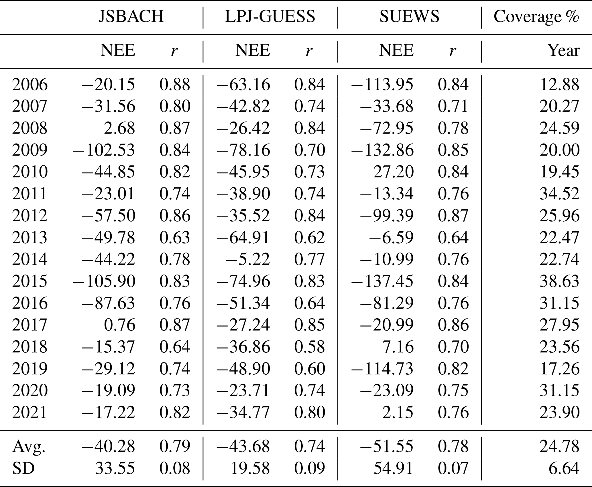
Table 3 Yearly net ecosystem exchange (NEE; g C m⁻²) and Pearson's correlation coefficients between observed and simulated NEE from different models over the diverse urban area (Fig. 1a) and observation data coverage during the year (%) in different years. Negative NEE values indicate a sink of carbon.

Figure 8 Measured (dots) and modelled daily mean net ecosystem exchange (NEE; g C m⁻²) of the target area (Fig. 1) during summer months (May–September) from 2007 to 2021. Panel (p) shows the average over 2006–2021.

3.6 Net ecosystem exchange (NEE) over the vegetation sector

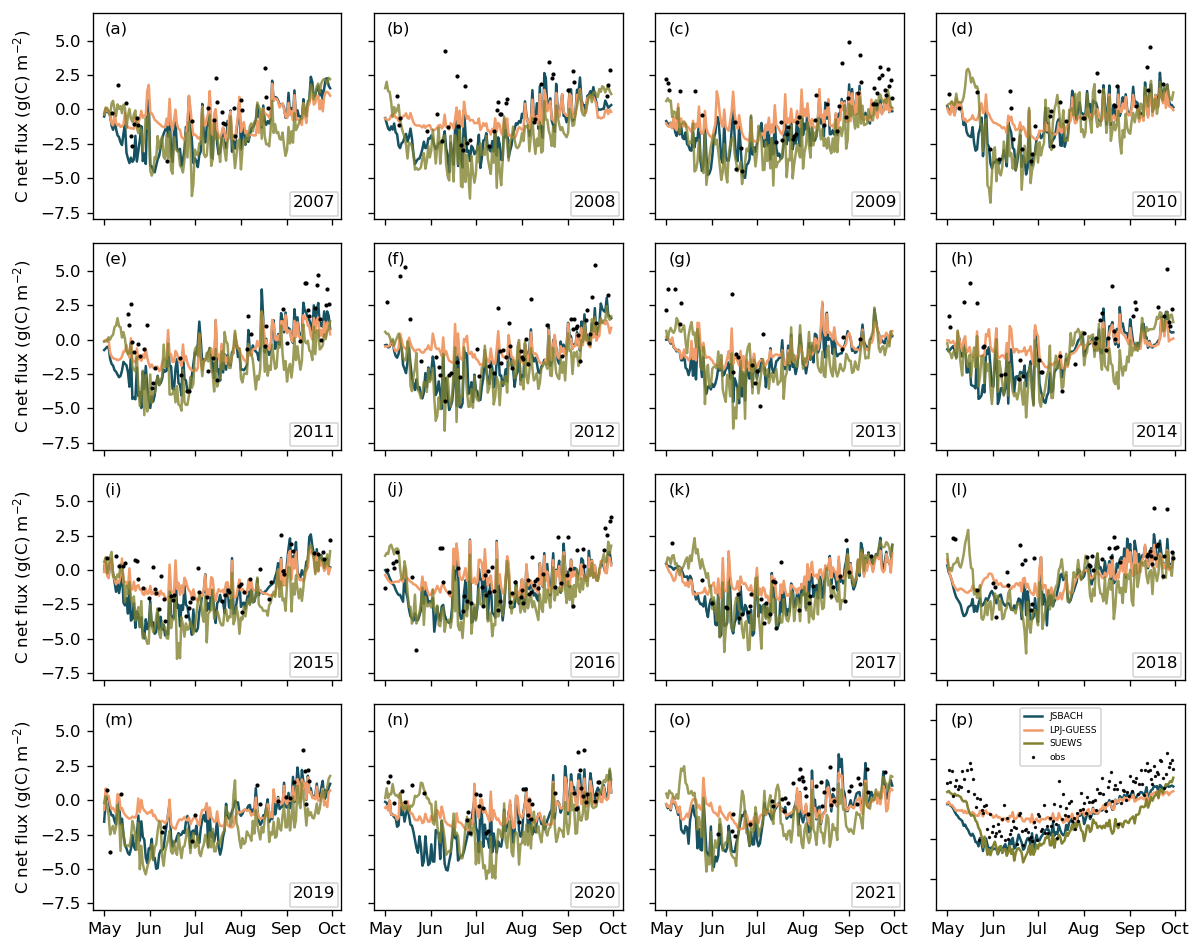
Each vegetation type was simulated separately by JSBACH and LPJ-GUESS, and the NEE of the vegetation sector (Fig. 1a) was calculated from these separate NEEs. SUEWS simulated the NEE sector. The simulated results were compared to the estimate of NEE derived from EC measurements. Evaluation of model performance was particularly complicated during the spring recovery due to low measurement coverage (Figs. 8, S10, Table 3).

Additionally, the comparison was further complicated by the uncertain amount of anthropogenic emissions consistently observed. On average, SUEWS estimated the anthropogenic emissions to be around 0.84 $\mathrm{g}\mathrm{C}{\mathrm{m}}^{-\mathrm{2}}{\mathrm{d}}^{-\mathrm{1}}$ (Järvi et al., 2019). Nevertheless, the models were able to roughly simulate the observed range of the daily and seasonal dynamics in the summertime NEE across the study area (Fig. 8). The correlation coefficients between the EC measurements and the different models averaged between 0.74 and 0.79 (Table 2), varying across different years between 0.63 and 0.88, 0.58 and 0.85, and 0.64 and 0.87 for JSBACH, LPJ-GUESS, and SUEWS, respectively (Table 3).

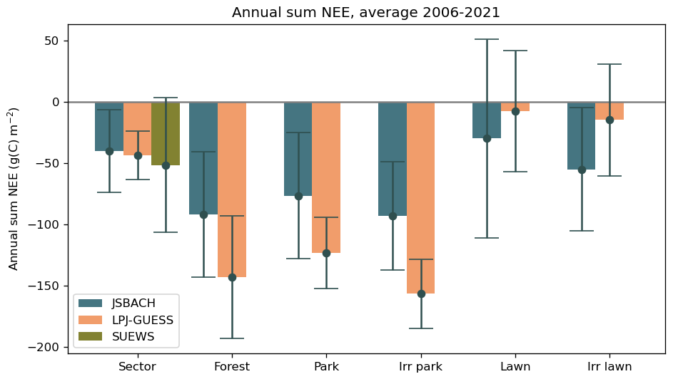
Figure 9 Mean annual carbon sequestration (NEE) in the study area (Fig. 1a) and for the separate vegetation types in the different models over 2006–2021. The error bars represent the standard deviations over the years.

The models displayed varying seasonal patterns in NEE (Fig. S10). On average, SUEWS simulated the highest emissions during the winter and the most substantial sinks during the summer, while the lowest fluxes during both seasons were observed in simulations by LPJ-GUESS. It simulated less seasonal variation in NEE than was observed (Fig. S10a). When comparing all the models, the midsummer sink was the lowest in LPJ-GUESS (Fig. 8), but the annual sinks over the target area were similar in all the models (Fig. 9). Nevertheless, the r values for the years 2006–2021 were nearly as high as those for JSBACH and SUEWS (Table 3). Throughout the growing season (Fig. 8), JSBACH and SUEWS provided comparable NEE estimates, although some differences were noticeable. In 2010 and 2020, JSBACH indicated an earlier sink, whereas SUEWS tended to produce larger sinks during autumn compared to EC observations. One of the most prominent distinctions between the models was related to their wintertime (October–April) NEE estimations, with average winter sum values of 160, 61, and 205 $\mathrm{g}\mathrm{C}{\mathrm{m}}^{-\mathrm{2}}{\mathrm{yr}}^{-\mathrm{1}}$ for JSBACH, LPJ-GUESS, and SUEWS, respectively (not shown).

From 2006 to 2021, the models demonstrated pronounced annual variation in NEE across the vegetation sector. The average NEE values were −40 (±34), −44 (±19), and −52 (±55) g C m⁻² for JSBACH, LPJ-GUESS, and SUEWS, respectively (Table 3). For the majority of years, the models estimated that the vegetation sector acted as a carbon sink. However, there were a few exceptions. In 2008 and 2017, JSBACH indicated that the sector could act as a small carbon source (2.7 and 0.76 g C m⁻²), while SUEWS suggested that in 2010 (27 g C m⁻²), 2018 (7.2 g C m⁻²), and 2021 (2.2 g C m⁻²), the sector could function as a source. The positive values are small, except for SUEWS in 2010. Then also, the summer NEE sum from SUEWS was smaller than average. That was not the case in the years that JSBACH simulated a source; then, the summer sums were similar to the average value (Table S4). Thus, higher winter emissions played a substantial role in generating the simulated annual source for JSBACH. In contrast, during the source years for SUEWS, the NEE values during the summer, ranging from −149 to −192 g C m⁻², were notably lower than in the other years simulated by SUEWS (average −257 g C m⁻²), although they were similar to JSBACH. In contrast, LPJ-GUESS consistently estimated the sector to be a sink, primarily attributed to low wintertime emissions. While the models showed variations in their annual sink strengths relative to each other (Fig. S11), they collectively identified 2010, 2014, 2018, and 2021 as years with the weakest summer sinks (Table S4). Significantly, these years coincided with high irrigation demand (Table 1). Overall, the models demonstrated substantial annual sinks in 2009 and 2015. In 2009, JSBACH and SUEWS achieved high correlation coefficients of 0.84 and 0.85, respectively, and LPJ-GUESS's correlation was 0.70. In 2015, all models achieved high correlations that ranged from 0.83 to 0.84, benefiting from more extensive data coverage compared to most other years (Table 3).

3.7 Carbon sequestration in different urban vegetation types

According to the simulations, the non-managed urban forest and the irrigated park with linden were on average stronger sinks than the irrigated and non-irrigated lawns (Fig. 9). The mean NEE over 2006–2021 for forested sites was approximately −93 to −92 and −157 to −143 g C m⁻² for JSBACH and LPJ-GUESS, respectively, whereas the mean NEE for lawns was approximately −55 to −30 and −15 to −7 g C m⁻², respectively.

During the summer months (May–September) the tree-covered vegetation types were still the strongest sinks, but in JSBACH, the lawns were nearly as high. In LPJ-GUESS, the difference between trees and lawns was remarkable. During summer, LPJ-GUESS was the smallest sink, although it was the largest when it comes to the whole year (Fig. S12).

Irrigation increased the carbon sink of the lawn on average by 84 % and 94 % (25 and 7 g C m⁻²) in the JSBACH and LPJ-GUESS simulations, respectively. Irrigation in the park did not show as notable an effect on NEE as for the lawn. JSBACH estimated that the sink increased with the irrigation by 22 %, and in the case of LPJ-GUESS, the sink increase was 27 %. Irrigation did not notably affect the simulated inter-annual variation in NEE estimated in the park but decreased the inter-annual variation in the sink of the lawn (Fig. 9). The NEE of the non-irrigated lawn was +74 g C m⁻² in JSBACH and +64 g C m⁻² in LPJ-GUESS in 2018, which was considered a dry year. In the moist year, 2015, the NEE was estimated to be −183 and −104 g C m⁻² by JSBACH and LPJ-GUESS, respectively.

4 Discussion

All models showed the ability to represent most of the variation in the tested parameters, that is, soil moisture, leaf area index, transpiration, photosynthesis, soil respiration, and net ecosystem exchange, with the default parametrizations or with some minor modifications. However, the measurements were not always realistically represented in the models, but on the other hand, comprehensive measurements at the tree and ecosystem level are difficult to collect and are therefore at a different scale to the models. Nevertheless, the seasonal dynamics in simulated C (carbon) fluxes were reasonably close to the measurements, including declines caused by a dry period in the middle of the season. There were, however, some systematic deviations, which we will discuss next.

4.1 Applicability of the models to study urban C dynamics

Heterotrophic respiration associated with organic matter decomposition represents a significant carbon flux and the largest natural CO₂ emission (Ryan and Law, 2005). JSBACH and LPJ-GUESS successfully simulated soil temperature and moisture, which are the key drivers of the decomposition (Davidson and Janssens, 2006; Chapin et al., 2011). The models had some difficulty reproducing the temporal dynamics of soil moisture; e.g. the increase following periods of droughts in the urban forest was overestimated in the models. Several factors could lead to discrepancies between model results and observations. Measuring soil moisture is inherently challenging (Tarantino et al., 2008; Rasheed et al., 2022). Additionally, the soil water supply as represented in models is likely to differ from actual conditions. This difference can be attributed to factors such as root depth and soil texture but also to the phenology. In addition, local variations in precipitation may not be correctly captured in the forcing data. Some part of the precipitation is lost as runoff (Ilvesniemi et al., 2010) or transported to deeper soil layers through preferential flow pathways, while the soil is assumed to be homogeneous in the models. Addressing these issues is essential to improving the accuracy of soil moisture simulations in future model developments.

The models successfully simulated the annual cycle of photosynthesis as well as the drought responses of non-irrigated plots, but unfortunately, the spring measurements were infrequent. Leaf area index data were more widely available and mainly supported the simulations of the timing and dynamics of the spring awakening. However, the averaged annual cycle of NEE indicates that the models predict the increase in sinks too early (Figs. 8, S10). The discrepancy between this and the satisfactory LAI estimation may be due to the photosynthetic capacity of plant leaves being weaker during the growth stage compared to mature leaves. Alternatively, the models may underestimate growth respiration and other early-season emissions, or the phenology of the dominant vegetation in the target area may differ because of a different composition or structure of the actual vegetation. At the same time, assessing the timing and the speed of spring recovery in different years from NEE data is also challenging due to both poor data coverage, especially in springtime, and the influence of anthropogenic fluxes. In other ecosystems, EC measurements are commonly gap-filled (Moffat et al., 2007; Vekuri et al., 2023), but in urban areas, the precise identification of source areas at each moment and of constantly changing anthropogenic emissions poses additional difficulties for the process (Menzer et al., 2015). Therefore, testing would be improved by high-frequency GPP measurements, particularly in the spring period. Setting up automatic chambers to measure vulnerable growing leaves is challenging without causing significant damage. Therefore, intensive manual measurements could be utilized to assess photosynthetic rates for tree leaves and lawns.

It is not possible to decide which model performs the best using the simulations over the main source area of NEE measurements, but JSBACH and SUEWS show slightly higher explanatory power than LPJ-GUESS (r=0.79 and 0.78 vs. 0.74). Similarly, the amplitude between winter and summer is more consistent with observations for JSBACH and SUEWS than for LPJ-GUESS (Fig. 8). However, each model has its strengths and weaknesses, as the drought-related phenology was best met by LPJ-GUESS. Again, using urban NEE in model evaluation has its drawbacks due to anthropogenic emissions and low data coverage during a single year. Visually, there are individual years when every model is performing nicely. In general, JSBACH and SUEWS simulate the component fluxes (GPP and soil respiration) similarly and predict greater variability in both photosynthesis and natural emissions compared to LPJ-GUESS. In the end, LPJ-GUESS estimates a larger sink for woody vegetation types than JSBACH, but this can be explained by a lower respiration rate relative to photosynthesis. This is in line with Mäki et al. (2022), who studied respiration rates in coniferous forest soils along a latitudinal gradient in Europe, and reported underestimated R_H by LPJ-GUESS. Figure S13, illustrating daily cumulative carbon exchange among different models for different years, demonstrates how LPJ-GUESS results in the same annual sink, despite its instantaneous photosynthetic rates being lower than those of other models for both grass and woody vegetation.

4.2 Different vegetation types

According to our results from both JSBACH and LPJ-GUESS, the tree-covered vegetation types are higher annual sinks of carbon than the lawns in Helsinki. However, LPJ-GUESS estimated higher sinks in tree-covered areas and lower sinks in lawns compared to those of JSBACH. For the urban forest, the mean annual NEE was −92 and −127 g C m⁻² in JSBACH and LPJ-GUESS, which are lower than the values reported by Luyssaert et al. (2007), who estimated mean net ecosystem productivity (NEP) to be 178 and 311 g C m⁻² for boreal and temperate deciduous forests, respectively. Nowak et al. (2013) estimated annual carbon sequestration to be 280 g C m⁻² on average in urban trees in the United States, and Havu et al. (2024) estimated city-level NEE to be −160 $\mathrm{g}\mathrm{C}{\mathrm{m}}^{-\mathrm{2}}{\mathrm{yr}}^{-\mathrm{1}}$ in Helsinki. Regarding lawns, our annual NEE estimates (−7 to −55 g C m⁻²) are also lower than those by Reitz et al. (2021), who used the eddy covariance technique to estimate the annual carbon sequestration of grass to be −131 g C m⁻² in Germany. Our results are more in line with Wohlfahrt et al. (2008), who estimated the NEE of maintained grass to be −18 $\mathrm{g}\mathrm{C}{\mathrm{m}}^{-\mathrm{2}}{\mathrm{yr}}^{-\mathrm{1}}$ in Austria. Thienelt and Anderson (2021) reported NEE of an irrigated lawn varying between −131 (± 24) and −18 (± 22) $\mathrm{g}\mathrm{C}{\mathrm{m}}^{-\mathrm{2}}{\mathrm{yr}}^{-\mathrm{1}}$ in Colorado. In our study, we evaluated the dynamics of GPP on lawns but not the TER, as the momentary measurements of TER are difficult to scale up to a daily level. This is because in open areas such as lawns, changes in radiation can cause significant changes in soil temperature, leading to changes in TER as well. This naturally causes uncertainty in the model-estimated TER and NEE, but the analysis by Trémeau et al. (2024) showed that JSBACH can estimate the seasonal dynamics and absolute level of TER in irrigated and non-irrigated lawns in Helsinki. However, heterotrophic respiration from different lawns as well as in other urban settings depends on the quality and quantity of organic matter in the soil, which in turn depends on the history of the soil and possible earlier soil amendments such as mulch. Therefore, soil properties and heterotrophic respiration may vary spatially in urban areas without a clear link to vegetation types, as the carbon cycle is rarely in a steady state. Without case-specific information on soil carbon pools, model initialization will be uncertain.

In previous studies, soil respiration in urban green spaces was reported to vary on average between 0.025 and 0.079 $\mathrm{mg}\mathrm{C}{\mathrm{m}}^{-\mathrm{2}}{\mathrm{s}}^{-\mathrm{1}}$ in Helsinki in May–October (Järvi et al., 2012). In Boston, soil respiration was reported to be 0.031 (± 0.002) and 0.054 (± 0.002 $\mathrm{mg}\mathrm{C}{\mathrm{m}}^{-\mathrm{2}}{\mathrm{s}}^{-\mathrm{1}}$) in urban forests and on lawns, respectively, during a growing season (Decina et al., 2016). In Quebec, soil respiration was found to average 0.016 $\mathrm{mg}\mathrm{C}{\mathrm{m}}^{-\mathrm{2}}{\mathrm{s}}^{-\mathrm{1}}$ on a frequently managed lawn during a growing season (Allaire et al., 2008). In Moscow, soil respiration in urban parks was reported to vary between 0.065 and 0.901 $\mathrm{mg}\mathrm{C}{\mathrm{m}}^{-\mathrm{2}}{\mathrm{s}}^{-\mathrm{1}}$ (Sushko et al., 2019), and slightly lower values (0.013–0.139 $\mathrm{mg}\mathrm{C}{\mathrm{m}}^{-\mathrm{2}}{\mathrm{s}}^{-\mathrm{1}}$) were reported in Kursk, Russia (Sarzhanov et al., 2017). As the observations show such a wide variation, our measurements easily fall into the range of the literature by being on the scale of 15–30 $\mathrm{g}{\mathrm{CO}}_{\mathrm{2}}{\mathrm{m}}^{-\mathrm{2}}{\mathrm{d}}^{-\mathrm{1}}$, which corresponds to 0.05–0.09 $\mathrm{mg}\mathrm{C}{\mathrm{m}}^{-\mathrm{2}}{\mathrm{s}}^{-\mathrm{1}}$. The models resulted in larger maximums, 35–50 g CO₂ d⁻¹ (0.11–0.16 $\mathrm{mg}\mathrm{C}{\mathrm{m}}^{-\mathrm{2}}{\mathrm{s}}^{-\mathrm{1}}$), but are still clearly under the highest reported rates. The annual respiration given by our models was 430–730 $\mathrm{g}\mathrm{C}{\mathrm{m}}^{-\mathrm{2}}{\mathrm{yr}}^{-\mathrm{1}}$ for irrigated lawn and 320–590 $\mathrm{g}\mathrm{C}{\mathrm{m}}^{-\mathrm{2}}{\mathrm{yr}}^{-\mathrm{1}}$ for non-irrigated lawn. These are also in line with Jasek-Kamińska et al. (2020), who estimated that urban grasslands emit about 424 (± 43) $\mathrm{g}\mathrm{C}{\mathrm{m}}^{-\mathrm{2}}{\mathrm{yr}}^{-\mathrm{1}}$ in Krakow, and with Allaire et al. (2008), who estimated that emissions of frequently maintained lawns in Quebec are annually around 545 $\mathrm{g}\mathrm{C}{\mathrm{m}}^{-\mathrm{2}}{\mathrm{yr}}^{-\mathrm{1}}$.

In a recent study conducted on irrigated lawns in Colorado, NEE was reported to vary with respect to the annual climatic conditions: −131 (± 24) in a normal year and by −18 (± 22) $\mathrm{g}\mathrm{C}{\mathrm{m}}^{-\mathrm{2}}{\mathrm{yr}}^{-\mathrm{1}}$ in a year hit by a severe drought (Thienelt and Anderson, 2021). Thus, it seems clear that water availability plays a key role in CO₂ fluxes in urban green spaces. Irrigation is a common practice to improve both plant vitality and CO₂ uptake in urban green spaces, but at the same time, it aids the decomposition of organic matter via improved soil moisture. Yet it is still unclear how irrigation influences net C exchange, particularly in urban areas where the soil carbon content is unstable and is thus hardly predictable (Pouyat et al., 2006; Setälä et al., 2016; Ivashchenko et al., 2019; Sushko et al., 2019; Cambou et al., 2021). We showed that dry periods during the summer remarkably decrease the LAI of the non-irrigated lawn in JSBACH and LPJ-GUESS simulations and observations and that the GPP of an irrigated lawn is higher than that of a non-irrigated one. On average, irrigation increased the carbon sequestration by 17 and 33 $\mathrm{g}\mathrm{C}{\mathrm{m}}^{-\mathrm{2}}{\mathrm{yr}}^{-\mathrm{1}}$ (22 % and 27 %) according to JSBACH and LPJ-GUESS, respectively, at tree-covered sites. On lawns, irrigation increases the carbon sequestration by 25 and 7 $\mathrm{g}\mathrm{C}{\mathrm{m}}^{-\mathrm{2}}{\mathrm{yr}}^{-\mathrm{1}}$ (84 % and 94 %) according to these two models, respectively. Such comparisons with different vegetation types are not possible using SUEWS, but the annual NEE in the target area (Fig. 1a) turned into a small carbon source (+2 $\mathrm{g}\mathrm{C}{\mathrm{m}}^{-\mathrm{2}}{\mathrm{yr}}^{-\mathrm{1}}$) from a sink (−51 $\mathrm{g}\mathrm{C}{\mathrm{m}}^{-\mathrm{2}}{\mathrm{yr}}^{-\mathrm{1}}$) when the irrigation was turned off in the simulations. Irrigation increased the GPP in the target area by 18 %, 16 %, and 6 % in JSBACH, LPJ-GUESS, and SUEWS, respectively. At the same time, the respiration of irrigated soil was larger than that of non-irrigated. In a typical year, here 2020, the difference was quite small, with only 7 % and 13 % more respiration due to irrigation in JSBACH and LPJ-GUESS, respectively, but in 2021, a dry year, the irrigation increased the respiration by 42 % and 53 % in JSBACH and LPJ-GUESS.

These results conflict with those of Livesley et al. (2010), who found that in Melbourne, irrigation itself did not significantly affect the CO₂ fluxes. However, Thienelt and Anderson (2021) reported that when irrigation of urban lawns in Colorado was stopped for a short period during warm days, soil moisture and LAI were highly impacted, and as a result, NEE became positive during this short time. This result was also demonstrated in Helsinki by Trémeau et al. (2024), where GPP and respiration reached low values during drought events on a non-irrigated lawn but remained more stable on an irrigated lawn. In Los Angeles under a dry climate, it has also been found that the maximum CO₂ uptake occurs during the peak of irrigation in summer (Miller et al., 2020). On the other hand, Jasek-Kamińska et al. (2020) calculated that CO₂ emissions were at their maximum when the soil moisture was between 27 % and 32 %, but GPP was not measured in that study. Zirkle et al. (2011) found in a modelling study that irrigation could improve the carbon sequestration by 10 $\mathrm{g}\mathrm{C}{\mathrm{m}}^{-\mathrm{2}}{\mathrm{yr}}^{-\mathrm{1}}$. Thus, the amount of irrigation needs to be optimized to find the right trade-off between photosynthetic uptake and the CO₂ released by the increased decomposition rate of soil organic matter.

4.3 Year-to-year variation

All models simulated high year-to-year variation in annual net ecosystem exchange (Table 3), which was driven by the variation in weather. SUEWS showed the largest variation in NEE at the target area (−137 to +27 g C m⁻²), whereas LPJ-GUESS resulted in the lowest variation (−78 to −5 g C m⁻²). According to all models, the sinks in 2009 and 2015 were the highest, accompanied by comparably high EC data coverage and high correlation coefficients. These years were not considered especially warm, cold, moist, dry, cloudy, or sunny (Table S2), indicating that none of these features appears to clearly be the main reason for the high net carbon sequestration under the conditions studied.

Increased temperatures increase soil respiration (Rustad et al., 2000), but a local study showed that increasing soil temperature had less effect than irrigation on heterotrophic respiration in urban tree-covered environments (Karvinen et al., 2024), highlighting the important role of soil moisture in the north as well. In subtropical climates, warming can also reduce urban tree growth and carbon sequestration (Meineke et al., 2016), but a previous study in a hemiboreal city indicated that locally extremely high temperatures seemed to favour tree photosynthesis (Ahongshangbam et al., 2023a).

As NEE is the sum of the input and output, a detailed analysis of the flux components would improve our understanding of the role of different weather years and the effect of increasing temperatures and the increasing possibility of extended drought in urban vegetation in northern cities. However, gap-filling of eddy covariance C flux data always requires caution (Vekuri et al., 2023; Zahn et al., 2022), and since fluxes in urban areas include diurnal and otherwise varying numbers of anthropogenic sources (Järvi et al., 2012; Ueyama and Ando, 2016), flux partitioning is challenging. It should also be noted that EC measurements may underestimate some of the component fluxes (Ryan, 2023).

In general, all models estimated higher NEE for the target area during the whole study period than during the years of measurements (2018–2021), which highlights the fact that measurements collected over a couple of years might not represent the common variability in weather and carbon fluxes in the area of interest. Investing in long-term measurement campaigns or, as here, utilizing models trained with the data allow us to estimate finer variability, which is not possible with measurements collected over a couple of years.

4.4 Suggestions for improvement

The modelling of seasonally varying LAI exhibits differences among the models, necessitating some adjustment of vegetation phenology in all instances. In the case of SUEWS, this adjustment entails fine-tuning the dependence of growing or senescence degree days on temperature, guided by satellite measurements. In contrast, LPJ-GUESS accounts for the results of the previous growing season to determine the maximum LAI on the subsequent one, which is reasonable in some cases but not in heavily managed ecosystem types such as lawns. Here, the LAI dynamics of JSBACH were adjusted based on Sentinel-2 data, and for lawns, the critical temperature, which needs to be exceeded to allow growth, was also adjusted to meet the observations. Given the sensitivity of carbon uptake to LAI development, accurately capturing seasonal dynamics becomes imperative. Therefore, it is recommended that the phenological patterns are tested before further use of the models in other cities. Although the drought response in the models appeared reasonable in terms of GPP, the precise description of thresholds and responses to different drought intensities should be further tested, especially for future scenarios.

Furthermore, the temporal resolution employed in this study was hourly for JSBACH and SUEWS, while it was daily for LPJ-GUESS in version 4. However, a more recent version of LPJ-GUESS (LPJ-GUESS/LSMv1.0; Martín Belda et al., 2022) enables the simulation of diurnal exchanges of energy, water, and carbon between the land ecosystem and the atmosphere. This modification holds the potential to improve the simulation of carbon fluxes. It also has a nine-layer soil column, which improves the water holding of the soil. However, this updated model version is not yet widely adopted, and therefore, the currently more common older version was used in this study. This study used measured soil composition data (clay and sand content). According to the soil composition values in the original soil map of LPJ-GUESS, the soil in Kumpula should have been more clayey, that is, better at retaining water. With such soil, LPJ-GUESS would have produced up to 20 % higher GPP and respiration values. Furthermore, NEE would have indicated an up to 10 % larger carbon sink (Fig. S14).

The significance of this comparative study lies in the mutual learning opportunities that different models provide one another. The urban land surface model, SUEWS, incorporates various urban elements crucial for modelling carbon sequestration in cities, addressing factors such as the urban heat island effect and the integration of an irrigation module. As highlighted previously, the role of irrigation in simulating carbon fluxes is of considerable importance. In SUEWS, irrigation is incorporated into the model, specifically accounting for how trees and grasses take up carbon and its correlation with water stress. However, a notable limitation arises when comparing SUEWS to other models, as respiration rates are calculated without accounting for soil water content. This limitation restricts the usability of SUEWS for more detailed soil respiration analysis. Additionally, SUEWS comprises only one soil layer beneath the surface, drawing all its moisture storage from this single layer. In contrast, other models incorporate at least two soil layers, enabling plants to extract water from each at different rates. This feature facilitates a more dynamic and realistic simulation of water availability for plant transpiration.

Conversely, the other models, JSBACH and LPJ-GUESS, which do not incorporate some urban aspects, must be evaluated independently. The impact of elevated air temperatures on vegetation phenology can be parametrized, and irrigation can be estimated to supplement precipitation amounts. Without considering these additional aspects, the models would not be suitable for urban areas.

5 Conclusions

As cities worldwide strive towards carbon neutrality, understanding the complex dynamics of urban vegetation and its impact on carbon fluxes is essential. While comprehensive measurement of the diversity of urban vegetation types and growing conditions remains a challenge, the models tested exhibit strengths at simulating seasonal and year-to-year changes in carbon fluxes and their drivers, such as leaf area, soil moisture, and soil temperature. However, evaluating absolute levels of net ecosystem exchange in mature trees is hindered by the different scales of models and observations, which usually focus on single sunlit leaves. Moreover, our findings underscore the significant influence of irrigation on carbon fluxes, highlighting the importance of incorporating this factor into models such as JSBACH and LPJ-GUESS. As soil moisture affects both the decomposition of soil organic matter and the vitality of trees, controlled experiments could optimize irrigation to support carbon sequestration and model development. Additionally, improving SUEWS respiration estimates by integrating the effects of soil moisture could further enhance the accuracy of carbon flux modelling in urban environments. As research in this field continues to evolve, addressing these model-specific developmental needs and refining our understanding of urban carbon dynamics will be important for sustainable urban planning and climate mitigation efforts.