Delineation of marine ecosystem zones in the northern Arabian Sea during winter

The spatial and temporal variability of marine autotrophic abundance, expressed as chlorophyll concentration, is monitored from space and used to delineate the surface signature of marine ecosystem zones with distinct optical characteristics. An objective zoning method is presented and applied to satellite-derived Chlorophyll a (Chl a) data from the northern Arabian Sea (50–75^∘ E and 15–30^∘ N) during the winter months (November–March). Principal component analysis (PCA) and cluster analysis (CA) were used to statistically delineate the Chl a into zones with similar surface distribution patterns and temporal variability. The PCA identifies principal components of variability and the CA splits these into zones based on similar characteristics. Based on the temporal variability of the Chl a pattern within the study area, the statistical clustering revealed six distinct ecological zones. The obtained zones are related to the Longhurst provinces to evaluate how these compared to established ecological provinces. The Chl a variability within each zone was then compared with the variability of oceanic and atmospheric properties viz. mixed-layer depth (MLD), wind speed, sea-surface temperature (SST), photosynthetically active radiation (PAR), nitrate and dust optical thickness (DOT) as an indication of atmospheric input of iron to the ocean. The analysis showed that in all zones, peak values of Chl a coincided with low SST and deep MLD. The rate of decrease in SST and the deepening of MLD are observed to trigger the algae bloom events in the first four zones. Lagged cross-correlation analysis shows that peak Chl a follows peak MLD and SST minima. The MLD time lag is shorter than the SST lag by 8 days, indicating that the cool surface conditions might have enhanced mixing, leading to increased primary production in the study area.

An analysis of monthly climatological nitrate values showed increased concentrations associated with the deepening of the mixed layer. The input of iron seems to be important in both the open-ocean and coastal areas of the northern and north-western parts of the northern Arabian Sea, where the seasonal variability of the Chl a pattern closely follows the variability of iron deposition.

1 Introduction

The northern Arabian Sea is a dynamic ocean area, where upwelling, downwelling, convective overturning, mesoscale eddies, fronts and planetary waves commonly occur. The ocean dynamics are significantly influenced by the seasonal monsoon cycles (Rao et al., 2010; Schott and McCreary, 2001). Seasonality in marine primary production in the Arabian Sea associated with the monsoon was studied by Lévy et al. (2007), who showed that two distinct seasonal bloom patterns occur: one during winter and another during summer. During the winter monsoon, convective overturning is common in the area enhancing nutrient supply to the ocean surface and increasing biological productivity (Madhupratap et al., 1996). Iron is found to be a limiting nutrient and is primarily supplied through atmospheric fallout of desert dust in this region (Banerjee and Kumar, 2014; Johansen et al., 2003; Moffett et al., 2015; Naqvi et al., 2010; Wiggert and Murtugudde, 2007). Under cloud-free conditions optical sensors onboard satellites measure spectral reflectance of ocean surface from which Chlorophyll a (Chl a) concentration can be derived, which serves as a proxy for phytoplankton biomass (Pettersson and Pozdnyakov, 2013; Wiggert et al., 2002). However, the accuracy of Chl a retrieval is low in turbid waters and regions where the satellite signal is hampered by unaccounted atmospheric influences (Kahru et al., 2014; Pozdnyakov and Grassl, 2003). In this work, which focuses on open-ocean waters away from turbid coastal waters, we anticipate that such detrimental factors are not important.

Classification of the ocean into ecological zones is a useful tool to understand the interactions between physical and biochemical marine processes as well as the interactions between the surrounding water masses and zones (Longhurst, 1995, 1998, 2006; Spalding et al., 2012). Longhurst (1995, 1998, 2006) described the global ocean in terms of several ecological provinces, considering the entire plankton ecology in relation to regional meteorological and oceanographic conditions. A similar approach by Spalding et al. (2012) classified global pelagic waters into 37 large-scale pelagic provinces based on oceanographic properties. Both the Longhurst and the Spalding provinces are static representations of the global ocean based on an annual cycle. Devred et al. (2007) proposed a method of classification that allows for seasonal movements of boundaries of the ecological provinces. They used satellite measurements of Chl a and sea-surface temperature (SST) from different seasons to re-define dynamic provinces in the north-west Atlantic Ocean. Dynamic variations in global biogeochemistry based on Chl a, surface salinity and temperature were examined by Reygondeau et al. (2013), who observed that seasonal as well as inter-annual variability influenced the delineation of the provinces.

In this study Chl a satellite remote sensing data from the winter seasons (November to March) were used to delineate the marine ecological zones to study phytoplankton variability and its drivers in the northern Arabian Sea. Though we know that significant primary production occurs in summer in the Arabian Sea, it is also very cloudy and there are insufficient remote sensing observations to perform the analysis. The winter season was chosen as it represents the period when, due to cloud-free conditions, high-quality satellite data are available and high values of Chl a (> 0.5 mg m⁻³) prevailed in the study area. Apart from this temporal restriction, as the proposed method utilises satellite data, only surface coverage information is available. However, a significantly larger spatio-temporal quantity of data is available for the delineation study compared to usage of in situ observations.

In each identified zone, Chl a is averaged for each winter month for the study period in order to understand its variability. Similarly, the time series of zonal averages of environmental factors viz. SST, mixed-layer depth (MLD), photosynthetically active radiation (PAR) and wind speed are calculated and compared with Chl a to understand their influence on marine primary productivity. To this end, we also examine time-lagged correlations of Chl a with SST and MLD. The influence of nitrate and dust optical thickness (DOT) on phytoplankton variability is also analysed.

2 Data

This study utilises satellite-derived data on surface Chl a concentration, PAR, SST and aerosol optical thickness for derivation of DOT. These quantities derived by remote-sensing are supplemented with other environmental properties, including surface winds from reanalysis, modelled MLD and climatological monthly nitrate concentrations, as described in detail below.

2.1 Chlorophyll a data (Chl a)

Global gridded Chl a concentrations at 9 km spatial resolution, based on the MODIS Aqua sensor, are available from NASA's Ocean Color data portal (http://oceandata.sci.gsfc.nasa.gov). The present work uses monthly, climatological and 8-day composite Chl a data from November to March during the winter seasons from 2002 to 2013. The MODIS Chl a algorithm derives the near-surface Chl a concentration (expressed in milligrams per cubic metre, mg m⁻³), from remote-sensing reflectance (Werdell and Bailey, 2005). The climatological dataset is used for the zoning procedure. Monthly data are used in the time series analysis and time-lagged correlations are computed using 8-day composites.

2.2 Photosynthetically available radiation (PAR)

PAR is the quantum energy flux from the sun in the visible spectrum (expressed in einsteins per square metre per day, E m⁻² day⁻¹). Under cloud-free conditions PAR is calculated from radiance measurements at the top of the atmosphere, derived from satellite remote sensing data in the visible spectral range and corrected for the effects of clouds (Frouin et al., 1995). PAR used in this study is also available from the above-mentioned ocean-colour data portal of NASA.

2.3 Sea-surface temperature (SST)

We used MODIS Aqua daytime, 8-day, composite SST at a spatial resolution of 9 km, available from NASA's Ocean Color data portal. The SST is derived from radiance signals in the thermal infrared range at 11 and 12 µm, from the satellite sensor. The brightness temperatures are derived from the observed radiances by inversion (in linear space) of the radiance versus blackbody temperature relationship (Haines et al., 2007).

2.4 Dust optical thickness (DOT)

DOT used is calculated utilising the method of Kaufman et al. (2005) and is given as follows:

$$\begin{array}{}\text{(1)}& \text{DOT}={\displaystyle \frac{\text{AOT}(f_{\text{an}}-f)-{\text{AOT}}_{\text{ma}}(f_{\text{an}}-f_{\text{ma}})}{(f_{\text{an}}-f_{\text{du}})}},\end{array}$$

where AOT is the aerosol optical depth, which is obtained from MODIS Aqua (http://oceancolor.gsfc.nasa.gov). AOT represents total aerosol content in the atmospheric column, while DOT indicates just the dust content in the atmospheric column. Here, f is the fraction of AOT contributed by fine particles. Sai Suman et al. (2014) reported f to be 0.25 over the northern Indian Ocean. The quantities f_an, f_ma and f_du are respectively the fine-mode fractions of anthropogenic aerosol, maritime aerosols and dust. Following the work of Nair et al. (2005) and Banerjee and Kumar (2014), f_an is taken as 0.90. Similarly, f_ma is assumed to be 0.47, and f_du is set at 0.25. The f_ma value is an average value for the period of 2003–2011 over the western part of the equatorial Indian Ocean and f_du is based on satellite values during dust outbreaks in the Middle East. Also, AOT_ma is the maritime AOT, calculated according to Moorthy et al. (1997), as follows:

$$\begin{array}{}\text{(2)}& {\text{AOT}}_{\text{ma}}=\mathrm{0.13}\cdot {\exp }^{\mathrm{0.09}\cdot w},\end{array}$$

where w is the wind speed (m s⁻¹). This study used wind at 10 m obtained from the ERA-Interim reanalysis.

2.5 Winds

The ERA-Interim reanalysis data of 12-hourly wind components at 10 m simulated by an atmospheric model from the European Centre for Medium-Range Weather Forecasts (ECMWF) at 1.0^∘ × 1.0^∘ spatial resolution were retrieved (Dee et al., 2011). These ERA-Interim wind fields were used to calculate the wind speed.

2.6 Mixed-layer depth (MLD)

The MLD for the northern Arabian Sea used in this work is defined as the depth where the temperature is 1 ^∘C colder than that at the surface temperature (Kumar and Narvekar, 2005). In this study the vertical temperature-profile data are weekly averages from a Hybrid Coordinate Ocean Model (HYCOM) simulation for the Indian Ocean (Bleck, 2002; George et al., 2010). HYCOM combines the optimal features of isopycnic-coordinate and fixed vertical grid ocean circulation models in one framework. The adaptive (hybrid) vertical grid conveniently resolves regions of vertical density gradients, such as the thermocline and surface fronts. A detailed analysis and validation of this ocean model for the Indian Ocean can be found in George et al. (2010). A comparison of the MLD obtained from the HYCOM modelled data using both temperature and density criteria with the Argo datasets available for winter is carried out. A total of 6256 profiles are collocated for winter for the entire study area. MLD calculated from density criteria have higher RMSD and error percentage (RMSD: 36 m and an error of 68 %) compared with that derived from temperature criteria using 1, 0.5 and 0.2 ^∘C (RMSD: 20 m and an error of 28 %). This analysis showed better MLD derivation is with temperature criteria. Hence, a second analysis based on different temperature-based MLD criteria (1, 0.5 and 0.2^∘ drop from that at surface) with the Chl a in the six zones were carried out. From this analysis, it was found that MLD calculated using temperature criteria of 1 ^∘C explained the Chl a pattern in each of the six selected zones more accurately than those computed using other temperature thresholds. This is the reason for including temperature-based MLD in the present work.

2.7 Nitrate

The present study utilises monthly climatological nitrate profiles available from NOAA National Centers for Environmental Information (NCEI)/World Ocean Atlas 2013 (WOA 2013) (http://www.nodc.noaa.gov). WOA 2013 includes global nutrient profiles at 1^∘ spatial resolution, which is the average of all unflagged interpolated values from all available in situ observations (Garcia et al., 2013). Climatological data of nitrate used in this study are objectively analysed values for each winter month, such that nitrate availability in each zone is calculated by averaging nitrate values within the mixed layer determined from HYCOM.

3 Method for delineation of ecological zones

A method to delineate the study area objectively into ecological zones as per statistically distinct surface Chl a characteristics is developed. The method is based on the sequential application of PCA and CA to series of satellite-derived images of surface Chl a concentration.

3.1 Principal component analysis (PCA)

PCA is a statistical method that uses orthogonal transformation to identify the principal components (PCs) contributing to the variance of a signal. This method normalises the dataset and computes covariances, eigenvectors and corresponding eigenvalues for each PC. The eigenvectors are then sorted by decreasing eigenvalues (Abdi and Williams, 2010). The first PC is oriented in the direction of the largest variation of the original variables and passes through the centre of the data distribution. The second largest PC lies in the direction of the next largest variation, passes through the centre of the data and is orthogonal to the first PC, and so forth.

3.2 Cluster analysis (CA)

The process called k-mean clustering is a signal processing method used to partition a given set of observation vectors into k number of clusters, where k can be any integer greater than 1 (Kanungo et al., 2002). This method generates a set of centroids, one for each of the k clusters. Observation vectors are classified into clusters such that each observation vector is assigned to that cluster for which the total distance from vector to cluster centroid is minimum. For example, if a vector A is closer to centroid i than any other centroids, then A belongs to the cluster i.

4 Objective delineation of ecosystem zones in the northern Arabian Sea

Based on a monthly climatology (averaged over the years 2002–2013) of Chl a concentration in the northern Arabian Sea for the winter months from November through March, five principal components of variability were obtained. The components account for 80, 13, 7, 4, 2 and 1 % respectively of the variance in the monthly Chl a distribution pattern.

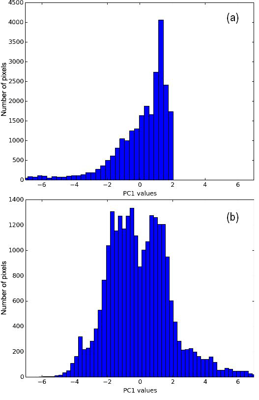
Figure 1 Probability distribution of PC1 before (a) and after the scaling and centring around the mean conversion (b).

Following the method of Z-score scaling (Johnson and Wichern, 1992) the values of principal components were scaled to 1 standard deviation centred on the mean. In addition, values of the first PC were converted so that the probability distribution of the values is closer to the Gaussian distribution (Fig. 1) using the following Eqs. (3) and (4).

$$\begin{array}{}\text{(3)}& {\displaystyle }& {\displaystyle }{P}_{\text{GAUSS}}={\log }_{\mathrm{10}}(min(P_{\mathrm{0}})-(P_{\mathrm{0}}\left)\right),\text{(4)}& {\displaystyle }& {\displaystyle }{P}_{\text{NORM}}={\displaystyle \frac{\left(\text{mean}\right(P_{\text{GAUSS}})-P_{\text{GAUSS}}){\mathit{\sigma }}_{\mathrm{0}}}{{\mathit{\sigma }}_{\text{GAUSS}}}},\end{array}$$

where P₀ denotes the original value of the first principal component, P_GAUSS denotes the value of PC1 after conversion to a Gaussian distribution, P_NORM denotes the values of PC1 after scaling and centring around the mean, σ₀ denotes the standard deviation of P₀ values and σ_GAUSS denotes the standard deviation of P_GAUSS values.

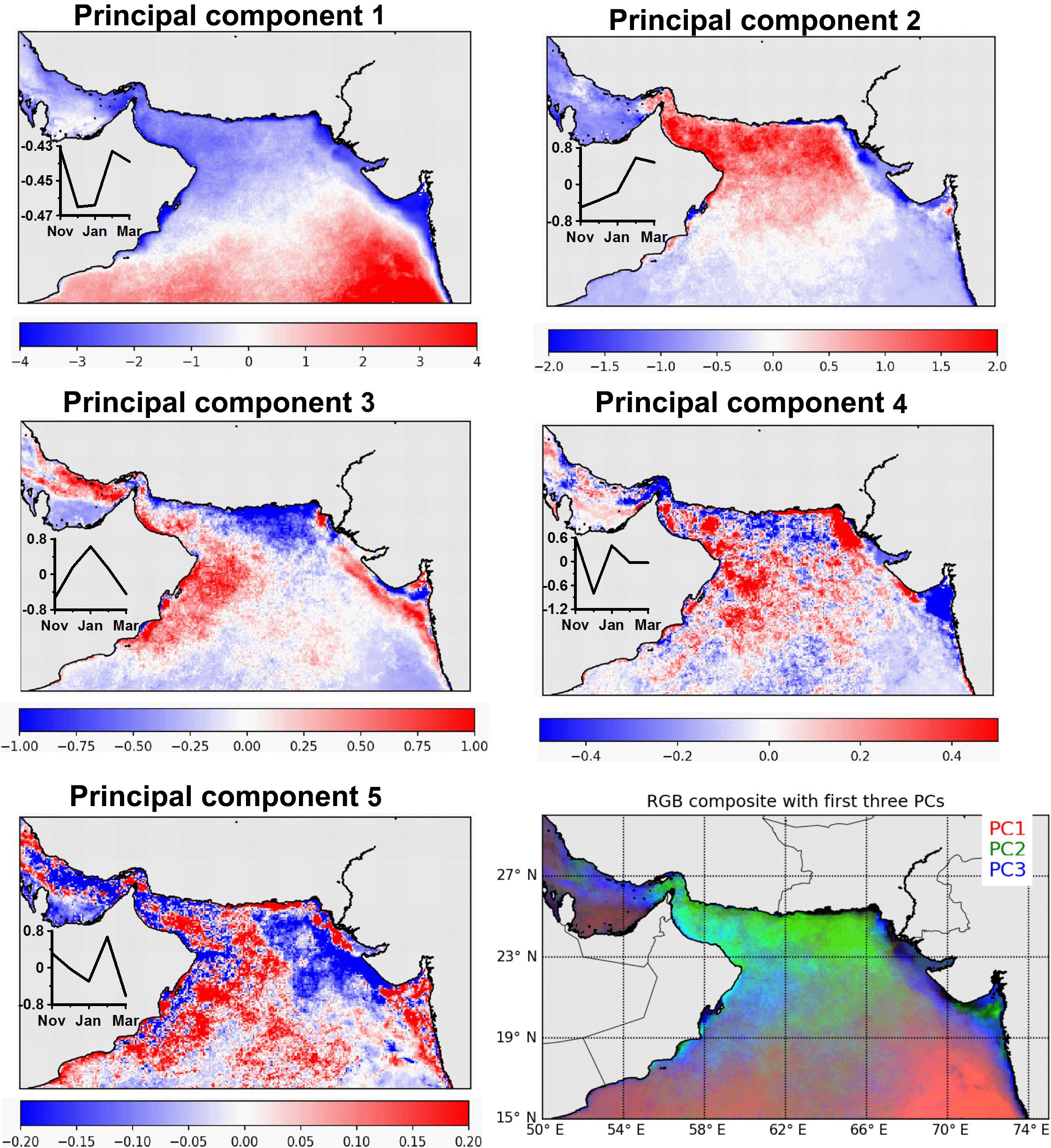
Figure 2 Individual maps of principal components (PC 1 to 5) and RGB composite of the first three statistically significant components. Corresponding to each PC, the respective periodicity is shown.

Maps of principal components (PC1-5) are examined with regard to spatial distribution, periodicity and information content (Fig. 2). Ranges of P_NORM decay from 8 (PC1), to 4 (PC2), to 2 (PC3), to 1 (PC4) and to 0.4 (PC5), confirming that most of the information about spatial and temporal dynamics of Chl a is retained in PC1. High values associated with PC1 are observed in the southern open-ocean part of the study area whereas low values are observed along coastal areas of western India and near the coast of Oman. This indicates the difference between ecosystem dynamics in the oligotrophic waters (southern open ocean) and those in the coastal eutrophic waters (coastal and northern area). The periodicity of PC1 indicates relatively constant negative values; thus PC1 is an expression of the overall pattern of low production in the southern oligrotrophic gyre and high production in the north and near the coast, which dominates the signal. Such a north-western to south-eastern gradient has been observed by Prakash and Ramesh (2007) in the study area using satellite Chl a. Jaswal et al. (2012) have reported a north–south gradient in the study area during winter, based on SST observations. PC2 indicates a semi-cyclic trend in Chl a production with its peak during February. The values develop from negative to positive with the same order of magnitude as PC1 and thus represents the main winter variability in the area. The strongest signal is in the north-western Arabian Sea extending up to the coast of Pakistan. The periodicity of PC3 also develops from negative to positive values and back to negative values in March. This PC demarcates the regions along the coast of Oman, west coast of India and northern part of the Persian Gulf from the other region where no significant peaks or minimums in Chl a occur during January. PC4 and PC5 represents the intraseasonal variability; the spatial signal is highly scattered for both these PCs and it is likely that they contain a considerable amount of noise. However, for PC4 we see consistent patterns along the coast of India and Pakistan and the signal is still about 10 and 5 % of the PC1 for PC4 and PC5 respectively. PC5 also differentiates Persian Gulf and the coasts of Pakistan and Gujarat from the rest of the north-central region. Based on this, PC1–PC5 was retained when considering possible zoning combinations (see Appendix A1); however, PC5 was not included in the final zoning.

To bring out the significance of combined PCs, a map (RGB composite of the first three statistically significant components) is drawn (Fig. 2f). This map is generated with the combination of the first three PCs (Fig. 2). The first PC is represented using red, the second by green and the third by blue. Zones with similar colours have similar combinations of PC values and therefore this figure illustrates similar winter variability of Chl a. This image is the application of a statistical clustering method to delineate the study region into areas with distinct Chl a dynamics based on the values of principal components as discussed in Sect. 3.

Figure 3 The identified ecological zones obtained from the combination of 4 PCs and 8 CAs.

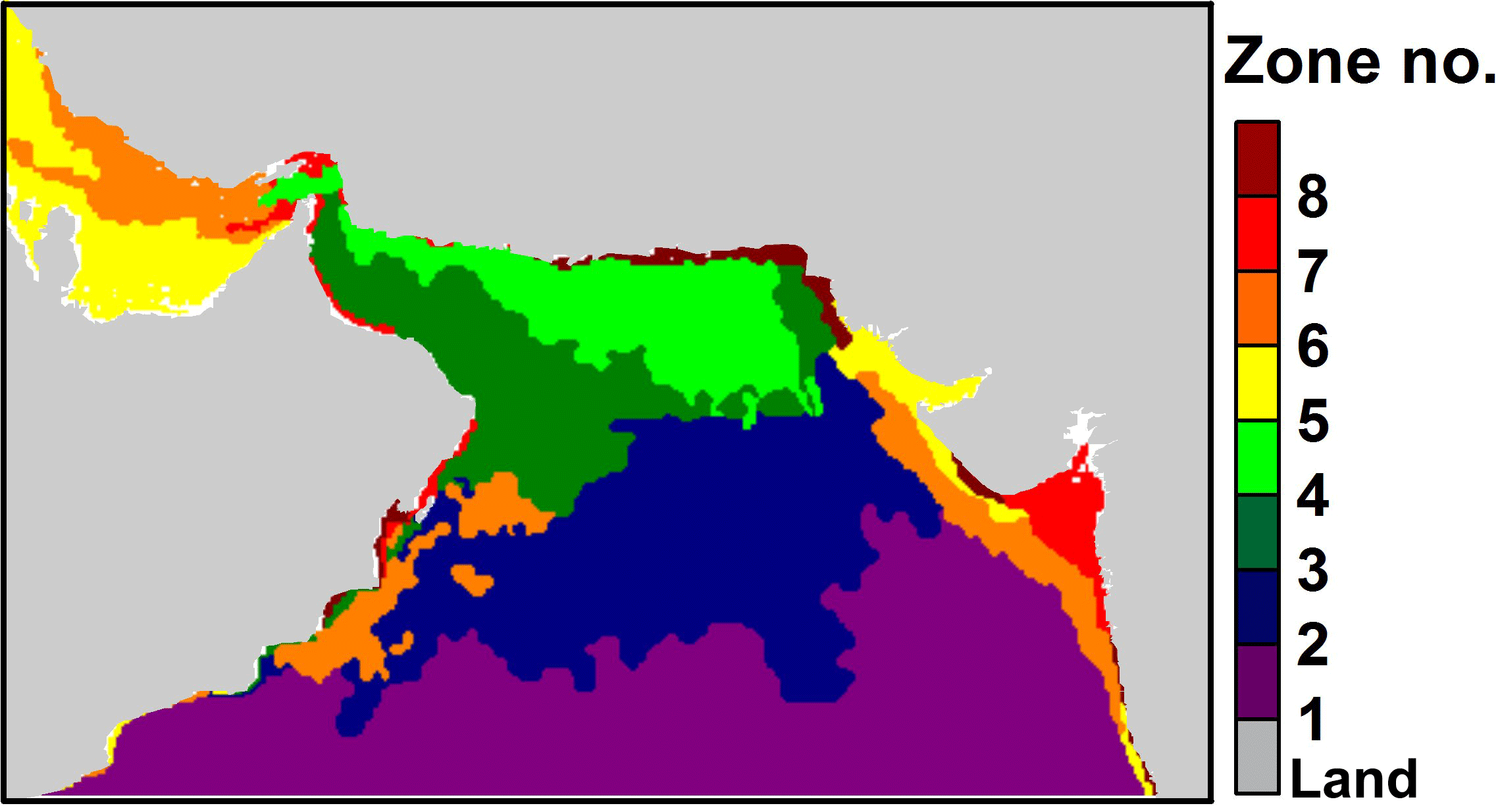
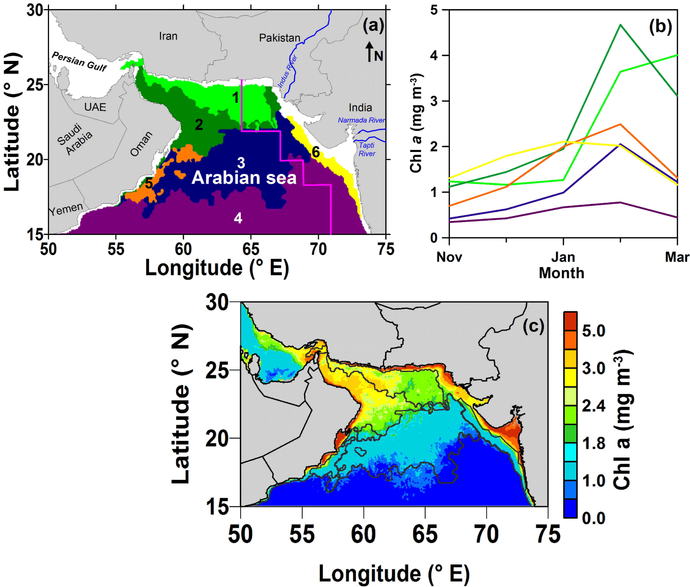
Figure 4 Map of the delineated ecological zones including the two Longhurst provinces in the northern Arabian Sea. Pink line demarcates the border between the Longhurst provinces in the study area, the north-west Arabian upwelling province to the west and the western India coastal province to the east, respectively. (b) The mean monthly climatology of surface Chl a concentration during the winter months, for each zone, plotted using the same colours as in (a) to represent each zone. (c) Annual winter climatology (seasonal average Chl a values over the winter period (November–March) from 2002 to 2013) of Chl a revealed from satellite data. The black lines indicate the boundaries of the delineated zones.

Several possible zoning maps were produced by varying the number of PCs and clusters in order to objectively delineate the northern Arabian Sea into ecological zones (Appendix A). The final delineation into ecological zones was obtained by combining the first 4 PCs and 8 clusters (Fig. 3), based on the general Chl a pattern in the northern Arabian Sea. Spatial smoothing was applied to the selected zone map. The methodology used in zone map selection and the smoothing procedure are provided in Appendix A. Satellite-derived Chl a values along coastal and shallow waters are found to be erroneous; hence, the coastal shallow water regions under zones 5, 7 and 8 as well as the part of zone 6 inside the Persian Gulf and patches along the coast of Yemen are excluded from further analysis in this study. This leaves the first four zones and the region in zone 6 along Oman and the west coast of India. Zone 6 has two regions that lie on opposite sides of the Arabian Sea, and the physical forcing affecting Chl a concentration along the two regions is likely to be different (Kumar and Prasad, 1996; Kumar et al., 2001; Shetye et al., 1994). Therefore, these two regions are considered as separate ecological zones. As a result, a total of six distinct ecological zones are delineated in the study area (Fig. 4a). It should be noted that due to the absence of relevant shipborne measurements and scarce satellite data, it is not possible to independently assess the accuracy of the delineation of the ecological zones.

4.1 Comparison of ecological zones with Longhurst provinces

Chl a winter variability revealed six distinct ecological zones in the Arabian Sea, which has been compared with the Longhurst biogeographical classification of marine provinces for the study area. The area analysed falls into two Longhurst provinces. These are respectively the north-west Arabian upwelling province (ARAB), covering the west and central part of the study area, and the western India coastal province (INDW) in the eastern part of the study area. The border between these two Longhurst provinces is demarcated with a pink line in Fig. 4a.

Zone 1 is located in the northern part of the study area (Fig. 4a). During winter, moderate (5–10 m s⁻¹) north-easterly winds blow over the area. Intense cooling is reported in this region, which enhances primary production (Kumar and Prasad, 1996; Madhupratap et al., 1996). Similar to zone 1, intense cooling and high production also occur in zone 2 (Madhupratap et al., 1996). The first three zones have a similar Chl a pattern, such that peak values occur during the month of either February or March, and for January Chl a concentration is always half of its peak value. These three zones are regions where strong convective mixing occurs during winter, which enhances Chl a concentration in these regions (Banse and English, 2000). The cool and dry north-easterly winds blowing onto the region from the adjacent land territories enhance cooling at the ocean surface. Consequently, increased evaporation leads to a decrease in surface temperature and an increase in surface salinity and density, creating convective mixing (Kumar and Prasad, 1996; Prasad and Ikeda, 2002; Shetye et al., 1992). All three of these ecological zones are stretched across both the Longhurst provinces, with the majority of the area located in the ARAB province. It should be mentioned here that the ARAB province with upwelling in the Arabian Sea according to Longhurst's classification represents provinces with strong upwelling during summer and with strong convective cooling during winter. The southern part of the study area includes zone 4, where winter cooling is less intense and less marine production occurs compared with zones 1–3 (Jyothibabu et al., 2010). However, similar to zones 1–3, zone 4 also is split across the two Longhurst provinces, with the western and central parts of zone 4 falling into the north-west Arabian upwelling province and the eastern part of the zone into the western Indian coastal province. Zone 5 includes the coastal area along the Oman coast between 18 and 22.5^∘ N, and the coastal region along the west coast of India from 16 to 23^∘ N is included under zone 6. These coastal areas are highly productive during winter (Kumar and Prasad, 1996; Kumar et al., 2001).

The physical mechanisms in the northern and north-western part of the Arabian Sea are very different from those in the eastern part. Strong convective mixing prevails in the northern and north-western parts of the study area. The strong stratification in the east, due to the presence of low-salinity and high-temperature water limits convective mixing in the eastern part of the study area (Naqvi et al., 2006). The eastern part comprises zone 6, a part of zone 3 and zone 4. Among these three zones, zone 6 is a coastal area and is vulnerable to coastal complex processes. Zone 6 is also an upwelling region (Shalin and Sanilkumar, 2014; Sudheesh et al., 2016).

For comparing Chl a in six zones using Longhurst's provinces, we have classified zone 1, zone 2, zone 3, zone 4 and zone 5 in the Longhurst ARAB province and zone 6 as the INDW province (Fig. 4a). Maximum Chl a observed during February is consistent in both provinces of Longhurst as well as the present six zones. During winter, ARAB (0.5–0.8 mg m⁻³) and INDW (0.4–0.6 mg m⁻³) have low values of Chl a with a similar range of variability (Longhurst, 2006). However, we have identified a high Chl a concentration (> 0.5 mg m⁻³) in the entire study area, with significant differences between various parts, particularly higher values to the waters closer to the coast. From our analysis, it is clear that the northern parts have higher concentrations of Chl a, with decreasing concentrations towards the south. Also, the variation between each zone was identified and showed higher concentrations of Chl a in the western zones compared to the more eastern zones. With only two Longhurst provinces, such a spatial difference is not detectable. This spatial difference is due to the difference in physical mechanisms as mentioned in the above paragraph. Longhurst classification is based on 1^∘ resolution global Chl a maps in the context of regional meteorological and physical oceanographic variability (Longhurst, 1995). It also uses Chl a observations from different time periods. In contrast, the present study utilises primarily Chl a concentration obtained from satellite sensors at about 100 times the resolution used by Longhurst for regional mapping and classification of ecological zones in the northern Arabian Sea. Hence, this regional classification could delineate the spatial Chl a variability better and the obtained zones contain more detailed regional information. This study is restricted to the analysis of data for the winter season. This work intends to characterise a more complete delineation of ecological zones and the mechanisms driving marine production in the study area during winter. Therefore, the influence of other ecological factors such as SST, MLD, PAR, wind and nutrients on Chl a production is included in the interpretations of the Chl a pattern in each of the ecological zones. The Longhurst classification accounts for the differences in physical conditions between the north-western and eastern parts. However, according to Naqvi et al. (2006), downwelling in the eastern part in winter cannot extend to the northern boundary of West Indian coastal province of Longhurst. Since the present zonal classification limits zone 6 from extending to the entire northern portion of the Longhurst province, our zones seem to be realistic in capturing regional Chl a variability during the winter season.

The annual winter climatology (seasonal average Chl a values over the winter period, November–March, from 2002 to 2013) of Chl a distribution revealed distinct features for each of the identified ecological zones (Fig. 4c). Based on the variability of Chl a concentrations, zone 1 experiences maximum bloom intensity between 1.5 and 9.6 mg m⁻³ with a mean of ∼ 2.6 mg m⁻³ and standard deviation of 0.7 mg m⁻³. Next to zone 1, high Chl a prevails in zone 2, with a range of 1.4 to 7.0 mg m⁻³ and a mean ∼ 2.8 mg m⁻³. Standard deviation observed in Chl a is the same for both zones. Moderate values of Chl a (1.3 to 1.9 mg m⁻³) are observed in zone 3, zone 5 and zone 6. Though similar ranges are observed for these three zones, the temporal evolution is different. In zone 3, Chl a varies between 0.5 and 4.2 mg m⁻³, with 0.3 mg m⁻³ standard deviation. Among coastal zones, zone 6 Chl a standard deviation is higher (0.8 mg m⁻³), with a range of 0.9 to 6.8 mg m⁻³, than in zone 5 (0.6 mg m⁻³), with a range between 1.0 and 4.3 mg m⁻³. Minimum value of Chl a for the winter is observed in zone 4 (0.2 to 1.2 mg m⁻³); in this zone the lowest mean (0.5 mg m⁻³) and lowest standard deviation (0.2 mg m⁻³) are also observed. The Chl a geo-spatial statistical variation in the study area clearly demarcates different ecological zones; however, in situ observations are scarce in the study region, and this limits the possibility to determine the accuracy of the satellite data and thus the accuracy of the delineated zones.

5 Time series analysis

Based on the magnitude of Chl a in each zone, time series data of Chl a and other environmental parameters (wind speed, MLD, PAR and SST) are examined to better understand the relations between physical and biological processes within each zone. Note that the influence of water temperature on primary productivity through control of metabolism and respiration is a highly non-linear process (Wetzel, 2001) and cannot be accounted for in the present study. Monthly climatology of Chl a concentrations in the identified ecological zones all have moderate to high values (0.3–5.0 mg m⁻³). Also, Chl a follows a semi-cyclic seasonal variation pattern during the winter months, with maximum values in February (Fig. 4b). In zone 6, peak Chl a is observed during January. Variability in the northern, most productive, part (zones 1 and 2) is discussed first and then the southern, least productive, zones (zones 3 and 4) are considered. Finally, the time series along coastal and continental shelf zones including zones 5 and 6 are examined. The mean and standard deviation for each of these parameters are calculated for each winter month (November to March).

5.1 The ecological zones in the northern and most productive part of the Arabian Sea

In general, Chl a concentration in zones 1 and 2 follows a typical wintertime cyclic variability with its peak values during the month of February (Fig. 5c). Throughout the study period, the Chl a concentration during February is at least double the concentration during January in these two zones. SST follows an inverse pattern compared with that of Chl a, such that SST minima coincide with Chl a maxima. Surface waters are relatively warm (> 27 ^∘C) during November and cool as winter progress, with stronger cooling in zone 1 and 2 (Fig. 5b). By January, SST has reduced by 2.5–3.0 ^∘C in both zones with a minimum of ≈ 23–24 ^∘C occurring in February. In March, the SST increases to 23–26 ^∘C. Although the Chl a range is approximately the same for both zones, comparatively SST is lower in zone 1 than zone 2. The inverse relationship between SST and Chl a have a weak correlation coefficient (correlation coefficients mentioned in this work are statistically significant at 95 % confidence interval) in zone 1 (r=0.39, n=60) and zone 2 (r=0.55, n=60).

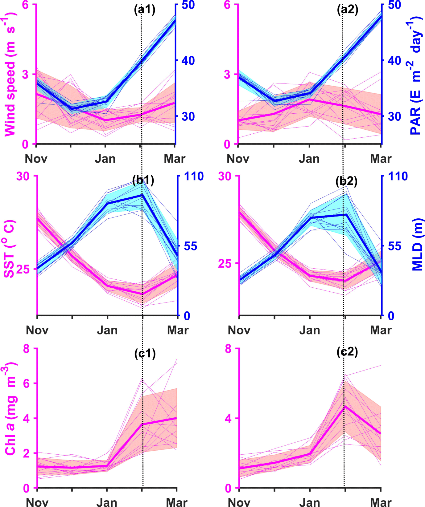
Figure 5 Temporal variability of wind speed and PAR (a), SST and MLD (b) and surface Chl a (c) averaged for zone 1 (left, denoted by suffix 1) and zone 2 (right, denoted by suffix 2) during the winter period for the years 2002–2013. Pink colour is used to represent Chl a, SST and wind speed and blue represents MLD and PAR. Thick lines represent means and the shaded areas the standard deviation for each parameter. The time series for the individual years are shown using thin lines. Vertical dotted lines represent the timing (month) of peak algae blooms in each zone.

A deepening of the MLD during winter is seen in both zones (Fig. 5b). During November, the MLD is shallow (≈ 35 m), and as winter progresses, MLD deepens to ≈ 80 m in January and in zone 1 to 90–110 m during February. In general, the MLD in zone 2 is about 10 m shallower than in zone 1 during January and February. The MLD starts to become shallow again in March. The peak concentrations of Chl a coincide with the deepest MLD. However, MLD and Chl a in zone 1 and 2 are moderately correlated (correlation coefficient, r=0.28).

During winter in the study area, SST cooling initiates MLD deepening. The decrease in SST is mainly due to evaporation, which has dual effects, i.e. increase in salinity and reduction in temperature, causing increased density of surface water (Naqvi et al., 2006), as a consequence of which convective overturning takes place. As winter progresses, SST drops and convective overturning occurs (salinity and temperature effect), increasing the MLD (Shankar et al., 2015). MLD also influences SST variability. For example, when the MLD deepens, SST will decrease as cool water is mixed toward the surface. On the contrary, during a shallow MLD, SST is generally higher (Cronin and Kessler, 2002). Hence, both of these environmental parameters are dependent on each other and both influence marine primary production in the study area. Wind speed fluctuates strongly for zones 1 and 2. In zone 1, the maximum variability (0.5–3.0 m s⁻¹) is seen during November and December and for zone 2, the wind varies strongly throughout winter, with maximum wind speed (0.5–3.0 m s⁻¹) for December and January (Fig. 5a). High inter-annual variability is seen in wind speeds along the two zones, with peak wind speed in any one of the months between November and February. Only in certain years did moderate wind (< 3 m s⁻¹) coincide with high Chl a, and the correlation coefficient confirms that Chl a and wind speed are not correlated in zone 1 and 2 (r=0.09, n=60).

PAR follows the seasonal cycle of incoming solar radiation (Arnone et al., 1998). PAR is the waveband of light that is used in photosynthesis, and it is closely correlated with total incoming solar radiation heating the water column. Hence, an increase in PAR is accompanied by higher surface temperatures and associated with enhanced stratification, which results in reduced mixing and vice versa (Lee et al., 2014). Decreasing PAR (33–36 E m⁻² day⁻¹) prevailed in the study area during November to December for both zones, which corresponds to a decreasing trend in temperature and a deepening MLD cycle. Contrarily, when PAR increased after December, surface temperature started increasing and mixing was reduced. However, there is a 1-month time lag between the onset of increasing PAR and the onset of increasing SST. The increase also coincides with a reduction of the MLD. This is due to the high heat capacity of water and the large amount of energy required to heat the water column when the MLD is deep. Low SST and deep MLD favours increased nutrient supply to the euphotic zone (Madhupratap et al., 1996; Wiggert et al., 2000) and hence production increases in these zones by February. These transitions, in terms of a reduction in SST and peak MLD, initialise algal blooms. Hence, PAR also influences production indirectly, by affecting the stratification that controls nutrient availability. There is stronger correlation between Chl a concentration and PAR in zone 1 (r=0.69, n=60) compared to zone 2 (r=0.49, n=60).

Peak Chl a concentrations occurring during February coincided with the lowest SST (< 25 ^∘C) and deepest MLD (90–110 m). Thus, the increased amount of Chl a is found to be directly related to sea-surface temperature variability (i.e. cooling) and the deepening of the mixed layer. A similar inverse relation between productivity and SST is observed in the Indian Ocean by Singh and Ramesh (2015). PAR was found to have an indirect influence on primary production in these zones. PAR increases surface temperature and as a result mixing gets reduced and vice versa. During the month of January, PAR increase coincides with SST reduction and MLD deepening, with the increase in PAR starting about 1 month before the reduction in SST and deepening of MLD. SST reduction and MLD deepening increases nutrient supply to the mixed layer, thus enhancing production. Nitrate is high at 100 m depth (> 12 µmol L⁻¹), and thus a deepening of the mixed layer beyond 100 m will mix up nutrients towards the surface (Garcia et al., 2013). This suggests that the highest Chl a concentrations are due to the increase in nutrients by a deepening of the MLD triggered by cooling (Figs. 5, 6, 7, 9) in December and January. Wind influence is not strong in these zones. Though the wind speed is relatively low (< 2 m s⁻¹) during most years, certain cases with moderate wind speed (≈ 3 m s⁻¹) are observed in these zones. Moderate wind (5 m s⁻¹) occurring during January to February could have enhanced mixing and thus production in zone 2.

5.2 The ecological zones in the southern and western Arabian Sea

Chl a, SST, MLD and PAR values in zones 3 and 4 followed similar seasonal patterns of variability to those in zones 1 and 2 (Fig. 6). However, the range of values are different in these zones compared with the ecological zones further north. The magnitude of Chl a concentration in zone 3 is 2 to 3 times less than in zones 1 and 2 and Chl a in zone 4 is about half of the Chl a concentration in zone 3. Thus, the Chl a concentrations occurring in zones 3 and 4 differ from the first two zones. The inter-annual variability of SST, MLD and PAR is higher in the third and fourth zones compared to the two zones further north. In zone 3, as it is closer to the Equator, PAR is 3–4 E m⁻² day⁻¹ higher, SST is 1.5 ^∘C warmer and MLD ≈ 10–15 m shallower than in zones 1 and 2. Furthermore, PAR in zone 4 is 2–3 E m⁻² day⁻¹ higher, SST is 1.0 ^∘C higher and MLD is 10 m shallower than in zone 3. The fact that Chl a concentration in zone 3 is less than in zones 1 and 2, and Chl a in zone 4 is still lower than that in zone 3, affirms that variation in Chl a production in the northern Arabian Sea is strongly related to physical parameters viz. SST, MLD and PAR. SST is an indirect indicator of favourable conditions for algal blooms. Low SSTs can be the result of intensified convection, which will also be manifested by increased mixed-layer depth and entrainment of waters rich in nutrients (Morrison et al., 1998). The warmer SSTs in zone 3 and 4 indicate that the rate of convection is most likely weak in zone 3 and even weaker in zone 4 compared to zones 1 and 2. This indicates that phytoplankton production in these zones could be linked to the convectional strength and increase in nutrients and that the production is limited by nutrients in the period before and after the bloom. In zone 3 and zone 4 the inverse correlation between SST and Chl a is stronger compared to zone 1 and 2, with r=0.62 and 0.70, respectively.

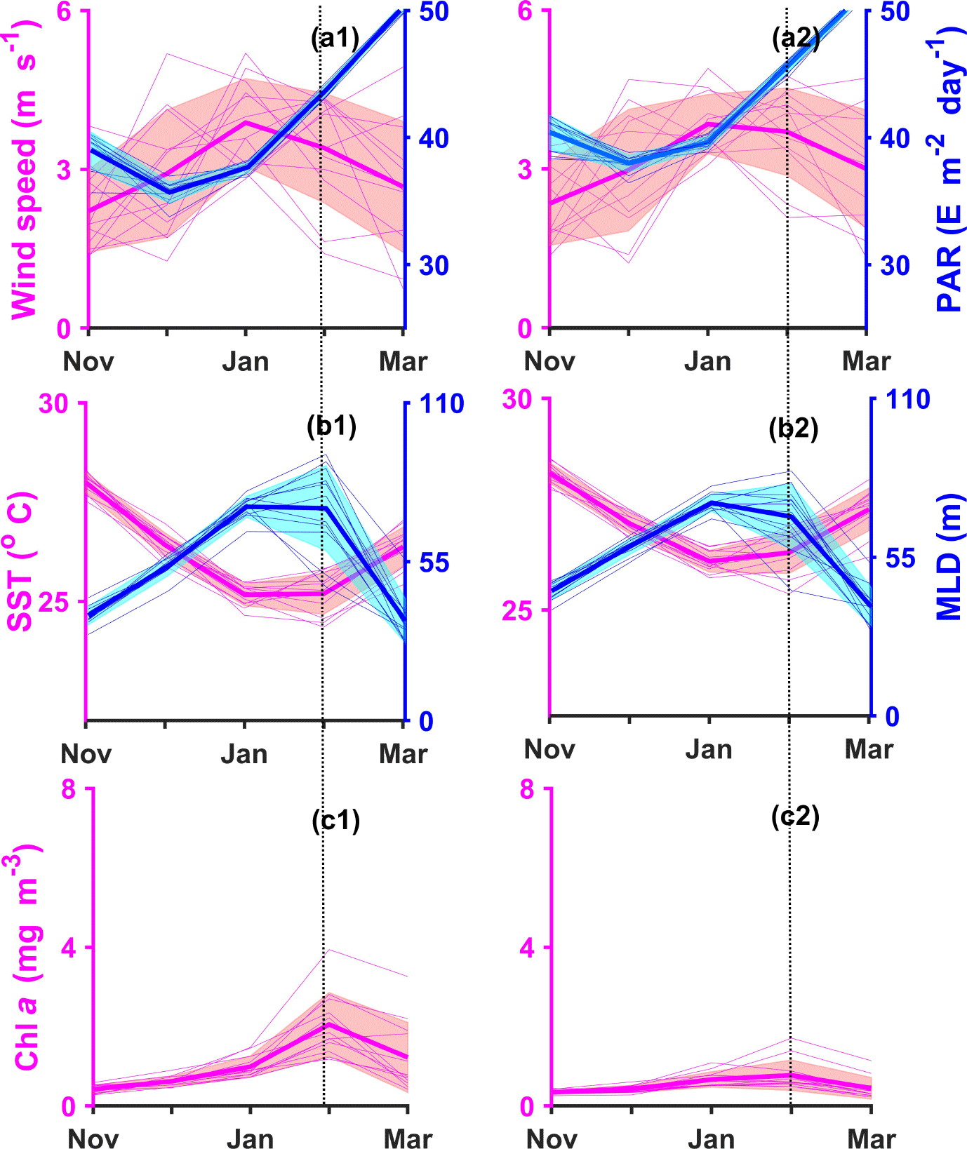
Figure 6 Temporal variability of wind speed and PAR (a), SST and MLD (b) and surface Chl a (c) averaged for zone 3 (left, denoted by suffix 1) and zone 4 (right, denoted by suffix 2) during the winter period for the years 2002–2013. Pink colour is used to represent Chl a, SST and wind speed and blue represents MLD and PAR. Thick lines represent means and the shaded areas the standard deviation for each parameter. The time series for the individual years are shown using thin lines. Vertical dotted lines represent the timing (month) of peak algae blooms in each zone.

The availability of nutrients is the prime factor influencing production. A deepening of the mixed layer will increase nutrient availability, but the magnitude depends both on the depth of the MLD and on concentration of nutrients below the mixed layer. The relatively shallow MLD and high SST in zones 3 and 4 compared with zones 1 and 2, suggests low transport of nutrients into the mixed layer in zones 3 and 4 compared to the other two zones. MLD and Chl a productivity in zones 3 and 4 are correlated (r=0.50, n=60 and r=0.56, n=60, respectively). The indirect influence of solar radiation in maintaining SST and MLD and thus nutrient availability is evident from higher PAR, higher SST and more shallow MLD values in zones 3 and 4 compared with zones 1 and 2. Hence, a direct dependence of SST cooling and deepening of the MLD and indirect dependence of PAR on the primary production is evident in the first four zones. In zone 3, a weak correlation exists between PAR and Chl a (r=0.41, n=60), and in zone 4 these two parameters are not correlated at all. The increasing wind speed pattern prevalent during winter indicates that wind mixing could be the prime factor governing the ecological dynamics in this zone during winter. Chl a has a weak positive correlation with the wind speed in zone 3 (r=0.30, n=60) and moderately correlated in zone 4 (r=0.47, n=60). A relatively warm surface and shallow mixed layer in zone 4 indicate weak convective overturning (Naqvi et al., 2006). Hence, wind-induced mixing in this zone can influence production.

5.3 The ecological zones in the coastal and continental shelf waters

Elevated values of Chl a (> 2.5 mg m⁻³) persist in zones 5 and 6 throughout the winter season, with high levels of variability. This suggests that the dynamics in the coastal and continental shelf zones 5 and 6 are more complex than open-ocean waters (zones 1, 2, 3 and 4). Chl a in zone 5 shows significant inter-annual variability for the winter period with its peak value during February. In zone 6 there is low variability of Chl a for the winter period in January, while the range of variability is high for both December and February. In zones 5 and 6, MLD maxima and SST minima occurred either during January or February (Fig. 7b). During January and February, in zone 5 MLD varied between 70 and 80 m, and in zone 6, MLD varied between 80 and 100 m. A comparison between MLD values in zones 5 and 6 with those in zones 1 and 2 shows that MLD is shallower in zone 5, whereas the variability of MLD in zone 6 is comparable to that in the first two zones. MLD variability for the winter is consistent with Longhurst's observations; however, the range of MLD in Longhurst is smaller (range from 40 to 70 m) compared to present study (40–110 m) for the winter period. Additionally, SST is higher during January–February in zones 5 and 6 (> 24.5 ^∘C) compared to SST values in zones 1 and 2 (23.5–24.5 ^∘C). The correlation coefficient between MLD and Chl a is lower in zone 5 (r=0.53, n=60) than in zone 6 (r=0.69, n=60). However, the inverse relation between SST and Chl a concentration is higher in zone 5 ($r=-\mathrm{0.64}$, n=60) compared to zone 6 ($r=-\mathrm{0.54}$, n=60). PAR ranges for December and January in zones 5 and 6 are almost equal to PAR ranges in zones 3 and 4 (36–38 E m⁻² day⁻¹) and are higher compared to zones 1 and 2 (30–34 E m⁻² day⁻¹) for the same period. A weak inverse correlation ($r=-\mathrm{0.27}$, n=60) exists between PAR and Chl a in zone 6, while in zone 5 these parameters are not correlated (r=0.12, n=60). For zone 5, wind and Chl a production are weakly correlated (r=0.30, n=60), while in zone 6, these parameters are not correlated ($r=-\mathrm{0.09}$, n=60).

In zone 5, low SST prevails, which is an indicator of strong convective activity. Again, in zone 6, high SST coincides with deep MLD and strong wind. Wind is reported as the one of the main forcing factors in the INWM by Longhurst (2006), which is consistent with our present study. Comparatively warm surface water indicates convective overturning is weak, and in addition the presence of strong wind suggests production in this zone could be controlled by upwelling induced by wind. Production in zone 6 was found to be more complex with the influence of wind. Gandhi et al. (2011) and Kumar et al. (2017) indicate that nitrogen fixation may provide a significant contribution to production in zone 6. However, the results are based on experiments with limited temporal coverage.

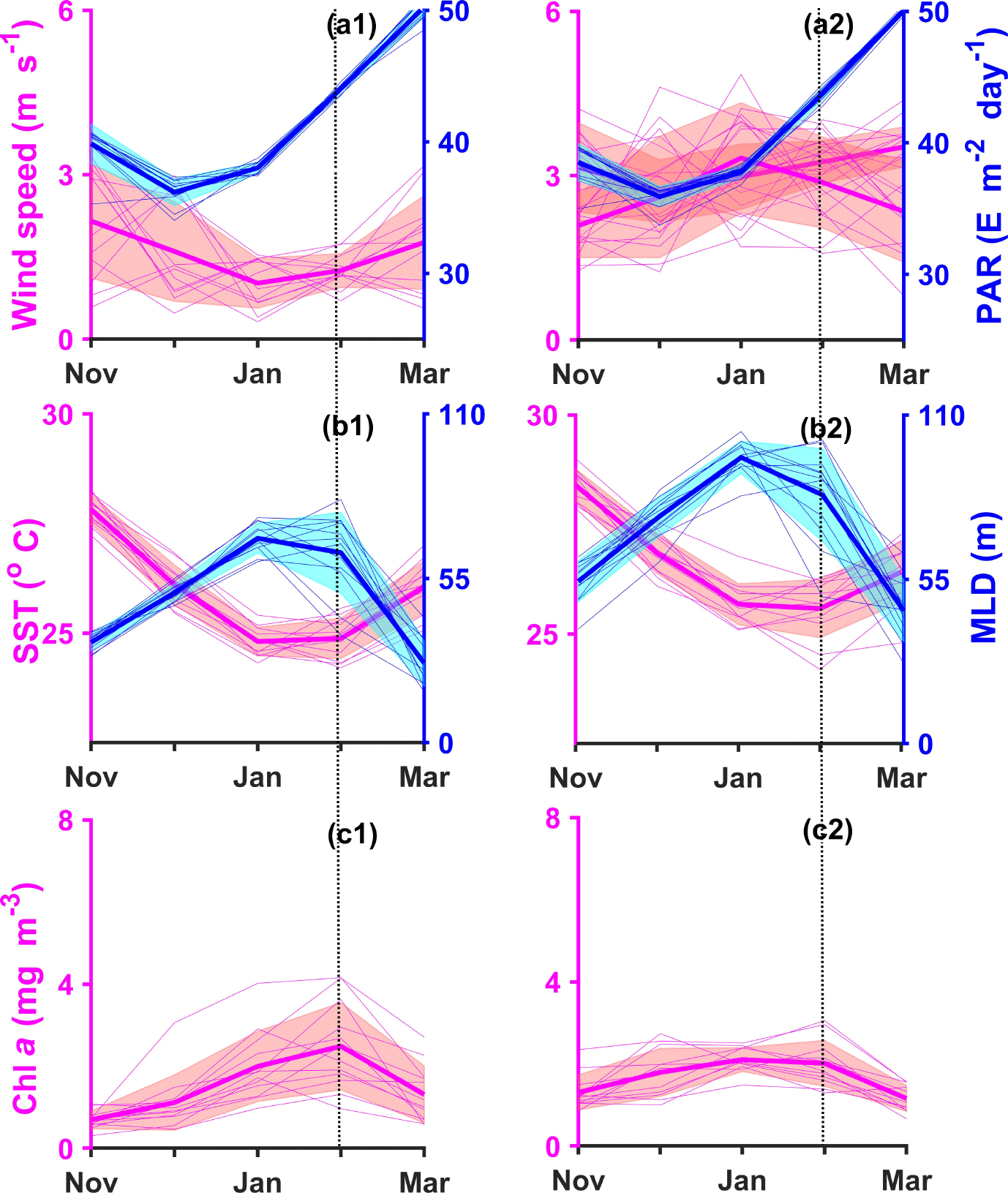
Figure 7 Temporal variability of alongshore wind speed and PAR (a), SST and MLD (b) and surface Chl a (c) averaged for zone 5 (left, denoted by suffix 1) and zone 6 (right, denoted by suffix 2) during the winter period for the years 2002–2013. Pink colour is used to represent Chl a, SST and wind speed and blue represents MLD and PAR. Thick lines represent means and the shaded areas the standard deviation for each parameter. The time series for the individual years are shown using thin lines. Vertical dotted lines represent the timing (month) of peak algae blooms in each zone.

5.4 Multiple linear regression analysis

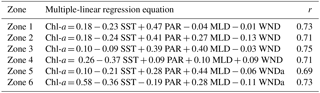
Multiple linear regression analysis is carried out to understand the combined effect of all chosen environmental parameters on Chl a production. Multiple linear regression (MLR) is performed here on normalised values of selected parameters, such that individual values are subtracted from the minimum value of observation and then divided by the range of observation. MLR equations with r values are tabulated in Table 1. The MLR equations for all six zones are found to be statistically significant and are carried out using 60 data points. WND represents wind speed and WNDa the wind speed alongshore component in the coastal zones (zones 5 and 6).

In general, MLR analysis confirms that production is controlled by surface cooling, enhancement of PAR and deepening of MLD. However, the dependence of each of these variables differs within each zone. A negative impact of wind is observed in the first three zones and a positive influence of wind in the last three zones. As for zone 5 and 6, alongshore wind components are considered, and the southward component enhances production in these cases. However, the negative wind speed coefficient observed for first three cases may be due to the fact that the time span considered in this work is monthly and the effect of wind occurs on shorter timescales. In the first zone, for a 1 % (0.01) increase in normalised light availability as well as a 1 % normalised cooling increased the Chl a concentration by 0.0047 and 0.0023 mg m⁻³ respectively. In the second zone PAR had the most influence on production (for each 1 % increase in PAR chlorophyll increased by 0.0041 mg m⁻³), followed by MLD and SST. For the third zone, MLD and PAR have the highest influence on Chl a. Cooling has a major influence in the fourth zone. In the fifth zone, MLD, PAR and SST have major control of production, similar to zone 2; however, the rate of enhancement differs between these zones. In zone 6, cooling also has a major influence, which is followed by a PAR decrease and MLD deepening. An inverse relation of PAR to Chl a is observed in this zone. It should be mentioned here that, unlike in the other five zones, two Chl a maxima, SST minima and a deepening of MLD with an initial peak are observed during December. PAR has its minima during this initial bloom month and an increasing trend corresponding to the second peak of Chl a, i.e. the bloom occurs during its minimum and maximum values of PAR winter cycles. This implies PAR is not a limiting factor for production in this zone.

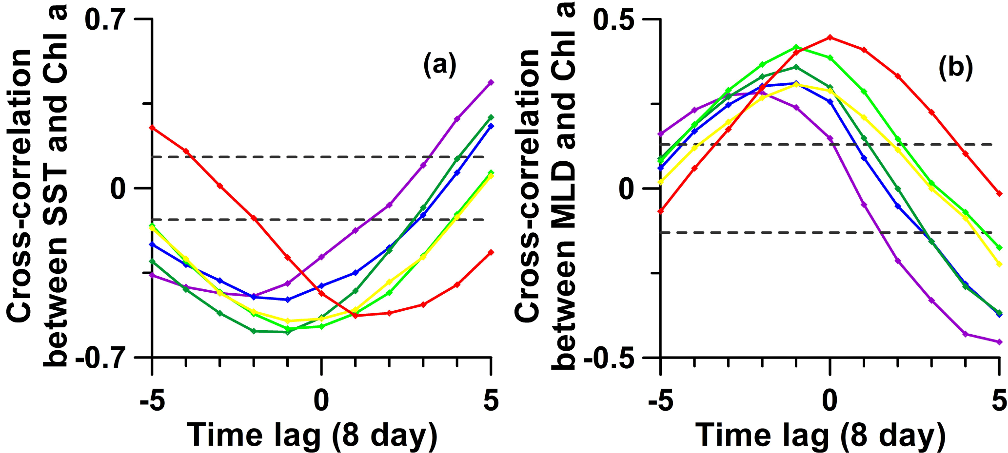
Figure 8 Cross-correlation of (a) SST and (b) MLD with Chl a in six zones. Grey dashed horizontal line represents the 99 % confidence interval. Each unit on the x axis represents an 8-day period. Zones 1–6 are represented by violet, blue, green, light green, yellow and red lines respectively.

Table 1 Multiple-linear regression analysis.

6 Time lag between SST and MLD variability to peak algae bloom

It is evident from the above analysis that Chl a production depends strongly on cooling intensity (variability of SST) and MLD development. To quantify the eventual lag between SST minimum and MLD maximum to Chl a maximum, the time-lagged correlations of each of these parameters with Chl a are calculated (Fig. 8). As these parameters influence algal blooms on a shorter timescale than a month, these analyses are carried out using 8-day composite data. Cross-correlation analysis shows (Fig. 8 and Table 2) that zones 1 to 5 reveal a strong and significant (p<0.01) correlation between Chl a values, and SST occurs with lag of −3 to −1 time interval (a scale = 8 days), i.e. a dip in SST occurs before the peak in Chl a. A similar situation is observed for MLD but the lag is shortened by one time step, i.e. 8 days. In zone 6, an SST maximum is observed 1 time step later than the Chl a maximum (lag = 8 days) and MLD peaks simultaneously with Chl a (lag = 0). These observations enable us to put forth a hypothesis that the prevailing cool conditions must have enhanced mixing in the study area, which led to increased algae production.

7 Impact of nutrients and iron on Chl a production based on the analysis of climatological nutrient and dust optical thickness

The time lag between Chl a maxima and MLD maxima suggests that enhanced nutrient availability in the water column due to a deepening of the mixed layer could lead to increased primary productivity. However, the time lags between MLD and Chl a varied for the six zones, implying productivity is not only dependent on nutrient availability, but also on other environmental variables (Table 2). Naqvi et al. (2010) reported that iron limits the marine productivity along the Oman coast, which corresponds to the north-western part of the study area. Similarly, Banerjee and Kumar (2014) have also reported marine production limited by availability of iron in central Arabian Sea. Hence iron supply to the ocean surface have been analysed using the DOT, where high DOT indicates more iron deposition from the atmosphere. The temporal variability of nitrate in the mixed layer and DOT from the atmosphere is compared with the Chl a variability in each ecological zone (Fig. 9). Nitrate and DOT show significantly different patterns of seasonal variability in each zone. Wiggert et al. (2006) parameterised nitrogen half-saturation constants in the northern Indian Ocean to 0.4 µmol L⁻¹ for small phytoplankton and 0.8 µmol L⁻¹ for large phytoplankton. The climatological data show that nitrate < 0.8 µmol L⁻¹ was observed only in March (zone 1) and November (zone 6), which shows that usually nitrate is not a limiting factor.

Table 2 Lag between peak Chl-a, SST and MLD in 8-day intervals.

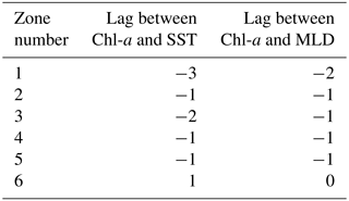
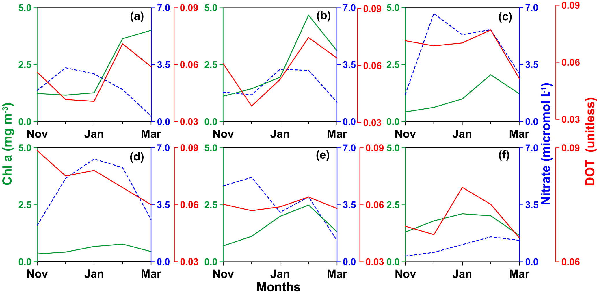
Figure 9 Averaged variability of surface Chl a, nitrate and DOT in six ecological zones. Panels (a)–(f) represent variability along the first to sixth zones, respectively.

High amounts of nitrate can contribute to the production of large algal blooms (Pondaven et al., 2000; Wiggert et al., 2006). These can also be harmful and are abundant in the eastern Arabian Sea (Singh et al., 2014). However, our observations indicate that higher nitrate does not always correspond to elevated Chl a concentrations. For example, during the months of December and January high nitrate availability (> 2 µmol L⁻¹) prevails for zones 1–5, while biological activity is moderate (Chl a < 3.0 mg m⁻³), suggesting that additional variables play a role in determining primary production. The fact that, during each of the algal blooms (Chl a > 1.5 mg m⁻³), both nitrate (> 3 µmol L⁻¹) and DOT (> 0.11) had high values confirms that the co-occurrence of high concentrations of these two nutrients is necessary to enhance primary production. Interestingly, Chl a and DOT followed a similar pattern of variability from January to March for zones 1–3 and 5. The fact that Chl a follows a similar temporal pattern as DOT in zones 1, 2, 3 and 5 strongly indicates that iron is a limiting factor for productivity in these zones. This result is in agreement with Wiggert et al. (2006) and Naqvi et al. (2010), who show that iron limits production in the northern and north-western parts of the Arabian Sea. In zones 4 and 6, which lie to the south and south-east, the relationship between iron and Chl a is not evident. Aerosol in the south and east has much lower iron content compared to the western part (Appendix A3). To quantitatively analyse the impact of atmospherically deposited iron in the study area, comprehensive in situ measurements of the iron content at the sea surface are required, and these are presently not available.

8 Summary and conclusions

In this study a statistical objective zoning methodology was applied to remotely sensed Chl a data for the northern Arabian Sea, and eight homogeneous ecological zones were delineated. In six of these zones Chl a variability is studied in relation to physical–chemical parameters. Despite limitations in the accuracy of the delineated zones, the identified six ecological zones give an improved picture of the variability of marine ecosystems during winter in the Arabian Sea compared to the Longhurst classification in two provinces for the entire northern Arabian Sea (Longhurst, 2006). The Chl a variability followed a semi-cyclic pattern during the winter period, with the mean of peak observations for the study period observed during February in zones 1 to 5 (Fig. 4). For zone 6, there is no distinct peak value between December and February. Zones 1 and 2 in the northern part of the Arabian Sea were highly productive (Chl a values ranging from 1 to 7 mg m⁻³), while zone 3 (1–4 mg m⁻³) and zone 4 (1–2 mg m⁻³) were found to be less productive, i.e. a north–south gradient in the phytoplankton productivity is observed. Contrary to the open-ocean zones, the coastal and continental shelf water zones, zone 5 and zone 6, have high levels of variability, with elevated Chl a values throughout winter (> 2.5 mg m⁻³). In addition, the inter-annual variability for the winter season is well captured in the present study and is not seen in Longhurst's case. This is because in the present analysis delineation is done considering winter period alone, while in case of Longhurst the annual variation is considered for delineation. Moreover, this study is assessed for 11 years, while Longhurst's is for about 4.5 years (Longhurst, 2006).

Chl a production in the delineated zones within the study area is controlled by surface cooling, an increase in PAR and deepening of MLD. MLR analysis confirms the varying dependence for each of these three variables within each ecological zone. However, the influence of wind speed is not visible from monthly data; to understand wind dependence on Chl a, a much shorter timescale is required, as wind dependence occurs on scales less than a month. The combined analysis of DOT and nitrate suggests that the variability of the algae concentration depends on both sources of nutrient supply in all six identified ecological zones. However, the variability of Chl a in the northern and north-western parts of the Arabian Sea (zones 1, 2, 3 and 5) is predominantly correlated with the atmospheric deposition of iron during the period from January to March.

The satellite-based Chl a concentration utilised in this work is a proxy of marine primary production, and the results obtained in this work are consistent with those of Singh and Ramesh (2015). Their paper states that nutrients and solar radiation are predictors that can explain most of the variability in the marine productivity, and they observed a strong inverse relation of primary production with SST.

In the absence of comprehensive and spatio-temporally complete in situ and satellite remote sensing data sets, this study provides a more comprehensive understanding of the environmental factors controlling the spatio-temporal variability of the marine Chlorophyll a concentration in the northern Arabian Sea during winter conditions. Considering the availability of long time series of high-resolution satellite Ocean Color data and biogeochemical numerical ocean models today, this study is timely. Additionally, this study reveals the need for better understanding of factors controlling the marine primary productivity in other coastal upwelling zones. The north Arabian Sea is not well sampled and more in situ observations are needed in order to validate remote sensing products and initialise numerical models and establish more reliable databases. Biogeographical studies of the lower trophic level of the marine ecosystem, such as this one, could be used to design new sampling programs and strategies.

Appendix A

A1 Various combinations of PC and cluster numbers for performing zoning

As the first three PCs account for 97 % of the total Chl a variability in the study area, it is compulsory to consider at least the first three PCs for zoning. Hence, in the present study various possible combinations of PCs viz. the first three PCs, first four PCs and first five PCs are selected to map Chl a zones. Varying complex coastal dynamics (including high Chl a along the coast of the Arabian Peninsula, river discharge from Indus river along Pakistan and western Indian coast and high sediment distribution and river discharge from the Narmada and Tapi rivers along the coast of Gujarat) suggest at least three ecosystem zones along the coastal regions (Chandramohan and Nayak, 1991; Singh and Ramesh, 2011). High-saline waters in the Persian Gulf have different dynamics compared to the rest of the study area, suggesting at least one zone in the Persian Gulf. Furthermore, in the open ocean at least two zones are proposed: one in the north and another in the southern sectors (Gomes et al., 2008). Thus, based on the dynamics in the area, at least six distinct zones are identified in the study area. Initial preliminary images showed cluster number nine and above have insufficient clustering and therefore, cluster number (c) chosen here, is six to eight (Fig. A1).

Various combinations of PCs and clusters are carried out using 3 to 5 PCs and 6 to 8 clusters. The number of PCs selected is hereafter suffixed using the letter “p” and the number of clusters by “c”. The selected nine combinations of PCs and cluster numbers include (1) 3pc 6c, (2) 4pc 6c, (3) 5pc 6c, (4) 3pc 7c, (5) 4pc 7c, (6) 5pc 7c, (7) 3pc 8c, (8) 4pc 8c and (9) 5pc 8c (Fig. A1). In general, zone maps obtained from the nine selected combinations classified the Persian Gulf into two zones, the offshore area into four zones and the areas within bathymetry depth 150 m as coastal zones. Open-ocean areas are demarcated using blue and green parts of the spectrum, while coastal areas are demarcated by yellow, orange and red colours. In seven out of the nine zone maps (1: 3pc 6c; 2: 3pc 7c; 3: 4pc 6c; 4: 4pc 7c; 5: 5pc 6c; 6: 5pc 7c; and 7: 5pc 8c) the lower portion of Persian waters and southern part of the area are represented as a single zone. However, it is known that the dynamics of these two regions are entirely different (Bower, 2000; Shankar et al., 2002) and hence these zone maps are not selected for the present study. The zone map with the 3pc 8c combination (red patch), which in general represents the coastal region, is not restricted within 150 m depth. Hence, this zone map is also discarded, leaving the zone map with combination 4pc 8c to be selected for the present study.

A2 Spatial smoothing on the selected zone map

In the selected zone map, overlapping zones are observed, especially in the central study area. Zone 1, zone 2, zone 3 and zone 4 as well as the orange patch along the Oman coast are highly scattered and hence each of these are overlapped one over the other. Simple averaging will remove the characteristic features along highly overlapping regions and hence will cause smoothing, i.e. the border of each of these highly scattered zones are identified before averaging. Smoothing considers an area with a 5 × 5 pixel. Each middle pixel is replaced by the zones with major pixel characteristics. Along the coastal area, pixels with more than five consecutively similar values are considered, while others are replaced with the main zonation along the area. After smoothing, averaging is applied around a 3 × 3 pixel area, such that characteristics of pixels with half or more strength are considered; otherwise they are replaced by the main zone.

A3 Winter wind roses

In order to better understand why DOT is higher in some parts of the sea than in the others, wind roses are plotted alongside with DOT over the study area (Fig. A2). The Arabian desert in the west and Thar desert to the east are the major dust-contributing deserts to the study area. As suggested we have plotted the wind roses for the respective zones in order to reveal the possible source locations of DOT. For zone 1, both the Thar desert and Arabian desert contribute to DOT, as the strong winds have directions between northerly and north-westerly. Similarly for zone 2, both these zones can be significant. For zone 3, the Arabian desert contributes more to DOT enhancement, as revealed from wind rose diagram, while for zone 4, the contribution is brought by continental winds from the Indian sub-continent. This is consistent with Patel et al. (2017).

Figure A1 Various combinations of PC and CA tried out for achieving better zonation.

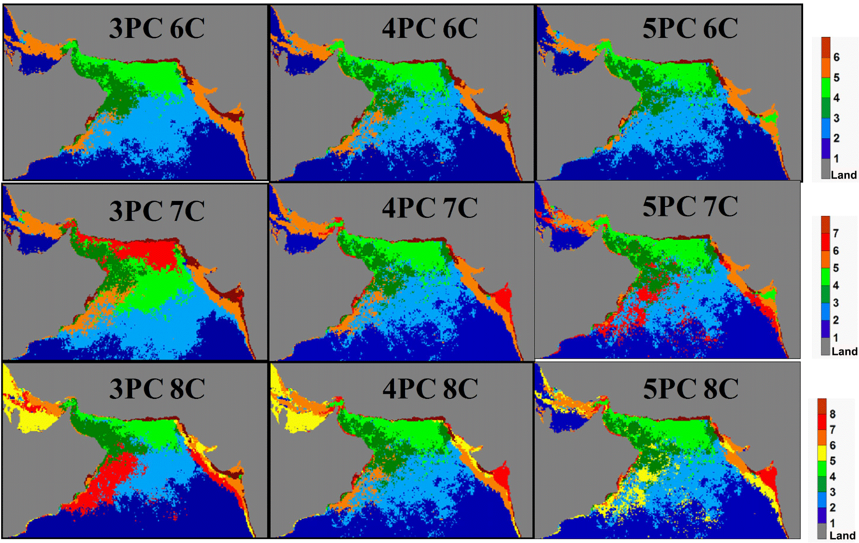
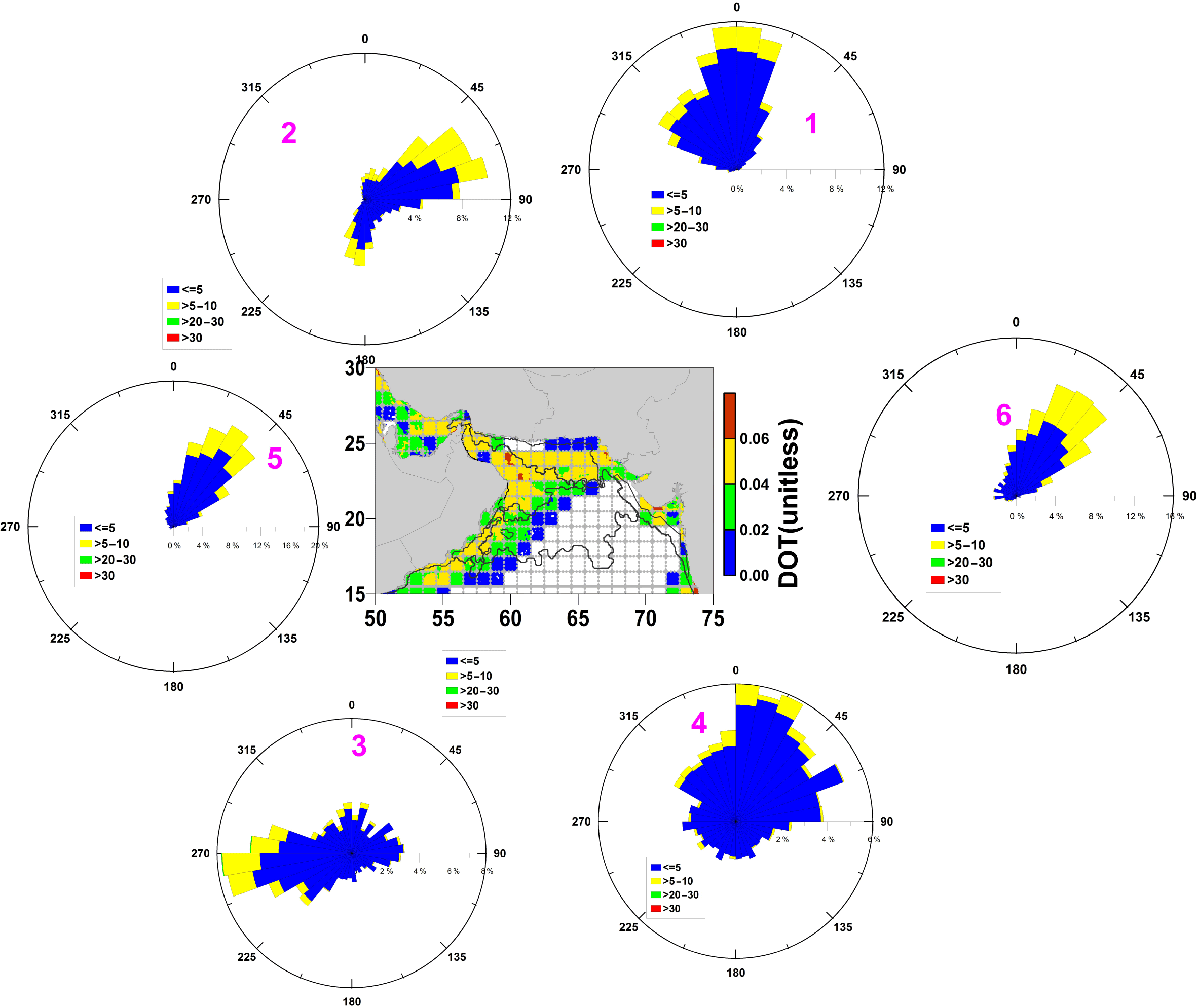
Figure A2 Wind rose diagram for the six zones. Zone number corresponding to wind rose plot is provided in pink colour.