the Creative Commons Attribution 4.0 License.
the Creative Commons Attribution 4.0 License.
 | 26 Mar 2018
Species composition and forest structure explain the temperature sensitivity patterns of productivity in temperate forests
Felix May
Andreas Huth
Rising temperatures due to climate change influence the wood production of forests. Observations show that some temperate forests increase their productivity, whereas others reduce their productivity. This study focuses on how species composition and forest structure properties influence the temperature sensitivity of aboveground wood production (AWP). It further investigates which forests will increase their productivity the most with rising temperatures. We described forest structure by leaf area index, forest height and tree height heterogeneity. Species composition was described by a functional diversity index (Rao's Q) and a species distribution index (ΩAWP). ΩAWP quantified how well species are distributed over the different forest layers with regard to AWP. We analysed 370 170 forest stands generated with a forest gap model. These forest stands covered a wide range of possible forest types. For each stand, we estimated annual aboveground wood production and performed a climate sensitivity analysis based on 320 different climate time series (of 1-year length). The scenarios differed in mean annual temperature and annual temperature amplitude. Temperature sensitivity of wood production was quantified as the relative change in productivity resulting from a 1 ∘C rise in mean annual temperature or annual temperature amplitude. Increasing ΩAWP positively influenced both temperature sensitivity indices of forest, whereas forest height showed a bell-shaped relationship with both indices. Further, we found forests in each successional stage that are positively affected by temperature rise. For such forests, large ΩAWP values were important. In the case of young forests, low functional diversity and small tree height heterogeneity were associated with a positive effect of temperature on wood production. During later successional stages, higher species diversity and larger tree height heterogeneity were an advantage. To achieve such a development, one could plant below the closed canopy of even-aged, pioneer trees a climax-species-rich understorey that will build the canopy of the mature forest. This study highlights that forest structure and species composition are both relevant for understanding the temperature sensitivity of wood production.
- Article
(2735 KB) - Full-text XML
-
Supplement
(16109 KB) - BibTeX
- EndNote


Climate change alters wood production by modifying the rates of photosynthesis and respiration rates of trees (Barber et al., 2000; Luo, 2007; Peñuelas and Filella, 2009; Reyer et al., 2014). Changes in forest productivity have been observed in past decades all over the world (Nemani et al., 2003; Boisvenue and Running, 2006; Seddon et al., 2016). The carbon stock of forests and their role as carbon sinks are therefore changing. These findings have stimulated discussions about whether forest management strategies can be adapted to reduce forest vulnerability to climate change, support recovery after extreme events and foster the carbon sink function of forests (Spittlehouse and Stewart, 2004; Spittlehouse, 2005; Bonan, 2008).
Wood production is influenced by several factors, such as CO2 fertilization, nitrogen deposition, precipitation and temperature (Barford et al., 2001). For instance, rising CO2 increases water use efficiency of forests (Keenan et al., 2013), which could compensate negative effects of climate change on European forest growth (Reyer et al., 2014). Another important process is fertilization (De Vries et al., 2006, 2009). Due to depositions of nitrogen in the second half of the last century, wood production had increased in European forests (Solberg et al., 2009). However, temperature modifies photosynthesis, respiration and growth rates of trees (Dillon et al., 2010; Piao et al., 2010; Wang et al., 2011; Jeong et al., 2011; Heskel et al., 2016). In the temperate biome, positive effects on wood production (e.g. Bontemps et al., 2010; Delpierre et al., 2009; Pan et al., 2013; McMahon et al., 2010) as well as negative ones have been found (e.g. Barber et al., 2000; Jump et al., 2006; Charru et al., 2010). However, it remains unclear why forests react differently to temperature change.
In addition to the influence of climate variables, wood production is also affected by internal forest properties. These properties can be grouped into two types: properties which describe forest structure and those which describe species composition (Fig. 1). For instance, changes in productivity can result from changes in basal area (Vilà et al., 2013), in leaf area index (Asner et al., 2003) or in the heterogeneity of tree heights within a forest (Bohn and Huth, 2017). Furthermore, wood production often increases with the increasing number of species (Zhang et al., 2012; Vilà et al., 2007).
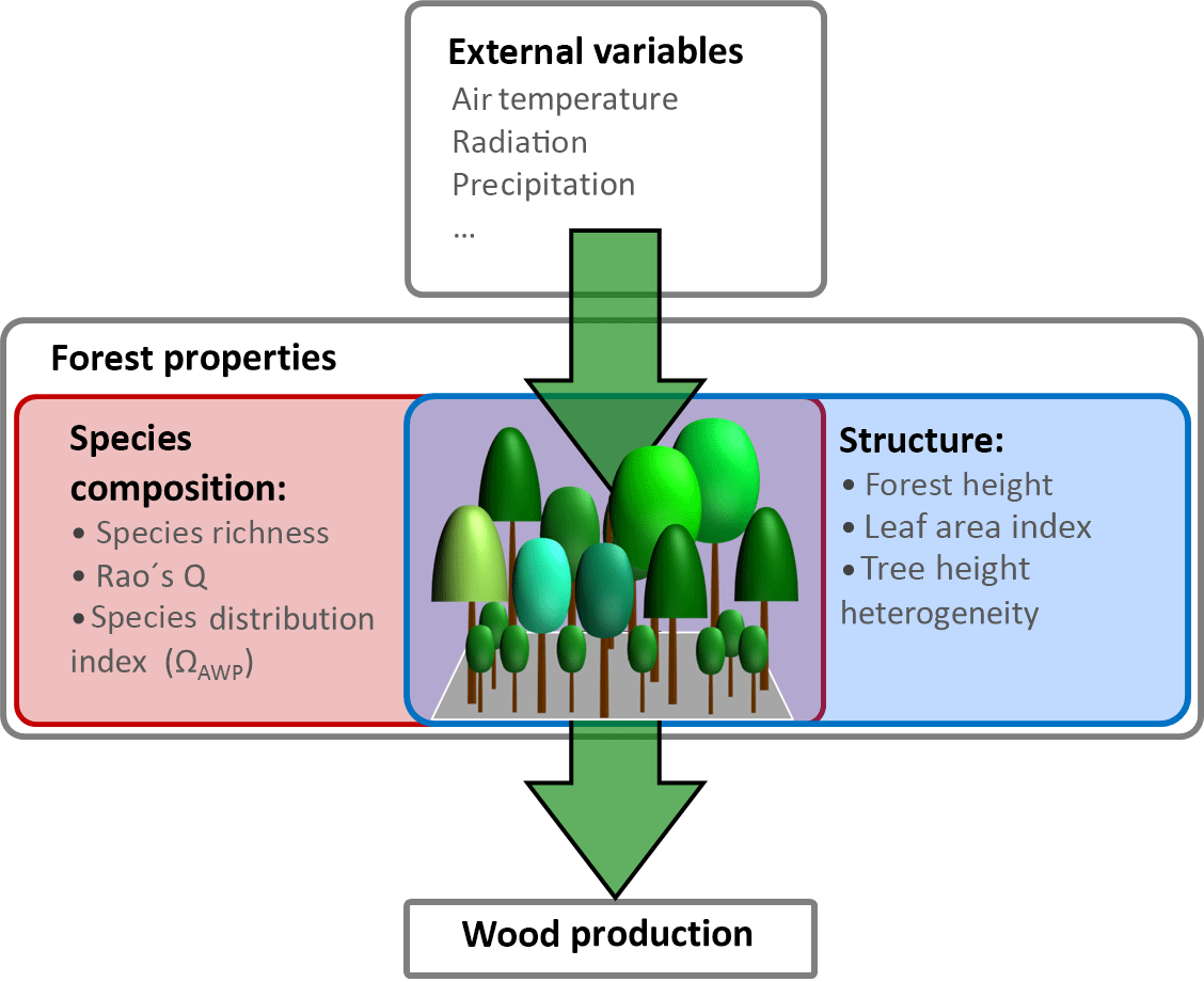
Figure 1Overview of drivers influencing wood production. External variables in this study are temperature, radiation and precipitation. Forest properties are divided into two groups: species composition properties (e.g. Rao's Q as a measure of functional diversity and species distribution index ΩAWP) and forest structure properties (e.g. forest height, leaf area index and tree height heterogeneity).
Forest stands, which differ in their forest properties, might respond differently to the same climate change (Huete, 2016). For instance, the positive effect of increasing temperature on wood production fades with forest age in temperate deciduous forest (e.g. McMahon et al., 2010; Bontemps et al., 2010), and Morin et al. (2014) showed that higher diversity buffers the effect of inter-annual variability on wood production. However, these studies include only a few forest properties and rarely include properties related to both species composition and forest structure. Hence, it is unclear how these forest properties influence wood production change due to temperature rise and which forests will benefit from rising temperatures.
As far as we know, there is no data set available that covers forests, differing in structure and diversity, under almost identical climatic conditions. Even if a larger number of forest stands were available, it would be difficult to manipulate, for instance, temperature while keeping all other climate variables constant. Forest simulation models offer an alternative to the analysis of field experiments. Such models are able to estimate wood production under different climate conditions (e.g. Lasch et al., 2005; Bohn et al., 2014). For instance, Reyer et al. (2014) investigated the effect of climatic change on forests by simulating 30-year time slices of a range of different future climates for 135 inventoried forest stands. There are also model-based studies, which systematically analysed the effect of species diversity on productivity and stability over long periods (Morin et al., 2011, 2014). However, disturbed or managed forest stands and the influence of climate change have not been included in these analyses.
In this study, we therefore propose a new simulation-based approach. First, we generate a large number of forest stands covering various forest structures and species compositions (for up to eight temperate tree species). Annual aboveground wood production (AWP) is then calculated for all forest stands based on climate time series. These time series differ in the mean annual temperature and the intra-annual temperature amplitude. We aim to analyse how productivity of forest stands (AWP) is influenced by (i) increasing mean annual temperature and (ii) increasing intra-annual temperature amplitude. Furthermore, we address the question of which forest stands will benefit most from rising temperatures.
To analyse the effect of temperature on the productivity of forest stands, we applied the “forest factory” model approach (Bohn and Huth, 2017). The forest factory generated 370 170 different forest stands (see Sect. 2.1) and allowed the estimation of AWP under various climate time series (see Sect. 2.2). The 320 scenarios differed in mean annual temperature and annual temperature amplitude. Finally, we calculated the forest-stand-specific sensitivity of productivity to temperature change as the relative change of wood production per temperature change of 1 ∘C (see Sect. 2.2). To relate these sensitivities to forest structure and species composition, we characterized every forest stand with five properties (see Sect. 2.4). We analysed the influence of the five forest properties on temperature sensitivity using boosted regression trees (see Sect. 2.5). Finally, we analysed which combination of forest properties resulted in the highest sensitivity values for different successional stages (see Sect. 2.6). All analysed data are available in the Supplement to this manuscript.
2.1 The forest factory approach
The forest factory creates forest patches based on different stem size distributions and species mixtures. We used 15 stem size distributions covering a gradient from young to old and disturbed to undisturbed forests. Species mixtures included all 256 possible combinations of Pinus sylvestris, Picea abies, Fagus sylvatica, Quercus robur, Fraxinus excelsior, Populus x canadensis, Betula pendula and Robinia pseudotsuga. We used the species parameter set and algorithms of the FORMIND model version for temperate forests within the forest factory (Bohn et al., 2014; Fischer et al., 2016). A total of 100 forest patches of each combination were built.
To generate forest patches, the forest factory randomly chose trees from the stem size distribution, assigned a species identity and planted them within a patch of 400 m2 size. To place a tree within a patch, the following rules must be met: (i) there must be enough space available for crowns of every tree, and (ii) every tree in the forest must have a positive productivity under its environmental conditions (light, temperature, water).
We used climate time series from the year 2007, measured at Hainich National Park, central Germany. We assumed this time series to be a typical example for a temperate year (in principle, it is possible to use climate data from any other location). In contrast to an artificially generated climate, this climate is perfectly physically consistent (with regard to light, air temperature and precipitation).
In a few cases, not all species of the mixture could be placed within a patch by the algorithm, so we rejected such forests. We ended up with 370 100 forest stands. For more details regarding the forest factory, see Bohn and Huth (2017).
2.2 Wood production
The calculation of AWP of trees was based on algorithms of the model FORMIND (Bohn et al., 2014; Fischer et al., 2016). In this model, the wood production of a single tree is calculated as the difference between climate variables driven respiration rates and photosynthesis. The photosynthesis rate (Ptree) results from the crown size, self-shading within the crown and available light at the top of the tree. The available light depends on the radiation above the canopy, reduced by the shading of larger trees within the forest stand. Furthermore, productivity can be limited due to air temperature and available soil water, which is expressed by the photosynthesis-limiting factor ϕ for each tree (Gutiérrez, 2010; Fischer, 2013; Bohn et al., 2014). Available soil water within the stand results from precipitation, interception and evapotranspiration of trees and runoff.
One part of the photosynthesis production of a tree (Ptree) is allocated to its maintenance respiration (and to non-wood tissues; Rm). Maintenance respiration depends on tree biomass and temperature ψ (Piao et al., 2010). The remaining organic carbon is transformed into newly grown aboveground wood (AWPtree) and a proportional growth respiration (rg).
AWPtree was summed over all trees to obtain the productivity of the modelled forest stand – AWP (for a more detailed description of growth processes, see Bohn et al., 2014; Bohn and Huth, 2017).
2.3 Climate sensitivity
To generate a set of 320 annual climate time series, we selected daily climate measurements of the Hainich station in central Germany between the years 2000 and 2004. This time series includes mean daily radiation, precipitation and air temperature (see Appendix A1, Fig. A1). We separated these time series into five distinct time series of 1-year length. First, we increased or decreased the mean annual temperature of each year by adding or subtracting 0.5 ∘C steps between −1.5 and +2 ∘C. Second, we changed the amplitude of the annual temperature cycle for these time series variation of each year. To do so, we modified the standard deviation of each year by 4 % steps between −12 and +16 %. We ended up with five sets of climate time series (of 1-year length) that differ in temperature, precipitation and radiation. Each of these five sets includes 64 time series, which differ only in temperature (see Appendix A1, Fig. A2). Temperature change was quantified using two indices: (i) mean annual temperature and (ii) annual temperature amplitude, which described the 95 % interquartile range of all daily temperature values of a given year. We did not model the effects of nitrogen and CO2 fertilization (as both do not vary strongly within 1 year) or extreme anomalies (e.g. pathogen attacks) on wood production. Figure 2a–c show the AWP for different annual temperatures for three different forest stands.
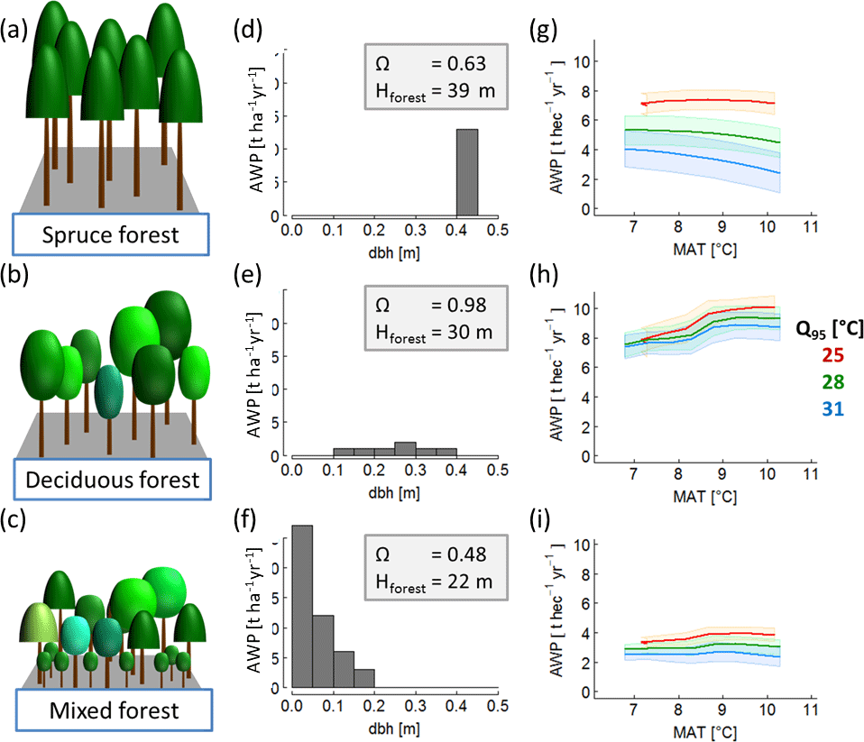
Figure 2Overview of forest properties and resulting temperature sensitivity of AWP of three exemplary forests: (a) old even-aged spruce forest; (b) mature deciduous forest; (c) a quite young mixed species forest. The middle (panels d, e and f) shows the corresponding stem size distributions and provides information on the highest tree in the forest (Hforest) and species distribution index ΩAWP (which quantifies the suitability of a species distributed within the forest structure with regard to AWP). Each forest is treated with 320 climate time series; the last column (panels g, h and i) shows the AWP as a function of mean annual temperature (MAT). The colours indicate different inter-annual temperature amplitudes (Q95) of the used time series. (The coloured bands show the standard deviation due to the variability of the five different time series that exist for each combination of mean annual temperature and intra-annual temperature amplitude.)
We analysed the sensitivity of every forest stand to temperature change following the approach of Piao et al. (2010). For every forest stand, a general linear model was fitted relating wood production mean annual temperature (MAT) and intra-annual temperature amplitude (Q95), as well as the nuisance parameter year.
For every forest, we calculated the relative change of productivity resulting from an increase of 1 ∘C:
In our analysis, we excluded all forests stands for which AWP turns negative if the temperature rises by 1 ∘C (this occurs in 2 % of all stands).
We also determined the sensitivity of forests to temperature change using the German forest inventory to validate our results. However, the inventory does not include leaf area index (LAI) measurements. We therefore assumed the basal area as a proxy for LAI, and we selected subsamples of forests stands with similar structure (basal area, tree height heterogeneity, forest height and same species mixtures). In addition, we used elevation as a proxy for mean annual temperature, assuming temperature changes of 0.65 ∘C per 100 m on average (Foken and Nappo, 2008). Only in the case of spruce and beech monocultures did we find enough data to calculate SIMAT values for several forest structures (for more details, see Appendix A3, Fig. A3).
The comparison between the SIMAT estimation based on the German forest inventory with SIMAT values of corresponding forests from the forest factory showed quite good agreement (R2=0.65). However, the simulated SIMAT values of the forest factory slightly overestimated the sensitivity compared to the inventory-based values (Fig. 3). This might be explained by the difference in the methods used because, in the case of the inventory, we used basal area instead of LAI and altitude instead of temperature. Another explanation could be that in our approach the climate time series showed relatively high and regular precipitation. In the German forest inventory, warmer sites might be more frequently exposed to water stress, which then reduced the SIMAT values.
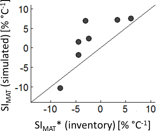
Figure 3SIMAT values of seven different forest types derived from the analysis of the German forest inventory vs. SIMAT values derived from corresponding forest types of the forest factory. Only those SIMAT values of the field data are analysed which showed p values smaller than 0.05.
2.4 Five forest properties to describe forest stands
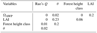
We used three indices to describe the forest structure: LAI, maximum forest height (Hforest), which corresponds to the height of the largest tree in a forest stand, and tree height heterogeneity (θ), which was quantified by the standard deviation of the tree heights. To describe species composition, we used Rao's Q and species distribution index (ΩAWP). Rao's Q quantified functional diversity based on species abundances and differences in species traits (Botta, 2005, for details, see Appendix A2). ΩAWP analysed the optimal location of species within the forest structure. ΩAWP is defined as the ratio of the forest's productivity to the maximum possible productivity of the forest without changing tree sizes or number (Bohn and Huth, 2017). Hence, the maximum productivity can be obtained by varying only the species identities of trees in the forest stand. We changed the assigned species of each tree until we found the optimal species for each individual tree and its specific environmental condition. All five indices were nearly uncorrelated for the investigated forest stands (Appendix A2, Table A1).
2.5 Boosted regression trees
We applied boosted regression trees to quantify the influence of the five forest properties on SIMAT and SIQ95. Boosted regression trees are a machine learning algorithm using multiple decision (or regression) trees. It is able to address unidentified distributions (De'Ath, 2007; Elith et al., 2008). Each model was fitted in a forward stage-wise procedure to predict the response of the dependent variable on (SIMAT or SIQ95) to multiple predictors (tree height heterogeneity, forest height, LAI, Rao's Q and ΩAWP). To omit an overfitting with regard to maximal forest height, we classified forest stands into 18 classes. Each class had a width of 2 m, starting with 4 to 6 m and finishing with 36 to 38 m. The boosted regression trees tried an iterative process to minimize the squared error between predicted SI values and those of the data set. Hereby, part of the data were used for a fitting procedure and the rest was used for computing out-of-sample estimates of the loss function (Ridgeway, 2015). This boosted regression tree analysis was performed in the R package gbm 2.1.1 (Ridgeway, 2015).
We used a quarter of the data (randomly sampled) for the machine learning procedure. To get the best model, we varied the following four parameters of the boosted regression tree algorithm: learning rates (0.1, 0.05 and 0.01), the bag fractions (0.33, 0.5 and 0.66), the interaction depths (1, 3 and 5) and the cross validation (3-, 6- and 9-fold) assuming a Gaussian error structure (the default setting). The best-fitted boosted regression tree for both SIMAT and SIQ95 showed a learning rate of 0.1, a bag fraction of 0.66, an interaction depth of 5 and a 3-fold cross validation. These two models were used for all further analyses. The remaining 75 % of the data were used to validate the fitted boosted regression tree algorithm.
2.6 Finding the forest stands for different successional stages that benefit the most increasing temperatures
Here, we assumed forest height as a proxy for the successional stage of a forest. In every height class, we selected those 5 % of forests that showed the highest sensitivity values (SIMAT and SIQ95). We removed the forest height classes between 10 and 14 m, as they only contained only 15 forests. For all other classes, we analysed the relationship between height class and the forest properties (ΩAWP, Rao's Q, LAI and tree height heterogeneity).
We analysed the sensitivity of productivity (AWP) to temperature for forest stands that differ in forest properties (species distribution index (ΩAWP), functional diversity (Rao's Q), tree height heterogeneity (θ), forest height class and LAI). The annual AWP was estimated for each forest stand using 320 different climate time series. We then quantified the changes in productivity resulting from changes in mean annual temperature (SIMAT) and intra-annual amplitude (SIQ95). For the analysed forest stands, the average SIMAT is 1.5 % ∘C−1 and the average SIQ95 is −5.4 % ∘C−1 (see also the frequency distribution in Appendix B1, Fig. B1).
With a boosted regression tree algorithm, we analysed how the five forest properties influence the temperature sensitivity of forests. To validate the fitted boosted regression tree algorithm, we compared SI values, which are not used for the fitting, with the SI value predicted by the boosted regression tree algorithm (Fig. 4). The sensitivities to mean annual temperature change (SIMAT) correlated very well (R2 of 0.84) and showed a low root mean squared error (RMSE) of ±2.9 % ∘C−1 (see Appendix B2, Fig. B3). The RMSE even decreased to ±1.5 % ∘C−1 if a subset of the forest stands was analysed that showed SIMAT values larger than −5 % ∘C−1 (90 % of the data). The accuracy of the sensitivities to temperature amplitude change (SIQ95) was even slightly better. In addition, a subset that included SIQ95 values larger than −15 % ∘C−1 (93 % of the data) showed a RMSE of only ±1.1 % ∘C−1 (see Appendix B2, Fig. B4).
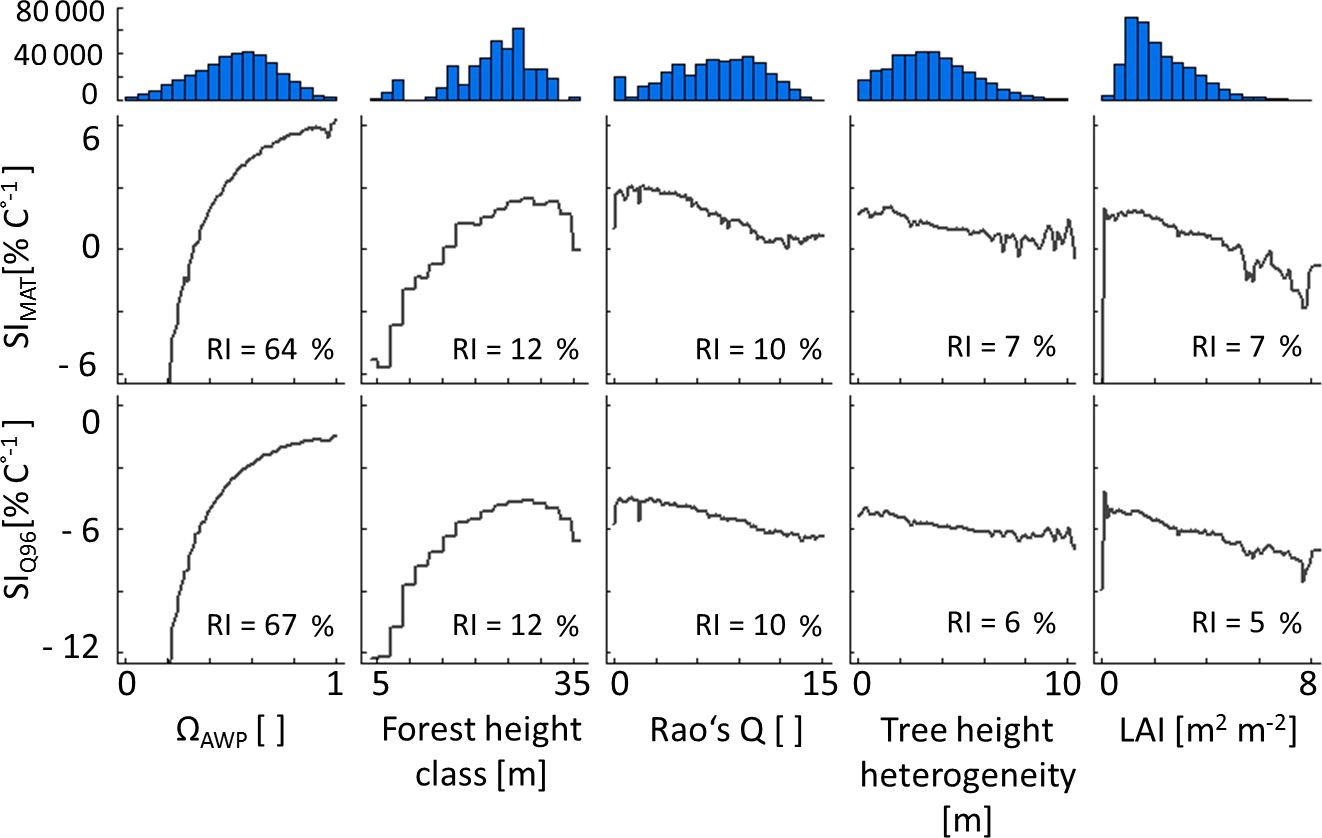
Figure 4Partial dependency plots of the five forest properties – ΩAWP (species distribution index), forest height class, Rao's Q (functional diversity), tree height heterogeneity and LAI (leaf area index) – for SIMAT (sensitivity to changes in the mean annual temperature) and SIQ95 (sensitivity to changes in annual temperature amplitude). Relative importance (RI) compares the influence of different input variables on the variability of a target variable. Histograms show the frequency of forest property values in the analysed data set. Note that ΩAWP is the ratio of the current AWP of a forest and the highest possible AWP obtained by shuffling only species identities without changing the forest structure.
According to boosted regression tree analysis, ΩAWP was the most relevant forest property to explain temperature sensitivities (relative influence of 87 % for SIMAT and 89 % for SIQ95; see also Appendix B2, Fig. B2). However, the influence of ΩAWP on temperature sensitivity flattened out for high ΩAWP levels (Fig. 5). The second relevant forest property was forest height (Hforest). Forests with heights between 25 and 30 m benefited the most from increasing mean annual temperatures. The other three properties (LAI, Rao's Q and tree height heterogeneity) had a low influence on SIMAT.
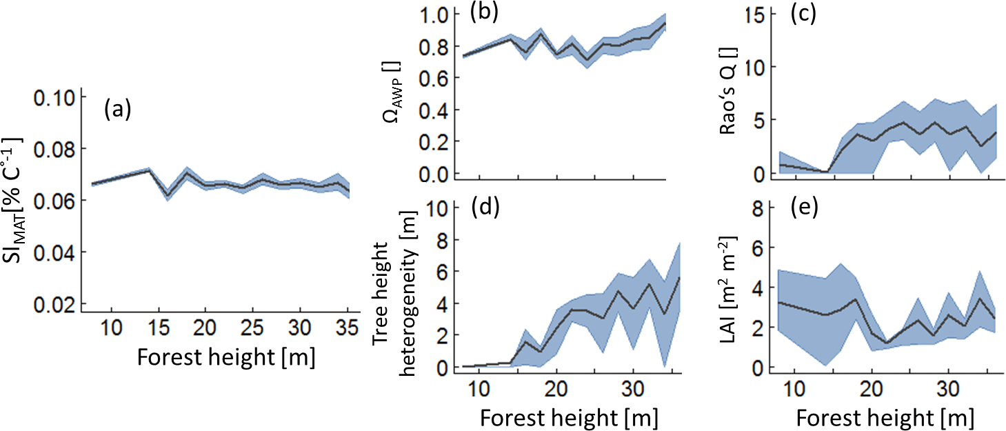
Figure 5Analysis of those forests that show the highest 5 % of the SIMAT values depending on forest height. Lines indicate mean values of the forest subsamples which include the best 5 % with regard to SIMAT of each hight class. The grey band indicates the interquartile range. Panel (a) shows temperature sensitivity of aboveground wood production over forest height, analysing only the best the forest subsample. Panels (b) to (e) show the change of the remaining forest properties within the forest subsamples (ΩAWP is the optimal species distribution; LAI is the leaf area index; Rao's Q quantifies functional diversity).
Both sensitivity indices showed similar relationships to the five forest properties. However, an increase in annual temperature amplitude always reduced productivity, whereas increasing mean annual temperature could result in a positive effect on wood production. To detect those stands that benefit the most from increasing temperature, we selected the 5 % of forest stands that showed the highest SIMAT values in each forest height class (Fig. 5). In all forests classes, we found forest stands that would benefit from increasing temperatures. Analyses of their forest properties revealed that the ΩAWP levels were always high. Young forests (low forest height), which had a positive temperature sensitivity, showed low functional diversity and low tree height heterogeneity (θ). For older forests (of intermediate and high forest height) with positive temperature sensitivity, we found an intermediate level of functional diversity. Interestingly, for three variables (Rao's Q, tree height heterogeneity and LAI), the relationships changed their character between young and intermediate forest heights. We obtained similar simulation patterns for SIQ95 (Appendix B3, Fig. B5).
3.1 Understanding the patterns
3.1.1 The influence of forest structure on temperature sensitivity
Forest structure affects the wood production of single trees in two ways. First, it determines the amount of light available to each individual tree, and second, the size of trees influences their photosynthesis and respiration rates (Fig. B6). Hence, based on the height of a tree and the amount of light available to it, it was possible to calculate its SI values (for a detailed discussion of these calculations, see Appendix B4).
In even-aged forests, all trees have the same height and receive full light (e.g. Fig. 6; forest C). In our study, such forests showed a bell-shaped relationship between forest height and temperature sensitivity (Fig. 6; SI values for 100 % available light depending on tree height).
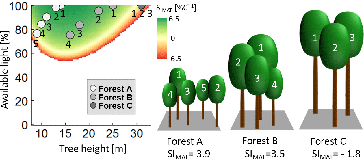
Figure 6Analysis of the sensitivity index of AWP against mean annual temperature (SIMAT) values of single trees within three different forests. The diagram shows the calculated SIMAT value of individual trees for every combination of tree height and available light (for Pinus sylvestris between SIMAT levels of 6.5 and −6.5; other species show similar patterns). The dots indicate the different trees of the three forest examples. The white dots belong to trees with the corresponding number of forest A, grey dots belong to the trees of forest B, and dark grey dots belong to forest C. Note that, in the case of forest C, all trees have the same height and the same light, so that all three dots are at the same place in the diagram.
In the case of a forest consisting of trees of different heights, smaller trees receive less light due to shading. Note that, even if trees received less light, the bell-shaped relationship between tree height and productivity persisted (Fig. 6). Two cases will be discussed (assuming identical LAI as forest C; Fig. 6). In the first case, all trees have not yet reached their maximal SI values (Fig. 6; forest A); in the second case, all trees have already passed their maximal SI values (Fig. 6; forest B). In the case of forest A, trees in the shade of larger trees always had lower SI values if they belonged to the same species (see Appendix B4). Hence, the temperature sensitivity level of this forest was lower than the sensitivity of an even-aged forest, whose trees have the same size as the largest tree in forest A (Fig. 6; tree 1). Hence, if maximal SI values were not reached, increasing height heterogeneity decreased SI values of a forest.
In forest B (Fig. 6), SI values of the shaded trees can be similar (or even higher) than the SI value of the largest trees in the forest (SI values of tree 1 show similar levels to trees 2, 3 and 4 in forest B; Fig. 6). Hence, if maximal SI values were passed, increasing tree height heterogeneity resulted in similar (or even more positive) temperature sensitivity levels compared to even-aged forest trees (an even-aged forest consisting only of trees similar to tree 1 of forest B in Fig. 6). These general considerations explain the change from low levels of height heterogeneity in young forests to a more heterogeneous structure in the analysis of those forests, which will benefit from increasing temperature (see Fig. 5d).
3.1.2 The effect of species composition on temperature sensitivity
In this study, we use the new ΩAWP index called the species distribution index (Bohn and Huth, 2017). ΩAWP is the ratio between current AWP and the highest possible AWP of the forest which can be reached due to shuffling of species identities. Its huge importance for forest temperature sensitivity might be illustrated by the following considerations. If species are unfavourably distributed within the forest (low ΩAWP), the AWP of the forest is low.
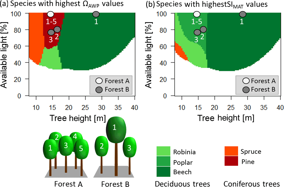
Figure 7Panel (a) shows which species have the highest productivity (ΩAWP value of 1) under the current climate for different heights and different light conditions. Panel (b) shows which species show the highest increase in productivity due to rising temperatures for different heights and different light conditions. Red colours indicate coniferous trees, whereas green colours indicate deciduous trees. Darker colours indicate late successional species, whereas lighter colours indicate pioneers. The dots indicate the different trees of the two forest examples (A and B). The white dots belong to trees with the corresponding number of forest A. Note that all trees have the same height and the same light, so all five dots are at the same place in the diagram. Grey dots belong to the corresponding trees with the same number of forest B.
Increasing functional diversity (Rao's Q) stabilized the forests' sensitivity to temperature. This corresponds to results of Morin et al. (2014) and the theoretical consideration of Yachi and Loreau (1999). The analysis of the single species can give additional insight into the mechanisms behind those species that benefited the most from temperature increase, which were deciduous trees under most conditions. This is reasonable as warmer regions host more deciduous species than needleleaf species. The highest functional diversity (Rao's Q), on the other hand, occurred in mixtures of deciduous and needleleaf trees (Appendix B5, Fig. B7). As only two needleleaf species were considered here in the species pool, low Rao's Q values were dominated by mixtures of deciduous trees. Such deciduous tree mixtures mostly benefited from temperature increases. In contrast, mixtures with high Rao's Q values, which mostly included both functional types, reacted more poorly (Fig. 4; Appendix B5, Fig. B7).
We developed two diagrams that show the species with the highest temperature sensitivity and with the highest productivity for different conditions (available light and height of a tree) (Fig. 7). Interestingly, the species with the highest productivity differed from the species that benefit most from rising temperatures in many cases. This has important implications. The highest benefit due to increasing temperatures was obtained by forests with high but not maximal ΩAWP (Fig. 5). Additionally, deciduous trees benefited more than coniferous trees from rising temperatures (Fig. 7, Appendix B5, Fig. B7). Hence, young forests should consist of deciduous trees (compare Figs. 6 and 7; forest A), although the highest productivity values are found for coniferous trees (Fig. 7; forest A). Forests including large trees obtained the highest sensitivity values if intermediate-sized trees differed in their species identity from the largest trees (Fig. 7).
4.1 The study design
In this theoretical study, we present a new climate sensitivity analysis (with regard to temperature) of AWP. This approach extends field observations and long-term model simulations, as it allows the analysis of existing forests but also of those that might exist in the future due to management changes and/or disturbances. Our approach includes only forest stands in which every tree has positive productivity and enough space for its crown. Hence, it is impossible, for instance, that light-demanding species grow below a closed canopy or forests are overcrowded. However, the data set also includes a few very unusual stand structures or species combinations, which cannot emerge in a natural system, but may result from disturbances or management. In the case of field observations, it is difficult to explore the influence of a single climate variable (e.g. temperature) on one target variable (e.g. AWP), as in most cases, several variables are altered at the same time (see also Appendix A3). Process-based models are one option to analyse such relationships and separate these effects. The simulation of AWP with the FORMIND model in temperate forests has been successfully compared to eddy flux sites (Rödig et al., 2017b), the national German forest inventory (Bohn and Huth, 2017) and European yield tables (Bohn et al., 2014).
An advantage of the forest factory approach is the huge set of various forests stands that can be analysed. The data set includes forest stands that often occur in temperate forests (even-aged spruce, pine and beech stands). However, it also includes hypothetical ones that could occur through alternative forest management or disturbances (fire, bark beetles, etc.). Hence, our data set of forest stands covers a much larger variety of forest property combinations compared to long-term forest simulations with the focus on natural forests in their equilibrium state (e.g. Morin et al., 2011) or on monocultures (e.g. Reyer et al., 2014). Long-term simulations with ecosystem models, which process modelled climate projections, face a trade-off between cascade uncertainty and path dependency (Wilby and Dessai, 2010; Reyer et al., 2014). The accumulations of model uncertainties over such a process chain result in increasing uncertainty. Our study design tries to minimize this uncertainty and omit path dependencies by including only those processes that might be relevant for the research question. In this study, for instance, we omit the effect of climate change on regeneration and mortality. Furthermore, using several climate variables as model inputs but only analysing the effect of one variable might lead to incorrect interpretations of its effect. For example, temperature and radiation often correlate, and both might increase productivity. Therefore, in this study, we only vary one variable in all five sets of time series. This guarantees that there are no relationships between the target climate variable and the remaining climate variables.
As an increase in global mean temperature of 1.5 to 2 ∘C can hardly be avoided, even under the Representative Concentration Pathway (RCP) 2.6 climate scenario (IPCC, 2013), this study focuses on temperature change. This RCP scenario predicts only small changes in annual precipitation levels for temperate regions. Hence, our approach focuses only on the effect of temperature change on wood production. However, this might be critical for the analysis of strong temperature changes (e.g. RCP8.5) which will result in an increased incidence of drought and changes in the annual temperature cycles and a strong change in CO2. Such more complex scenarios should be analysed in future studies. Further, we neglect the effect of time lags (e.g. bud building in the previous year). However, it is possible to extend the used time series to analyse the behaviour of the forest over longer time periods and study not only productivity but also effects on regeneration or mortality.
To characterize the annual temperature cycles, we used two variables: mean annual temperature and intra-annual temperature amplitude. Both variables can be varied independently. In the case of higher mean annual temperature, we observe an elongation of the vegetation period. This leads to higher forest productivity (if other resources are not limiting (Luo, 2007) and explains why SIMAT is often positive. However, warmer summer temperatures can also lead to a decline in wood production due to an increase in respiration. In the case of increasing intra-annual temperature amplitude, more days with extreme temperatures will occur in a year. Thus, an increase of 1 ∘C−1 of intra-annual temperature amplitude will increase respiration more strongly compared to an increase of 1 ∘C−1 of mean annual temperature. Hence, the increase of intra-annual temperature amplitude normally has negative effects on the productivity (negative SI values).
The temperature sensitivity values obtained here are in the same range as those found for temperate ecosystems in heating experiments (Lu et al., 2013, 4.4 ± 2.2 % ∘C−1). Within the 16 analysed studies reviewed by Lu et al. (2013), the experimental plots show almost identical environmental conditions (soil, radiation and precipitation) and species composition. To heat the plots, greenhouses or infrared heaters were used. Another study, based on natural forest stands in New Zealand, found an AWP increase of between 5 and 20 ∘C−1 for forests, assuming no change in forest structure and species composition (Coomes et al., 2014). The analysed plots were spread throughout New Zealand, and warmer temperatures coincided with higher radiation (Mackintosh, 2016). Hence, the analysed temperature effect also includes the influence of radiation. In our setting, however, the influence of temperature is independent of radiation (Lu et al., 2013, as in). We also found a good correlation between SI values derived from growth measurements of the German forest inventory and simulated SI values based on the forest factory (Fig. 3, Appendix A3, Fig. A3).
4.2 Implications for forest management
Our findings might be relevant for future management strategies for temperate forests. Specifically, our new understanding of which species benefit most from rising temperatures (Fig. 6) suggests possible strategies, e.g. replacing spruce monocultures with mixtures of deciduous trees. Further, based on the analysis of which forest structure benefits most from rising temperatures (Figs. 4, 5, 6), early-stage even-aged forests should include mainly pioneer species. In the mature stage, we predict a positive effect of temperatures on wood production for a mixture of climax species including different tree sizes. These climax species could be planted below the canopy of the pioneer species in young forests. In our approach, we do not simulate the establishment of very young trees. However, during the conversion between these two forest types, one big challenge might be the removal of the pioneer trees without damaging the young trees that will build the mature forest.
4.3 Implications for global vegetation modelling
Most global vegetation models represent vegetation as fractional cover of different plant functional types within a grid cell (e.g. Lund–Potsdam–Jena (LPJ); Sitch et al., 2003). Only a few global vegetation models include a more detailed representation of vegetation structure and functional diversity (Sato et al., 2007; Scheiter et al., 2013; Sakschewski et al., 2016). It would be interesting to perform the analysis presented here with global vegetation models which include structure to better understand the mechanisms driving forest systems' sensitivity to climate change.
Besides the global vegetation models, forest gap models, which have been restricted to local stands, are now able to simulate forest dynamics in regions or even entire continents (Seidl and Lexer, 2013; Rödig et al., 2017a). Studies using global vegetation models or large-scale forest gap models simulate natural succession. Our analysis indicates that natural and managed (or disturbed) forest systems, which differ in forest structure, might react differently to climate change. Hence, we suggest considering forest structure in future analyses of global vegetation. Such information on forest structure might be derived from remote sensing.
The temperature sensitivity of wood production in temperate forests is influenced by forest structure and species diversity as our study showed. The species distribution index (ΩAWP) and forest height seem to be the most important forest properties influencing temperature sensitivity.
Temperate forests that benefit most from temperature rise are those which consist of even-aged deciduous pioneer species in the case of young forests; mature forests benefit most if tree height heterogeneity is large and the forest includes different deciduous climax species.
This study also attempts to explain why certain forest types will decrease their productivity and others will not. Our findings highlight the importance of forest structure for future studies investigating wood production under climate change.
The R workspace which includes the data set of the analysed forests (“foreststands”) and the calculated SI values (“SIValues”) can be found in the Supplement to this paper.
A1 Climate data
The construction of the 320 climate time series is based on measured climate time series of the eddy flux Hainich station in central Germany (Knohl et al., 2003) for the years 2000–2004 (Fig. A1). Mean annual temperature of these 5 years does not correlate with the annual precipitation sum, nor with the mean annual radiation (Fig. A2). Radiation and precipitation within these years correlate quite well (Pearson's r=0.73).
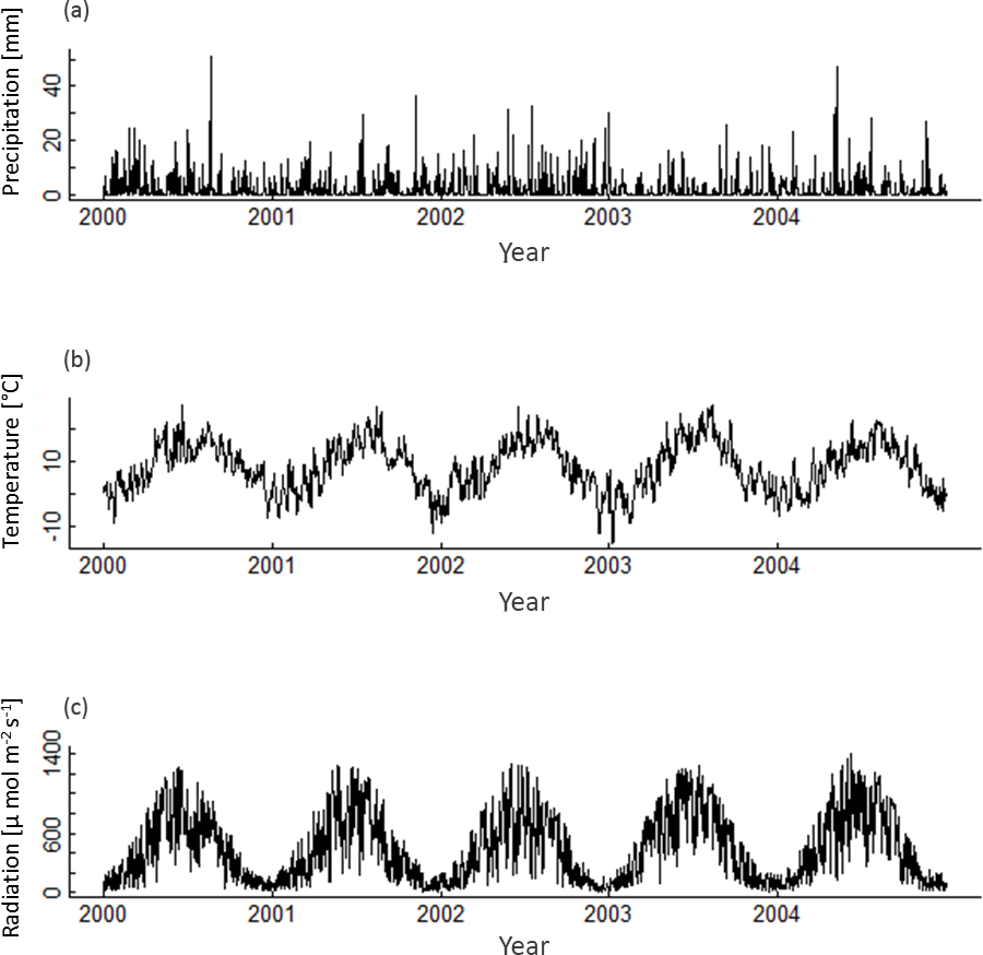
Figure A1The climate time series measured at FLUXNET Hainich station from 2000 to 2004 which are used to generate the 320 climate time series: (a) daily precipitation (mm), (b) daily air temperature (% ∘C−1), (c) daily incoming radiation (photoactive photon flux density, ).
A2 Forest properties
We use three forest properties to describe forest structure (tree height heterogeneity (θ), forest height class and LAI) and two properties to describe species diversity (Rao's Q describes functional diversity and ΩAWP describes suitability). The calculation of Rao's Q is based on 12 species-specific parameters which are relevant for productivity (AWP) and species abundance (based on crown area). None of the properties correlate (Table A1).
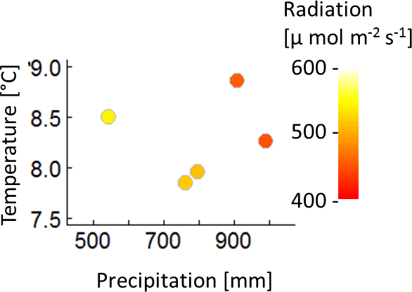
Figure A2Mean annual temperature, annual precipitation sum and mean annual radiation of the five climate time series measured at Hainich station from 2000 to 2004.
Table A1Coefficient of determination (R2) between all used internal forest properties for 370 170 stands of the forest factory. θ is the tree height heterogeneity; LAI is the leaf area index; ΩAWP is the species distribution index.
A3 Validation with the German forest inventory
We analysed the influence of forest structure on temperature sensitivity within the German forest inventory (beech monocultures and spruce monocultures. Tree height was used to calculate forest height (Hforest) and tree height heterogeneity (θ). We replaced LAI, which is not measured, by basal area (both properties correlate quite well in the forest factory data set; R2=0.74). The forest stands of each species were classified into six structure classes: three classes which are based on the height of the largest tree in the forest stand (10–15, 20–25 and 30–35 m) and two classes representing different tree height heterogeneities (0–1 and >1.6 m). Only plots that are located on flat terrain (slope of less than 15 %) and have a maximum stem diameter of 0.5 m) were analysed. A linear model was fitted to the data of every class using basal area and elevation as input variables to predict AWP.
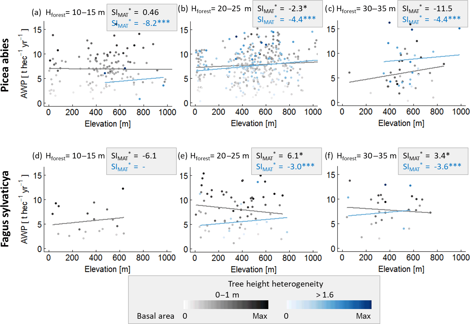
Figure A3Analysis of the influence of forest structure on the relationship between elevation and AWP. Panels (a)–(c) are based on spruce monocultures and (d)–(f) on beech monocultures. For each species, forest stands were classified into three forest height classes which were based on the largest tree (Hmax) in a forest stand. These forest stand classes were additionally separated into two tree height heterogeneity classes (0–1 m in grey and >1.6 m in blue). Intensities of the colours indicate the ratio between basal area of the stand and maximal basal area found within one class. Lines show the results of the linear model with mean basal area. The amount of stars behind the SI values indicates the significance of the slope within a linear model: indicates a p value below 0.001, and (*) indicates a p value between 0.01 and 0.05. Absence of stars indicates p values above 0.1. The unit of SI is % ∘C−1.
B1 Frequency distribution of sensitivity values
The analysed forest stands show a large range of temperature sensitivity levels, which reach up to 8.5 % ∘C−1 in the case of SIMAT (Fig. B1a). This means that one forest increases its productivity by 8.5 % due to an increase in the mean annual temperature of 1 ∘C. In the case of the annual temperature amplitude, the best forest reduces its productivity by −0.5 % ∘C−1 (Fig. B1b). The mean SIMAT is 1.5 % ∘C−1 and the interquartile range (iqr) ranges from 1.6 to 5.2 % ∘C−1. The mean SIQ95 is −5.4 % ∘C−1 and the iqr ranges from −5.2 to −2.2 % ∘C−1.

Figure B1Frequency distribution of SIMAT values (a) and SIQ95 values (b) of all forest stands.
B2 Analysis with boosted regression trees
Boosted regression trees provide information about the underlying relationship between input variables (here forest properties) and output variables (here SI values). Several techniques were developed to visualize and interpret the high-dimensional relationship of input and target variables (Friedman, 2001). The comparisons between SI values of the forest factory and predicted SI values (based on the five properties as input), show a very high agreement (Figs. B2 and B3). The obtained vertical patterns for SIMat (0) and SIQ95 (−6 % ∘C−1) are probably artefacts of the boosted regression tree algorithm.
Other commonly used visualizations of the relationship of input and target variables are partial dependency plots (Fig. 4). These plots show the influence of an input variable on the target variable considering the influence of all input variables which have higher relative importance. In our study, the most important variable is ΩAWP; hence, the first plot shows the relationship between suitability and SI values. The second relationship (forest height and SI values) is based on the residuals of the first relationship (here between SI values and ΩAWP; Becker et al., 1996). Although a collection of such plots can seldom provide a comprehensive analysis of the boosted regression trees, it can often produce helpful hints, especially if variables show very low correlations, as in this study.
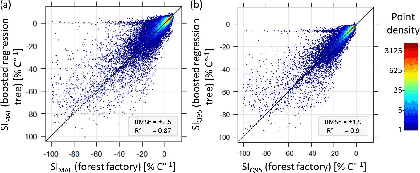
Figure B2Comparisons of temperature sensitivity (SIMAT and SIQ95) based on the forest factory and boosted regression tree model. Colours indicate point density. Diagonal is the 1:1 line.
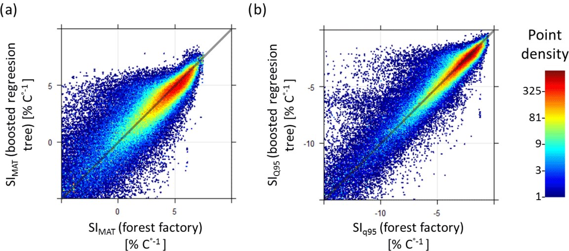
Figure B3Comparison of temperature sensitivity calculations (SIMAT and SIQ95) based on the forest factory and boosted regression tree model. Colours indicate point density. Diagonal is the 1:1 line. Panel (a) contains 90 % of the forest factory data set and (b) contains 93 % of the forest factory data set.
Forest stand properties with highest SIQ95 values over a forest height gradient
The analysis of those forests, which lie above the 95th percentile of SIQ95, depending on forest height, shows almost the same pattern as the identical analysis of SIMAT (compare Fig. B4 with Fig. 5).
B4 SI values of single trees
To understand the origin of the SI values, we make the following assumptions. An increase of 1 % ∘C−1 always results in an increase of 8.6 % of the respiration rate in the model (Fig. B5b; Piao et al., 2010). The positive effect of a temperature increase of 1 % ∘C−1 on the photosynthesis rate varies between the years due to the assumed species-specific bell-shaped relationship (Fig. B5a). In the case of deciduous trees, the length of the vegetation period (leaf onset to fall) additionally affects the annual photoproduction (e.g. Haxeltine and Prentice, 1996; Luo, 2007; Horn and Schulz, 2011; Gutiérrez and Huth, 2012; Sato et al., 2007). If the photosynthesis rate is much larger than the respiration rate (high AWP; for instance, low ratio of maintenance respiration to photosynthesis under full light in Fig. B6b), the positive effect of temperature on photosynthesis causes an increase of AWP in some simulated years. If both rates show the same magnitude (ratio of maintenance respiration to photosynthesis under full light is close to 1 in Fig. B6b), higher temperatures increase respiration more than photoproduction (in most years), which results in a decrease of AWP.
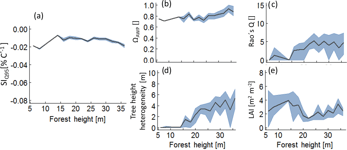
Figure B4Analysis of those forests which lie above the 95 % percentile of SIQ95, depending on forest height Hforest. Lines indicate mean values of the subsamples and the grey bands indicate the interquartile range. Panel (a) shows the temperature sensitivity of productivity to forest height, analysing only values above the 95 % percentile; (b) to (e) show the change of the remaining forest properties within the subsamples.
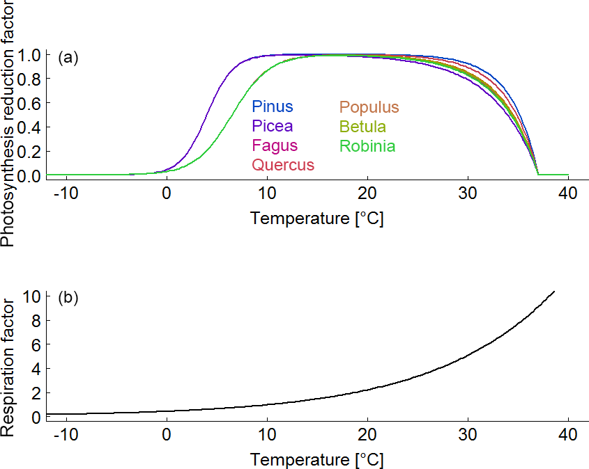
Figure B5(a) Species-specific reduction factor of photosynthesis due to a change in air temperature. (b) Species-unspecific correction factor for maintenance respiration due to a change in air temperature.
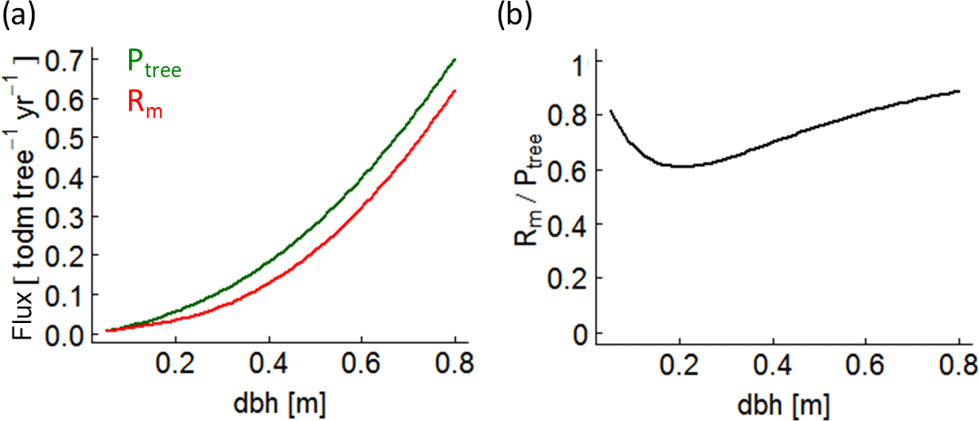
Figure B6(a) Photosynthesis (green line – Ptree) and maintenance respiration (red line – Rm) rates of a single beech tree over stem diameter (dbh) under full light. (b) The ratio between maintenance respiration and photosynthesis of the same beech tree.

Figure B7Rao's Q (with equal abundances) against values of all possible species mixtures (from the forest factory). The values are the average over all SIMAT values for all light–height combinations and with values larger than −7.5 % ∘C−1. For mixtures, we assumed equal abundances and calculated the mean over the SIMAT values of all species within the mixture. Green dots indicate forests that consist only of deciduous trees; red dots indicate forests that consist only of needleleaf trees; blue dots indicate forests that contain both tree types.
B5 Functional diversity and temperature sensitivity
To analyse the effect of functional diversity on temperature sensitivity, we first calculated SIMAT for every species depending on tree height and light availability (as done for pine trees in Fig. 6). Then, we calculated a mean SIMAT value for each species mixture for all light–height combinations. Finally, we averaged those SI values which were larger than −7.5 % ∘C−1 () and calculated the Rao's Q of the mixtures (based on equal abundances). The highest values were found for deciduous forests (Fig. B7). Mixed forests with deciduous and needleleaf trees showed lower values than the deciduous forests but higher Rao's Q values.
The supplement related to this article is available online at: https://doi.org/10.5194/bg-15-1795-2018-supplement.
FJB, FM and AH conceived of the study. FJB implemented and analysed the simulation model and wrote the first draft of the manuscript. AH and FM contributed to the text. All authors gave their final approval for publication.
The authors declare that they have no conflict of interest.
We thank Edna Rödig, Franziska Taubert, Nikolaj Knapp, Rico Fischer and Kristin Bohn for providing many helpful suggestions and comments.
We also thank the Department of Bioclimatology of the University of Göttingen
and the Max Planck Institute of Biogeochemistry for providing climate data
and the administration of Hainich National Park for permission to conduct
research there.
The article processing charges for this open-access
publication were covered by a Research
Centre of the Helmholtz Association.
Edited by: Sebastiaan Luyssaert
Reviewed by: Christopher Reyer and one anonymous referee
Asner, G. P., Scurlock, J. M., and A Hicke, J.: Global synthesis of leaf area index observations: implications for ecological and remote sensing studies, Global Ecol. Biogeogr., 12, 191–205, https://doi.org/10.1046/j.1466-822X.2003.00026.x, 2003. a
Barber, V. A., Juday, G. P., and Finney, B. P.: Reduced growth of Alaskan white spruce in the twentieth century from temperature-induced drought stress, Nature, 405, 668–673, https://doi.org/10.1038/35015049, 2000. a, b
Barford, C. C., Wofsy, S. C., Goulden, M. L., Munger, J. W., Pyle, E. H., Urbanski, S. P., Hutyra, L., Saleska, S. R., Fitzjarrald, D., and Moore, K.: Factors controlling long-and short-term sequestration of atmospheric CO2 in a mid-latitude forest, Science, 294, 1688–1691, https://doi.org/10.1126/science.1062962, 2001. a
Becker, R. A., Cleveland, W. S., and Shyu, M.-J.: The visual design and control of trellis display, J. Comput. Graph. Stat., 5, 123–155, 1996. a
Bohn, F. J. and Huth, A.: The importance of forest structure to biodiversity-productivity relationships, Roy. Soc. Open Sci., 3, 160521, https://doi.org/10.1098/rsos.160521, 2017. a, b, c, d, e, f, g
Bohn, F. J., Frank, K., and Huth, A.: Of climate and its resulting tree growth: Simulating the productivity of temperate forests, Ecol. Model., 278, 9–17, https://doi.org/10.16/j.ecolmodel.2014.01.021, 2014. a, b, c, d, e, f
Boisvenue, C. and Running, S. W.: Impacts of climate change on natural forest productivity–evidence since the middle of the 20th century, Glob. Change Biol., 12, 862–882, https://doi.org/10.1111/j.1365-2486.2006.01134.x, 2006. a
Bonan, G. B.: Forests and Climate Change: Forcings, Feedbacks, and the Climate Benefits of Forests, Science, 320, 1444–1449, https://doi.org/10.1126/science.1155121, 2008. a
Bontemps, J.-D., Hervé, J.-C., and Dhôte, J.-F.: Dominant radial and height growth reveal comparable historical variations for common beech in north-eastern France, Forest Ecol. Manag., 259, 1455–1463, https://doi.org/10.1016/j.foreco.2010.01.019, 2010. a, b
Botta-Dukát, Z.: Rao's quadratic entropy as a measure of functional diversity based on multiple traits, J. Veg. Sci., 16, 533–540, https://doi.org/10.1111/j.1654-1103.2005.tb02393.x, 2005.
Charru, M., Seynave, I., Morneau, F., and Bontemps, J.-D.: Recent changes in forest productivity: an analysis of national forest inventory data for common beech (Fagus sylvatica L.) in north-eastern France, Forest Ecol. Manag., 260, 864–874, https://doi.org/10.1016/j.foreco.2010.06.005, 2010. a
Coomes, D. A., Flores, O., Holdaway, R., Jucker, T., Lines, E. R., and Vanderwel, M. C.: Wood production response to climate change will depend critically on forest composition and structure, Glob. Change Biol., 20, 3632–3645, https://doi.org/10.1111/gcb.12622, 2014. a
De'Ath, G.: Boosted trees for ecological modeling and prediction, Ecology, 88, 243–251, https://doi.org/10.1890/0012-9658(2007)88[243:BTFEMA]2.0.CO;2, 2007. a
Delpierre, N., Soudani, K., Francois, C., Köstner, B., Pontailler, J.-Y., Nikinmaa, E., Misson, L., Aubinet, M., Bernhofer, C., Granier, A., Heinesch, B., Longdoz, B., Ourcival, J.-M., Rambal, S., Vesala, T., and Dufrên E.: Exceptional carbon uptake in European forests during the warm spring of 2007: a data–model analysis, Glob. Change Biol., 15, 1455–1474, https://doi.org/10.1111/j.1365-2486.2008.01835.x, 2009. a
De Vries, W., Reinds, G. J., Gundersen, P., and Sterba, H.: The impact of nitrogen deposition on carbon sequestration in European forests and forest soils, Glob. Change Biol., 12, 1151–1173, https://doi.org/10.1111/j.1365-2486.2006.01151.x, 2006. a
De Vries, W., Solberg, S., Dobbertin, M., Sterba, H., Laubhann, D., Van Oijen, M., Evans, C., Gundersen, P., Kros, J., Wamelink, G., Reinds, G. J., and Sutton, M. A.: The impact of nitrogen deposition on carbon sequestration by European forests and heathlands, Forest Ecol. Manag., 258, 1814–1823, https://doi.org/10.1016/j.foreco.2009.02.034, 2009. a
Dillon, M. E., Wang, G., and Huey, R. B.: Global metabolic impacts of recent climate warming, Nature, 467, 704–706, https://doi.org/10.1038/nature09407, 2010. a
Elith, J., Leathwick, J. R., and Hastie, T.: A working guide to boosted regression trees, J. Anim. Ecol., 77, 802–813, https://doi.org/10.1111/j.1365-2656.2008.01390.x, 2008. a
Fischer, R.: Modellierung der dynamic afrikanischer Tropenwälder, Ph.D. thesis, Universität Osnabrück, 2013. a
Fischer, R., Bohn, F., de Paula, M. D., Dislich, C., Groeneveld, J., Gutiérrez, A. G., Kazmierczak, M., Knapp, N., Lehmann, S., Paulick, S., Pütz, S., Rödig, E., Taubert, F., Köhler, P., and Huth, A.: Lessons learned from applying a forest gap model to understand ecosystem and carbon dynamics of complex tropical forests, Ecol. Model., 326, 124–133, https://doi.org/10.1016/j.ecolmodel.2015.11.018, 2016. a, b
Foken, T. and Nappo, C. J.: Micrometeorology, Springer Science & Business Media, 2008. a
Friedman, J. H.: Greedy function approximation: a gradient boosting machine, Annals of statistics, 1189–1232, 2001. a
Gutiérrez, A. G.: Long-term dynamics and the response of temperate rainforests of Chiloé Island (Chile) to climate change, Ph.D. thesis, München, Techn. Univ. Diss., 2010, 170 pp., 2010. a
Gutiérrez, A. G. and Huth, A.: Successional stages of primary temperate rainforests of Chiloé Island, Chile, Perspect. Plant Ecol. Evol. Syst., 14, 243–256, https://doi.org/10.1016/j.ppees.2012.01.004, 2012. a
Haxeltine, A. and Prentice, I. C.: BIOME3: An equilibrium terrestrial biosphere model based on ecophysiological constraints, resource availability, and competition among plant functional types, Global Biogeochem. Cy., 10, 693–709, https://doi.org/10.1029/96gb02344, 1996. a
Heskel, M. A., O'Sullivan, O. S., Reich, P. B., Tjoelker, M. G., Weerasinghe, L. K., Penillard, A., Egerton, J. J., Creek, D., Bloomfield, K. J., Xiang, J., Sinca, F., Stangl, Z., Martinez-de la Torre, A., Griffin, K. L., Huntingford, C., Hurry, V., Meier, P., Turnbull, M., and Atkin, O. K.: Convergence in the temperature response of leaf respiration across biomes and plant functional types, P. Natl. Acad. Sci. USA, 113, 3832–3837, https://doi.org/10.1073/pnas.1520282113, 2016. a
Horn, J. E. and Schulz, K.: Identification of a general light use efficiency model for gross primary production, Biogeosciences, 8, 999–1021, https://doi.org/10.5194/bg-8-999-2011, 2011. a
Huete, A.: Ecology: Vegetation's responses to climate variability, Nature, 531, 181–182, https://doi.org/10.1038/nature17301, 2016. a
IPCC: Climate Change 2013: The Physical Science Basis. Contribution of Working Group I to the Fifth Assessment Report of the Intergovernmental Panel on Climate Change Status and Trends in Sustainable Forest Management in Europe, Tech. Rep., Intergovernmental Panel on Climate Change, IPCC, 2013. a
Jeong, S.-J., HO, C.-H., GIM, H.-J., and Brown, M. E.: Phenology shifts at start vs. end of growing season in temperate vegetation over the Northern Hemisphere for the period 1982–2008, Glob. Change Biol., 17, 2385–2399, https://doi.org/10.1111/j.1365-2486.2011.02397.x, 2011. a
Jump, A. S., Hunt, J. M., and Penuelas, J.: Rapid climate change-related growth decline at the southern range edge of Fagus sylvatica, Glob. Change Biol., 12, 2163–2174, https://doi.org/10.1111/j.1365-2486.2006.01250.x, 2006. a
Keenan, T. F., Hollinger, D. Y., Bohrer, G., Dragoni, D., Munger, J. W., Schmid, H. P., and Richardson, A. D.: Increase in forest water-use efficiency as atmospheric carbon dioxide concentrations rise, Nature, 499, 324–327, https://doi.org/10.1038/nature12291, 2013. a
Knohl, A., Schulze, E.-D., Kolle, O., and Buchmann, N.: Large carbon uptake by an unmanaged 250-year-old deciduous forest in Central Germany, Agr. Forest Meteorol., 118, 151–167, https://doi.org/10.1016/S0168- 1923(03)00115-1, 2003. a
Lasch, P., Badeck, F.-W., Suckow, F., Lindner, M., and Mohr, P.: Model-based analysis of management alternatives at stand and regional level in Brandenburg (Germany), Forest Ecol. Manag., 207, 59–74, https://doi.org/10.1016/j.foreco.2004.10.034, 2005. a
Lu, M., Zhou, X., Yang, Q., Li, H., Luo, Y., Fang, C., Chen, J., Yang, X., and Li, B.: Responses of ecosystem carbon cycle to experimental warming: a meta-analysis, Ecology, 94, 726–738, https://doi.org/10.1890/12-0279.1, 2013. a, b, c
Luo, Y.: Terrestrial carbon-cycle feedback to climate warming, Annu. Rev. Ecol. Evol. S., 38, 683–712, https://doi.org/10.1146/annurev.ecolsys.38.091206.095808, 2007. a, b, c
Mackintosh, L.: Overview of New Zealand's climate, https://www.niwa.co.nz/education-and-training/schools/resources/climate/overview, last access: 19 December 2016. a
McMahon, S. M., Parker, G. G., and Miller, D. R.: Evidence for a recent increase in forest growth, P. Natl. Acad. Sci. USA, 107, 3611–3615, https://doi.org/10.1073/pnas.0912376107, 2010. a, b
Morin, X., Fahse, L., Scherer-Lorenzen, M., and Bugmann, H.: Tree species richness promotes productivity in temperate forests through strong complementarity between species, Ecol. Lett., 14, 1211–1219, https://doi.org/10.1111/j.1461-0248.2011.01691.x, 2011. a, b
Morin, X., Fahse, L., Mazancourt, C., Scherer-Lorenzen, M., and Bugmann, H.: Temporal stability in forest productivity increases with tree diversity due to asynchrony in species dynamics, Ecol. Lett., 17, 1526–1535, https://doi.org/10.1111/ele.12357, 2014. a, b, c
Nemani, R. R., Keeling, C. D., Hashimoto, H., Jolly, W. M., Piper, S. C., Tucker, C. J., Myneni, R. B., and Running, S. W.: Climate-driven increases in global terrestrial net primary production from 1982 to 1999, Science, 300, 1560–1563, https://doi.org/10.1126/science.1082750, 2003. a
Pan, Y., Birdsey, R. A., Phillips, O. L., and Jackson, R. B.: The structure, distribution, and biomass of the world's forests, Annu. Rev. Ecol. Evol. S., 44, 593–622, https://doi.org/10.1146/annurev-ecolsys-110512-135914, 2013. a
Peñuelas, J. and Filella, I.: Phenology feedbacks on climate change, Science, 324, 887–888, 2009. a
Piao, S., Luyssaert, S., Ciais, P., Janssens, I. A., Chen, A., Cao, C., Fang, J., Friedlingstein, P., Luo, Y., and Wang, S.: Forest annual carbon cost: a global-scale analysis of autotrophic respiration, Ecology, 91, 652–661, https://doi.org/10.1890/08-2176.1, 2010. a, b, c, d
Reyer, C., Lasch-Born, P., Suckow, F., Gutsch, M., Murawski, A., and Pilz, T.: Projections of regional changes in forest net primary productivity for different tree species in Europe driven by climate change and carbon dioxide, Ann. Forest Sci., 71, 211–225, https://doi.org/10.1007/s13595-013-0306-8, 2014. a, b, c, d, e
Ridgeway, G.: Generalized boosted regression models, Documentation on the R Package gbm, version 2.1.1, http://cran.r-project.org/web/packages/gbm/gbm.pdf (last access: 20 October 2016), 2015. a, b
Rödig, E., Cuntz, M., Heinke, J., Rammig, A., and Huth, A.: Spatial heterogeneity of biomass and forest structure of the Amazon rain forest: Linking remote sensing, forest modelling and field inventory, Global Ecol. Biogeogr., 26, 1292–1302, 2017a. a
Rödig, E., Huth, A., Bohn, F., Rebmann, C., and Cuntz, M.: Estimating the carbon fluxes of forests with an individual-based forest model, Forest Ecosyst., 4, 1–11, 2017b. a
Sakschewski, B., Von Bloh, W., Boit, A., Poorter, L., Peña-Claros, M., Heinke, J., Joshi, J., and Thonicke, K.: Resilience of Amazon forests emerges from plant trait diversity, Nature Climate Change, 6, 1032–1036, 2016. a
Sato, H., Itoh, A., and Kohyama, T.: SEIB–DGVM: A new Dynamic Global Vegetation Model using a spatially explicit individual-based approach, Ecol. Modell., 200, 279–307, 2007. a, b
Scheiter, S., Langan, L., and Higgins, S. I.: Next-generation dynamic global vegetation models: learning from community ecology, New Phytol., 198, 957–969, 2013. a
Seddon, A. W. R., Macias-Fauria, M., Long, P. R., Benz, D., and Willis, K. J.: Sensitivity of global terrestrial ecosystems to climate variability, Nature, 531, 229–232, https://doi.org/10.1038/nature16986, 2016. a
Seidl, R. and Lexer, M.: Forest management under climatic and social uncertainty: trade-offs between reducing climate change impacts and fostering adaptive capacity, J. Environ. Manag., 114, 461–469, https://doi.org/10.1016/j.jenvman.2012.09.028, 2013. a
Sitch, S., Smith, B., Prentice, I. C., Arneth, A., Bondeau, A., Cramer, W., Kaplan, J. O., Levis, S., Lucht, W., Sykes, M. T., Thonicke, K., and Venevsky, S.: Evaluation of ecosystem dynamics, plant geography and terrestrial carbon cycling in the LPJ dynamic global vegetation model, Glob. Change Biol., 9, 161–185, https://doi.org/10.1046/j.1365-2486.2003.00569.x, 2003. a
Solberg, S., Dobbertin, M., Reinds, G. J., Lange, H., Andreassen, K., Fernandez, P. G., Hildingsson, A., and de Vries, W.: Analyses of the impact of changes in atmospheric deposition and climate on forest growth in European monitoring plots: a stand growth approach, Forest Ecol. Manag., 258, 1735–1750, https://doi.org/10.1016/j.foreco.2008.09.057, 2009. a
Spittlehouse, D. L.: Integrating climate change adaptation into forest management, Forest. Chron., 81, 691–695, https://doi.org/10.5558/tfc2014-134, 2005. a
Spittlehouse, D. L. and Stewart, R. B.: Adaptation to climate change in forest management, J. Ecosyst. Manage., 4, https://doi.org/10.1186/s40663-017-0091-1, 2004. a
Vilà, M., Vayreda, J., Comas, L., Ibáñez, J. J., Mata, T., and Obón, B.: Species richness and wood production: a positive association in Mediterranean forests, Ecol. Lett., 10, 241–250, https://doi.org/10.1111/j.1461-0248.2007.01016.x, 2007. a
Vilà, M., Carrillo-Gavilán, A., Vayreda, J., Bugmann, H., Fridman, J., Grodzki, W., Haase, J., Kunstler, G., Schelhaas, M., and Trasobares, A.: Disentangling biodiversity and climatic determinants of wood production, PLoS One, 8, e53530, https://doi.org/10.1371/journal.pone.0053530, 2013. a
Wang, X., Piao, S., Ciais, P., Li, J., Friedlingstein, P., Koven, C., and Chen, A.: Spring temperature change and its implication in the change of vegetation growth in North America from 1982 to 2006, P. Natl. Acad. Sci. USA, 108, 1240–1245, https://doi.org/10.1073/pnas.1014425108, 2011. a
Wilby, R. L. and Dessai, S.: Robust adaptation to climate change, Weather, 65, 180–185, https://doi.org/10.1002/wea.543, 2010. a
Yachi, S. and Loreau, M.: Biodiversity and ecosystem productivity in a fluctuating environment: the insurance hypothesis, P. Natl. Acad. Sci. USA, 96, 1463–1468, https://doi.org/10.1073/pnas.96.4.1463, 1999. a
Zhang, Y., Chen, H. Y. H., and Reich, P. B.: Forest productivity increases with evenness, species richness and trait variation: a global meta-analysis, J. Ecol., 100, 742–749, https://doi.org/10.1111/j.1365-2745.2011.01944.x, 2012. a