The distribution of methylated sulfur compounds, DMS and DMSP, in Canadian subarctic and Arctic marine waters during summer 2015

We present seawater concentrations of dimethyl sulfide (DMS) and dimethylsulfoniopropionate (DMSP) measured across a transect from the Labrador Sea to the Canadian Arctic Archipelago during summer 2015. Using an automated ship-board gas chromatography system and a membrane-inlet mass spectrometer, we measured a wide range of DMS (∼ 1 to 18 nM) and DMSP (∼ 1 to 150 nM) concentrations. The highest DMS and DMSP concentrations occurred in a localized region of Baffin Bay, where surface waters were characterized by high chlorophyll a (chl a) fluorescence, indicative of elevated phytoplankton biomass. Across the full sampling transect, there were only weak relationships between DMS(P), chl a fluorescence and other measured variables, including positive relationships between DMSP : chl a ratios and several taxonomic marker pigments, and elevated DMS(P) concentrations in partially ice-covered areas. Our high spatial resolution measurements allowed us to examine DMS variability over small scales (< 1 km), documenting strong DMS concentration gradients across surface hydrographic frontal features. Our new observations fill in an important observational gap in the Arctic Ocean and provide additional information on sea–air DMS fluxes from this ocean region. In addition, this study constitutes a significant contribution to the existing Arctic DMS(P) dataset and provides a baseline for future measurements in the region.

1 Introduction

The trace gas dimethyl sulfide (DMS), a degradation product of the algal metabolite dimethylsulfoniopropionate (DMSP), is the largest natural source of sulfur to the atmosphere, accounting for over 90 % of global biogenic sulfur emissions (Simó, 2001). Atmospheric DMS is rapidly oxidized to sulfate aerosols that act as cloud condensation nuclei (CCN), backscattering incoming radiation, increasing the albedo of low-altitude clouds and potentially cooling the Earth (Charlson et al., 1987). The seminal CLAW hypothesis proposed by Charlson et al. (1987) suggests that this negative radiative forcing will have cascading effects on marine primary productivity, leading to a DMS-mediated climate feedback loop. Although more recent work has disputed the mechanism of this biologically mediated climate feedback (Quinn and Bates, 2011), the CLAW hypothesis has provided motivation for the widespread measurement of DMS in the global ocean over the past 30 years.

Beyond their potential role in regional climate forcing, DMS and DMSP also play critical ecological roles in marine microbial metabolism and food-web dynamics (for a complete overview, see Stefels et al., 2007). DMSP is believed to serve numerous physiological functions in phytoplankton, with suggested roles as an osmolyte, an antioxidant and a cryoprotectant under different environmental conditions. Sunda et al. (2002) suggested that oxidative stressors, such as high solar radiation or iron limitation, may stimulate DMSP production in certain phytoplankton species. The production of this molecule is largely species dependent and can vary by 3 orders of magnitude among phytoplankton groups, with the highest intracellular concentrations typically reported in dinoflagellates and haptophytes and lower concentrations in diatoms (Keller, 1989).

After synthesis, DMSP can be cleaved to DMS and acrylate within algal cells or by heterotrophic bacteria acting on the dissolved DMSP (DMSP_d) pool in the water column (Zubkov et al., 2001). The release of DMSP into the water column is believed to be enhanced in physiologically stressed or senescent phytoplankton (Malin et al., 1998) and can be stimulated by zooplankton grazing and viral lysis (Evans et al., 2007). Bacteria can also utilize DMSP_d as a sulfur source for protein synthesis (Kiene et al., 2000), but this pathway does not lead to DMS release. The DMS yield of bacterial DMSP metabolism (i.e. the fraction of consumed DMSP that is converted to DMS) varies significantly and may be influenced by the relative supply and demand of reduced sulfur and carbon for bacterial growth (Kiene and Linn, 2000).

In environments with low anthropogenic aerosol concentrations, understanding the impact of natural aerosol sources on cloud formation is critical to correctly estimating climate forcing (Carslaw et al., 2013). Modelling studies have suggested that DMS emissions could exert a particularly significant influence on CCN formation and regional climate in polar regions due to the low background concentrations of atmospheric aerosols at high latitudes (Woodhouse et al., 2010). The effect of aerosol emissions on cloud formation remains subject to some debate, with a modelling study (Browse et al., 2014) suggesting only weak CCN response to Arctic organic aerosol flux. Nevertheless, direct observations have demonstrated a link between sea-surface DMS emissions and particle formation events in the Arctic atmosphere (Chang et al., 2011; Mungall et al., 2016), motivating further quantification of marine DMS emissions in Arctic regions.

To date, logistical constraints have limited the measurements of surface water properties in many high-latitude regions, and these areas remain relatively sparsely sampled for DMS(P) concentrations. Indeed, of the approximately 50 000 data points in the global Pacific Marine Environmental Laboratory (PMEL) database of oceanic DMS measurements (http://saga.pmel.noaa.gov/dms/, last access: August 2016), only 5 % have been made in either Arctic or Antarctic waters (∼ 1600 and 1000 data points, respectively). Despite the relatively limited sulfur observations in high-latitude waters, an examination of the available data reveals large differences in the water column DMS distributions of the Arctic and Antarctic regions. While the summertime mean DMS concentration in the Arctic Ocean is 3.0 nM (close to the global mean value of 4.2 nM, derived from the PMEL data), the mean summertime DMS concentration in the Southern Ocean is ∼ 3 times higher at 9.3 nM. Moreover, several areas of extraordinarily high DMS concentrations (> 100 nM) have been observed in various regions of the Southern Ocean (DiTullio et al., 2000; Tortell et al., 2011), whereas no study to date has observed DMS concentrations above 25 nM in Arctic waters. The available data thus suggest contrasting dynamics of DMS(P) production in the two polar regions (i.e. Arctic vs. Antarctic).

Although Arctic and Antarctic regions share several key physical characteristics, most notably strong seasonal cycles in sea ice cover and solar irradiance, there are some critical differences. Much of the pelagic Southern Ocean is an iron-limited, high nutrient, low chlorophyll (HNLC) regime, with large seasonal changes in mixed layer depths (MLDs) (Boyd et al., 2001). Low iron conditions and seasonally variable mixed layer light levels may induce oxidative stress (particularly in ice-influenced stratified waters) and thus promote high DMS production (Sunda et al., 2002). In addition, parts of the Southern Ocean are characterized by extremely high biomass of Phaeocystis antarctica (Smith et al., 2000), a colonial haptophyte that is a prodigious producer of DMSP and DMS (Stefels et al., 2007). By comparison, the salinity-stratified surface waters of the Arctic Ocean are believed to be primarily limited by macronutrient (i.e. nitrate) availability (Tremblay et al., 2006), with a maximum phytoplankton biomass that is at least an order of magnitude lower than that observed in the Southern Ocean (Carr et al., 2006). Despite the relatively low phytoplankton biomass over much of the Arctic Ocean, reasonably high summertime DMS levels (max ∼ 25 nM) have been observed in some regions. It is also important to note that significant Arctic phytoplankton biomass and primary productivity may occur in subsurface layers (Martin et al., 2010) and in under-ice blooms (Arrigo et al., 2012). The quantitative significance of these blooms for DMS production is unknown at present (Galindo et al., 2016).

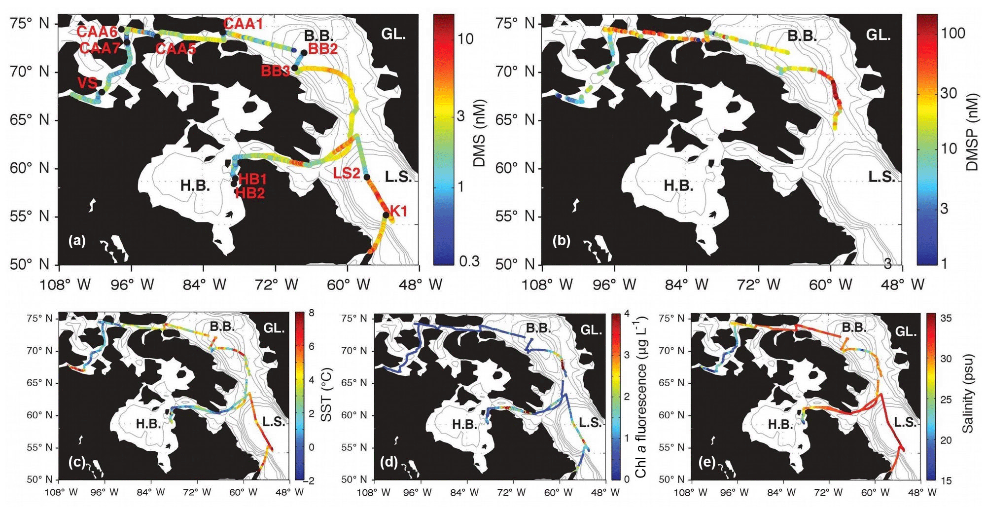
Figure 1 Spatial distribution of DMS, DMSP and hydrographic variables. GL. is Greenland, B.B. is Baffin Bay, L.S is Labrador Sea, H.B. is Hudson Bay, and C.A.A. is Canadian Arctic Archipelago.

Quantifying the spatial and temporal distribution of DMS and DMSP in the Arctic Ocean is particularly important in light of the rapidly changing hydrographic conditions across this region. Rapid Arctic warming over the past several decades has been associated with a significant reduction in summer sea ice extent, resulting in higher mixed layer irradiance levels and a longer phytoplankton growing season (Arrigo et al., 2008). Arrigo et al. (2008) suggested that continued warming and sea ice loss could lead to a 3-fold increase in primary productivity over the coming decades. The effects of these potential changes on DMS(P) concentrations and cycling remain unknown, but it has been suggested that future changes in Arctic Ocean DMS emissions could modulate regional climatic patterns (Levasseur, 2013). Indeed, modelling work has suggested that cooling associated with increased DMS production and emissions in less-ice-covered polar regions may help offset warming associated with loss of sea ice albedo (Gabric et al., 2004; Cameron-Smith et al., 2011). The important climatic and biological roles of reduced sulfur compounds, combined with altered marine conditions under a warming environment, provide the motivation for a deeper understanding of the distribution and cycling of DMS and related compounds in Arctic waters.

In this article, we present a new dataset of DMS and DMSP concentrations in Arctic and subarctic waters adjacent to the Canadian continental shelf. We used a number of recent and emerging methodological approaches to measure these compounds in a continuous ship-board fashion. In particular, we used membrane-inlet mass spectrometry (MIMS) to measure DMS with extremely high spatial resolution (i.e. sub-kilometre scale), as well as the recently developed organic sulfur sequential chemical analysis robot (OSSCAR), for automated analysis of DMS and DMSP. Our goal was to utilize the sampling capacities of the MIMS and OSSCAR systems to make simultaneous measurements of DMS(P) in subarctic Atlantic and Arctic waters, in order to expand the spatial coverage of the existing DMS(P) dataset and identify environmental conditions leading to spatial variability in the concentrations of these compounds.

2 Methods

2.1 Study area

Our field study was carried out on board the CCGS Amundsen during leg 2 of the 2015 GEOTRACES expedition to the Canadian Arctic, from 10 July to 20 August 2015. We sampled along a ∼ 10 000 km transect from Québec City, Québec, to Kugluktuk, Nunavut. Data collection commenced off the coast of Newfoundland and included waters of the Labrador Sea, Baffin Bay and the Canadian Arctic Archipelago (CAA) (Fig. 1).

The cruise transect covered two main distinct geographic domains – the Baffin Bay–Labrador Sea region and the CAA. The majority of the surface water in the CAA is from Pacific-sourced water masses, as a shallow sill near Resolute restricts the westward flow of Atlantic-sourced water (Michel et al., 2006). Flow paths through the CAA are complex. The region is characterized by a network of shallow, narrow straits that are subject to significant regional variability in local mixing and tidal processes and strongly influenced by riverine input, which drives stratification (Carmack and McLaughlin, 2011). In contrast, both Atlantic- and Pacific-sourced waters mix in the Baffin Bay and Labrador Sea regions, and this confluence drives a strong thermohaline front, leading to lower stratification than in the CAA (Carmack and McLaughlin, 2011).

2.2 Underway sampling systems

We utilized two complementary underway sampling systems to measure reduced sulfur compounds: MIMS (Tortell, 2005) and OSSCAR (Asher et al., 2015). Detailed methodological descriptions of these systems have been published elsewhere (Tortell, 2005; Tortell et al., 2011; Asher et al., 2015), and only a brief overview is given here.

2.2.1 OSSCAR

The OSSCAR instrument consists of an automated liquid handling/wet chemistry module that is interfaced to a custom-built purge-and-trap gas chromatograph (GC) equipped with a pulsed flame photometric detector (PFPD) for sulfur analysis. A custom LabVIEW program is used to automate all aspects of the sample handling and data acquisition. During analysis, unfiltered seawater (3–5 mL) from an underway supply (nominal sampling depth ∼ 5 m) is drawn via automated syringe pump into a sparging chamber. DMS is then stripped out of solution (4 min of 50 mL min⁻¹ N₂ flow) onto a 0.125 in. stainless steel trap packed with carbopack at room temperature. Rapid electrical heating of the trap (to ∼ 260 ^∘C), causes DMS desorption onto a capillary column (Restek SS MXT, 15 m, 80 ^∘C, 2 mL min⁻¹ N₂ flow) prior to detection by the PFPD (OI Analytical, model 5380). Light emitted during combustion in the PFPD is converted to a voltage and recorded by a custom built LabVIEW data acquisition interface. Following the completion of DMS analysis, 5 M sodium hydroxide is added to the sparging chamber for 14 min to cleave DMSP in solution to DMS, following the method of Dacey and Blough (Dacey and Blough, 1987). The resulting DMS is sparged out of solution and measured as described above. The sparging chamber is then thoroughly rinsed with Milli-Q water, and the process can be repeated. As we used unfiltered seawater for our analysis, it is important to note that we measured total DMSP (DMSP_t) concentrations, which represent the sum of dissolved and particulate pools.

We measured an in-line standard (20 nM) every four to five samples (at most every 3 h) to ensure that the system was functioning correctly and to correct for potential detector drift. The mean standard error of daily point standards was 0.55 nM, and we consider this to represent the precision of our emerging method (significant efforts are underway to increase this precision). To correct the underway data for instrument drift, point standard measurements were smoothed with a three-point running mean filter, interpolated to the time points of sample measurements and compared to the known standard concentration to provide a drift correction factor for every seawater data point. Six-point calibration curves were performed every 2 days, using DMS standards (ranging from 0 to 18 nM), produced from automated dilutions of a primary DMS stock and Milli-Q water (see Asher et al., 2015). The limit of detection of the system was calculated from the calibration curve using the formula C_LOD= 3 s_y∕x/b, where C_LOD is the concentration limit of detection, s_y∕x is the standard error of the regression and b is the slope of the regression line. With this approach, we derived a mean limit of detection of 1.4 nM. The mean linear calibration curve R² value, taken over all calibration curves, was 0.9887.

The OSSCAR system is designed to automate the collection of seawater for sequential analysis of DMS, dimethylsulfoxide (DMSO) and DMSP in a single sample. During our cruise, however, we experienced problems with the DMSO reductase enzyme used to convert DMSO to DMS for analysis, and we therefore configured the instrument to run only DMS and DMSP at sea, with one cycle requiring roughly 30 min. We experienced general technical difficulties with the instrument during the early phases of the cruise, and no OSSCAR data are thus available for the first half of the transect.

2.2.2 MIMS

We used MIMS to obtain very high-frequency measurements (∼ several data points per minute) of DMS concentrations and other gases in surface seawater. Using this system, seawater from the ship's underway loop was pumped through a flow-through sampling cuvette, attached, via a silicone membrane, to a quadrupole mass spectrometer (Hiden Analytical HPR-40). DMS was measured by detecting ions with a mass to charge ratio of 62 (m∕z 62) every ∼ 30 s. To achieve constant sample temperature prior to contact with the membrane, seawater was passed through a 20 foot coil of stainless steel tubing immersed in water bath held at 4 ^∘C (Tortell et al., 2011). The system pressure (as measured by the Penning Gauge) remained stable during operation (∼ 1.3–1.5 × 10⁻⁶ Torr). The DMS signal was calibrated using liquid standards that were produced by equilibrating 0.2 µm filtered seawater with a constant supply of DMS (m∕z 62) from a calibrated permeation device (VICI Metronics). The primary effluent from the permeation tube (held at 30 ± 0.1 ^∘C in a custom-built oven) was split among several capillary outflows and mixed into a N₂ stream controlled at 50 mL min⁻¹ using a pressure regulator and fixed length and diameter tubing. This system enabled us to achieve a range of DMS ∕ N₂ mixing ratios that were bubbled into standard bottles held in an incubator tank supplied with continuously flowing seawater. Concentrations of DMS in the standard bottles were cross-validated by measuring discrete samples using the OSSCAR system. The limit of reliable detection of the MIMS is ∼ 2 nM (Tortell, 2005).

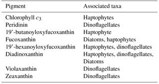
Table 1 HPLC marker pigments and their associated phytoplankton taxa. Adapted from Coupel et al. (2015).

2.3 Post-processing of DMS data

Raw data outputs (voltages) for both OSSCAR and MIMS measurements were processed into final concentrations using MATLAB scripts. For OSSCAR data, raw voltages were captured with a sampling frequency of 5 Hz. Sulfur peaks eluting off the GC column were integrated using a custom MATLAB script, with correction for baseline signal intensities. DMS concentrations were derived from peak areas using the calibration curves as described above.

2.4 Ancillary seawater data

Shipboard salinity, temperature, wind speed and chlorophyll a (chl a) fluorescence measurements were collected using several underway instruments. We used a Seabird Electronics thermosalinograph (SBE 45) for continuous surface temperature and salinity measurements and a Wetlabs Fluorometer (WetStar) to measure chl a fluorescence, as a proxy for phytoplankton biomass. We note that the chl a fluorescence data are subject to significant diel cycles associated with light-dependent fluorescence quenching. All sensors were calibrated prior to and following the summer expedition. Conductivity temperature depth profiles were used to measure vertical profiles of salinity and potential temperature at 17 stations, from which we computed density using the Seawater Toolbox in MATLAB. The MLD was defined as the depth where density exceeded surface values by 0.125 kg m⁻³. Sea ice concentrations were obtained from the AMSR-E satellite product (Cavelieri et al., 2006) with a spatial resolution of 12.5 km. The percent ice cover along the cruise track was derived from a two-dimensional interpolation of the ship's position in time and space against the daily sea ice data.

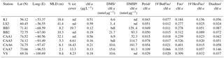
Table 2 Mixed layer depth (MLD), ice cover, HPLC pigment measurements (ratios of selected marker pigments to chl a), DMS (MIMS) and DMSP (OSSCAR) measurements. Perid is peridinin, 19'ButFuc is 19'-butanoyloxyfucoxanthin, Fuc is Fucoxanthin, 19'HexFuc is 19'-hexanoyloxyfucoxanthin, and Diadino is Diadinoxanthin. nd means no data. bdl means below detection limit.

All correlation analyses (Pearson's r) were computed in MATLAB, using the corrcoef function. Sample sizes were as follows: 33 250 data points in the MIMS DMS dataset, 344 in the OSSCAR DMS dataset and 318 in the OSSCAR DMSP dataset.

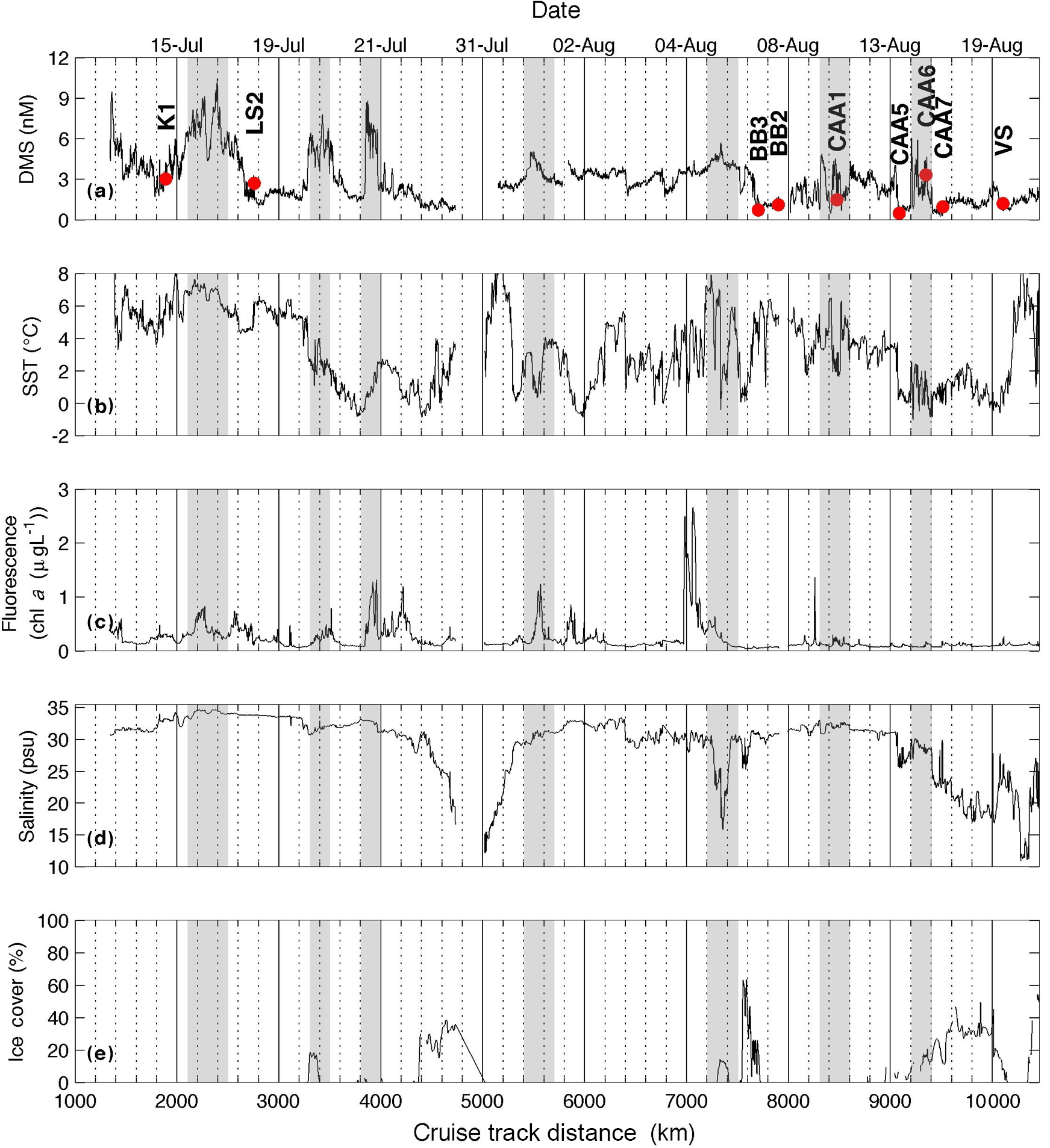
Figure 2 Distribution of DMS and hydrographic variables along our cruise track. Grey shaded areas denote regions of sharp increases in DMS. Labelled red dots indicate sampling stations (see Table 2).

2.5 Phytoplankton biomass and taxonomic composition

In addition to underway data, samples for the quantification of photosynthetic and accessory pigments (Table 1) were collected at a number of discrete oceanographic stations (see Table 2). For each station, duplicate samples (250–500 mL) for chl a analysis were filtered onto pre-combusted 25 mm glass fiber filters (Whatman GF/F) using low vacuum pressure (< 100 mm Hg). Filters were stored at −20 ^∘C and chl a was determined within a few days of sample collection using fluorimetric analysis following the method of Welschmeyer (Welschmeyer, 1994). Duplicate 1–2 L samples were filtered onto pre-combusted 25 mm GF/F for pigment analysis by reverse-phase high-performance liquid chromatography (HPLC). Filters were dried with absorbent paper, flash frozen in liquid nitrogen and stored at −80 ^∘C until analysis following the method of Pinckney et al. (1994). We used several diagnostic pigments as markers for individual phytoplankton groups, as described by Coupel et al. (2015) (see Table 1). Following HPLC pigment processing, data were interpreted with the chemotaxonomy program CHEMTAX V1.95, using the pigment ratio matrix described by Taylor et al. (2013).

Table 3 CHEMTAX-derived phytoplankton assemblage estimates (numbers given are percent of total chl a) for sampled stations. Diat. is diatoms; Dinoflag is Dinoflagellates; Chloro. is Chlorophytes; Prasino is Prasinophyte (types 2 and 3); Crypto. is Cryptophytes; Chryso-Pelago is Chrysophytes/Pelagophytes; c3-flag. is c3-Flagellates; Hapto-7 is Haptophyte type 7. Due to the presence of unidentified phytoplankton taxa, not all assemblage estimates sum to 100 %.

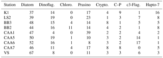
Figure 3 Distribution of DMS and DMSP along the cruise track. Panel (a) shows DMS measurements made by MIMS and OSSCAR. Note that a small fraction (less than 0.5 %) of measurements made by OSSCAR were above 12 nM. Panel (b) shows MIMS data with OSSCAR DMSP measurements superimposed on a different y scale (right-hand side). Labelled red dots indicate DMS concentrations measured at discrete sampling stations (see Table 2).

2.6 DMS sea–air flux

We derived sea–air fluxes of DMS from MIMS measurements of DMS concentrations, as these data had higher resolution and spatial coverage than OSSCAR observations. We computed sea–air flux as

$$\begin{array}{}\text{(1)}& {\displaystyle }{F}_{\mathrm{DMS}}=k_{\mathrm{DMS}}\left({\mathrm{DMS}}_{\mathrm{sw}}\right)(\mathrm{1}-A{)}^{\mathrm{0.4}},\end{array}$$

where DMS_sw is the concentration of DMS in the surface ocean (surface atmospheric DMS is assumed to be zero) and k_DMS is the gas transfer velocity derived from the equations of Nightingale et al. (2000), normalized to the temperature- and salinity-dependent DMS Schmidt number of Saltzman et al. (1993). The term A represents the proportion of sea ice cover, and the scaling exponent of 0.4 accounts for the effects of sea ice on gas exchange and is derived from the laboratory work of Loose et al. (2009). (We note that this scaling does not capture all processes present in sea-ice-dominated regimes, such as turbulence generated by sea ice melt.) Sea-surface salinity and temperature measurements described in Sect. 2.5 were used in the calculations. Wind speed data were obtained from the ship's anemometer (AAVOS data, Environment Canada), corrected to a height of 10 m above the sea surface.

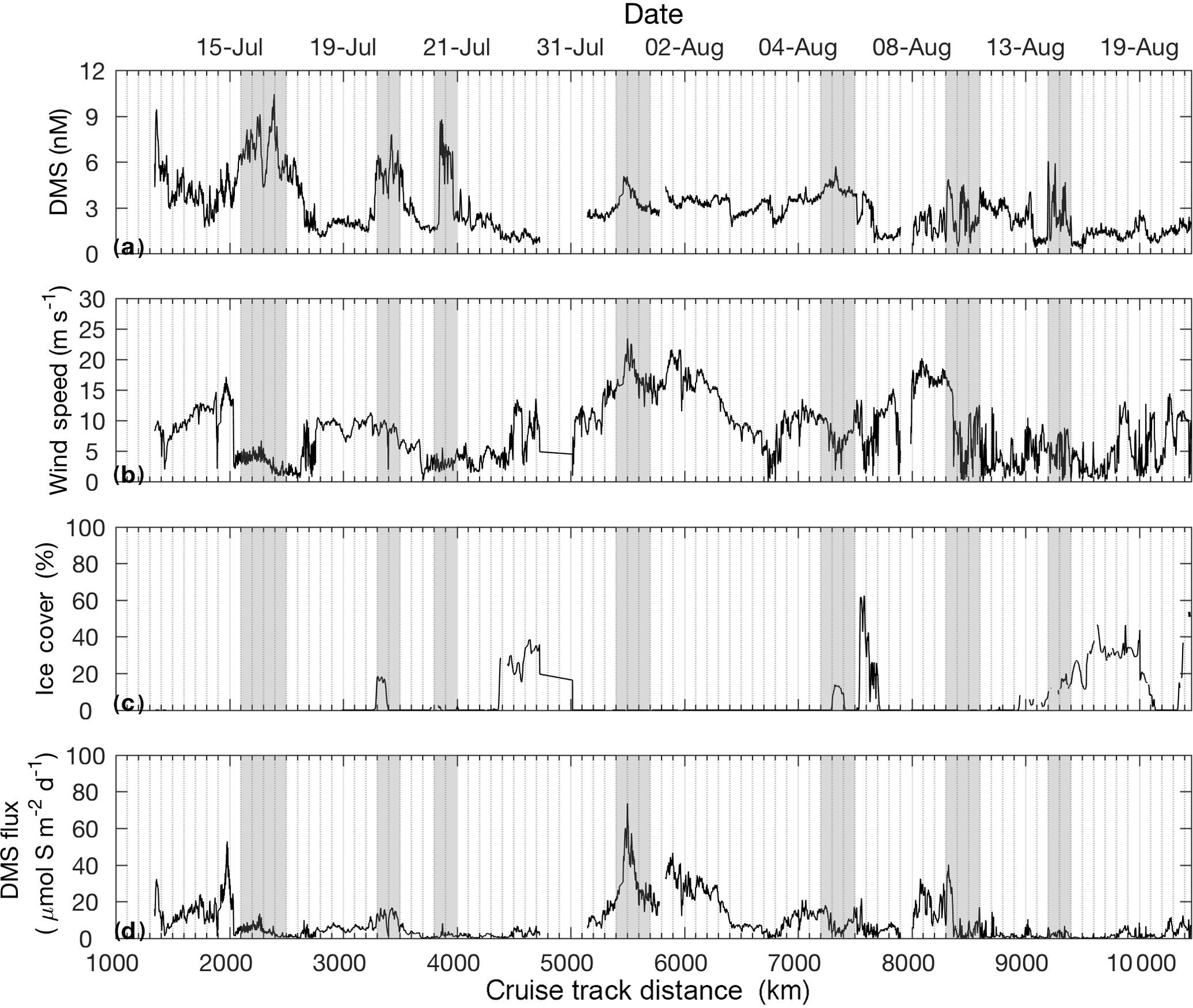
Figure 4 Distribution of DMS, wind speed, sea ice cover and sea–air DMS flux along the cruise track.

3 Results

3.1 Oceanographic setting

Figures 1 and 2 show the distribution of hydrographic properties across our cruise survey region. Over our sampling area, surface water temperatures varied between −1.2 and 10.2 ^∘C, while surface salinity ranged from 10.7 to 34.7 psu (Fig. 1). The warmest and most saline waters were found in the Labrador Sea, with cold fresher waters in Hudson Strait and the CAA. Underway chl a fluorescence varied between 0.04 and 2.96 µg L⁻¹, averaging 0.20 µg L⁻¹. The highest chl a fluorescence was observed in a localized region within Baffin Bay, in the vicinity of a sharp temperature and salinity frontal zone (Fig. 1). MLD ranged from ∼ 5 to 50 m and were deepest in the Labrador Sea and shallowest in the stations of the CAA. Sea ice cover was variable across the survey transect, with ice-free waters in the Labrador Sea and significant ice cover in the northern Hudson Bay and parts of the CAA (Fig. 2).

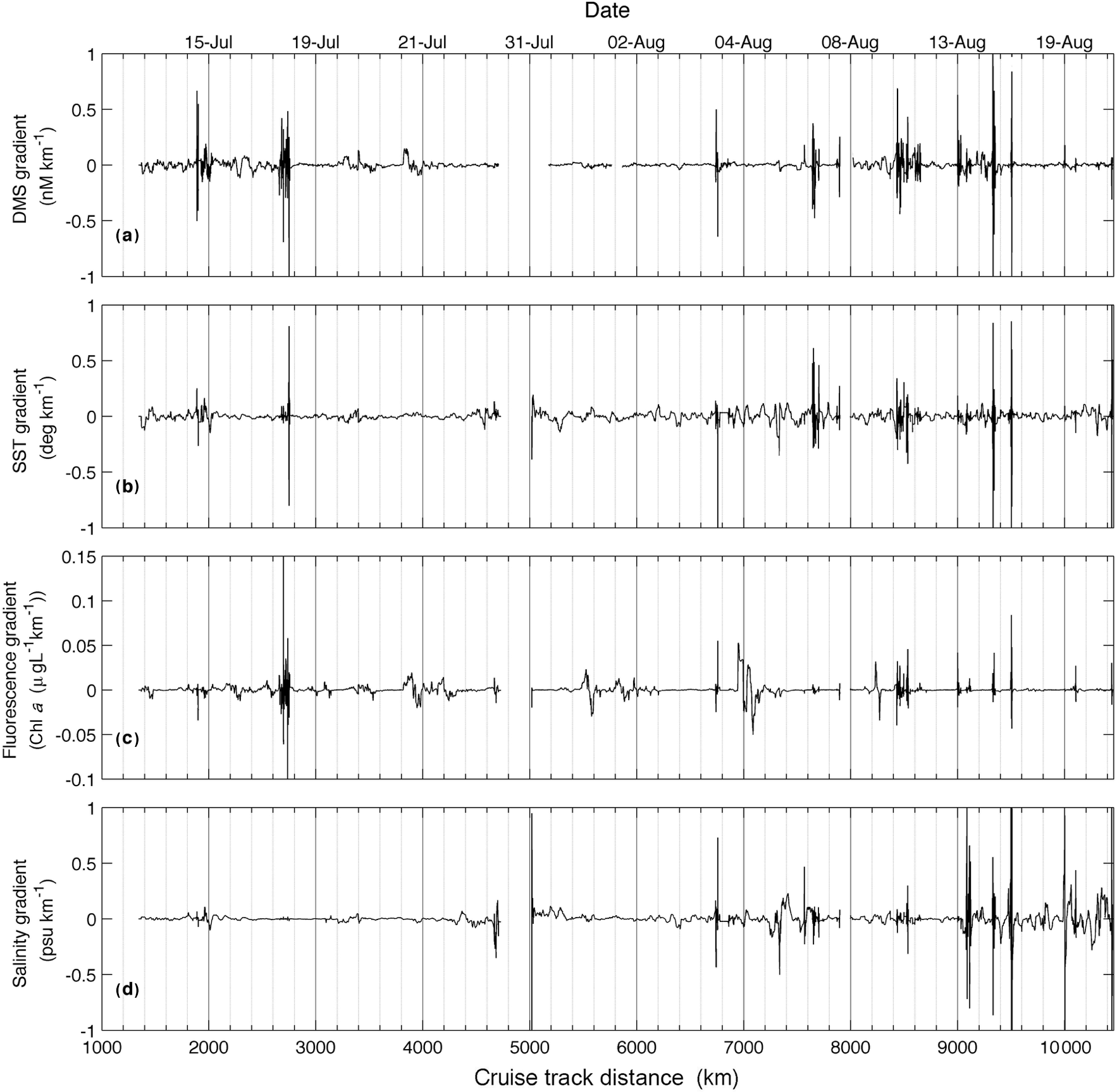
Figure 5 Spatial gradients in DMS (measured with MIMS) and hydrographic variables, calculated from a neighbourhood of 100 data points (∼ 25 km).

3.2 Phytoplankton biomass and taxonomic distributions

Using measurements of accessory photosynthetic pigments, we examined spatial patterns in the taxonomic composition of phytoplankton assemblages (see Table 1 for a description of HPLC marker pigments and their associated phytoplankton taxa). The distribution of pigments across our sampling stations is presented in Table 2, along with measurements of mixed layer depth and ice cover, while CHEMTAX-derived assemblage estimates are shown in Table 3. In order to remove large potential differences in total phytoplankton biomass, we normalized pigment concentrations to total chl a concentrations measured using HPLC (see Methods, Sect. 2.5).

CHEMTAX pigment analysis shows that all stations in the study area were diatom-dominated, although haptophyte, dinoflagellate and prasinophyte markers were detected in varying quantities at all stations (see Table 3). Total HPLC-measured chl a was relatively low throughout the study area, ranging from 0.11 to 0.56 µg L⁻¹.

3.3 Observed DMS(P) concentration ranges

The DMS data shown in Fig. 1 are derived from MIMS measurements, since these have wider geographic coverage and greater spatial resolution than OSSCAR data. DMS concentrations measured with MIMS ranged from 0.2 to 12 nM, averaging 2.7 (±1.5) nM. The highest values were observed in the northern Labrador Sea, Baffin Bay and Hudson Strait, with lower values through much of the Arctic Archipelago.

Figure 3 shows the distribution of DMS, measured by both MIMS and OSSCAR, along the cruise track. DMS concentrations measured with OSSCAR ranged from 0.1 to 18 nM, averaging 3.2 ± 2.4 nM. As described in the discussion, 22 % of our derived DMS concentrations fell below the limit of detection. In general, we observed reasonably good coherence between DMS measurements made by our two analytical systems, with similar absolute values of data and spatial patterns. There were, however, notable offsets in the early August measurements (∼ kilometre 7000 along the cruise track, Fig. 3a), when OSSCAR DMS data were consistently higher than MIMS data. Notwithstanding this offset (for which potential reasons are addressed in the discussion), the coherent spatial patterns in data derived from these independent methods is encouraging, particularly given the rather low precision of our current OSSCAR system.

The spatial distribution of DMSP concentrations (measured with OSSCAR) along the cruise track is also shown in Fig. 3. Concentrations ranged from < 1 to 160 nM, and averaged 30 ± 29 nM. DMSP : chl a ratios measured from HPLC chl a data ranged from 52.31 to 181.4 nmol µg⁻¹. Examination of the data in Fig. 3 reveals that high DMS concentrations were sometimes, but not always, accompanied by high DMSP concentrations. For example, a sharp increase in measured DMSP concentrations (around 7000–7400 km) on the cruise track was accompanied by a sharp increase in DMS measured by both instruments, while low-DMS waters observed around 9400 km along the transect also showed very little DMSP. Over the portion of the transect where measurements of both DMS and DMSP were available, the OSSCAR-measured concentrations of these compounds exhibited a statistically significant positive correlation (r= 0.52, p < 0.001). There were, however, a number of regions where increased DMS concentrations were not accompanied by increases in DMSP (e.g. ∼ 10 000 km).

3.4 Sea–air flux

Figure 4 shows DMS sea–air fluxes as computed from MIMS-measured DMS seawater concentrations, wind speed and sea ice cover. DMS sea–air fluxes ranged from < 1 to 80 µmol S m⁻² day⁻¹, with peak sea–air flux calculated around 5500 km on the cruise track. Sea–air flux is highly dependent on wind speed and sea ice cover, with the result that even high concentrations of seawater DMS yielded low sea–air flux when low wind and/or high sea ice was present (e.g. 2100, 7200, 8300 km). Conversely, very high sea–air fluxes were observed when moderately high DMS concentrations coincided with high wind speeds and ice-free waters (e.g. 5400 km).

3.5 Comparison of gradients in DMS data with hydrographic features

The high sampling frequency of MIMS measurements allows the comparison of DMS observations with other underway environmental variables and enables the quantification of small-scale DMS concentration gradients in near real time. Figure 2 shows a cruise track record of MIMS-measured DMS concentrations in relation to salinity, temperature, chl a fluorescence and ice cover. Several sharp increases in DMS at around 2100, 3300 and 3800 km along the cruise track were accompanied by strong gradients in temperature and, to a lesser extent, salinity (Fig. 2). These regions correspond to areas in the Labrador Sea and Baffin Bay. An increase in DMS concentrations in Baffin Bay around 7200 km in the cruise track (Fig. 2a) was associated with a simultaneous drop in sea-surface temperature and salinity, in close proximity to a sharp increase in chl a fluorescence along the cruise track (see Figs. 1 and 2c). As shown in Fig. 3b, this localized region exhibited the highest concentrations of DMSP along the transect. Interestingly, this area was also characterized by strong gradients in sea ice concentrations, and the low salinity waters are indicative of localized ice melt. Figures 1d and 2d also show the large-scale salinity gradients in the Hudson Bay and the Canadian Arctic Archipelago, highlighting the freshwater influx in these near-shore areas. In contrast to our observations in Baffin Bay, DMS concentrations showed relatively little variability across these salinity gradients.

In order to more closely examine small-scale variability in DMS and other surface water variables, we calculated spatial gradients in the data to examine the coherence of frontal features in DMS, salinity, temperature and chl a fluorescence. For this analysis, we computed gradients in each oceanographic variable within a neighbourhood of 100 points surrounding each point. Gradients (G) for each variable (DMS, sea-surface temperature, chl a and salinity) were calculated at each point x as follows:

$$\begin{array}{}\text{(2)}& G_x={\displaystyle \frac{V_{x+\mathrm{50}}-V_{x-\mathrm{50}}}{D_{x+\mathrm{50}}-D_{x-\mathrm{50}}}}.\end{array}$$

Here, G is gradient (in units of change per km), V is the value of the variable at a point, x, and D is the cruise track distance at x. A neighbourhood of 100 points, corresponding to a distance of ∼ 25 km, was subjectively chosen because it best captured the observed variability in the data, representing an intermediate value between a localized neighbourhood (e.g. 10 points), which would only consider changes close to the point, and a large neighbourhood (e.g. 1000 points), which would smooth the features. The results of this analysis (Fig. 5) qualitatively demonstrate a coherence of DMS gradients with salinity, chlorophyll and sea-surface temperature.

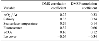
Table 4 Pearson correlation coefficients relating DMS measurements made by MIMS and DMSP measurements made by OSSCAR to other oceanographic variables. Only correlations significant at the p < 0.05 level are shown. ΔO₂ ∕ Ar ratios were obtained using MIMS.

3.6 Correlation with ancillary oceanographic variables

We computed Pearson correlation coefficients of DMS and DMSP with underway measurements of salinity, sea-surface temperature, chl a fluorescence and sea ice cover. We also examined the potential relationships between DMS concentrations and MIMS-derived pCO₂ and ΔO₂ ∕ Ar (Philippe Tortell, personal communication, 2017). The results can be seen in Table 4. Only correlations significant at the 0.05 level are included. Only weak correlations are seen between MIMS-measured DMS data and ancillary variables, and OSSCAR DMS data did not exhibit any significant correlations with any ancillary variables, including measured of phytoplankton taxonomic distributions. A significant positive correlation (r= 0.66, p < 0.001) was found between DMSP and underway chl a fluorescence. Over the whole transect, we observed a weak negative correlation between DMS(P) and sea ice cover (r= −0.26 for DMS and r= −0.34 for DMSP; p < 0.001 in both cases). A weak positive correlation was found between DMSP ∕ chl a and ice cover (r= 0.52, p < 0.04), suggesting potential roles for sea ice microalgae in DMSP production at the sampled stations. It is interesting to note that elevated chl a fluorescence and DMSP concentrations often occurred in areas of intermediate ice cover (3300, 7300 and 9200 km along the cruise track), potentially reflecting the influence of ice-edge blooms or under-ice phytoplankton assemblages. Potential mechanisms for these features are addressed in the discussion.

4 Discussion

Our results provide a new dataset of reduced sulfur compounds in an under-sampled region of the Arctic Ocean, enabling an examination of DMS(P) variability in relation to various oceanographic properties on a range of spatial scales. Below, we focus our discussion on the observed relationship between gradients in DMS and other oceanographic variables, and discuss the comparability of the two DMS measurement methods utilized. We compare our results to previously published measurements in the Arctic, situating our results in the context of the changing hydrography and phytoplankton ecology of the Arctic Ocean.

4.1 Comparability of MIMS and OSSCAR measurements

The OSSCAR and MIMS instruments have previously shown good agreement in measured DMS concentrations in the subarctic Pacific Ocean (Asher et al., 2015). Similarly, we observed relatively good coherence between the two methods (Fig. 3) over much of our cruise track. The largest exception to this occurred around kilometre 7000, when DMS measurements measured by OSSCAR were significantly higher than those measured by MIMS. This region was characterized by very high DMSP measurements (often 1 order of magnitude higher than the DMS measurements). If small amounts of DMS remained in the OSSCAR system after DMSP analysis, sample carryover could contribute to higher measured concentrations in the subsequent DMS analysis. In order to minimize this potential artefact, the system was thoroughly rinsed with Milli-Q water after every run. The effectiveness of this rinse was tested by subsequently purging DMSP standards without NaOH, and no carryover was observed. It is possible, however, that this approach was not entirely efficient. Another potential cause of the higher OSSCAR DMS measurements may be due to cell breakage during the sparging process in OSSCAR. In this scenario, there is the potential for release of intracellular DMSP and DMSP lyase into solution, which would lead to artificially high measured DMS concentrations. It is not possible for us to quantify the magnitude of such a potential artefact, but we note that its magnitude would likely depend on the taxonomic composition of phytoplankton assemblages. Wolfe et al. (2002) showed that sample sparging led to an increase in DMS production by both the haptophyte Emiliana huxleii and the dinoflagellate Alexandrium. Unfortunately, due to limited coverage of discrete sampling, we do not have any estimates of phytoplankton community composition in the region where MIMS and OSSCAR showed the greatest discrepancies. Notwithstanding these potential caveats, we suggest that the two methods show strong promise to provide complementary information on DMS(P) (and DMSO) concentrations in surface ocean waters.

One challenge going forward is to increase the reproducibility and sensitivity of OSSCAR measurements, and this is an area of active work in our group. The version of our system used in 2015 had a detection limit of roughly 1.4 nM and was thus far less sensitive than many conventional GC methods, which can achieve sub-nanomolar detection limits. Our detection limit was of only minor consequence for DMSP measurements, given that 72 % of measured DMSP concentrations were higher than 10 nM, and less than 3 % fell below 1.4 nM. The relatively low sensitivity was somewhat more problematic for DMS, with approximately 22 % of our OSSCAR-measured DMS values below 1.4 nM. Nonetheless, as discussed below, we believe that the OSSCAR data, in combination with our MIMS data, provide useful information on the spatial distribution of both DMSP and DMS in Arctic waters.

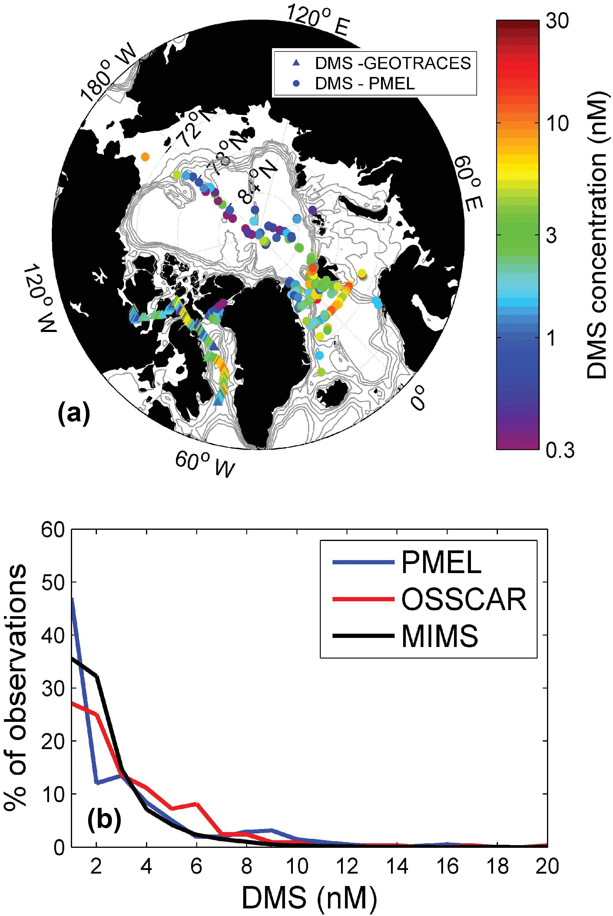
Figure 6 Comparison of OSSCAR- and MIMS-measured DMS from this study with existing summertime data in the PMEL database. Panel (a) shows the geographic distribution of DMS measurements in the PMEL database and those obtained by this study (using OSSCAR), while panel (b) shows a histogram of DMS concentrations in three datasets – the MIMS dataset (33 250 data points), the OSSCAR dataset (344 points) and the PMEL dataset (415 points).

4.2 Towards a regional Arctic database of DMS(P) concentrations

Figure 6 shows a comparison between our Arctic DMS measurements (made by OSSCAR) and other summertime Arctic DMS data in the PMEL database. For this comparison, only PMEL measurements made above the Arctic circle (66.56^∘ N) in June–August are included, resulting in a total of 415 data points. As shown in Fig. 6, the majority of available summertime PMEL DMS(P) measurements are found in the Atlantic region of the Arctic and in the Bering Sea, with limited data in the Canadian Archipelago (for an overview of Arctic DMS(P) studies performed to date, see Levasseur, 2013). For the sake of visual clarity, the presentation of data in Fig. 6a is based on DMS measurements made by OSSCAR, whereas both sets of data were included in the frequency distribution analysis (Fig. 6b). The results presented in Fig. 6 suggest that our measurements are representative of the broader Arctic context, with generally similar data frequency distributions (Fig. 6b) for all three DMS datasets (MIMS, OSSCAR and PMEL). From the map, we see that the spatial footprint of our measurements complement the existing summer data, helping to expand the spatial coverage of DMS observations in the Arctic Ocean.

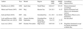
In addition to complementing the existing PMEL DMS database, our new observations also build on a number of other reduced sulfur measurements in the Canadian sector of the Arctic Ocean. Observations of DMS and DMSP derived from several past Arctic and subarctic Atlantic surveys are summarized in Table 5. This table focuses mainly on DMS and DMSP measurements made in the Canadian sector and Greenland waters, serving to provide context for our measurements performed in similar environments. The data presented in Table 5 are obtained from different times of year and from phytoplankton assemblages of varying taxonomic composition, allowing us to examine DMS and DMSP concentrations in surface waters under a range of environmental and ecological conditions. For example, Bouillon et al. (2002) observed low DMS concentrations (< 1 nM) during a large spring diatom bloom (∼ 15 µg L⁻¹chl a) in the North Water region. In contrast, higher DMS concentrations have been reported later in the season when total phytoplankton biomass is lower, and taxonomic composition has shifted away from diatom dominance. Working in the same geographic region as Bouillon, Motard-Côté et al. (2012) reported higher late summer (September) DMS levels (maximum = 4.8 nM), which were accompanied by moderate chl a concentrations (0.2–1 µg L⁻¹), while Luce et al. (2011) reported very low DMS (< 1 nM) associated with moderate chl a concentrations (0.2–2 µg L⁻¹) in a flagellate-dominated community in late fall (October–November), with DMS decreasing towards the later months. A similar pattern was observed in the northwest subarctic Atlantic by Lizotte et al. (2012), who associated elevated reduced sulfur (DMSP) production with flagellate and prymnesiophyte communities in midsummer and fall, in contrast to early-season diatom blooms with little associated DMSP and DMS. This seasonal decrease in DMS levels may be potentially attributable to light-limited primary productivity and diminishing capacity for light-induced oxidative stress, which has been shown to increase DMS(P) production (Sunda et al., 2002).

To date, the highest recorded Arctic water column measurements of DMS (25 nM) and DMSP (160 nM) have been observed during midsummer blooms of the haptophyte Phaeocystis at the ice edge (see Matrai and Vernet, 1997; Galí and Simó, 2010). Our mid-season (July–August) study of similar areas shows moderately high DMS (up to 18 nM) accompanied by relatively low chl a (0.11–1.06 µg L⁻¹) in a mixed community where flagellates and prasinophytes are present.

Together, the available data (Table 5 and our measurements) are consistent with a seasonal cycle in Arctic and subarctic reduced sulfur distributions. Early-season diatom-dominated blooms exhibit high biomass and primary productivity but low DMS(P) accumulation, while midsummer phytoplankton assemblages dominated by haptophytes and dinoflagellates display lower phytoplankton biomass but higher reduced sulfur accumulation. This pattern is similar to the summertime “DMS paradox” reported in a number of temperate and subtropical waters (Simo and Pedrós-Alió, 1999). In the fall, both Arctic primary productivity and DMS(P) production decrease with the onset of lower temperatures and increased ice cover. Our data are consistent with this general scenario, representing a mixed-species assemblage with moderate biomass and DMS(P) accumulation.

Table 5 Compilation of published Arctic and subarctic Atlantic DMS(P) data from the summer and fall months, focusing on observations from the Western Hemisphere.

4.3 Gradients in DMS and hydrographic frontal structures

The high resolution afforded by the MIMS dataset allows for the observation of fine-scale variability in DMS concentrations at the sub-kilometre scale. Previous studies (Tortell, 2005; Tortell et al., 2011) have quantified fine-scale variability in DMS concentrations, demonstrating de-correlation length scales on the order of tens of kilometres, and often shorter than that of other oceanographic variables such as temperature and salinity. These length scales provide information on the spatial scale of processes driving the majority of variability in DMS concentrations. Figures 2 and 5 clearly demonstrate that gradients in DMS and chl a fluorescence often co-occur with strong gradients in temperature and salinity. This suggests a potential role for hydrographic fronts in driving changes in DMS concentrations. Several potential mechanisms may explain this phenomenon. For example, the frontal mixing of distinct water masses, driven by currents, wind or melting ice, may introduce nutrients into a low-nutrient water column, stimulating localized primary productivity (Tremblay et al., 2011) and potentially increasing DMS(P) production. Note that this localized increase in productivity and potential DMS(P) production would operate independently of the overall seasonal progression towards increased DMS(P) production during the latter summer growth season. Mixing of water masses may also potentially expose water column phytoplankton to light shock or osmotic stress by mixing them upwards in the water column or introducing an abrupt salinity gradient. Both of these factors could contribute to elevated DMSP production, given its hypothesized role as an intracellular osmolyte and antioxidant (Stefels et al., 2007). Although our data do not allow mechanistic interpretation for the underlying causes of DMS variability in surface waters, the high resolution afforded by MIMS measurements enables real-time observations of DMS gradients, which may be useful in the design of future process studies examining the driving forces for elevated DMS accumulation.

4.4 Influence of phytoplankton assemblage composition and mixed layer depth

Previous work has addressed the role of phytoplankton taxonomic composition and irradiance levels (Stefels et al., 2007) in driving the cycling of DMS(P) in marine waters. Here we discuss the potential influence of these factors across our survey region. The majority of the sampled stations were characterized by very shallow MLDs (Table 2) resulting from strong salinity-based stratification of surface waters. Light stress associated with shallow MLD may contribute to elevated DMSP : chl a ratios, and previous studies (Vallina and Simó, 2007) have shown high correlation between solar irradiance and surface DMS concentrations. In our dataset, however, there was no overall correlation between MLD and DMSP : chl ratios. We did, however, observe elevated DMSP concentrations at two stations (BB3 and CAA6) with shallow MLDs.

The elevated DMSP : chl a ratios measured in our study may also reflect the presence of high-DMSP-producing taxa, a phenomenon previously reported by other groups (Matrai and Vernet, 1997; Galí and Simó, 2010; Lizotte et al., 2012). When comparing our DMSP: chl a ratios to other measurements, it is important to note that we measured DMSP_t, while many other groups present DMSP_p, without taking into account the dissolved fraction (DMSP_d). As the dissolved DMSP pool typically makes up a small (though highly variable) portion of the total water column DMSP pool, the use of DMSP does not likely have a large effect on derived DMSP : chl a ratios (Kiene et al., 2000; Kiene and Slezak, 2006). Despite the potential caveats raised above, the DMSP_t : chl a ratios we measured across our sampling stations (52–182 nmol µg⁻¹) were broadly similar to DMSP_p : chl a values found by Motard-Côté et al. (2011) (15–229 nmol µg⁻¹) in the same region in September. In contrast, our measured DMSP_t : chl a ratios are significantly higher than those measured by Luce et al. (2007) (maximum of 39 nmol µg⁻¹) and Matrai and Vernet (1997) (maximum 17 nmol µg⁻¹) at diatom-dominated stations in the Barents Sea. The higher DMSP : chl ratios we measured may be attributable to the presence of mixed (rather than diatom-dominated) assemblages present in the study area at the time of sampling. We cannot, however, draw any firm conclusions on the role of taxonomy in controlling DMSP : chl a, as we were unable to detect any significant correlations between DMSP : chl a and HPLC pigment markers for different phytoplankton groups.

To conclude, our observations do not permit us to establish a firm link between MLD, phytoplankton taxonomy and DMS(P) concentrations. Other factors, including bacterial activity and zooplankton grazing are potential contributing factors, but we lack the data needed to examine the importance of these processes.

4.5 The interaction of DMS(P) and sea ice

The presence of sea ice exerts a strong control on polar phytoplankton by controlling irradiance levels in the water column (Levasseur, 2013), and influencing vertical mixing, stratification and nutrient accumulation. It is thus expected that the presence of sea ice may affect DMS(P) cycling. In a 2010 study, Galí and Simó (2010) found that Arctic sea ice melt drove stratification of nutrient rich surface water, triggering a sharp increase in primary productivity, with associated elevated DMS and DMSP levels. These authors also showed that experimental exposure of phytoplankton to high light conditions (mimicking those that would follow the breakup of sea ice) led to near-total release of intracellular DMSP, providing one possible explanation for elevated DMSP levels in the water column. A number of studies also show that the ice, itself, can be a potentially significant reservoir of reduced sulfur, associated with bottom ice-algae (Levasseur et al., 1994).

The weak negative correlation we observed between sea ice cover and DMS(P) concentration is consistent with the idea that sea ice cover limits insolation, thereby reducing primary productivity and DMS(P) production. In general, the drivers of DMSP and DMS production differ – though DMSP production has been shown to be directly influenced by sea ice melt in under-ice blooms (Galindo et al., 2014), the production of DMS from DMSP is largely dependent on the metabolism of in situ bacterial assemblages (Evans et al., 2007) and may therefore be uncoupled from the influence of ice on phytoplankton activity. It is interesting to note, however, that several sharp increases in DMS (observed with MIMS) occurred simultaneously with the occurrence of small amounts of sea ice (< 20 % total cover) (Fig. 2; 3400 and 7200 km on the cruise track). Limited station data also indicate high DMSP : chl a ratios in areas with a comparatively high sea ice cover, at stations BB3 and CAA6 (Table 2). At the time of our sampling, both of these stations were characterized by very low phytoplankton biomass (0.11 and 0.20 µg L⁻¹ chl a, respectively) and had particularly high DMSP : chl a ratios (129 and 182 nmol µg⁻¹, respectively). This suggests a potential role for ice-edge effects, either through the melt-induced stimulation of reduced sulfur production in DMSP rich phytoplankton taxa or through the release of ice-associated DMSP into the water column. Figure 2d and e show decreased salinity in partially ice-covered areas (e.g. around 4400, 7300 and 9200 km), suggesting some meltwater stratification effects. Previous groups have also reported elevated DMS and DMSP concentrations in partially ice-covered water and ice-edge regions in the Arctic Ocean (Leck and Persson, 1997; Matrai and Vernet, 1997; Galí and Simó, 2010).

5 Conclusion

We present a high-spatial-resolution dataset of reduced sulfur measurements through the Canadian sector of the Arctic Ocean and subarctic Atlantic. We demonstrate the utility of high-resolution DMS measurements for comparison with other oceanographic variables and show the coherence of DMS gradients with fine-scale surface hydrographic structure, suggesting elevated DMS production in some oceanographic frontal zones. We also observed elevated DMS(P) values in partially ice-covered regions, suggesting that ice-edge effects may stimulate DMS(P) production. Our data serve to significantly expand the existing spatial coverage of reduced sulfur measurements in the Arctic, providing a baseline for future studies in this rapidly changing marine environment. Future warming of surface waters and sea ice melt could lead to increased concentrations and sea–air fluxes of DMS, though significantly more observations will be needed to substantiate this.