Canopy area of large trees explains aboveground biomass variations across neotropical forest landscapes

Large tropical trees store significant amounts of carbon in woody components and their distribution plays an important role in forest carbon stocks and dynamics. Here, we explore the properties of a new lidar-derived index, the large tree canopy area (LCA) defined as the area occupied by canopy above a reference height. We hypothesize that this simple measure of forest structure representing the crown area of large canopy trees could consistently explain the landscape variations in forest volume and aboveground biomass (AGB) across a range of climate and edaphic conditions. To test this hypothesis, we assembled a unique dataset of high-resolution airborne light detection and ranging (lidar) and ground inventory data in nine undisturbed old-growth Neotropical forests, of which four had plots large enough (1 ha) to calibrate our model. We found that the LCA for trees greater than 27 m (∼ 25–30 m) in height and at least 100 m² crown size in a unit area (1 ha), explains more than 75 % of total forest volume variations, irrespective of the forest biogeographic conditions. When weighted by average wood density of the stand, LCA can be used as an unbiased estimator of AGB across sites (R² = 0.78, RMSE = 46.02 Mg ha⁻¹, bias = −0.63 Mg ha⁻¹). Unlike other lidar-derived metrics with complex nonlinear relations to biomass, the relationship between LCA and AGB is linear and remains unique across forest types. A comparison with tree inventories across the study sites indicates that LCA correlates best with the crown area (or basal area) of trees with diameter greater than 50 cm. The spatial invariance of the LCA–AGB relationship across the Neotropics suggests a remarkable regularity of forest structure across the landscape and a new technique for systematic monitoring of large trees for their contribution to AGB and changes associated with selective logging, tree mortality and other types of tropical forest disturbance and dynamics.

1 Introduction

In humid tropical forests, tree canopies contribute disproportionately to the exchange of water and carbon with the atmosphere through photosynthesis (Goldstein et al., 1998; Santiago et al., 2004). From a physical standpoint, canopies are rough interfaces formed by crowns of emergent and large trees, regularly disturbed by wind thrusts and gap dynamics. This structurally complex boundary layer is challenging for scaling of biogeochemical fluxes and modeling of vegetation dynamics (Baldocchi et al., 2003). Large canopy trees are among the first to be impacted by storms or heavy precipitation (Espírito-Santo et al., 2010), drought stress (Nepstad et al., 2007; Saatchi et al., 2013; Phillips et al., 2009) and fragmentation (Laurance et al., 2000), potentially leading to tree death and formation of large canopy gaps (Denslow, 1980; Espírito-Santo et al., 2014). Several studies suggest that forest canopies can show fractal properties that tend to evolve from a non-equilibrium state towards a self-organized critical state, involving gap formation and recovery (Pascual and Guichard, 2005; Solé and Manrubia, 1995), with crowns preferentially growing towards more sunlit parts of the canopy (Strigul et al., 2008).

Over the past decade, stand-level canopy metrics have been increasingly derived using small footprint airborne lidar systems (ALS), a widely used remote sensing technique to study the structure of forests (Kellner and Asner, 2009; Lefsky et al., 2002). Lidar-derived mean top canopy height (MCH) is a good predictor of tropical forest aboveground carbon content and its spatial variability (Jubanski et al., 2013), but it does not provide information on the presence of large trees that are important when monitoring changes in forest biomass from logging and other small-scale disturbance (Bastin et al., 2015). Moreover, different forests with the same MCH may differ in their stem density, notably of large trees, and in stand mean wood density, two aspects that are important in constructing a robust model to infer aboveground biomass (AGB) from lidar data (Asner et al., 2012; Mascaro et al., 2011). Ground observations suggest that stem density, basal area, height and crown size of large tropical trees may all be good indicators of forest AGB (Clark and Clark, 1996; Goodman et al., 2014). This implies that including information on crown area of individual large trees should improve carbon stock assessments, as confirmed in temperate and boreal regions (e.g., Packalen et al., 2015; Popescu et al., 2003; Vauhkonen et al., 2011, 2014). In tropical forests, identifying and delineating crowns of large trees is a difficult and time-consuming process due to the layered structure of the forest canopy and overlapping crowns (Zhou et al., 2010, but see Ferraz et al., 2016).

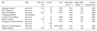
Table 1 Information on forest inventory plots. The ^* symbol indicates that a site has been used for the calibration of the LCA model. Sources: Antimary and Cotriguaçu: (d'Oliveira et al., 2012; Fearnside, 1997), BCI: Center for Tropical Forest Science (CTFS; Condit, 1998; Hubbell et al., 1999, 2005), Chocó: (http://bioredd.org, last access: 13 April 2016), La Selva: Carbono project (Clark and Clark, 2000), Manaus and Tapajós: Fernando Espírito-Santo (unpublished data), Nouragues: (Réjou-Méchain et al., 2015), Paracou: (Gourlet-Fleury et al., 2004; Vincent et al., 2012). Rainfall data from WorldClim (Hijmans et al., 2005). AGB: aboveground biomass, WD: wood density.

Here, we explore how the fractional area occupied by crowns of large trees in a forest stand can be used as a reliable indicator of forest biomass across a wide range of forest structure, climate and edaphic geographic variations. We define large tree canopy area (LCA) as a metric capturing the cluster of crowns of large trees within a forest patch using height and crown area measured by high-resolution airborne lidar measurements. Precisely, LCA is the number of pixels in the canopy height model above a reference height, and excluding the pixel clusters smaller than a reference area. Since this metric quantifies the proportional presence of large trees, it can be used to estimate AGB and monitor changes associated with the disturbance of large trees from mortality events and selective logging. We first explore the properties of LCA across a range of landscapes in the Neotropics. Next, we hypothesize that LCA is a good predictive metric for the spatial variations in AGB over a wide range of old-growth forests.

To this end, we assembled a collection of airborne lidar measurements and ground inventory data at nine sites in old-growth Neotropical forests. The lidar data provide variations in canopy height and distribution of large trees that allow us to address the following questions: (1) is there a single definition of LCA at the landscape scale across different sites? (2) Does the LCA metric capture variations in AGB?

2 Materials and Methods

2.1 Study sites

We studied the canopy structure at nine old-growth lowland Neotropical forest sites that span a broad range of climatic and edaphic conditions (Fig. S1 in the Supplement, Table 1). All sites are located in low elevation areas (less than 500 m above sea level) but have small-scale surface topography that may influence the distribution of crown formations and gaps. These forests are for the most part undisturbed terra firme forests. Tapajós, Antimary and Cotriguaçu get the least rainfall, with approximately 2000 mm yr⁻¹, while La Selva and Chocó both receive more than 4000 mm yr⁻¹ (Table 1).

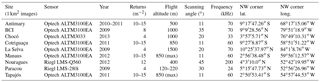
Table 2 Information on lidar data and locations of the nine research sites.

Permanent forest-inventory plots were available for all sites except Cotriguaçu (Table 1). Sites where tree-level inventory data were available were used to estimate the stand-level AGB, hereafter referred to as AGB_inv: BCI (50 plots of 1 ha each), Chocó (42 plots of 0.25 ha each), La Selva (11 plots of 1 ha each), Manaus (10 plots of 0.25 ha each), Nouragues (7 plots of 1 ha each) and Tapajós (10 plots of 0.25 ha each). In these plots, all trees with a diameter at breast height (DBH) ≥ 10 cm have been mapped, measured and the species identified. Trees with irregularities or buttresses were measured higher on the bole. Total tree height measurements were available for a subset of these trees. The method for calculating AGB_inv from forest inventories is reported in Sect. S1 of the Supplement. Four sites (BCI, La Selva, Nouragues and Paracou) with 1 ha inventory plots, were used as “calibration sites” to compare the LCA metric and AGB. Sites with smaller plots were not used as calibration of LCA because of the probability of crowns of large trees extending outside the plot boundary and the introduction of uncertainty in estimating LCA from edge effects (Meyer et al., 2013; Packalen et al., 2015). For this reason, all plots smaller than 1 ha were excluded from the LCA analysis but were used in estimating average wood density (WD) for each site, which does not depend on plot size. Stand-averaged WD was calculated based on the WD of all trees present in a site, determined using the commonly used Global Wood Density Database, and is reported in Table 1 (Chave et al., 2009; Zanne et al., 2009). For Cotriguaçu, we used stand-averaged WD given by Fearnside (1997) for a region covering the site. Additional plot-level data (AGB_inv and mean WD) were provided for Antimary (50 plots of 0.25 ha each), Nouragues (27 plots of 1 ha each) and Paracou (85 plots of 1 ha each).

2.2 Lidar data

Lidar sensors scan the vegetation vertical structure and return a three-dimensional point cloud derived from the time it took each pulse to return to the instrument. The lidar datasets acquired over the study sites come from discrete return lidar instruments and were gridded horizontally at a 1 m resolution using the echoes classified as either vegetation or ground. They yield three products: a digital surface model (DSM) corresponding to the top canopy elevation, digital terrain model (DTM) corresponding to the ground elevation and canopy height model (CHM), which is the height difference between the DSM and the DTM. DTMs were interpolated from a Delaunay triangulation or comparable interpolation methods, after outliers were removed. DSMs were created using the highest return within a cell. Lidar data over Paracou were acquired in last return mode, causing a bias of 50 cm on the CHM (Vincent et al., 2012). This bias is not addressed in this study because our height increment for the determination of optimal height thresholding is larger (1 m; see Sect. 4.3). Data were acquired between 2009 and 2013, using relatively similar sensors and acquisition configurations (Table 2). The potential differences between the lidar datasets and their impact on the results are addressed in the Discussion.

For each site, we selected a 1 km × 1 km (100 ha) area of old-growth forest, oriented north–south, without any human disturbance to the extent possible. Topography derived from lidar data within the selected 1 km² subset images provides information on landscape variations that may impact the forest structure. Data visualization was done using ENVI version 4.8 (Exelis; ENVI/IDL, 2010).

2.3 Computing large canopy area (LCA)

At each study site, we extracted the area of canopy that relates to total area of the canopy height model above a standard height (h) threshold, or LCA(h), and explored how this metric scales along two axes. First, we varied the threshold height h with increments of 1 m, between 5 and 50 m, in 100 m by 100 m subareas (100 subareas for each site). Second, to denoise the data, we excluded the clusters with less than a set number of 1 m² pixels (50, 100, 150 or 200). We then prioritized the crown area of large trees, and filtered out pixels that could be related to outliers or to single branches. This method thus quantifies the area of large crowns covering a plot or larger landscape unit area, as a percentage of covered area.

Figure 1 Segmentation of the 1 km × 1 km images in each site using five canopy height thresholds. A minimum of 100 contiguous pixels was used as a segmentation threshold in all cases.

LCA maps were produced at 1 ha resolution. Pixel clustering was based on the similarity of the four nearest neighbors (similar results were obtained with an eight neighbor model, results not shown here). Figure S2 summarizes the steps taken to go from the lidar canopy height model to the final LCA map. Processing was conducted using the IDL software (interface description language, Exelis; ENVI/IDL, 2010).

We determined the optimal minimum canopy height threshold calculating the coefficient of correlation between AGB_inv and LCA at the four calibration sites. This step allowed us to examine if optimal height thresholds differed from one site to the other. The goal was to find a single optimal height threshold and crown size that could be applied for LCA retrieval across closed-canopy Neotropical forests. We also estimated AGB from lidar data locally (AGB_Local) using a commonly used model fit relating MCH to AGB_inv in each site, to further examine the variations of LCA and AGB in all nine sites (see Sect. S2, Table S1 in the Supplement).

2.4 Relating LCA to biomass

We tested different models to infer AGB_inv from LCA, henceforth called AGB_LCA, at the four calibration sites, and explored if adding more parameters (such as mean WD of a site, mean WD of large trees (DBH ≥ 50 cm), mean canopy height or top percentiles of canopy height) improved the predicting power of the model. We evaluated our results by applying a jackknife validation to our regression models, based on 1000 iterations of bootstrapping. The coefficients of correlation (R²), root mean square error (RMSE) and bias (mean difference between the expected values of AGB and the observed values of AGB) are reported for the models providing the best results. The analysis was performed using the R statistical software (R Core Team, 2014).

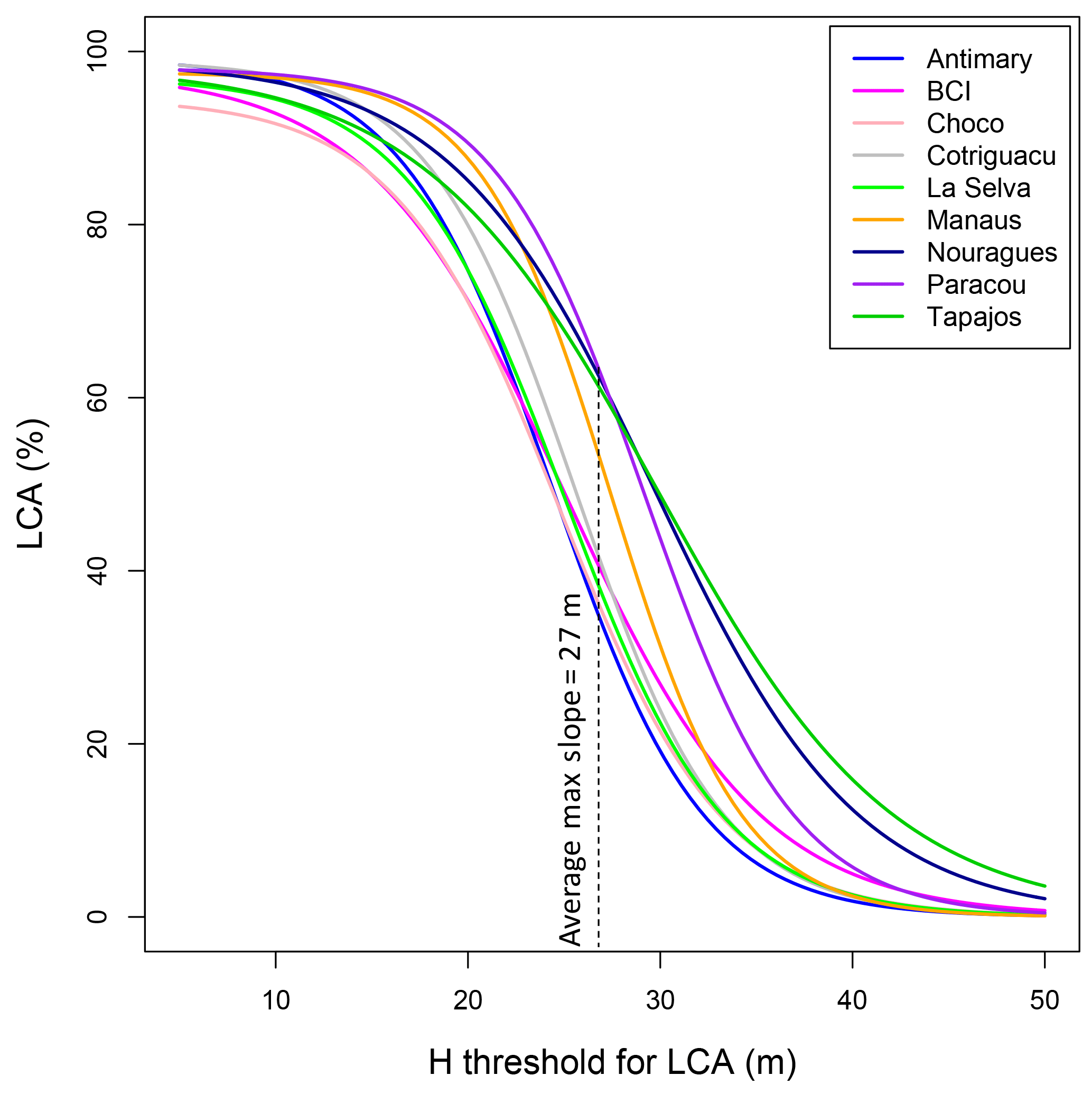
Figure 2 LCA as a function of height thresholds in the nine study sites. The steepest slopes are between 24 m (Antimary) and 30 m (Nouragues), with an average of 27 m across sites. Steepness of slope was obtained by calculating the derivative of the sigmoid models characterizing each site.

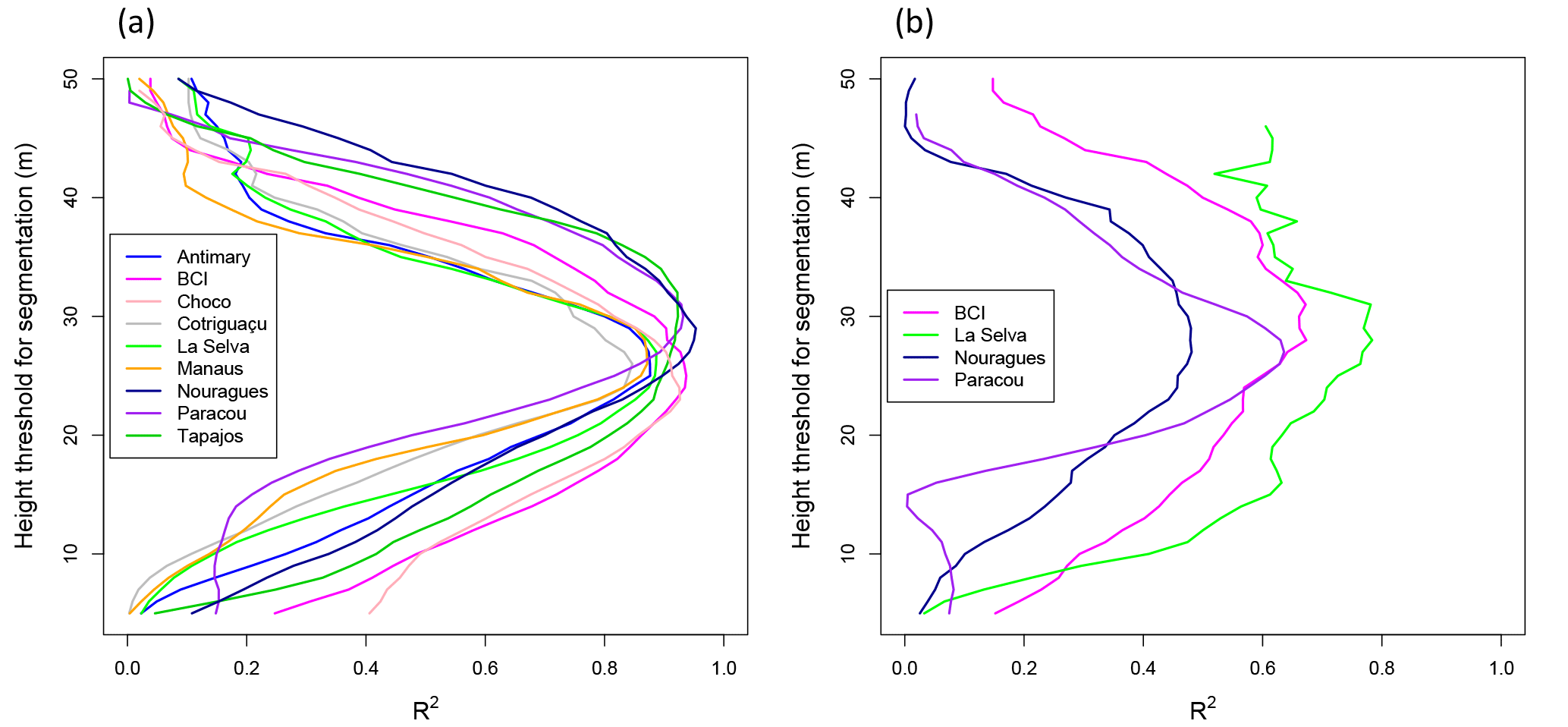
Figure 3 Distribution of R² between tree height thresholds used to determine LCA and AGB_Local in the nine 1 ha subareas (a) and distribution of R² between tree height thresholds and AGB_inv in 1 ha inventory plots of the four calibration sites (b). All optimal thresholds are between 23 and 30 m. The average maximal height threshold is 27 m.

We compared the new approach based on LCA to a similar approach based on MCH, which relies on information on all pixels of an area of interest. In both cases, models were calibrated by using field data from the four calibration sites and their respective mean WD. This comparison is meant to investigate if a metric based on large trees only (LCA) can estimate AGB similarly to a metric that uses information about 100 % of the canopy (MCH).

2.5 Detecting changes in selective logging

Forest degradation due to selective logging is difficult to detect with conventional remote sensing techniques due to the small scale and minor impacts on the forest canopy and biomass compared to severe forest disturbances (e.g., fires, storms or clearing). However, selective logging targets large trees (Pearson et al., 2014) and thus may be detectable using LCA, provided that lidar data are available from pre- and post-logging. Here, we use the Antimary study site that was selectively logged after the 2010 lidar acquisition to examine the use of LCA for detecting logging impacts on the forest canopy and AGB. We apply the large tree segmentation approach on both the 2010 image and on a 2011 post-logging lidar image (see Andersen et al., 2014 for details) to quantify the logging impacts in terms of the distribution of large trees removed from the forest and the loss of AGB.

3 Results

3.1 Inter-site comparison of landscapes and MCH

Topographic variation within the 1 km² images ranged from about 4 m elevation gain in a flat area of Tapajós to steep elevation gain of up to about 100 m in Cotriguaçu and Chocó (Fig. S3). Top canopy height reached up to 60 m, but varies across sites, with Chocó having the lowest MCH (24.1 m) and Nouragues the highest (29.7 m). Forest height in Manaus was more homogeneous than in the other sites, with a standard deviation of 6.8 m for MCH, versus 10.3 m in Paracou. We found no relationship between topography and canopy height, which suggests that variability in forest structure may be due to other ecological and edaphic factors in each site.

3.2 Large canopy area index

The choice of the canopy height threshold impacted LCA more than the minimum number of pixels per cluster (Table S2). The difference due to the choice of the minimal cluster size threshold was on average 1.4 %, calculated as the mean of the difference between the smallest grain (50 pixels) and the largest one (200 pixels) across sites and height thresholds. Based on this analysis, we chose to define LCA using a minimum cluster size of 100 pixels (100 m² for crown area) in the remainder of this study. This corresponds to an area of at least 10 m × 10 m or a circle of approximately 11 m in diameter, consistent with the average crown diameter of large trees of the region (Bohlman and O'Brien, 2006; Figueiredo et al., 2016; David B. Clark, unpublished data).

In contrast, the canopy height thresholds markedly impacted the magnitude of LCA among sites (Figs. 1 and 2, Table S2). As the height threshold increased, intra-site variation in LCA(h) became apparent, showing differences in LCA associated with differences in forest structure (Fig. 1). Tapajós and Nouragues stood out with more area of large trees at the height threshold of 30 m (LCA_30 m=51 and 48 %, respectively) , while Antimary and Chocó showed much lower LCA at this height threshold (LCA_30 m=21 %; Table S2). The steepest slopes of the LCA(h) function corresponded to the highest sensitivity of LCA to height thresholds and the inflection in LCA was found between 24 m in Antimary and 30 m in Nouragues (Fig. 2). The average height of the steepest slope was about 27 m, a value that was used as the optimal threshold across all sites.

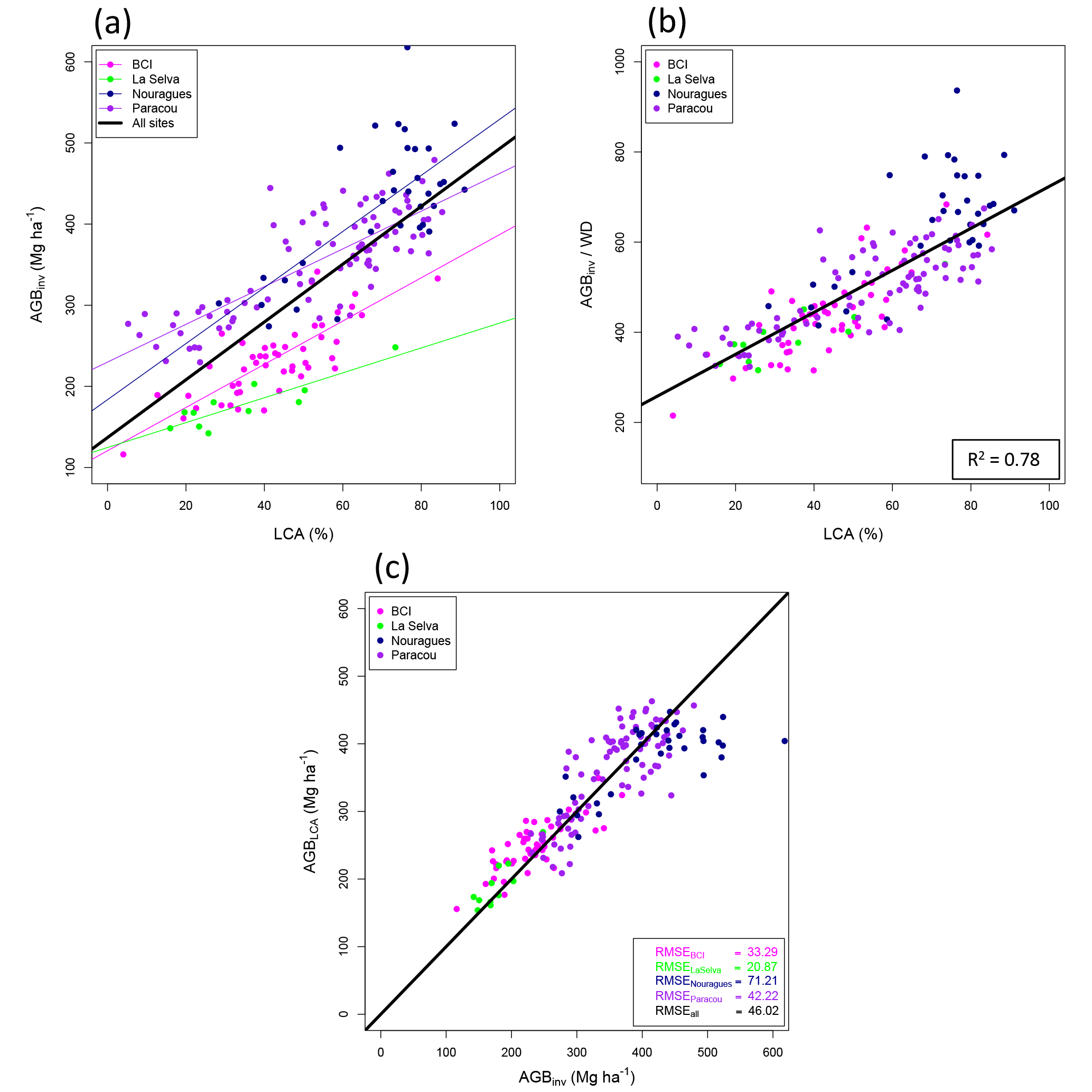
Figure 4 Relationship between AGB_inv and LCA (a), AGB_inv normalized by averaged wood density (WD) (b) and AGB_inv vs. AGB_LCA estimated with the LCA_wd model (c). The black line represents the one-to-one line. Normalizing AGB by averaged wood density (WD) brings the data from different sites closer to a common fit.

Regressing AGB_inv and LCA at the calibration sites (Fig. 3b) showed the best relationships corresponded to height thresholds between 27 m (Nouragues and Paracou) and 28 m (BCI and La Selva), with maximum coefficients of correlation ranging between 0.5 and 0.8. The same analysis repeated using AGB_Local and LCA in the nine sites also confirmed the earlier results that the highest coefficients of correlation between the two metrics occurred between 23 m (Chocó) and 30 m (Tapajós) height thresholds (Fig. 3a), explaining more than 75 % of AGB variation in each site. Based on these results, we defined LCA as the cumulative area of clusters of the canopy height model greater than 27 m height, as the mean of optimal height threshold with highest R² across sites, with clusters covering areas larger than 100 m².

Table 3 Coefficients R², RMSE and bias for the models used to estimate AGB_LCA without and with wood density (WD) as a weighting factor (m_LCA and m_LCA_wd, respectively). cross val. represents cross validation.

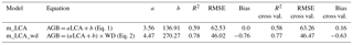
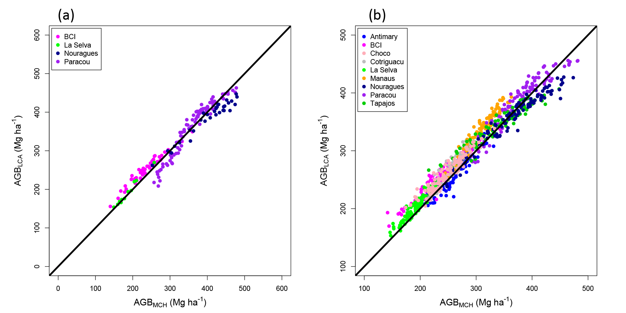
Figure 5 AGB_MCH vs. AGB_LCA in the plots of the four calibration sites (a), and AGB_MCH vs. AGB_LCA in the 1 km² images of the nine sites (b). The black line represents the one-to-one line.

3.3 Variation of AGB derived from LCA

AGB_inv was found to depend linearly on LCA (Eq. 1), with a better coefficient of correlation and RMSE than a power law fit ($R_{\mathrm{linear}}^{\mathrm{2}}=\mathrm{0.59}$, RMSE_linear=62.53 Mg ha⁻¹, vs. $R_{\mathrm{power}}^{\mathrm{2}}=\mathrm{0.54}$, RMSE_power=65.38). Although this model was unbiased (bias_{cross_val}=0.16 Mg), there were clear differences among study sites (Fig. 4a, Table 3). These differences were largely explained by landscape-scale differences in WD, an important factor representing the influence of species composition on the spatial variation in AGB. Since AGB depends on DBH, H and WD (see Chave et al., 2014), average wood volume can be computed approximately as the ratio of AGB divided by the average WD (Fig. 4b). The linear relationship between LCA and wood volume yielded an estimate of the average total volume of forests independently of the site characteristics, through Vol = a LCA + b. Adding more parameters did not improve the performance of the model, except when using WD as a normalizing factor. The two models we retained are therefore of the form of Eqs. (1) and (2):

$$\begin{array}{}\text{(1)}& {\displaystyle }& {\displaystyle }{\mathrm{AGB}}_{\mathrm{LCA}}=a\mathrm{LCA}+b,\text{(2)}& {\displaystyle }& {\displaystyle }{\mathrm{AGB}}_{\mathrm{LCA}}=\left(a\mathrm{LCA}+b\right)\times \mathrm{WD},\end{array}$$

where WD is the mean wood density of a site. The coefficients of the models, as well as their respective coefficients of correlation, RMSE and bias from training data and cross-validation are reported in Table 3.

For AGB estimation, the model based on LCA weighted by WD gives the best result by bringing R² up to 0.78 and RMSE down to 46.02 Mg ha⁻¹ (Fig. 4b, c, Table 3, Eq. 2), with AGB_inv and AGB_LCA falling around a one-to-one line in Fig. 4c. At all sites, RMSE values are between 20.87 and 42.22 Mg, except Nouragues, where RMSE remains large (71.21 Mg) due to high biomass and several outliers from the linear relation. The relationship between LCA and other metrics derived from ground data, such as Lorey's height or basal area, are presented in Sect. S3 and Table S4.

3.4 LCA vs. MCH approach

Finally, we compared these results to AGB estimated using a similar approach based on MCH (AGB_MCH) for the calibration plots (Fig. 5a), and we also compared AGB_LCA to AGB_MCH in all nine sites, using LCA and MCH of the 1 km² images (Fig. 5b).

Both methods perform similarly ($R_{\mathrm{MCH}}^{\mathrm{2}}$ = 0.80, RMSE_MCH = 42.52 Mg ha⁻¹, bias_{cross_val} = −0.21 Mg ha⁻¹; Table S3), showing that relying on a fraction of the lidar information performs as well as using a metric depending on information from all pixels. However, Fig. 5 also shows that the LCA method tends to overestimate AGB compared to the MCH method (bias = 9.66 Mg ha⁻¹), especially in La Selva, BCI, Cotriguaçu and Manaus.

3.5 AGB changes from logging

The impacts of logging on the distribution of large trees and changes in AGB was detected by simply deriving the LCA index from pre- and post-logging lidar data acquired in 2010 and 2011, respectively, in Antimary (Fig. 6). Difference in LCA between the two dates (2010–2011; Fig. 6a) at 1 ha grid cell resolution captured the areas of largest changes in the few months following logging (logging took place between June and November 2011, lidar data were collected in late November 2011). The LCA approach was able to detect an approximately 17 % decrease in LCA, from a mean LCA of 34.8 % in 2010 to 29.2 % in 2011.

The changes were also captured in the frequency distribution of large canopy trees before and after logging (Fig. 6b) and the differences in the spatial distribution (Fig. 6c and d).

These changes in LCA correspond to a biomass loss of 15.2 Mg ha⁻¹ when integrated in Eq. (2) and were of the same magnitude as the planned selectively logging removal rate (12–18 Mg ha⁻¹ or 10–15 m³ ha⁻¹ of timber volume; Andersen et al., 2014). As a comparison, the MCH model led to an estimated biomass loss of 19 Mg ha⁻¹. The difference in the lidar index (ΔLCA) at the native resolution of 1 m (Fig. 6e) was able to capture both the location of all large trees removed from the forest stand and partial regeneration and gap filling that occurred in the forest between the two dates.

4 Discussion

4.1 Inter-site comparisons

Cross-site studies on the structure of tropical forests have led to significant advances in our understanding of tropical forest ecology (Gentry, 1993; Phillips et al., 1998; ter Steege et al., 2006). They have also yielded important insights into new techniques to predict carbon stocks across regions (e.g., Asner and Mascaro, 2014). Comparison of sites in terms of MCH derived for the study sites confirms that there is a strong regional variation in AGB with respect to canopy height, and that east Amazonian sites tend to have much taller trees than central and western Amazonian sites. This was already apparent in the canopy height maps produced by the GLAS sensor (Lefsky, 2010; Saatchi et al., 2011; Simard et al., 2011). Comparing sites in terms of LCA showed a similar pattern of larger trees, being relatively more present in eastern Amazonia, notably in the French Guiana sites and Tapajós. Our most southwestern site was Antimary, in the state of Acre (Brazilian Amazon). However, this site does not represent forests in the western Amazon or the Amazon–Andes gradients with relatively lower WD (Baker et al., 2004) and more fertile volcanic soils impacting the forest structure and dynamics (Quesada et al., 2011). The site in Chocó is also unique in its characteristics because of extremely wet condition and potential disturbance (e.g., selective logging). Additional lidar and ground measurements will allow validating the performance of the LCA in representing the AGB variations in the western Amazon region.

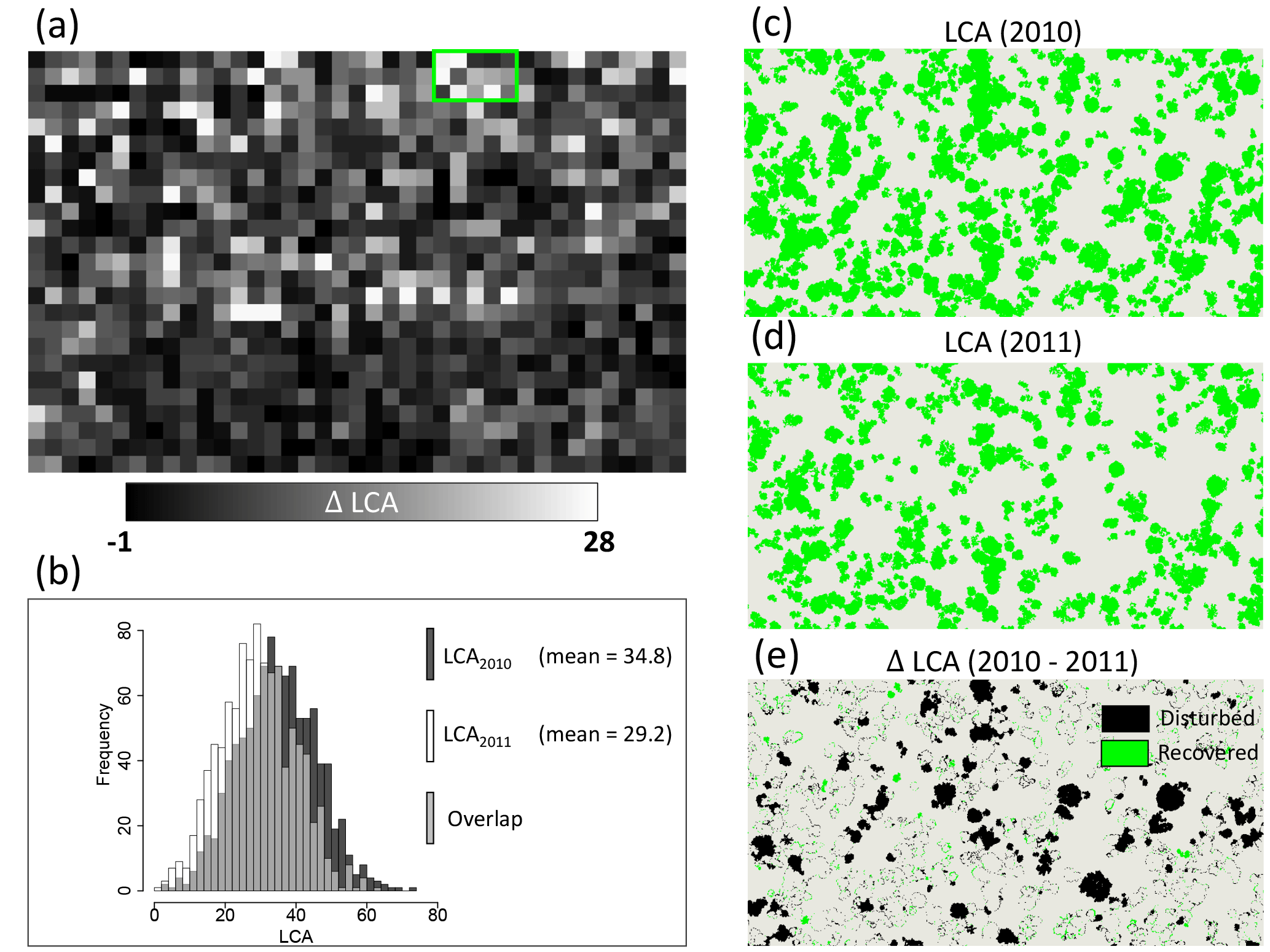
Figure 6 Detection of changes in forest structure from selective logging in the Antimary study area showing (a) the difference between pre- and post-logging (2010–2011) lidar-derived LCA at 1 ha grid cells over the entire study area, (b) the histogram of LCA for the two lidar datasets showing the mean difference and the reduction of medium and large LCA areas from selective logging, (c) 2010 lidar LCA segmentation at 1 m resolution over a sample area in the north of the study site, (d) same LCA segmentation for 2011 lidar data, and (e) difference of the two segmented areas showing the extent of the logging impact on large trees in addition to natural changes in forest structure from changes in canopy gaps from tree falls and tree growth.

4.2 Physical interpretation of LCA

In this study, we introduced a simple structural metric that captures the proportion of area covered by large trees over the landscape (> 1 ha) and explained 78 % of the variation in average forest volume and biomass when weighted by WD in four sites of old-growth Neotropical forests. LCA cannot separate the crown areas of individual trees. However, it is adapted for large-scale monitoring of forest volume and biomass change, as it is a robust and readily accessible metric. For individual tree separation, complex and more computationally intensive approaches are available (Ferraz et al., 2016).

In estimating LCA from lidar data, we examined the spatial clustering properties of LCA and found that the minimum cluster size was less important than the threshold of canopy height, as long as the analysis focused on the relative covered area instead of the density of large trees. We found that using the percentage of the area covered by large canopy trees is an efficient way of overcoming the problem of individual crown segmentation in lidar data. LCA is related to how trees reaching the forest canopy (above a certain height) fill the space and how this characteristic may follow a spatially invariant scaling across tropical forests (West et al., 2009).

Clusters smaller than 100 m² add only a small fraction (1.7 % on average) to LCA values across sites. Including these clusters in LCA would not impact the performance of the model (similar R², RMSE and bias) and would allow us to skip the final steps of the LCA retrieval (see Fig. S2). However, since these pixels either represent single branches reaching above 27 m or the tip of a tree crown, they have no meaning in terms of our LCA metric and do not represent large trees.

LCA provides information on the presence of large trees in a study area, which other metrics such as MCH cannot do. It is an important point, considering that large trees are often the most affected by natural disturbance and targeted by logging companies.

4.3 Correlation between LCA and AGB

The distribution of R² between LCA and AGB for (Fig. 3) is such that the maximum difference in R² between a threshold of 25 and 30 m is approximately 0.1, a negligible value. Hence, AGB retrieval by LCA is relatively insensitive to the height threshold. For most sites, except Antimary, we found a height threshold such that LCA explains about 80–90 % of the variation in AGB or total volume of the forests for each site (60–70 % when compared with ground plots; Fig. 3). Using a height threshold of 27 m for all sites reduced the R² by 0.04 on average (max = 0.08) compared to the optimal height threshold for each site.

Potential differences in MCH among sites are due to footprint size, scan angle and return density (Disney et al., 2010; Hirata, 2004; Hopkinson, 2007; Table 2). However, these effects are generally smaller than the 1 m increment that we used to determine the optimal height thresholds of LCA. As a result, LCA estimation, and therefore AGB inferred from LCA, should depend little on instrument, acquisition and processing (Table 2). This is an important finding given the increasing variety of airborne lidar sensors, and also given the pre- and post-processing methods available for monitoring tropical forest structure and AGB. However, determining whether the 27 m threshold holds for the LCA calculation across the tropics would require a validation at more study studies across continents.

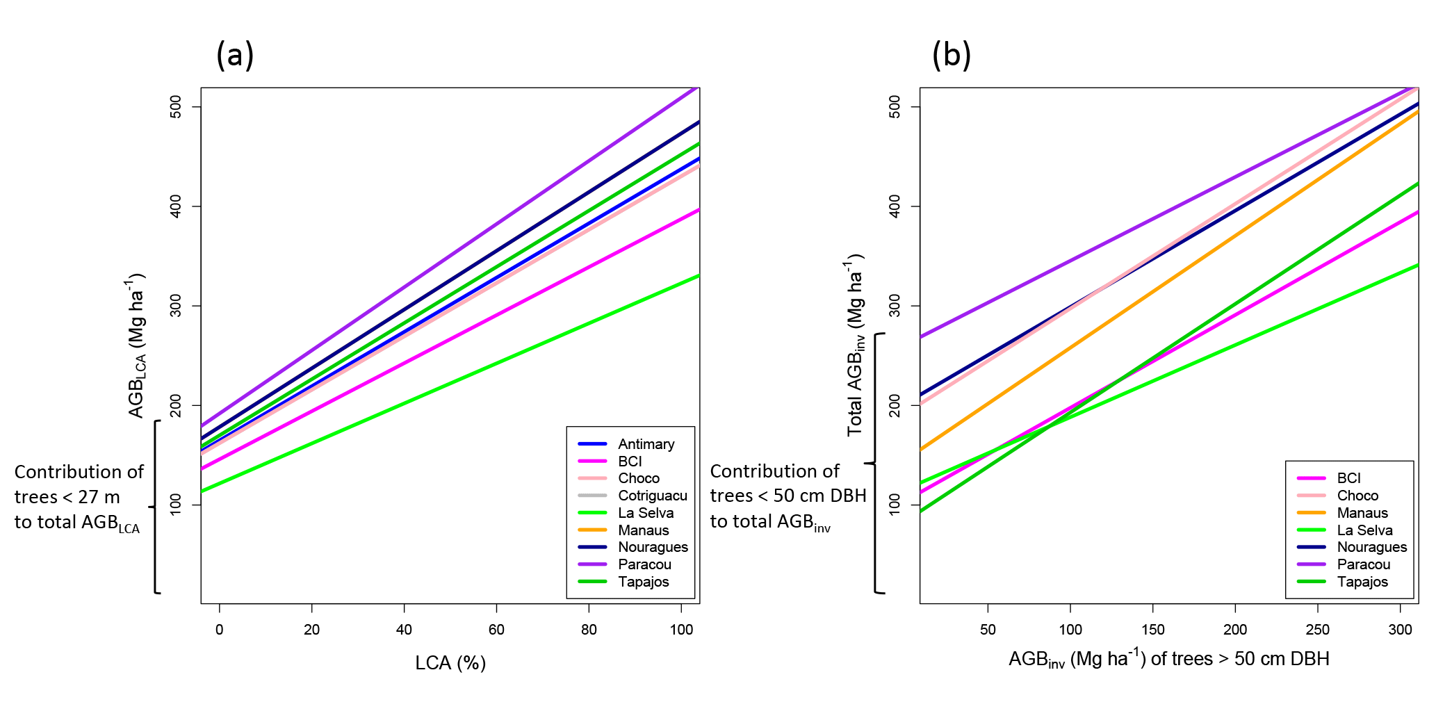
Figure 7 Relationship between LCA and AGB_LCA (a) and relationship between AGB_inv of large trees (> 50 cm DBH) and total AGB_inv (b). In both cases, the intercepts represent the contribution of small trees to total AGB. Note that Manaus and Nouragues overlap because they have the same mean wood density (WD), as well as Chocó and Cotriguaçu.

4.4 LCA relation to ground measurements

The relation between LCA derived from lidar and the ground measurements can be further investigated by converting the 27 m height threshold into equivalent DBH values, using a height–diameter relationship. In the absence of a local DBH–height relation at each site, we made use of the following equation (Chave et al., 2014):

$$\begin{array}{ll}{\displaystyle }\ln \left(H\right)& {\displaystyle }=\mathrm{0.893}-E+\mathrm{0.760}\times \ln \left(D\right)\\ \text{(3)}& {\displaystyle }& {\displaystyle }-\mathrm{0.0340}\times \left(\ln \right(D){)}^{\mathrm{2}},\end{array}$$

where E is a measure of environmental stress for each site that potentially impacts the tree allometry. The corresponding DBH values fall around 35–55 cm, except for Chocó, where the best coefficient of correlation is reached with a DBH threshold of 29 cm (Fig. S4). The average minimum DBH to assign for the definition of large trees that represent variations in AGB is below 50 cm. By choosing a DBH threshold of 50 cm for old-growth undisturbed forests, the LCA model for estimating biomass can have an approximate analog in inventory data. This comparison suggests that the LCA model can also be adjusted with the average WD of trees lager than 50 m, allowing a much faster ground data collection of calibrating the LCA model for different sites (Sect. S4).

A limit to how much LCA can explain variations in AGB relates to forest structure and the AGB of small trees. The lower range of biomass estimation for the LCA model, associated with the intercept for LCA equal to zero, ranged between 122 Mg ha⁻¹ in La Selva and 192 Mg ha⁻¹ in Paracou (Fig. 7a). This lower range identified with the intercept of the LCA–AGB linear model can be interpreted as the AGB associated with all trees smaller than 27 m height (approximately all trees with DBH < 50 cm). Note that the differences between sites are due to differences in their mean WD and not the volume of trees (see Eq. 2 and Fig. 4). Similarly, the contribution of small trees to the total biomass in the ground inventory ranges between around 100 and 200 Mg ha⁻¹, except in Paracou (261 Mg ha⁻¹; Fig. 7b). AGB estimation based on LCA in these sites cannot go under 100 Mg ha⁻¹ or over 500 Mg ha⁻¹. This is not a limitation of the model because LCA is designed to provide AGB estimates for forests reaching at least 27 m in mean canopy height, and such forests generally exceed 100 Mg ha⁻¹ in AGB. Also, the upper threshold of 500 Mg ha⁻¹ is consistent with upper values found globally at 1 ha scale (Brienen et al., 2015; Slik et al., 2013). A recalibration of the method should be envisaged in secondary and highly degraded forests.

4.5 LCA as AGB estimator

The correlation of LCA to AGB_inv suggests that a lidar-based approach can lead to the estimation of AGB at the landscape scale and give useful information on the presence of large canopy trees and their distribution, extending the analysis of large trees in plot-level inventory-based studies (Bastin et al., 2015; Slik et al., 2013).

Therefore, LCA can explain the variations in total forest volume without any ancillary data about the forest or the landscape. Most bias in conversion of LCA to AGB, however, can be corrected across landscapes and sites by scaling the LCA–AGB relationship with average WD at the landscape scale. Our model can therefore potentially be applied to a wide range of forest types, provided that there is information about WD of the study area in the literature.

Wood density has been shown to be a key element of allometric models of AGB estimation (Baker et al., 2004; Brown et al., 1989; Chave et al., 2004; Nogueira et al., 2007). If WD is assumed to be constant across DBH classes, the mean WD at the plot scale can readily be used to scale LCA to biomass. However, if the WD of large trees is smaller or larger than the average WD, (e.g., in BCI and Chocó: Sect. S4, Fig. S5), the use of mean WD to scale LCA may introduce a slight bias in biomass estimation. A difference in mean WD of 0.1 g cm⁻³ would introduce a bias of ±10 % in the biomass estimation when using our model. We found that using mean WD of large trees or basal-area-weighted WD instead can give slightly better results and could circumvent the differences in size distribution of the WD (Sect. S4). Instead we could rely on the WD of large trees only. This would make the collection of ground data easier and cost effective for biomass estimation, because trees ≥ 50 cm DBH only represent 5–10 % of the stems of a plot (Sect. S4, Fig. S6). Focusing on the WD of dominant or hyper-dominant species could also be an alternative approach for future use of lidar-derived LCA for large-scale biomass estimation (Fauset et al., 2015; ter Steege et al., 2013). In the absence of information on WD from the literature, modeled WD could potentially be used, but would give greater errors. These errors should be taken into account when reporting on the uncertainty in the results.

4.6 LCA and MCH

The comparison of LCA and MCH metrics showed that both performed similarly in estimating AGB, highlighting the importance of large canopy trees to estimate biomass. The differences between the two methods in estimating AGB show that two methods can have similar performance in terms of R² and RMSE and nonetheless lead to different estimations, with LCA giving higher AGB estimations in some sites. The choice of a metric is therefore crucial to estimate AGB, especially when estimating the changes in biomass (see Sect. 4.7).

Both MCH and LCA–AGB models performed relatively poorly in high biomass plots of the Nouragues study area, by underestimating biomass values greater than 500 Mg ha⁻¹ (Figs. 4 and 5). To explain the underestimation, we performed three tests. (1) We examined the differences in the ground estimated biomass values with and without tree height and found no significant impact in reducing the effect of underestimation. (2) We tested the hypothesis that the height threshold used for LCA estimation across sites was not suitable for the Nouragues study site and dismissed the hypothesis because 27 m was found to be the optimum threshold for Nouragues plots. (3) We examined the errors in the lidar estimation of forest height and found that except for an extremely high AGB_inv of 617 Mg ha⁻¹, the four other high biomass outliers are all located in the 6 ha Pararé plot located on a very steep topography. The lidar DTM of this area shows an average within-plot elevation range of 90 m. Ground detection on steep terrain can be erroneous, depending on the lidar point density and the view angle, causing large area interpolation errors for DTM development and significant error in canopy height measurements (Leitold et al., 2015). Other factors that may affect the underestimation of AGB by LCA or MCH in the Nouragues site may be due to the presence of forest patches with clusters of large trees and overlapping crown areas. It is also possible that the relationship between AGB and LCA is not linear for very high AGB values. This could be tested in the future with a larger number of sites with very high biomass.

4.7 LCA and forest degradation

Although LCA and MCH may perform similarly in capturing the forest biomass variations and changes, the use of LCA in detecting forest degradation and logging is more straightforward because of its relation to large trees. The LCA approach was able to accurately detect changes in forests after logging by locating where the large trees are extracted. Our estimate of biomass change from the LCA approach was higher than the biomass loss of 9.1 Mg ha⁻¹ reported by another study using the 25th percentile height above ground as the lidar metric for biomass estimation (Andersen et al., 2014). It can be expected that relying on the 25th percentile height metric for biomass estimation would place more emphasis on the lower part of the canopy (understory) that is either less damaged or has gone through some level of regeneration after logging. Models based on LCA or MCH, on the other hand, may be more realistic for estimating AGB changes because they capture the changes in large trees and upper forest canopy structure that contain most of the biomass and are directly impacted by logging and biomass removal.

The higher biomass loss estimation from the MCH model (19 Mg ha⁻¹) again shows how different metrics can lead to different results. Here, three methods based on three different lidar metrics yielded results that differed by more than twofold. LCA could become an important tool to detect forest degradation, in particular selective logging, considering that large trees are targeted by logging companies.

4.8 Future applications of LCA

The LCA definition in our study relies on the high-resolution information of forest height, allowing for the detection of crown area of large canopy trees. Can a similar measure be derived from large footprint lidar observations such as the future NASA spaceborne lidar mission GEDI (Global Ecosystem Dynamic Investigation)? GEDI will not provide spatially continuous data on forest height, but its footprint size (∼ 25 m) and dense sampling may be adequate to develop statistical indicators of large trees over the landscape.

Similarly, future spaceborne radar missions could also provide useful information to retrieve large canopy areas. The synthetic aperture radar (SAR) tomographic observations of the European Space Agency (ESA) Biomass mission will provide wall-to-wall imagery of canopy profile that could be converted to LCA over the landscape (Le Toan et al., 2011). Preliminary research based on airborne TomoSAR measurements has already shown that backscatter power at about 30 m above the ground, with sensitivity to the distribution of large trees, explained the variation in AGB over Nouragues and Paracou plots better than the backscatter power related to the lower part of the canopy (0–15 m; Minh et al., 2016; Rocca et al., 2014). Future research on exploring the use of an equivalent radar index product from Biomass height or tomography measurements at a height threshold (e.g., 27 m) may provide a potential algorithm to map the area of large trees and estimate forest volume and biomass changes across the landscape.

5 Conclusions

We introduce LCA as a new lidar-derived index to capture the variations in large trees and total volume and biomass across landscapes that remain spatially and regionally invariant. The importance of LCA is in its relevance to the structure and ecological characteristics of large trees in filling the canopy space and their unique contribution in determining the total volume and biomass of forests. Unlike other lidar-derived metrics, LCA is linearly related to total AGB after being weighted by average WD. This linear relationship remains unique across different forest types, making the LCA model broadly applicable. The comparison of the LCA index with ground plots suggests that DBH > 50 cm is a more reliable threshold to quantify the number and distribution of large trees in undisturbed old-growth tropical forests and in capturing the variations in the total AGB across landscapes and regions. The results of our study may encourage further research in the use of lidar data for detecting the distribution of larger trees in tropical forests for ecological and conservation studies.