the Creative Commons Attribution 4.0 License.
the Creative Commons Attribution 4.0 License.
 | 18 Jan 2018
An enhanced forest classification scheme for modeling vegetation–climate interactions based on national forest inventory data
Stephanie Eisner
Rasmus Astrup
Jonas Fridman
Ryan M. Bright
Forest management affects the distribution of tree species and the age class of a forest, shaping its overall structure and functioning and in turn the surface–atmosphere exchanges of mass, energy, and momentum. In order to attribute climate effects to anthropogenic activities like forest management, good accounts of forest structure are necessary. Here, using Fennoscandia as a case study, we make use of Fennoscandic National Forest Inventory (NFI) data to systematically classify forest cover into groups of similar aboveground forest structure. An enhanced forest classification scheme and related lookup table (LUT) of key forest structural attributes (i.e., maximum growing season leaf area index (LAImax), basal-area-weighted mean tree height, tree crown length, and total stem volume) was developed, and the classification was applied for multisource NFI (MS-NFI) maps from Norway, Sweden, and Finland. To provide a complete surface representation, our product was integrated with the European Space Agency Climate Change Initiative Land Cover (ESA CCI LC) map of present day land cover (v.2.0.7). Comparison of the ESA LC and our enhanced LC products (https://doi.org/10.21350/7zZEy5w3) showed that forest extent notably (κ = 0.55, accuracy 0.64) differed between the two products. To demonstrate the potential of our enhanced LC product to improve the description of the maximum growing season LAI (LAImax) of managed forests in Fennoscandia, we compared our LAImax map with reference LAImax maps created using the ESA LC product (and related cross-walking table) and PFT-dependent LAImax values used in three leading land models. Comparison of the LAImax maps showed that our product provides a spatially more realistic description of LAImax in managed Fennoscandian forests compared to reference maps. This study presents an approach to account for the transient nature of forest structural attributes due to human intervention in different land models.
- Article
(7198 KB) - Full-text XML
-
Supplement
(377 KB) - BibTeX
- EndNote


The structural properties of a forest largely determine the amount of mass, energy, and momentum exchanged with the atmosphere contributing to weather and climate on multiple scales (Bonan, 2008). Given their controls on photosynthesis, albedo, and evapotranspiration, structural attributes like canopy leaf area and tree heights are crucial variables in modeling carbon, water, and energy fluxes in forests. Leaf area index (LAI, defined as the hemisurface area of foliage per unit horizontal ground surface area; Chen and Black, 1992) is considered an essential climate variable (ECV; GCOS, 2012) as it quantifies the areal interface between the land surface and the atmosphere, hence representing a control over the exchange of mass and energy between the terrestrial biosphere and the atmosphere (Bonan, 2015). Similarly, canopy top and bottom heights, ztop and zbottom, are important variables required for calculating roughness length and displacement height that largely determine aerodynamic resistances to heat, moisture, and momentum transfer (Oke, 2002). In land models, land surfaces are often classified by the main aggregate land cover (LC) classes: vegetation, urban, inland water, bare soil, and ice – typically with the assistance of optical satellite remote sensing (Friedl et al., 2002; Hansen et al., 2000; Poulter et al., 2015). The vegetation LC class is further divided into a number of subclasses according to their biophysical properties, grouping them into what is often termed plant functional types (PFTs) or “broad groupings of plant species that share similar characteristics (e.g., growth form) and roles (e.g., photosynthetic pathway) in ecosystem function” (Wullschleger et al., 2014). LC maps are converted into PFT maps using various model-dependent algorithms (e.g., Lawrence and Chase, 2007; Reick et al., 2013) or “cross-walking” tables (e.g., ESA LC, 2017, manual p. 75; Poulter et al., 2015).
Differences in forest structure within a given LC type (or PFT) can differ substantially (Kuuluvainen et al., 2012; Newton, 1997), and preserving within-LC (or within-PFT) differences in forest structure is necessary for more accurate modeling of surface fluxes in forests. While some land models assimilate local information on present day forest structure from satellite remote sensing to account for within-PFT variation (e.g., Community Land Model 4.5, CLM4.5, Oleson et al., 2013; Jena Scheme of Atmosphere Biosphere Coupling in Hamburg, JSBACH, Reick, 2012), future structure must still be prescribed. Because land use transitions in modeling simulation studies of anthropogenic LC change are often represented by a change in PFT area in land models, post-disturbance changes to structure within forest PFTs go undetected (Lawrence et al., 2012; Reick et al., 2013). Hence, a forest classification that accounts for major variation in key structural attributes, such as LAI or canopy height, may lead to better predictions of surface fluxes in forests, not only in studies of prescribed land cover and/or management change, but also for dynamic vegetation studies that rely on fixed PFT parameters obtained from lookup tables (LUTs). The time-invariant nature of the fixed parameter LUTs may be avoided by increasing the number of forest classes within a single forest PFT with sufficient differentiation in key structural attributes (i.e., from young to mature forests). In addition to grouping forests according to their shared phenological characteristics, further grouping according to their structural characteristics (i.e., accounting for the effects of forest management) would strengthen prediction confidence in intensively managed regions.
LC data needed by land models should ideally be representative of sufficiently large areas because incorporating fragmented data stemming from individual research sites and individual research experiments is limited by available computing resources and rapidly increasing model complexity. Most countries are currently conducting National Forest Inventories (NFIs) to quantify the extent and amount of forest resources with standardized reporting for compiling global Forest Resources Assessments (FRAs; e.g., FAO, 2015). NFI data have previously been used in research aiming to attribute climate effects to management activities because they reflect the human influence on forest structure (Bright et al., 2014; Naudts et al., 2015, 2016). However, as NFI data characterize only forested areas, other LC data are needed to form the complete surface representation required by land models. The state-of-the-art LC products, such as the European Space Agency (ESA) Climate Change Initiative (CCI) LC product (ESA LC, 2017), allow for cross-walking from LC classes to PFTs used in land models. It is noteworthy that ESA LC products have high spatial resolution (0.003∘) compared to the common global grid sizes (e.g., 0.5–1∘) used in land models, which allows for more flexibility in cross-walking and LC data aggregation.
In this study, we develop a forest classification scheme based on NFI data to better characterize the transient nature of forest key structural attributes to provide more realistic starting values for different land model simulations. We develop our concept using NFI data from Fennoscandia as it represents one of the most intensively managed forested regions of the world (e.g., Kuuluvainen et al., 2012). From the perspective of climate modeling, NFI data are well suited for enhancing the structural description of forests in global LC datasets because similar data are available for most developed countries and new data are collected systematically. The aims of this study are to (1) develop a semi-objective clustering analysis approach to come up with an LC-dependent structural LUT, which reflects the transient nature of the key forest structural attributes in managed forests, (2) create a new forest LC product for Fennoscandia based on multisource NFI (MS-NFI) data to allow for the spatial application of the LUT of key structural attributes, (3) augment the new forest classification by importing non-forest LC classes of the ESA LC product to form the complete surface representation required by land models, (4) compare the forest extent of the new LC product with the original ESA LC product to point out geographic areas where the largest differences occur to provoke discussion on alternative information sources for parameterizing land models, and (5) visualize and compare maps of our maximum growing season LAI (LAImax) with reference LAImax maps produced using the ESA LC product, a model-generic cross-walking table (Poulter et al., 2015), and PFT-dependent LAImax values used in three land models: JSBACH, Joint UK Land Environment Simulator (JULES), and Organizing Carbon and Hydrology in Dynamic EcosystEms (ORCHIDEE).
2.1 Data
2.1.1 NFI plot data
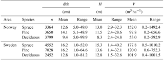
Norwegian NFI data (Tomter et al., 2010) from 2007 to 2015 and Swedish NFI data (Fridman et al., 2014) from 2011 to 2015 were used in this study. NFI employs a network of field plots from which trees are measured and growth is monitored systematically. NFI data are systematically collected and processed by forest authorities and are used to quantify the amount and extent of forest at a national level. The diversity in forest structure throughout the Fennoscandian region is well represented in the Swedish and Norwegian NFI data. The Norwegian NFI contained data from 10 813 circular 8.92 m radius sample plots (250 m2), while the Swedish data were from 14 032 circular 10 m radius sample plots (314 m2). Plots that were divided (i.e., not completely circular) or that did not have trees were excluded from the data prior to the analysis. The main tree species of the area are Norway spruce (Picea abies (L.) H. Karst.), Scots pine (Pinus sylvestris, L.), and silver and downy birches (Betula pendula Roth and pubescens Ehrh.). Monocultural plots of birch are rare, but birches are common in plots with different species mixtures. Plot data were classified as spruce-, pine-, or deciduous-dominated (contains also other tree species) forests based on species with the largest share of total stem volume (m3 ha−1) on the sample plot (Table 1.).
Table 1Descriptive statistics for the National Forest Inventory (NFI) data. Abbreviations: n is the number of sample plots, dbh is diameter at breast height, H is basal-area-weighted mean tree height (i.e., Lorey's height), and V is total stem volume.
2.1.2 MS-NFI data
NFI plot characteristics are extrapolated for areas between the NFI plots using the non-parametric k–nearest-neighbor (kNN) estimation method (e.g., Tomppo et al., 2014). The extrapolation step is called multisource NFI (MS-NFI) because it employs data from different remote sensing systems (i.e., satellite and aerial platforms) and NFI plots. MS-NFI applies high-spatial-resolution (< 900 m2) satellite images to separate forested areas from other LC classes and digital terrain models to correct topographical distortions. In Fennoscandia, the common stand size is only 1–2 ha (i.e., landscape is fragmented by forests with different development stages) and thus high-spatial-resolution satellite products are needed to prepare the MS-NFI maps. All processing of the MS-NFI data is done by forest authorities. MS-NFI maps are typically provided for forest variables such as Lorey's height (i.e., basal-area-weighted mean tree height) (H, m), forest stand age (years), and stem volume (V, m3 ha−1) by species. The newest MS-NFI maps for Finland (of 2013) and Sweden (of 2010) were downloaded from the Natural Resources Institute Finland (LUKE) portal (LUKE, 2016) and from the Swedish University of Agricultural Sciences (SLU) portal (SLU, 2016). For Norway, MS-NFI data (compiled during the first decade of the twenty-first century) called “SAT-SKOG” (Gjertsen, 2007, 2009) and a forest resource map called “AR5” (Ahlstrøm et al., 2014) were used to obtain all required inputs and coverage of the northernmost forest areas (i.e., Finnmark county; Supplement S1).
2.1.3 ESA LC product
The ESA LC-product series contains a set of annual maps from 1992 to 2015 (ESA LC, 2017). The product series follows processing in which a baseline LC product is applied; although the annual maps are not fully independent from each other, they are temporally consistent. The baseline LC product was based on MERIS FR and RR archive between the years 2003 and 2012 and was back-dated and updated based on data from other satellite sensors (AVHRR between 1992 and 1999, SPOT-VGT between 1999 and 2013, and PROBA-V between 2013 and 2015). In this study, the newest 2015 (v.2.0.7) LC product was used as it is more likely to be used by land modelers. This LC-product version has been validated against GlobCover 2009 reference data (cf. p. 39 in the product manual ESA LC, 2017). The spatial resolution of the ESA LC product is ∼ 0.003∘, and it follows standardized hierarchical classification by the United Nations Land Cover Classification System (UN-LCCS), which allows for the conversion of LC classes into PFTs based on a cross-walking table (ESA LC, 2017, manual p. 75; Poulter et al., 2015). The 2015 ESA LC product contains three LC classes to describe forests in Fennoscandia: broadleaved deciduous (60–62), needleleaved evergreen (70–72), and mixed broadleaved and needleleaved (90; ESA LC labels in parentheses). The second label digit from the left is designed to indicate forest fraction within an LC pixel: the canopy is “closed” when the forest pixel cover fraction is > 40 % (labels 61 and 71) and “open” when the forest pixel cover fraction is between 15 and 40 % (labels 62 and 72). Labels 60 and 70 are used to indicate that the within-pixel forest fraction is more than 15 %, but it is not known whether that pixel is closed or open. The 2015 ESA LC product for Fennoscandia contained only classes 60, 61, 70, and 90 (i.e., no pixels were assigned to subclasses 62, 71, or 72).
2.2 Methods
2.2.1 Forest classification scheme
NFI data were first used to develop the forest classification scheme based on four key forest structural attributes: total stem volume (V), Lorey's height (H), crown length (CL), and LAImax (LAImax calculation is described in Supplement S2; Fig. 1). V defines species dominance, H corresponds with the aerodynamic height or ztop (Nakai et al., 2010), CL is needed to estimate canopy bottom height or zbottom (i.e., zbottom= H – CL; modeling of CL described in Supplement S3), and LAImax quantifies the exchange surface area between the land surface and the atmosphere. First, a clustering analysis of the NFI data was used to find medoids of the four-dimensional (4-D) V–H–CL–LAImax clusters because forest variables are not independent from each other. After defining the 4-D cluster centers, another Euclidean-distance-based classifier was used to define the 4-D cluster boundaries in order to apply the classification on MS-NFI data. An overview of the analysis is shown in Fig. 1.
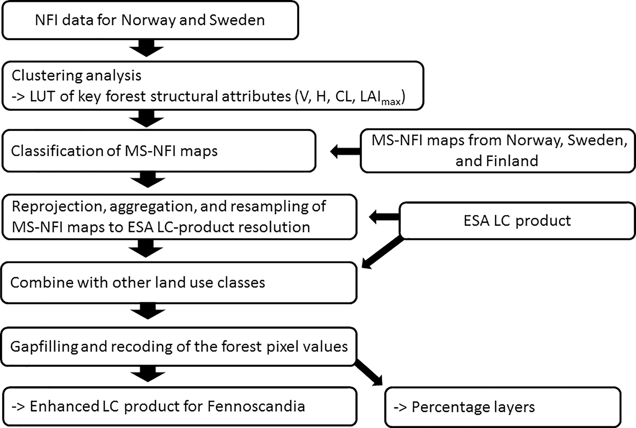
Figure 1Flowchart for developing and applying the forest classification scheme (Sects. 2.2.1 and 2.2.2). Abbreviations: National Forest Inventory (NFI), lookup table (LUT), total stem volume (m3 ha−1) (V), Lorey's height (H), crown length (CL), maximum growing season leaf area index (LAImax), multisource NFI (MS-NFI; i.e., products provided by forest authorities), European Space Agency Land Cover (ESA LC) product.
The Norwegian and Swedish NFI data were merged and grouped into species groups (i.e., spruce, pine, and deciduous dominated) to account for differences in forest structural properties. First, the optimal number of structural subgroups within each species group (i.e., spruce, pine, deciduous) was analyzed. The optimal number of clusters was assessed by plotting the curve between the total within-cluster sum of squares (wcss) and the number of clusters (k) and then observing around which k the relationship resembles a “bent knee” (i.e., the “elbow method”; Ketchen Jr. and Shook, 1996). Analysis was run using the R package “factoextra” (Kassambara and Mundt, 2017). In each species group the bent knee was located between k= 3 and k= 5, and thus the optimal k was set to 4 (i.e., the number of structural subgroups was set to four). Then, using the predefined number of structural subgroups (k= 4) within each species group (n= 3), a k-medoids clustering analysis was used to define the cluster “centroids” (i.e., medians) within the V–H–CL–LAImax space to form a LUT of the key forest structural attributes ( 12 forest classes). The k-medoids algorithm is a data partitioning method in which each cluster is represented by one of the cluster objects (i.e., all subgroup LUT values (V, H, CL, and LAImax) are from the same plot; Kaufman and Rousseeuw, 1990). The k-medoids algorithm assigns all plots to the nearest cluster centers and calculates the wcss. New cluster centers are updated and the plots are reassigned. Cluster centers are adjusted iteratively until they do not change. The k-medoids algorithm was chosen because only the number of clusters is required as an input and also because it is robust against outliers. The analysis was run using the “cluster” package in R (Maechler, 2017).
A method to assess cluster boundaries was needed because many plots were located near the edges of the 4-D clusters. We chose to determine cluster boundaries using V and H since these are often available for large geographical areas from MS-NFIs. Mahalanobis (1936) distance (MD) was used to quantify the within-cluster variation in the V and H space (i.e., V–H space) because it corresponds to the Euclidean distance after V and H have been normalized. MD is a multidimensional method to determine how many standard deviations a data point is away from the class mean. For MD calculation the cluster mean values were obtained based on the 4-D (i.e., V, H, CL, and LAImax) and not in 2-D (i.e., V and H) clusters, and thus the cluster boundaries are not circular. MD values were calculated for each species group and the respective subgroups. The binning (i.e., grid of 14 × 14) interval of the V–H space was set subjectively to add resolution on younger forest structures. For each grid cell and for each subgroup, a median MD value was calculated. To represent results using a grid surface, the cell was assigned to a subgroup with the smallest median MD.
2.2.2 Compiling the enhanced LC product
In order to apply the newly developed LUT, the most recent MS-NFI maps from Norway, Sweden, and Finland were used to classify the Fennoscandian forests into the 12 forest classes (i.e., the forest LC product was developed). MS-NFI data were classified as spruce, pine, or deciduous dominated based on species with the largest share of pixel total stem volume (m3 ha−1). The share of tree species other than pine or spruce was assigned to the deciduous group. After the species group was assigned, a gridded V–H space was used to determine pixel subgroup. Possible V–H combinations without MD value (i.e., falling outside the V–H space) were assigned to the closest subgroup based on V. After classifying all data, the forest classes were recoded as integers between 1 and 12 (i.e., three species groups × four structural subgroups).
The classified MS-NFI maps were reprojected, aggregated, and resampled to complement the ESA LC product (v.2.0.7; ESA LC, 2017) to form the complete surface representation required by land models. Two types of aggregation routines were used for upscaling: forest class was assigned based on mode (among the 12 forest classes) and within-pixel forest cover fraction based on mean (for this purpose, forested pixels in MS-NFI data were recoded as 100 and other pixels as 0). In other words, for each forested ESA LC pixel (∼ 90 000 m2), forest class and within-pixel forest cover fraction (%) were obtained based on classified MS-NFI maps (∼ 260 or ∼ 630 m2). Two exceptions occurred: (1) if the ESA LC pixel was not classified as forest but the MS-NFI maps indicated the presence of forest, and (2) if the ESA LC pixel was classified as a forest but MS-NFI maps indicated non-forest. For pixels that were classified as forest by the ESA LC product but the forest cover fraction within that pixel in the enhanced LC product did not exceed the 15 % threshold (i.e., definition used by the ESA LC product) according to the MS-NFI data, forest class was assigned based on moving average interpolation (referred to as “gapfilling”). Gapfilling was necessary because land (climate) models require completeness in LC to resolve computations of mass, energy, and momentum fluxes (note: gapfilled pixels are coded separately, which allows them to be either included in or excluded from analysis). Non-forest LC classes were imported from the ESA LC product to supplement our forest pixels.
To allow for more flexible cross-walking or aggregation to a lower spatial resolution in the preparation of surface datasets in land models, for each forest LC pixel, coverage fractions (referred to as “percentage layers”) for each of the 12 forest classes were calculated (i.e., 12 layers with values ranging between 0 and 100 based on subgroup abundance within the ESA LC pixel). In addition, gapfilled pixels and non-forest LC classes are provided as own layers. These layers also allow more flexibility for modelers in choosing the number of desired input land cover classes (i.e., modelers may use, for example, the three most abundant forest classes instead of keeping to the most abundant one). Raster analyses were performed using the “rgdal” (Bivand et al., 2017) and “raster” (Hijmans, 2017) packages in R. The enhanced LC product for Fennoscandia, including the percentage layers, can be downloaded from Majasalmi et al. (2017).
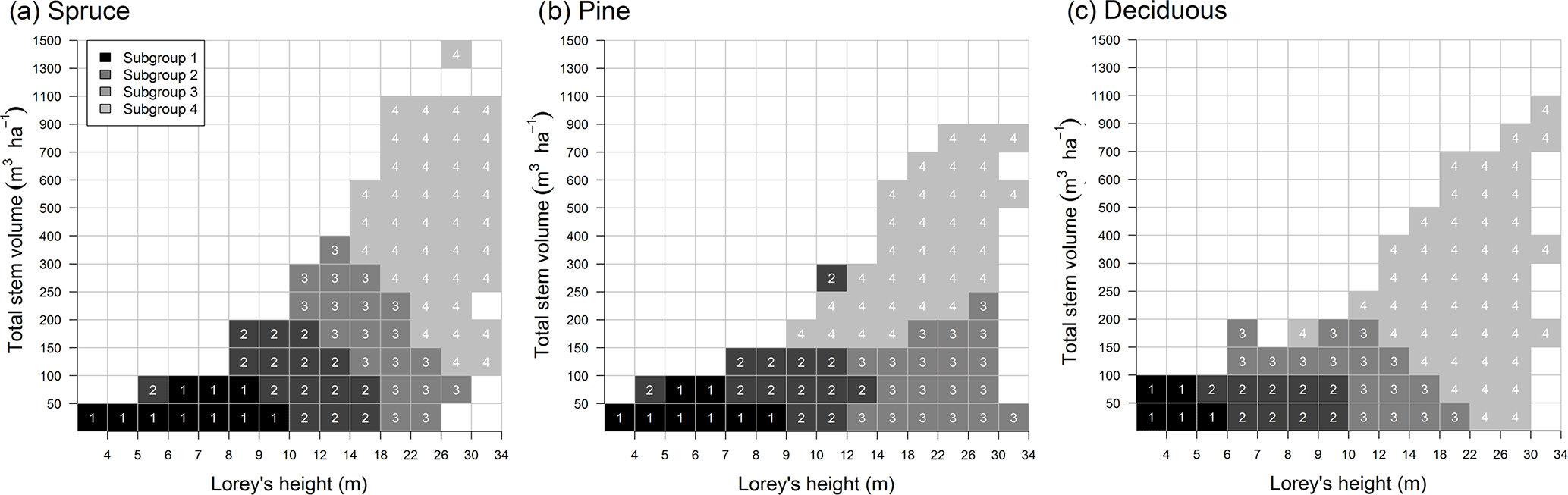
Figure 2Gridded representation of vegetation subgroups, i.e., (a) spruce, (b) pine, and (c) deciduous, within the total stem volume (V) and Lorey's height (H) space (referred to as V–H space) based on NFI data. Visualization is required to map subgroup distribution in V–H space and is used to apply the classification to the MS-NFI maps.
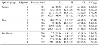
Table 2A forest classification scheme lookup table (LUT). Abbreviations: V is total stem volume (m3 ha−1), H is Lorey's height (m), CL is crown length (m), and LAImax is maximum growing season leaf area index (m2 m−2). The “Recoded label” column is a key to be used with the enhanced CL product. Interquartile range (i.e., first quartile subtracted from the third quartile) is given inside parentheses.
2.2.3 Comparison of the LC products
To highlight areas where the forest extent differed the most, a difference map between the enhanced “back-classified” (i.e., into ESA LC classes) map and ESA LC product was calculated using ∼ 0.3∘ resolution. This resolution was chosen as it represents a good compromise between higher-resolution regional modeling (0.05–0.1∘) and coarser-resolution regional and global modeling (0.5–1∘). In addition, LC-class changes (e.g., from cropland to conifer forest) were quantified using a confusion matrix between the ESA LC classes and enhanced back-classified map classes in the original product resolution (∼ 0.003∘). The back-classification was done using the percentage layers of different forest subgroups: if > = 70 % of the MS-NFI pixels within the ESA LC pixel were classified into the conifer or deciduous group, the pixel was classified as “needleleaved” (class 70) or “broadleaved” (class 60), but otherwise it was classified as “mixed” (class 90). The difference map was calculated after both products (i.e., the enhanced back-classified map and the ESA LC product) were aggregated to ∼ 0.3∘ resolution using pixel modes. The LC class changes are presented with a confusion matrix between the ESA LC product and the enhanced back-classified map; each row of the matrix represents an occurrence in the enhanced back-classified map, while each column represents the respective occurrence in the ESA LC product. The percentage of pixels belonging to the same LC class in both products is shown in diagonal, whereas percentage values outside the diagonal quantify the change (“confusion”) between the different LC classes. The confusion matrix was calculated using the “caret” package (Kuhn, 2008) in R.
2.2.4 Comparison of LAImax maps
To demonstrate the potential of our LC product to provide more realistic LC-dependent values of key forest structural attributes for forested areas in Fennoscandia, we compared our LAImax map (i.e., produced using enhanced LC product and related LUT) with reference LAImax maps produced using the ESA LC product, a model-generic cross-walking table (Poulter et al., 2015), and PFT-dependent LAImax values used in ORCHIDEE, JULES, and JSBACH. Only forested pixels were used for demonstration.
According to an ESA LC cross-walking table (Poulter et al., 2015), a pixel classified as broadleaved deciduous trees (BDTs) is assumed to contain 70 % BDTs, 15 % broadleaf deciduous shrub (BDS), and 15 % natural grass. A pixel with needleleaved evergreen trees (NETs) is defined to comprise 70 % NET, 5 % broadleaf evergreen shrub (BES), 5 % broadleaf deciduous shrub (BDS), 5 % needleleaf evergreen shrub (NES), and 15 % natural grass. As all the required shrub LUT values were not available, the percentage of BDS was set to 15 % for NET (i.e., equivalent to BDT weights). For a mixed-leaf-type forest (ESA LC class 90), the estimates were obtained as an average of BDT and NET values because all the required input data (e.g., values for needleleaf deciduous tree (NDT) and BES) were not available to follow the ESA LC-product cross-walking scheme.
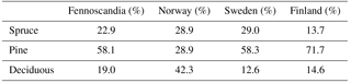
Table 3The percentage (%) of forest pixels (i.e., excluding gapfilled pixels) belonging to different species groups in the enhanced LC product (referred to as Fennoscandia) and separately for each country (the spatial distribution of different forest subgroups and their frequency distributions are shown in Fig. 3). Values are based on MS-NFI data.
JULES, JSBACH, and ORCHIDEE LUTs employ PFT-dependent LAImax values. In JULES according to Clark et al. (2011), the PFT-dependent LAImax values are 9 for a broadleaf tree (BDT), 5 for a needleleaf tree (NET), 4 for a C3 grass (natural grass), and 3 for a shrub (BDS; acronyms used by the ESA LC cross-walking table in parenthesis). In ORCHIDEE as reported by Lathière et al. (2006), the respective PFT-dependent LAImax values are 4.5 for both boreal BDT and NET, and 2.5 for a C3 grass (same LAImax also used for BDS). In JSBACH according to Schürmann et al. (2016), the PFT-dependent LAImax value was 5 for extratropical deciduous trees (BDTs), 1.7 for coniferous evergreen trees (NETs), and 3 for C3 grass (same LAImax also used for BDS).
3.1 Forest classification scheme
As a result of our classification scheme, a LUT of the key structural variables (i.e., V, H, CL, and LAImax) was created (Table 2.). The boundaries of the subgroups were determined based on MD, which can be visualized using a gridded representation of vegetation subgroups within the V–H space (Fig. 2) to select the right values from the LUT. The classified grid area and subgroup membership patterns reflect the variability of V and H in NFI data, which was used to define the classes. For example, the spruce-dominated plots may have V up to 1500 m3 ha−1. In pine-dominated plots the V did not exceed 900 m3 ha−1, and in deciduous plots the highest V was 1100 m3 ha−1. In spruce-dominated plots, the H exceeded 30 m with many different Vs, whereas for pine the 30 m was exceeded either when the respective V was less than 50 m3 ha−1 (i.e., the tree is left for seed production during harvesting, which is a common forest regeneration strategy in Fennoscandia) or large (more than 500 m3 ha−1). In plots dominated by deciduous species the 30 m is exceeded after V was more than 150 m3 ha−1. The location and size (i.e., patterns) of different subgroups in V–H space cannot be directly compared between different species groups, as Euclidean distances were used for their classification.
3.2 Enhanced LC product
The majority (58 %) of the forest pixels in Fennoscandia were classified as pine dominated, which was also the largest species group in Sweden (58 %) and in Finland (72 %; Table 3). However, in Norway the largest species group was deciduous broadleaf (42 %). Finland had a slightly higher percentage of deciduous forests than Sweden. Spruce-dominated forest was the smallest species group in Finland (14 %). Visual assessment of the spatial distribution of different species groups and their subgroups showed that lowland areas in Finland and in Sweden were mainly dominated by pines and spruces, whereas deciduous species were most abundant in the northernmost, mountainous, and coastal areas (Fig. 3). In Fennoscandia the most abundant subgroup within spruce-dominated forest was “Spruce 3” (i.e., species group “spruce” and subgroup number “3”) with class median values of V= 201 m3 ha−1 and H= 17 m (see Table 2). Within the pine-dominated forest the most abundant subgroup was “Pine 2” with class median V= 80 m3 ha−1 and H= 12 m. For the deciduous species group the median values of the largest subgroup “Deciduous 1” were V= 7 m3 ha−1 and H= 5 m.

Figure 3Spatial distribution of MS-NFI forest classes (i.e., without gapfilled forest pixels) in Fennoscandia. The first part of the x label is the species group and the number refers to the respective subgroup number (see Fig. 2.). The forest subgroup was assigned based on the most abundant forest class within the ESA LC pixel. For colors, see the online version of the article.
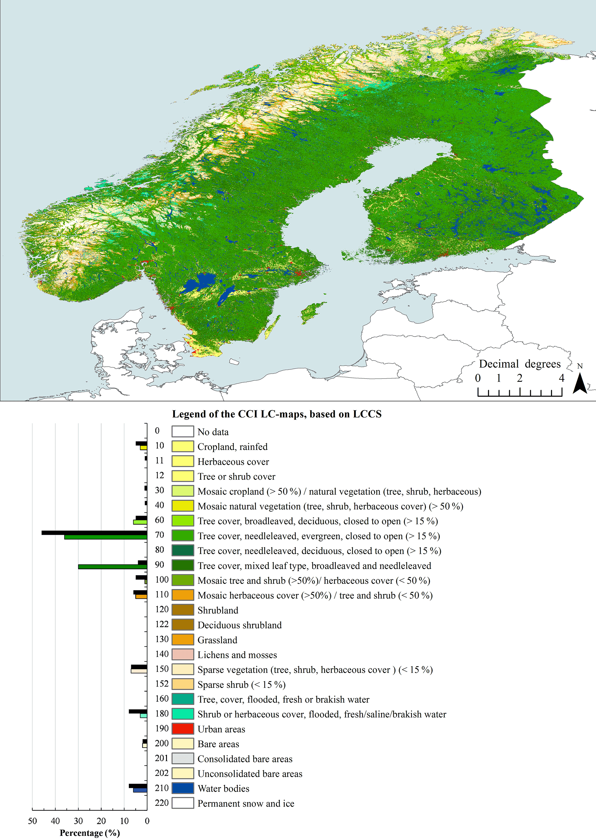
Figure 4Enhanced back-classified map for Fennoscandia. The percentage layers of forest subgroups were used to back-classify the data into ESA LC product classes (see Sect. 2.2.2.). Histograms show LC-class percentages for the enhanced back-classified map (lower bars with colors) and for the ESA LC product (black upper bars). For colors, see the online version of the article.
Table 4Confusion matrix in percentage (%) between the ESA LC product and the enhanced back-classified LC product. Bold font is used to indicate the 10 classes with the highest percentage of pixels. Small percentages are shown as 0.00. The kappa coefficient was 0.55. Label definitions are shown in Fig. 4. In order to compare the two LC products the enhanced LC product was back-classified into ESA LC classes. Column names are the ESA LC-class labels and column sums represent the fraction of that LC class present in the ESA LC product. The row sums represent the fraction of that LC class present in the enhanced back-classified map. The percentage of pixels belonging to the same LC class in both products is shown in diagonal (e.g., the fraction of pixels classified into LC class 70 is 30.3 %). Percentage values outside the diagonal describe the change (“confusion”) between different LC classes (e.g., 14.4 % of pixels classified into LC class 70 by the ESA LC product were classified into LC class 90 in the enhanced back-classified map).
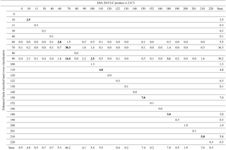

Figure 5Difference in forest extent between the enhanced back-classified map and the ESA LC product. Both types of data were aggregated to ∼ 0.3∘ resolution using mode to display the main differences in the two classifications spatially. The label “Gapfilled forest” is used to indicate areas that were mainly classified as forest by the ESA LC product, but the MS-NFI data indicated non-forest. Other labels (see Fig. 4.) show which main ESA LC classes were classified as forest in the enhanced back-classified map. Note that the confusion matrix between the ESA LC product and enhanced back-classified map was prepared using ∼ 0.003∘ resolution (Table 4), whereas the map resolution shown here is ∼ 0.3∘. For colors, see the online version of the article.
3.3 Forest extent comparison
In order to assess agreement between the two LC products, the enhanced LC product was back-classified into ESA LC classes using the percentage layers of different forest subgroups. The kappa coefficient (measure of agreement that takes into account possible agreement occurring by chance) for classification was 0.55, and the classification accuracy was 0.64 (calculated based on Table 4). The confusion matrix between the ESA LC product and the enhanced back-classified LC map showed that the highest agreement (30.3 %) between the two classification schemes occurred for forest class 70 (i.e., NET; Table 4). The largest fraction of forested pixels in the enhanced back-classified LC map was classified as conifer dominated (36.3 %; Fig. 4). Results showed that 1.5 % of class 70 was classified into class 60 (i.e., BDT), and 14.4 % of ESA LC class 70 was classified as 90 (i.e., “mixed” BDT and NET). The share of mixed forest class (i.e., class 90) was also high (30.2 %). However, the portion of pixels classified as BDT was relatively low (5.5 %). Overall, the enhanced LC product contained 16.4 % more forest classified pixels than the ESA LC product (note: the fraction of gapfilled forest pixels was 4.5 %). Forest area increased by 4.8 % at the expense of the ESA LC class shrub or herbaceous cover (class 180), 4.1 % at the expense of the LC class mosaic tree and shrub (> 50 %; class 100), 2.3 % at the expense of the LC class croplands (class 10), and 1.9 % at the expense of the LC class water bodies (class 210). The classified land area increased by 0.5 % as areas classified as “no data” in the ESA LC product were classified as forest in the enhanced LC product.
The spatial distribution of different LC classes and the class frequencies of the enhanced back-classified map are shown in Fig. 4, which shows both ESA LC-class labels and descriptions (note: ESA LC-product class frequencies are also shown for reference). The difference map of forest cover between the enhanced back-classified LC product and the ESA LC product pointed out that the areal representation of forests differs the most in mountainous areas in Norway and Sweden, south and north Finland, and in middle to south Sweden in the area between Stockholm and lakes Vättern and Vänern (lakes visible in Fig. 4.; Fig. 5.). The areas classified as forest by the ESA LC product but not by MS-NFI data (“gapfilled forest” in Fig. 5.) were mainly located in mountainous areas in Norway and Sweden.
3.4 LAImax map comparison
The enhanced LC product and related LUT produced a Fennoscandic mean LAImax of 3.2. Spatial variations in LAImax appeared more natural when compared to the reference maps (Fig. 6). The standard deviation (SD), a measure of the variability, of LAImax was substantially larger (SD = 2.3) for the enhanced LC product that for the three reference LAImax maps. The smallest mean LAImax values (mean LAImax= 2.4, SD = 0.7) were produced by LAImax values applied in JSBACH. The LAImax map produced using ORCHIDEE had a mean of 3.9 (SD = 0.0 due to applied cross-walking scheme and equal LAImax values for NET and BDT). The largest mean LAImax was produced by LAImax values applied in JULES (mean LAImax= 4.9, SD = 0.9). It is noteworthy that the use of JSBACH and JULES PFT-dependent LAImax values produced unnaturally high LAImax values for the northernmost areas dominated by deciduous species.
This paper is a response to the “call to action” raised in the review by Ellison et al. (2017), which highlighted an urgent need to integrate forest effects on energy balances, hydrology, and climate into policy actions regarding climate change adaptation and mitigation. One of goals of this paper is to foster interdisciplinary discussions on alternative information sources, such as the existing NFI data, to enhance the representation of forest structures in different land modeling frameworks. Although NFIs from different countries have been shaped by local information needs, the work done by the Food and Agriculture Organization (FAO) in conducting global FRAs since 1948 has aided in developing national forest reporting standards. Currently, new assessments are carried out every 5 years and the 2015 assessment covered 93.5 % of the global forest area (Köhl et al., 2015). Thus, as the aim of an FRA is to describe the state and change of the world's forests and keep policy makers informed, the same data could potentially be used to describe the current state of forests in land models. In this study, we developed a simple clustering and classification scheme to allow for the reiteration of our approach to NFI data from other countries. Classifying forests based on the structural properties they share at various successional stages under similar management conditions may be one way to link models of forestry with the land models employed in climate research. Important transient effects could then be included, for example through changes in area under a given successional stage, with forestry models providing the link to the time dimension. Alternatively, distinct rule sets for successional dynamics following management disturbances could be developed analogous to those used to govern growth and competition in dynamic vegetation models (or land models run in dynamic vegetation mode).
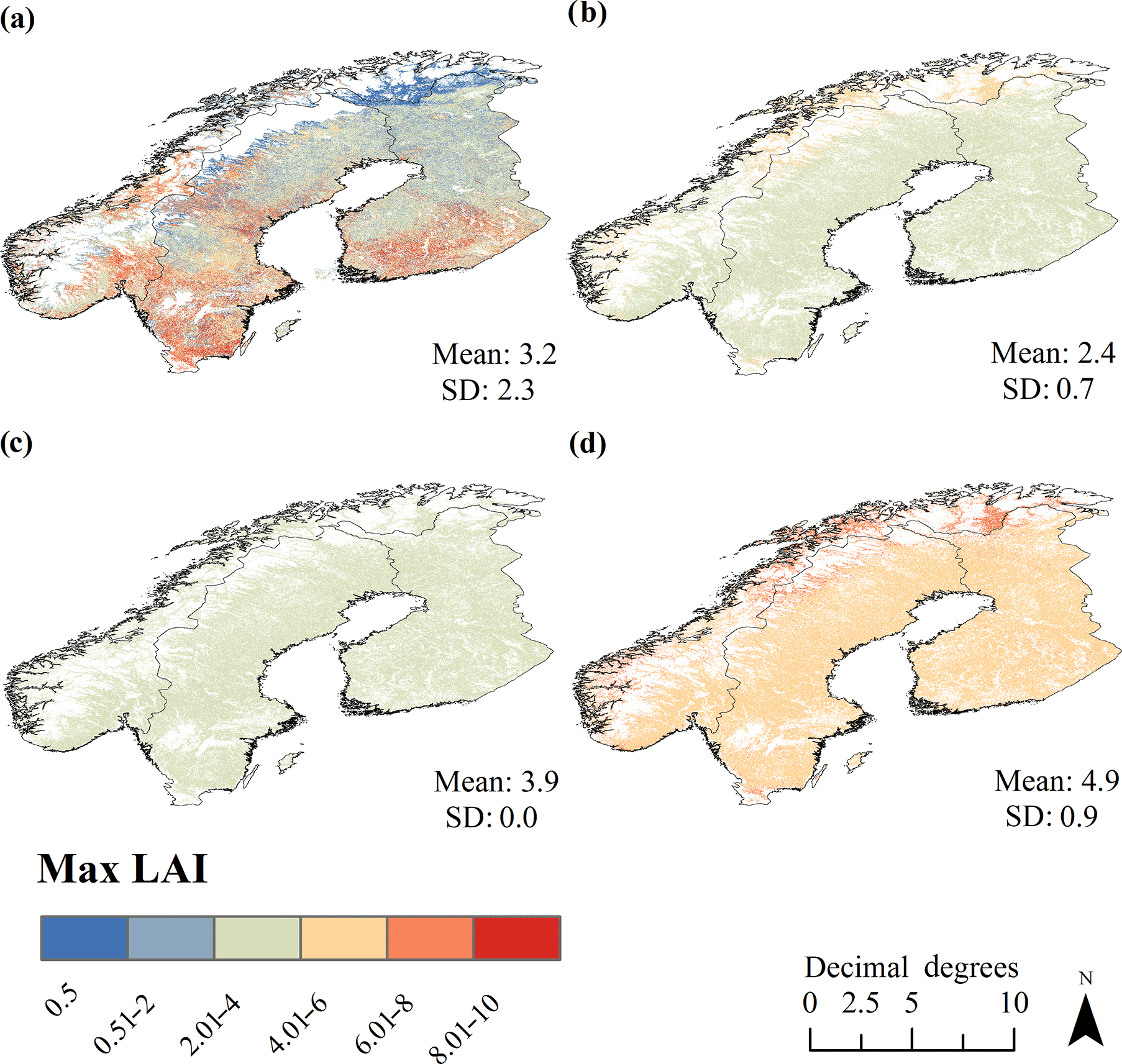
Figure 6Demonstration of how the enhanced LC product and the related LUT may be used to map local variations in important structural attributes in forests, such as maximum growing season LAI (max LAI or LAImax). Maps of LAImax in Fennoscandic forests using (a) our enhanced LC product and the related LUT, (b) ESA LC product and PFT-dependent LAImax values used in JSBACH, (c) ESA LC product and PFT-dependent LAImax values used in ORCHIDEE, and (d) ESA LC product and PFT-dependent LAImax values used in JULES. For colors, see the online version of the article.
Recently, other approaches have been developed for incorporating forest management into existing land surface (climate) models. For example, the radiative-transfer-based land surface model ORCHIDEE was parameterized to simulate the effects of forest management for biogeochemical and biophysical variables (Naudts et al., 2015). The model was parameterized using diameter-at-breast-height (dbh) data from different European NFIs (French, Spanish, Swedish, and German; i.e., the key input values were modeled based on dbh using allometric models), and 12 parameter sets for specific tree species (instead of presenting groups of species such as PFTs) were presented. However, a major drawback of individual tree-based approaches is that existing global LC products are not designated to distinguish between individual species, which limits the spatial domain in which such approaches can be applied. In addition, the need for residual groups remains because individual tree-based approaches are not suited for areas where the forests are essentially mixtures of different tree species. The benefit of defining “broader” PFT classes, such as those developed in this study, is that the broad functional types may be separated from optical satellite data based on differences in optical and structural characteristics of the forests. In the future, as the spectral, spatial, and temporal resolution of optical satellite data improve, the definition of narrower forest classes may be justified. Alternatively, functional traits (FTs) may be used for modeling vegetation–climate interactions (Wullschleger et al., 2014; Verheijen et al., 2013). Commonly, the community-weighted mean trait value (i.e., based on relative abundances of species and their trait values) is used in models that apply the FT concept. While FTs are highly scalable (i.e., from organism to ecosystem scale), well assembled (i.e., leaf, stem, and root traits), and measurable (at least in theory), the downside of FTs is that their applicability is in its infancy, and the lack of standards hinders its practical application. In addition, many traits such as root traits cannot be measured using remote sensing.
At present, some countries, such as Finland and Sweden, have national airborne laser scanning (ALS) campaigns producing high-resolution forest structural data that could be used to obtain more accurate forest height estimates or to develop forest classification schemes for different land models. However, the drawback of these ALS datasets is that they cannot be used to separate different tree species, which is one of the most important forest structural attributes. In addition, as few countries have national ALS datasets, the geographical extent that could be covered using ALS-based forest classification schemes remains limited. At present, the use of optical satellite data to classify forests is unquestionable due to their superior spatial and temporal resolution and will thus probably sustain their role as the most valuable tool for environmental monitoring and mapping. While synthetic aperture radar (SAR) allows for more robust and temporally continuous data collection compared to optical instruments (i.e., SAR is not limited to cloudless conditions unlike optical instruments), the relatively low spatial resolution (km2) cannot be used to separate different aged forests in landscapes that are fragmented (into 0.01 km2 units) by active forest management. Data from SAR could be used to harmonize MS-NFI data from different countries and to provide other land model inputs, such as soil moisture maps. In the future, approaches combining both optical and ALS–SAR data may be expected to become more common and thus allow for the development of more sophisticated forest classification schemes to increase the accuracy of climate predictions.
The forest extent differs significantly between the enhanced LC product and the ESA LC product because they employ different forest definitions. The ESA LC product is based on series of satellite surface reflectance data (i.e., between years 1992 and 2015) and the LC class is deduced based on pixel reflectance properties. However, processing the MS-NFI data employs a forest mask that delineates potential forest areas prior to the kNN estimation (i.e., clear-cuts and harvest are seen as a natural part of forest development, and thus pixels inside the forest mask may have V= 0 or H= 0; Supplement S4). For example, it is not clear if a sapling stand with V= 3 (m3 ha−1) and H= 3 (m) would classify as forest based only on its reflectance. Thus, the enhanced LC product cannot be directly used to validate the ESA LC product. In addition, differences in forest extent are propagated by the different spatial resolutions of the input reflectance data (i.e., the probability of having “mixed” class pixels is higher using lower-resolution data) and data aggregation using the mode (i.e., the most abundant classes will become more common). The influence of spatial resolution of the input data and the applied data aggregation method may be observed, for example, around water bodies in Finland and in Sweden (e.g., Figs. 4 and 5). For example, a single ESA LC pixel (∼ 90 000 m2) classified as water (located next to a larger water body) may contain more pixels classified as forest than water in high-resolution (< 900 m2) MS-NFI data (e.g., Huang et al., 2002) and thus be classified as forest if data are aggregated using mode. The forest area of the enhanced LC product is also larger than in the ESA LC product because MS-NFI data were complemented with the ESA LC-product data, and pixels that were classified as forest by the ESA LC product but did not contain forest according to the MS-NFI data were gapfilled.
The presented forest classification scheme has many levels to serve the needs of different users (Supplement S5). For example, for climate and hydrological modeling requiring full spatial coverage, the gapfilled pixels and non-forest LC classes are provided. Researchers that are able to run their models with no data may select to remove the gapfilled pixels prior to analysis. Remote sensing scientists may wish to use only “true” forest pixels and extract areas belonging to different species groups or subgroups or select areas where the fraction of forests is lower or higher (i.e., “open” or “closed” following ESA LC-product legend definitions). In addition, the percentage layers – or the relative abundance of different forest subgroups within each LC pixel in MS-NFI data – provide land modelers with more control and flexibility in terms of the number of input LC classes in different land models. The percentage layers for different forest subgroups may be used to obtain complete LC distributions for Fennoscandia, or alternatively, a modeler may choose, for example, to use three of the most abundant forest classes instead of holding onto the most abundant forest class. The percentage layers also provide more flexibility for cross-walking (Poulter et al., 2015) across different spatial resolutions. Our forest classification scheme and the related map products (i.e., enhanced LC product and the percentage layers) allow for customized model “inputs” to fit the needs (or requirements) of various land models.
The development of cross-walking tables has previously been complicated by the fact that the number and definition of PFTs used in today's land models vary along with the limited availability of spatially and temporally representative input LC datasets (Poulter et al., 2015). The presented forest classification scheme (Majasalmi et al., 2017) has many levels to serve the needs of different users (Supplement S5). The new ESA LC-product series was the first to overcome the aforementioned challenges and demonstrate how to compile an LC-product series that optimally serves the needs of various users. Our work in this paper does not imply that the ESA LC product and cross-walking scheme (or the model- and PFT-dependent parameter values) are necessarily wrong per se, but simply presents an alternative approach to classification that explicitly accounts for the structural variation in managed forests in different successional stages. The flexibility in the spatial resampling of the ESA LC product is preserved by our approach (i.e., the idea of our “percentage layers” correspond with the “fractional area” contribution employed by the ESA LC product; Poulter et al., 2015), thus respecting the efforts of ESA LC-product developers. Our LUT demonstration showed that by using the enhanced LC product with its related LUT, the description of LAImax appeared more natural compared to the LAImax maps of JULES, ORCHIDEE, and JSBACH compiled using the ESA LC-product classification, PFT cross-walking table (Poulter et al., 2015), and model- and PFT-dependent LAImax values. While the accuracy of our product cannot generally be determined, it presents a new approach to quantify the present state of the key forest structural attributes of managed forests in Fennoscandia. In regional modeling studies, based on our results, it appears worth the effort to use the enhanced LC product instead of the original ESA LC product when cross-walking from LC classes to PFTs to obtain more truthful initial values of the key structural variables (i.e., LAImax, zbottom, ztop). The enhanced LC product may be used for forecasting and back-casting the impacts of forest management on energy, water, and carbon cycling; whether our enhanced forest classification leads to improved regional climate predictions linked to transient changes occurring in forests over time remains the subject of future research activity.
To our knowledge, this is the first study to use NFI data together with MS-NFI maps to enhance the characterization of forest structure in a format that is compatible with many land surface (climate) models (i.e., in modeling frameworks) in which changes in vegetation structure are captured by area-based changes in LC (or PFT). The methods used for creating the LUT were carefully explained to allow other researchers to replicate the same procedures using NFI data from other countries. The benefit of the classification scheme described in this study is that the required data (i.e., NFI data and MS-NFI maps of species, V, and H) are readily available for many countries. Future research is needed to develop recommendations and guidelines for prescribing future forest transitions under changing climate and management regimes in different land models and modeling frameworks.
The MS-NFI forest resource maps for Finland are available through the Natural Resources Institute Finland (LUKE) portal: http://kartta.luke.fi/opendata/valinta.html. For Sweden the forest maps may be obtained through the Swedish University of Agricultural Sciences (SLU) portal: http://www.slu.se/en/Collaborative-Centres-and-Projects/the-swedish-national-forest-inventory/forest-statistics/slu-forest-map/. For Norway the MS-NFI data are available by request from the Norwegian Institute of Bioeconomy Research (NIBIO). The enhanced LC product for Fennoscandia, including the percentage layers, can be downloaded from https://doi.org/10.21350/7zZEy5w3T (Majasalmi et al., 2017).
The supplement related to this article is available online at: https://doi.org/10.5194/bg-15-399-2018-supplement.
The authors declare that they have no conflict of interest.
The research was funded by the Research Council of Norway, grant number
250113/F20. We acknowledge the work done by the ESA CCI Land Cover project
and the
constructive feedback from three anonymous reviewers.
Edited by: Kirsten Thonicke
Reviewed by: three anonymous referees
Ahlstrøm, A. P., Bjørkelo, K., and Frydenlund, J.: AR5 KLASSIFIKASJONSSYSTEM: Klassifikasjon av arealressurser. Rapport fra Skog og landskap 06/14: III, 38s, http://www.skogoglandskap.no/filearchive/rapport_06-2014.pdf (last access: 13 January 2018), 2014.
Bivand, R., Keitt, T., and Rowlingson, B.: Bindings for the 'Geospatial' Data Abstraction Library, https://cran.r-project.org/web/packages/rgdal/rgdal.pdf (last access: 13 January 2018), 2017.
Bonan, G. B.: Forests and climate change: forcings, feedbacks, and the climate benefits of forests, Science, 320, 1444–1449, 2008.
Bonan, G.: Ecological Climatology: Concepts and Applications, Cambridge University Press, Cambridge, https://doi.org/10.1017/CBO9781107339200, 2015.
Bright, R. M., Antón-Fernández, C., Astrup, R., Cherubini, F., Kvalevåg, M. M., and Strømman, A. H.: Climate change implications of shifting forest management strategy in a boreal forest ecosystem of Norway, Glob. Change Biol., 20, 607–621, 2014.
Clark, D. B., Mercado, L. M., Sitch, S., Jones, C. D., Gedney, N., Best, M. J., Pryor, M., Rooney, G. G., Essery, R. L. H., Blyth, E., Boucher, O., Harding, R. J., Huntingford, C., and Cox, P. M.: The Joint UK Land Environment Simulator (JULES), model description – Part 2: Carbon fluxes and vegetation dynamics, Geosci. Model Dev., 4, 701–722, https://doi.org/10.5194/gmd-4-701-2011, 2011.
ESA LC: European Space Agency (ESA) Climate Change Initiative (CCI) Land Cover (LC)-product (v.2.0.7), https://www.esa-landcover-cci.org/?q=node/175, Manual: CCI-LC-PUGV2. last access: 10 October 2017.
Chen, J. M. and Black, T. A.: Defining leaf area index for non-flat leaves, Plant Cell Environ., 15, 421–429, 1992.
Ellison, D., Morris, C. E., Locatelli, B., Sheil, D., Cohen, J., Murdiyarso, D., Gutierrez, V., Van Noordwijk, M., Creed, I. F., Pokorny, J., and Gaveau, D.: Trees, forests and water: Cool insights for a hot world, Global Environ. Chang., 43, 51–61, 2017.
FAO, Food and Agriculture Organization of the United Nations: Global forest resources assessment, http://www.fao.org/3/a-i4808e.pdf, 253 pp., 2015.
Friedl, M. A., McIver, D. K., Hodges, J. C., Zhang, X. Y., Muchoney, D., Strahler, A. H., Woodcock, C. E., Gopal, S., Schneider, A., Cooper, A., and Baccini, A.: Global land cover mapping from MODIS: algorithms and early results, Remote Sens. Environ., 83, 287–302, 2002.
Fridman, J., Holm, S., Nilsson, M., Nilsson, P., Ringvall, A. H., and Ståhl, G.: Adapting National Forest Inventories to changing requirements – the case of the Swedish National Forest Inventory at the turn of the 20th century, Silva Fenn., 48, 1–29, 2014.
Gjertsen, A. K.: Accuracy of forest mapping based on Landsat TM data and a kNN-based method, Remote Sens. Environ., 110, 420–430, 2007.
Gjertsen, A. K.: SAT-SKOG kom på Internett i 2009, Årsmelding fra Skog og landskap 2009: 27, http://www.skogoglandskap.no/filearchive/sat_skog_kom_pa_ internett_i_2009.pdf (last access: 13 January 2018), 2009.
GCOS, Global Climate Observing System: Essential Climate Variables, http://www.wmo.int/pages/prog/gcos/index.php?name=EssentialClimateVariables (last access: 13 January 2018), 2012.
Hansen, M. C., DeFries, R. S., Townshend, J. R., and Sohlberg, R.: Global land cover classification at 1 km spatial resolution using a classification tree approach, Int. J. Remote Sens., 21, 1331–1364, 2000.
Hijmans, R. J.: Geographic Data Analysis and Modeling, https://cran.r-project.org/web/packages/raster/raster.pdf (last access: 13 January 2018, 2017.
Huang, C., Townshend, J. R., Liang, S., Kalluri, S. N., and DeFries, R. S.: Impact of sensor's point spread function on land cover characterization: assessment and deconvolution, Remote Sens. Environ., 80, 203–212, 2002.
Kassambara, A. and Mundt, F.: Extract and Visualize the Results of Multivariate Data Analyses, version 1.0.5, https://cran.r-project.org/web/packages/factoextra/factoextra.pdf (last access: 13 January 2018), 2017.
Kaufman, L. and Rousseeuw, P. J.: Finding Groups in Data: An Introduction to Cluster Analysis, Wiley, New York, 1990.
Ketchen Jr., D. J. and Shook, C. L.: The application of cluster analysis in strategic management research: an analysis and critique, Strateg. Manage. J., 441–458, 1996.
Köhl, M., Lasco, R., Cifuentes, M., Jonsson, Ö., Korhonen, K. T., Mundhenk, P., de Jesus Navar, J., and Stinson, G.: Changes in forest production, biomass and carbon: Results from the 2015 UN FAO Global Forest Resource Assessment, Forest Ecol. Manag., 352, 21–34, 2015.
Kuhn, M.: Building Predictive Models in R Using the caret Package, J. Stat. Softw., 28, http://download.nextag.com/cran/web/packages/caret/caret.pdf (last access: 13 January 2018), 2008.
Kuuluvainen, T., Tahvonen, O., and Aakala, T.: Even-aged and uneven-aged forest management in boreal Fennoscandia: a review, Ambio, 41, 720–737, 2012.
Lathière, J., Hauglustaine, D. A., Friend, A. D., De Noblet-Ducoudré, N., Viovy, N., and Folberth, G. A.: Impact of climate variability and land use changes on global biogenic volatile organic compound emissions, Atmos. Chem. Phys., 6, 2129–2146, https://doi.org/10.5194/acp-6-2129-2006, 2006.
Lawrence, P. J. and Chase, T. N.: Representing a new MODIS consistent land surface in the Community Land Model (CLM 3.0), J. Geophys. Res.-Biogeo., 112, G01023, https://doi.org/10.1029/2006JG000168, 2007.
Lawrence, P. J., Feddema, J. J., Bonan, G. B., Meehl, G. A., O'Neill, B. C., Oleson, K. W., Levis, S., Lawrence, D. M., Kluzek, E., Lindsay, K., and Thornton, P. E.: Simulating the biogeochemical and biogeophysical impacts of transient land cover change and wood harvest in the Community Climate System Model (CCSM4) from 1850 to 2100, J. Climate, 25, 3071–3095, 2012.
LUKE: Natural Resources Institute Finland, Forest resource maps, http://kartta.luke.fi/opendata/valinta.html, last access: 15 October 2016.
Mahalanobis, P. C.: On the generalized distance in statistics, Proceedings of The National Institute of Sciences of India, 12, 49–55, 1936.
Maechler, M.: “Finding Groups in Data”: Cluster Analysis Extended Rousseeuw et al., https://cran.r-project.org/web/packages/cluster/cluster.pdf (last access: 13 January), 2017.
Majasalmi, T., Eisner, S., Astrup, R., Fridman, J., and Bright, R. M.: Enhanced LC-product for Fennoscandia, https://doi.org/10.21350/7zZEy5w3, 2017.
Nakai, T., Sumida, A., Kodama, Y., Hara, T., and Ohta, T.: A comparison between various definitions of forest stand height and aerodynamic canopy height, Agr. Forest Meteorol., 150, 1225–1233, 2010.
Naudts, K., Ryder, J., McGrath, M. J., Otto, J., Chen, Y., Valade, A., Bellasen, V., Berhongaray, G., Bönisch, G., Campioli, M., Ghattas, J., De Groote, T., Haverd, V., Kattge, J., MacBean, N., Maignan, F., Merilä, P., Penuelas, J., Peylin, P., Pinty, B., Pretzsch, H., Schulze, E. D., Solyga, D., Vuichard, N., Yan, Y., and Luyssaert, S.: A vertically discretised canopy description for ORCHIDEE (SVN r2290) and the modifications to the energy, water and carbon fluxes, Geosci. Model Dev., 8, 2035–2065, https://doi.org/10.5194/gmd-8-2035-2015, 2015.
Naudts, K., Chen, Y., McGrath, M. J., Ryder, J., Valade, A., Otto, J., and Luyssaert, S. Europe's forest management did not mitigate climate warming, Science, 351, 597–600, 2016.
Newton, P. F.: Stand density management diagrams: review of their development and utility in stand-level management planning, Forest Ecol. Manag., 98, 251–265, 1997.
Oke, T. R.: Boundary layer climates, 2nd Edn., Routledge, 2002.
Oleson, K. W., Lawrence, D. M., Bonan, G. B., Drewniak, B., Huang, M., Koven, C. D., Lewis, S., Li, F., Riley, W. J., Subin, Z. M., Swenson, S. C., Thornton, P. E., Bozbiyik, A., Fisher, R., Heald, C. L., Kluzek, E., Lamarque, J.-F., Lawrence, P. J., Leung, L. R., Lipscomb, W., Muszala, S., Ricciuto, D. M., Sacks, W., Sun, Y., Tang, J., and Yang, Z.-L.: Technical description of version 4.5 of the Community Land Model (CLM), NCAR Technical Note NCAR/TN-503+STR, The National Center for Atmospheric Research (NCAR), Boulder, CO, USA, 420 pp., 2013.
Poulter, B., MacBean, N., Hartley, A., Khlystova, I., Arino, O., Betts, R., Bontemps, S., Boettcher, M., Brockmann, C., Defourny, P., Hagemann, S., Herold, M., Kirches, G., Lamarche, C., Lederer, D., Ottlé, C., Peters, M., and Peylin, P.: Plant functional type classification for earth system models: results from the European Space Agency's Land Cover Climate Change Initiative, Geosci. Model Dev., 8, 2315–2328, https://doi.org/10.5194/gmd-8-2315-2015, 2015.
Reick, C., Gayler, V., Raddatz, T., Schnur, R., and Wilkenskjeld, S.: JSBACH – The new land component of ECHAM, Max Planck Institute for Meteorology, 20146 Hamburg, Germany, 2012.
Reick, C. H., Raddatz, T., Brovkin, V., and Gayler, V.: Representation of natural and anthropogenic land cover change in MPI-ESM, J. Adv. Model Earth Sy., 5, 459–482, 2013.
Schürmann, G. J., Kaminski, T., Köstler, C., Carvalhais, N., Voßbeck, M., Kattge, J., Giering, R., Rödenbeck, C., Heimann, M., and Zaehle, S.: Constraining a land-surface model with multiple observations by application of the MPI-Carbon Cycle Data Assimilation System V1.0, Geosci. Model Dev., 9, 2999–3026, https://doi.org/10.5194/gmd-9-2999-2016, 2016.
SLU, Swedish University of Agricultural Sciences Forest maps, http://www.slu.se/en/Collaborative-Centres-and-Projects/the-swedish-national-forest-inventory/forest-statistics/slu-forest-map/, last access: 29 October 2016.
Tomppo, E., Katila, M., Mäkisara, K., and Peräsaari, J.: The Multi-source National Forest Inventory of Finland – methods and results 2011. Metlan työraportteja/Working Papers of the Finnish Forest Research Institute 319, 224 pp., http://www.metla.fi/julkaisut/workingpapers/2014/mwp319.htm (last access: 13 January 2018), 2014.
Tomter, S., Hylen, G., and Nilsen, J.-E.: Norways national forest inventory, in: National forest inventories: pathways for common reporting, edited by: Tomppo, E., Gschwantner, T., Lawrence, M., and McRoberts, R. E., Springer, Berlin, 2010.
Verheijen, L. M., Brovkin, V., Aerts, R., Bönisch, G., Cornelissen, J. H. C., Kattge, J., Reich, P. B., Wright, I. J., and van Bodegom, P. M.: Impacts of trait variation through observed trait-climate relationships on performance of an Earth system model: a conceptual analysis, Biogeosciences, 10, 5497–5515, https://doi.org/10.5194/bg-10-5497-2013, 2013.
Wullschleger, S. D., Epstein, H. E., Box, E. O., Euskirchen, E. S., Goswami, S., Iversen, C. M., Kattge, J., Norby, R. J., van Bodegom, P. M., and Xu, X.: Plant functional types in Earth system models: past experiences and future directions for application of dynamic vegetation models in high-latitude ecosystems, Ann. Bot., 114, 1–16, https://doi.org/10.1093/aob/mcu077, 2014.