the Creative Commons Attribution 4.0 License.
the Creative Commons Attribution 4.0 License.
 | 10 Apr 2019
Simulating the atmospheric CO2 concentration across the heterogeneous landscape of Denmark using a coupled atmosphere–biosphere mesoscale model system
Anne Sofie Lansø
Thomas Luke Smallman
Jesper Heile Christensen
Mathew Williams
Kim Pilegaard
Lise-Lotte Sørensen
Camilla Geels
Although coastal regions only amount to 7 % of the global oceans, their contribution to the global oceanic air–sea CO2 exchange is proportionally larger, with fluxes in some estuaries being similar in magnitude to terrestrial surface fluxes of CO2.
Across a heterogeneous surface consisting of a coastal marginal sea with estuarine properties and varied land mosaics, the surface fluxes of CO2 from both marine areas and terrestrial surfaces were investigated in this study together with their impact in atmospheric CO2 concentrations by the usage of a high-resolution modelling framework. The simulated terrestrial fluxes across the study region of Denmark experienced an east–west gradient corresponding to the distribution of the land cover classification, their biological activity and the urbanised areas. Annually, the Danish terrestrial surface had an uptake of approximately −7000 GgC yr−1. While the marine fluxes from the North Sea and the Danish inner waters were smaller annually, with about −1800 and 1300 GgC yr−1, their sizes are comparable to annual terrestrial fluxes from individual land cover classifications in the study region and hence are not negligible. The contribution of terrestrial surfaces fluxes was easily detectable in both simulated and measured concentrations of atmospheric CO2 at the only tall tower site in the study region. Although, the tower is positioned next to Roskilde Fjord, the local marine impact was not distinguishable in the simulated concentrations. But the regional impact from the Danish inner waters and the Baltic Sea increased the atmospheric concentration by up to 0.5 ppm during the winter months.
- Article
(5952 KB) - Full-text XML
-
Supplement
(12424 KB) - BibTeX
- EndNote


Understanding the natural processes responsible for absorbing just over half of the anthropogenic carbon emitted to the atmosphere will help decipher future climatic pathways. During the last decade, the ocean and the biosphere are estimated to take up to 2.4±0.5 and 3.0±0.8 PgC yr−1 of the 9.4±0.5 PgC yr−1 of anthropogenic carbon emitted to the atmosphere (Le Quéré et al., 2018). The heterogeneity and the dynamics of the surface complicates such estimates.
Biosphere models of various complexity have been developed to spatially simulate surface fluxes of CO2, but future estimates of the land uptake are bound with large uncertainties (Friedlingstein et al., 2014) that can be attributed to model structural uncertainties, uncertain observations and lack of model benchmarking (Cox et al., 2013; Luo et al., 2012; Lovenduski and Bonan, 2017). To have the best chance of accurately predicting the future evolution of the carbon cycle, and its implications for our climate, it is important to minimise the uncertainties that exist presently (Carslaw et al., 2018). Enhanced knowledge and a better process understanding in ecological theory and modelling could potentially reduce the model structural uncertainties (Lovenduski and Bonan, 2017), which together with improvements in spatial surface representation could minimise the current uncertainties.
Studying surface exchanges of CO2 on regional to local scale can be accomplished with mesoscale atmospheric transport models. Their resolution is in the range from 2 to 20 km, and their advantage is their capability to get a better process understanding of both atmospheric and surface exchange mechanisms in order to improve the link between observations and models at all scales, i.e. for both mesoscale, regional and global models (Ahmadov et al., 2007). The higher spatial resolution of mesoscale models allows for a better representation of atmospheric flows and for a more detailed surface description, which is necessary in particular for heterogeneous areas. In previous mesoscale model studies, biosphere models have been coupled to the mesoscale atmospheric models ranging in their complexity, from a simple diagnostic (Sarrat et al., 2007b; Ahmadov et al., 2007, 2009) to mechanistic-process-based biosphere models (Tolk et al., 2009; Ter Maat et al., 2010; Smallman et al., 2014; Uebel et al., 2017). The modelled CO2 concentrations and surface fluxes from mesoscale model systems compare better with observations than global model systems (Ahmadov et al., 2009). The atmospheric impact on surface processes related to the ecosystem's sensitivity and CO2 exchange can be examined in greater detail (Tolk et al., 2009), and tall tower footprints can be studied more concisely (Smallman et al., 2014).
Heterogeneity can also be considerable in coastal oceans, and like terrestrial surface fluxes, the high spatio-temporal variability leads to large uncertainties in estimates of coastal air–sea CO2 fluxes (Cai, 2011; Laruelle et al., 2013). Coastal seas play an important role in the carbon cycle facilitating lateral transport of carbon from land to open oceans, but almost 20 % of the carbon entering estuaries is released into the atmosphere, while 17 % of the carbon inputs to coastal shelves come from atmospheric exchange (Regnier et al., 2013). The air–sea CO2 exchange is in general numerically larger for estuaries than shelf seas (Chen et al., 2013; Laruelle et al., 2010, 2014) and can, for estuaries, be as large as 1958 gC m−2 yr−1, while continental shelf seas have fluxes in the range of −154 to 180 gC m−2 yr−1 (Chen et al., 2013). The large spatial and temporal heterogeneity of the coastal ocean adds to the large uncertainty related to the annual estimates of the air–sea CO2 exchange (Regnier et al., 2013). The observed high spatial and temporal variability (Kuss et al., 2006; Leinweber et al., 2009; Vandemark et al., 2011; Norman et al., 2013; Mørk et al., 2016) are not always included in marine models (Omstedt et al., 2009; Gypens et al., 2011; Kuznetsov and Neumann, 2013; Gustafsson et al., 2015; Valsala and Murtugudde, 2015), let alone being taken into account in atmospheric mesoscale systems simulating CO2 (Sarrat et al., 2007a; Geels et al., 2007; Law et al., 2008; Tolk et al., 2009; Broquet et al., 2011; Kretschmer et al., 2014). But a recent study found that short-term variability in the partial pressure of surface water CO2 (pCO2) can substantially affect simulated annual fluxes in certain coastal areas – in their case the Baltic Sea (Lansø et al., 2017). Moreover, direct eddy covariance (EC) measurements in the Baltic Sea have shown that upwelling events with rapid changes in pCO2 greatly increase the air–sea CO2 exchange (Kuss et al., 2006; Rutgersson et al., 2009; Norman et al., 2013).
In this study we aim to simulate surface exchanges of CO2 at a high spatio-temporal resolution across a region neighbouring the Baltic Sea, alternating between land and coastal sea together with mesoscale atmospheric transport. A newly developed mesoscale modelling system is used to assess and understand the dynamics and relative importance of the marine and terrestrial CO2 fluxes. The Danish Eulerian Hemispheric Model (DEHM) forms the basis of the framework, while the mechanistic biospheric soil–plant–atmosphere model (SPA) is dynamically coupled to the atmospheric model. Both models are driven by methodological data from the Weather Research and Forecasting model (WRF). The air–sea CO2 exchange is simulated at a high temporal resolution with the best applicable surface fields of pCO2 for the Danish marine areas. Tall tower observations are used to evaluate the simulated atmospheric concentrations of CO2.
Section 2 is dedicated to describing the study region, which is followed by a detailed description and evaluation of the atmospheric and biospheric model components of the developed model system in Sect. 3. Section 4 contains results, while the Discussion and Conclusions follow in Sects. 5 and 6.
The study area is comprised of Denmark, a country that is characterised by a mainland (Jutland) and many smaller islands, all containing a varied land mosaic of urban, forest and agricultural areas. With more than 7300 km of coastline encircling approximately 43 000 km2 of land, many land–sea borders are found throughout the country, adding to the complexity (Fig. 1). Denmark is positioned in the transition zone between the Baltic Sea, a marginal coastal sea with low salinity, and the North Sea, a continental shelf sea. Bordering the Baltic Sea, the Danish inner waters are rich in nutrients and organic material (Kuliński and Pempkowiak, 2011). This fosters high biological activity in spring and summer, lowering surface water pCO2 and allowing for uptake of atmospheric CO2. In winter, mineralisation increases pCO2 (Wesslander et al., 2010), and outgassing of CO2 to the atmosphere takes place. The North Sea is a persistent sink of atmospheric CO2, where a continental shelf-sea pump efficiently removes pCO2 from the surface water and transports it to the North Atlantic Ocean (Thomas et al., 2004). This study uses the definition of the Danish exclusive economic zone (EEZ) to estimate the Danish air–sea CO2 exchange, as the coastal state (in this case Denmark) has the right to explore, exploit and manage all resources found within its EEZ (United Nations Chapter XXI, 1984). The Danish EEZ is approximately 105 000 km2.
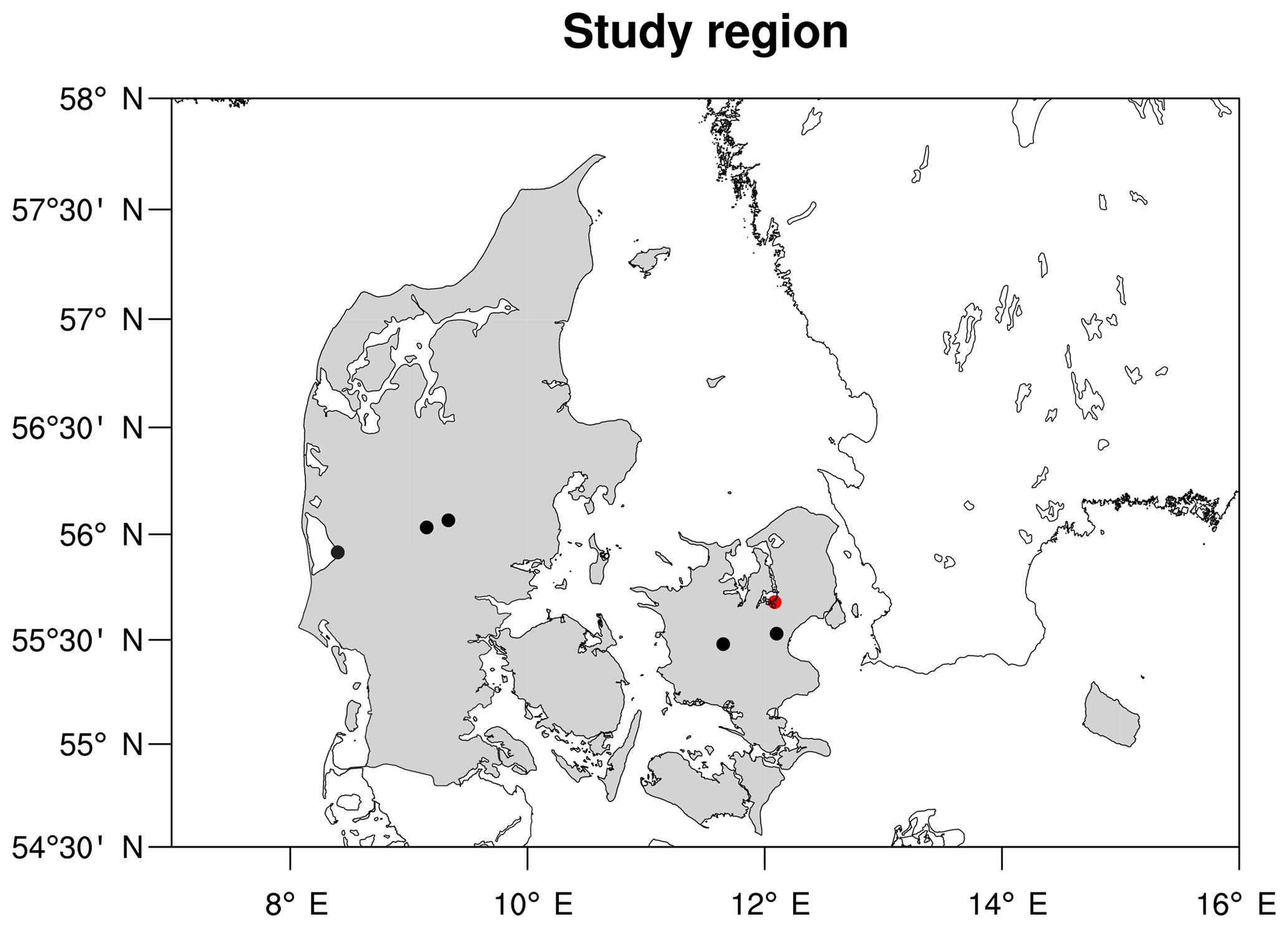
Figure 1The study region of Denmark (land masses in grey), with the location of the five EC sites shown in black and the Risø campus tall tower site indicated in red.
A tiling approach with the seven most common biospheric land cover classifications were selected for the current study, including deciduous forest (3348 km2), evergreen forest (1870 km2), winter barley (1211 km2), winter wheat and other winter crops (9269 km2), spring barley and other spring crops (5368 km2), grassland (6924 km2), and agricultural other (3909 km2), but excluding urbanised areas. The agricultural other land cover classification includes all agriculture that does not classify as cereals, and as such contains root crops, fruits, corn, hedgerows and “undefined” agriculture. This classification corresponds to the actual crop distribution of 2011 (Jepsen and Levin, 2013).
2.1 Observations of atmospheric CO2
One tall tower is found within the study area on the eastern inner shore of Roskilde Fjord. Here atmospheric continuous measurements have been conducted at the Risø campus tower site (55∘42′ N, 12∘05′ E) during 2013 and 2014. The tower is located on small hill 6.5 m above sea level (Sogachev and Dellwik, 2017). Roskilde Fjord is a narrow micro-tidal estuary that is 40 km long with a surface area of 123 km2, has a mean depth of 3 m and is found in the sector 200–360∘ relative to the Risø campus tower (Mørk et al., 2016). The city of Roskilde, with around 50 000 inhabitants, is positioned approximately 5 km to the southwest of the site, while Copenhagen lies 20 km to the east.
The tall tower continuous measurements of atmospheric CO2 concentrations at the Risø campus tower were carried out by the use of a Picarro G1301 placed in a heated building. The inlet was 118 m above the surface, and the tube flow rate was 5 slpm. The Picarro was new and calibrated by the factory. The calibration was checked by a standard gas of 1000 ppm CO2 in atmospheric air (Air Liquide). During the measurement period from the middle of 2013 to the end of 2014, the instrument showed no other drift than the general increase in the global atmospheric concentration.
The model framework used in the present study consists of two models: DEHM and SPA. A coupling between the two was made for the innermost nest of DEHM in order to simulate the exchange of CO2 between the atmosphere and terrestrial biosphere at a high temporal (1 h) and spatial resolution (5.6 km × 5.6 km) for the area of Denmark.
3.1 DEHM
DEHM is an atmospheric chemical transport model covering the Northern Hemisphere, with a polar stereographic projection true at 60∘ N. Originally developed to study sulfur and sulfate (Christensen, 1997), the DEHM model now contains 58 chemical species and nine groups of particular matter (Brandt et al., 2012). This adaptable model has been used to study atmospheric mercury (Christensen et al., 2004), persistent organic pollutants (Hansen et al., 2004), biogenic volatile organic compounds' influence on air quality (Zare et al., 2014), emission and transport of pollen (Skjøth et al., 2007), ammonia and nitrogen deposition (Geels et al., 2012a, b), and atmospheric CO2 (Geels et al., 2002, 2004, 2007; Lansø et al., 2015). The CO2 version of DEHM was used in the present study. DEHM has 29 vertical levels distributed from the surface to the 100 hPa surface with approximately 10 levels in the boundary layer. Horizontally, DEHM has 96 × 96 grid points, which through its nesting capabilities increase in resolution from 150 km × 150 km in the main domain to 50 km × 50 km, 16.7 km × 16.7 km and 5.6 km × 5.6 km in the three nests. The two-way nesting replaces the concentrations in the coarser grids by the values from the finer grids.
3.1.1 Surface fluxes in DEHM
Anthropogenic emissions of CO2, wildfire emissions and optimised biospheric fluxes from the NOAA ESRL CarbonTracker system (Peters et al., 2007) version CT2015 were used as inputs to DEHM. Their resolution is 1∘ × 1∘, with updated values every third hour. Similarly, CT2015 3-hourly mole fractions of CO2 were read in as boundary conditions at the lateral boundaries of the main domain.
Hourly anthropogenic emissions on a 10 km × 10 km grid from the Institute of Energy Economics and Rational Energy Use (IER, Pregger et al., 2007) were applied for Europe instead of emissions from CT2015. Furthermore, these are, for the area of Denmark, substituted by hourly anthropogenic emissions with an even higher spatial resolution of 1 km × 1 km (Plejdrup and Gyldenkærne, 2011). As the European and Danish emission inventories were from 2005 and 2011, respectively, the emissions were scaled to annual national total CO2 emissions of fossil fuel and cement production conducted by EDGAR (Olivier et al., 2014) in order to include the yearly variability in national anthropogenic CO2 emissions.
3.1.2 Air–sea CO2 exchange
The exchange of CO2 between the atmosphere and the ocean, , was calculated by , where K is solubility of CO2 calculated as in Weiss (1974), k660 is the transfer velocity of CO2 normalised to a Schmidt number of 660 at 20 ∘C, and ΔpCO2 is the difference in partial pressure of CO2 between the surface water and the overlying atmosphere. The transfer velocity parameterisation , where is the wind speed at 10 m, determined by Ho et al. (2006), has been found to match Danish fjord systems (Mørk et al., 2016) and was applied in the current study. Surface values of marine pCO2 were described by a combination of the open-ocean surface water climatology of pCO2 by Takahashi et al. (2014) and the climatology developed by Lansø et al. (2015, 2017) for the Baltic Sea and Danish waters. Furthermore, short-term temporal variability was accounted for in the surface water pCO2 by imposing monthly mean diurnal cycles onto the monthly climatologies following the method described in Lansø et al. (2017).
3.1.3 Meteorological drivers
The necessary meteorological parameters for DEHM were simulated by the WRF (Skamarock et al., 2008), nudged by 6-hourly ERA-Interim meteorology (Dee et al., 2011) for the period 2008 to 2014, and were also used as initial and boundary conditions. In WRF the Noah land surface model, the Eta similarity surface layer and the Mellor–Yamada–Janjic boundary layer scheme were chosen to simulate surface and boundary layer dynamics. The CAM scheme was used for long- and short-wave radiation, the WRF single-moment five-class microphysics scheme was applied for microphysical processes, and the Kain–Fritsch scheme was used for cumulus parameterisation (Skamarock et al., 2008). In WRF the same nests were chosen as in DEHM, and the meteorological outputs were saved every hour. To get the sub-hourly values that match the time step in DEHM, a temporal interpolation was conducted between the hourly time steps when DEHM was reading the hourly meteorological data. Furthermore, a correction of the horizontal wind speed was conducted in DEHM to ensure mass conservation and compliance with surface pressure (Bregman et al., 2003).
3.1.4 Evaluation of meteorological drivers
We did not have access to measurements from official meteorological observational sites. Thus, for the evaluation of the meteorological drivers, measurements from different types of monitoring sites were used, comprised of three air pollution monitoring sites, three FLUXNET sites, and three sites from the Danish Hydrological Observatory (HOBE; Table 1).
Wind directions, investigated by comparing wind roses made from WRF outputs and measurements, were at most sites reasonably captured by WRF (see Figs. S1–S3 in the Supplement). At several sites the frequency of wind directions from the west were overestimated by WRF, mainly at the expense of southern winds. However, the opposite was the case at Aarhus, where the effect of street canyons was likely causing higher occurrences from due west in the observed wind directions. The wind velocities were in general overestimated by WRF with an average of 1.1 m s−1, with the greatest differences at the same sites experiencing most problems in reproducing the observed wind direction patterns (Fig. 2). Moreover, at the Risø campus tower site the wind velocities were underestimated.
Table 1Location of the sites used for evaluation of the meteorological drivers together with the time period from which measurements are used and the meteorological variables (Met var.) included in the analysis. The measurements were obtained from Danish Hydrological Observatory (HOBE), FlUXNET and Department of Environmental Science at Aarhus University (AU).
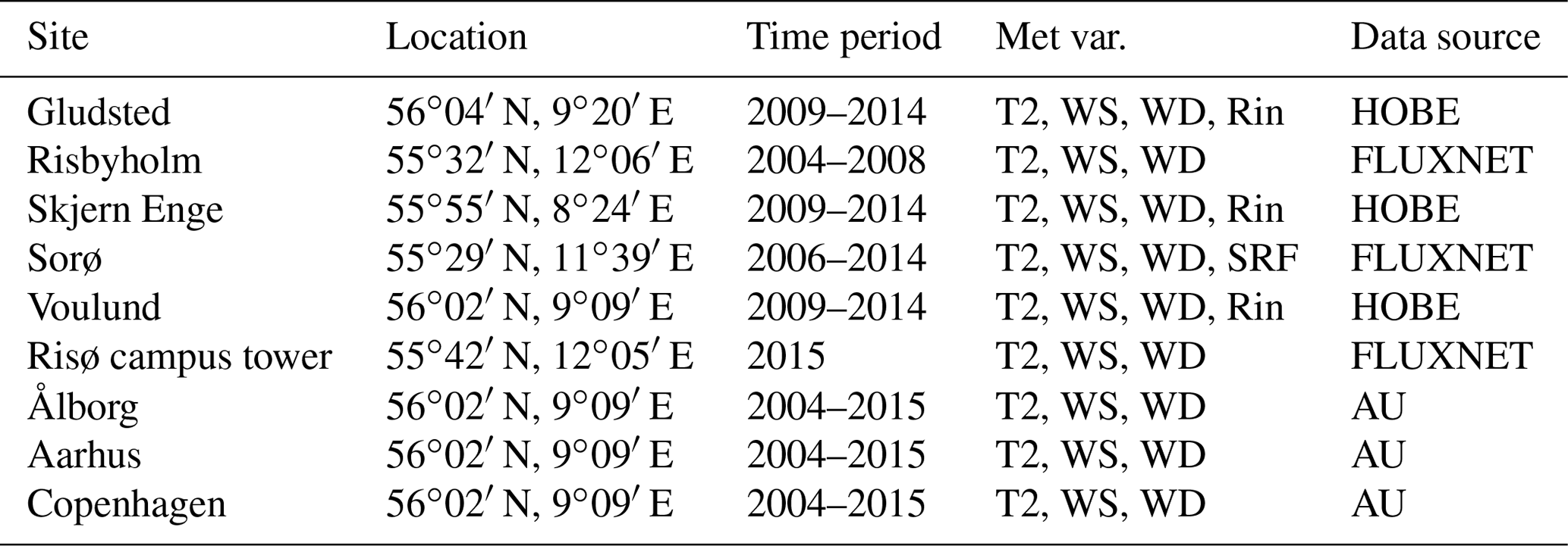
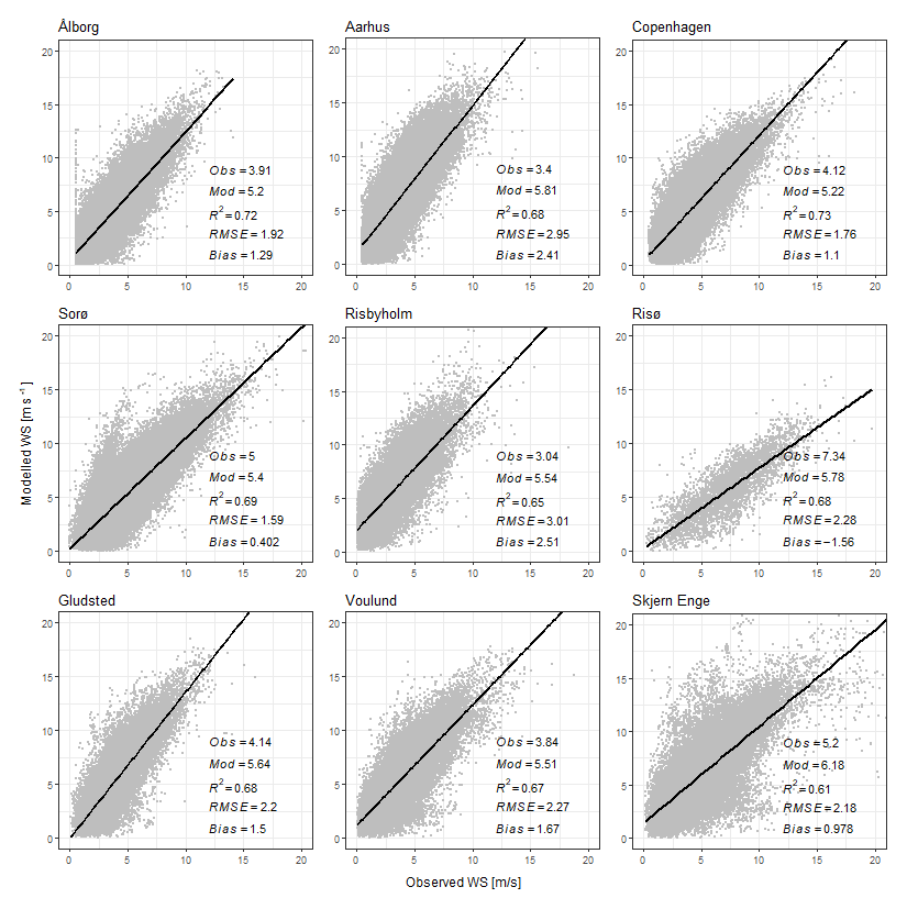
Figure 2Scatter plots of measured versus modelled 10 m wind velocity for the nine sites used for evaluation of the meteorological drivers. Hourly average values are used for both simulated and measured wind velocities. Observed average wind velocity (Obs), simulated average wind velocity (Mod), correlation squared (R2), root-mean-square error (RMSE) and bias are shown for each site.

Figure 3Scatter plots of measured versus modelled 2 m temperatures for the nine sites used for evaluation of the meteorological drivers. Hourly average values are used for both simulated and measured temperatures. Observed average 2 m temperature (Obs), simulated 2 m temperature (Mod), correlation squared (R2), root-mean-square error (RMSE) and bias are shown for each site.
Only one site had available surface pressure measurements, and high correlation of R2=0.99 was obtained with the simulation surface pressures, indicating that WRF was capable of reproducing the actual pressure system across the study region (Fig. S4). Comparisons of wind velocities and wind rose likewise indicate that WRF captured the general atmospheric flow patterns, though the overestimated wind velocities might induce atmospheric mixing too quickly. The simulated mixing layer heights have previously been evaluated, and although the diurnal boundary layer dynamics were reproduced together with the rectifier effect, problems with accurately modelling the nighttime boundary layer were observed, possibly overestimating nighttime surface concentrations of CO2 (Lansø, 2016). Moreover, long-range transport and boundary conditions of atmospheric CO2 concentrations have previously been shown to be captured by the model system across northern Europe, where the current study area is positioned, using observations from Mace Head, Pallas, Westerland, the oil and gas platform F3, Lutjewad, and Östergarnsholm (Lansø et al., 2015).
When evaluating the meteorological variable also important for the biospheric model component, the surface temperature showed high correlation with R2 above 0.93 for all sites (Fig. 3). The total short-wave incoming radiation (Rin) mirrors the measured Rin from the three HOBE sites but is overestimated during summer by WRF (Fig. S5). The values of photosynthetic active radiation (PAR) passed to SPA from DEHM might thus be overestimated, as PAR is proportional to Rin. However, in SPA there is a cap on the limiting carboxylation rate in the calculation of the photosynthesis, and the effect of the overestimated PAR can thus be limited. Precipitation was lacking from all sites, but the annual accumulated modelled precipitation at the nine sites follows the countrywide annual estimates (Cappelan et al., 2018), however, with higher values for the westernmost sites, since many frontal systems enter Denmark from the west (Fig. S6).
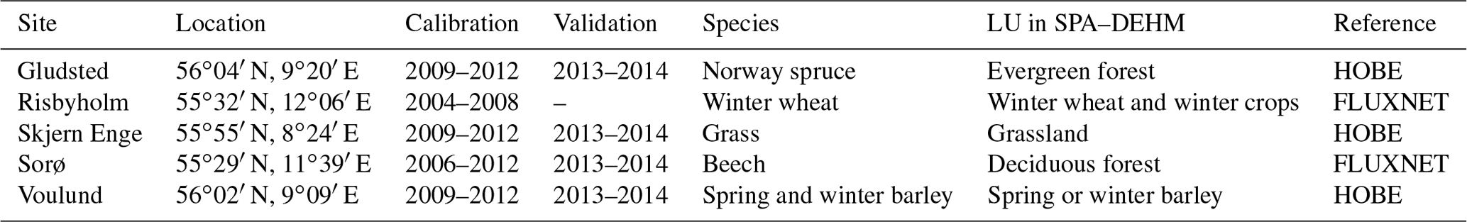
Table 2Location, species and land cover classification in the model system for the five Danish eddy covariance (EC) sites used for calibration and validation of SPA.
3.2 SPA
SPA is a mechanistic terrestrial biosphere model (Williams et al., 1996, 2001). SPA has a high vertical resolution with up to 10 canopy layers (Williams et al., 1996), allowing for variation in the vertical profile of photosynthetic parameters and multi-layer turbulence (Smallman et al., 2013). Within the soil, up to 20 soil layers can be simulated (Williams et al., 2001). The radiative transfer scheme estimates the distribution of direct and diffuse radiation and sunlit and shaded leaf areas (Williams et al., 1998). SPA uses the mechanistic Farquhar model (Farquhar and von Caemmerer, 1982) of leaf-level photosynthesis and the Penman–Monteith model to represent leaf-level transpiration (Jones, 1992). Photosynthesis and transpiration are coupled via a mechanistic model of stomatal conductance, where stomatal opening is adjusted to maximise carbon uptake per unit of nitrogen within hydraulic limitations, determined by a minimum leaf water potential tolerance, to prevent cavitation.
Ecosystem carbon cycling and phenology is determined by a simple carbon cycle model (DALEC; Williams et al., 2005), which is directly coupled to SPA. DALEC simulates carbon stocks in foliage, fine roots, wood (branches, stems and coarse roots), litter (foliage and fine roots) and soil organic matter (including coarse woody debris). Photosynthate is allocated to autotrophic respiration and living biomass via fixed fractions, while turnover of carbon pools is governed by first order kinetics. In addition, when simulating crops, a storage organ (i.e. the crop yield) and foliage pools that are dead but still standing are added, influencing both radiative transfer and turbulent exchange (Sus et al., 2010).
SPA has been extensively validated against site observations from temperate forests (Williams et al., 1996, 2001), temperate arable agriculture (Sus et al., 2010) and the Arctic tundra (Williams et al., 2000). SPA has more recently been coupled to the Weather Research and Forecasting (WRF) model (Skamarock et al., 2008), and the resulting WRF–SPA model was used in multi-annual simulations over the United Kingdom and assessed against surface fluxes of CO2, H2O and heat, and atmospheric observations of CO2 from aircraft and a tall tower (Smallman et al., 2013, 2014).
SPA needs vegetation and soil input parameters. Initial soil carbon stock estimates were obtained from the Regridded Harmonized World Soil Database (Wieder, 2014). The vegetation inputs and plant traits for SPA were partly taken from previous parameter sets used in SPA but also from the Plant Trait Database (TRY; Kattge et al., 2011) and from literature (Penning de Vries et al., 1989; Wullschleger, 1993). As these parameters and plant traits were determined at various sites that do not necessarily correspond to Danish conditions, a calibration of the vegetation inputs to SPA was conducted for Danish eddy covariance (EC) flux sites (Table 2). Only data from five sites were available, and these were divided in two sets – one for calibration (all available observations before 2013) and the other for validation (all available observations from 2013 and 2014).
In the innermost nest of DEHM for the area of Denmark, a coupling was made between DEHM and SPA. Thus, the coarser optimised biospheric fluxes from CT2015 were, for Denmark, replaced by hourly SPA simulated CO2 fluxes. With this change, the spatial resolution for the biosphere fluxes was increased from 1∘ × 1∘ to 5.6 km × 5.6 km, allowing for a better representation of the Danish surface and hence also the biospheric fluxes.
On an hourly basis, DEHM provides atmospheric CO2 concentrations and the meteorological drivers obtained from WRF to SPA, while SPA returns net ecosystem exchange (NEE) to DEHM each hour.
3.2.1 SPA calibration
The calibration was conducted by selecting a set of inputs parameters (plant traits, carbon stocks, etc.), and for each parameter, five values within a realistic range were chosen. Next, 200 SPA simulations with randomly chosen parameter values were conducted. These results were statistically evaluated against observations of NEE from the different flux sites, with the aim of selecting the parameter combination with the lowest root-mean-square error (RMSE) in combination with highest correlation that captured the observed variability and onset of the growing season. However, it was not always possible to have all these conditions satisfied (e.g. Fig. S7). Based on this random parameter testing, it was possible to choose the best set of realistic vegetation input parameters that could improve the model performance at the Danish sites. The best found vegetation parameters values corresponded in some cases to the values already applied in SPA for the given land cover.
3.2.2 SPA evaluation
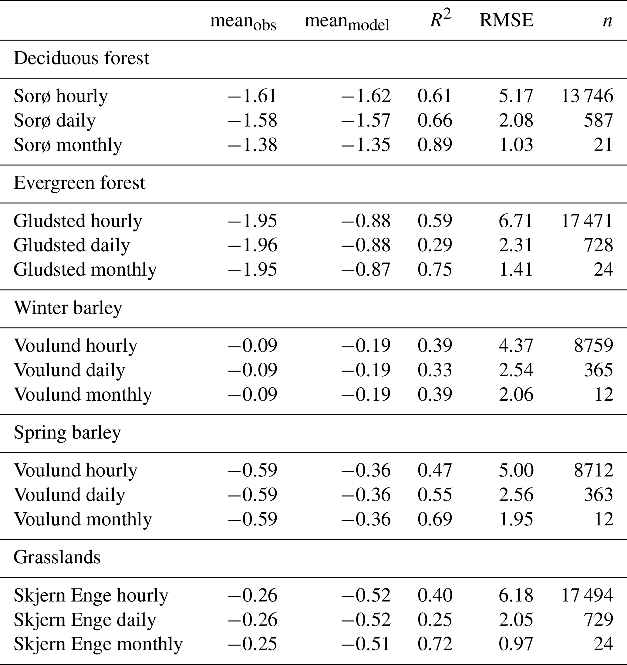
Comparing to observations of NEE, SPA was, in general, able to capture the phenology and seasonal cycle throughout the entire simulation period (Fig. 4). Correlations and RMSEs between the model and the independent data from the validation period (Fig. 4) likewise indicate a good model performance. At Sorø, variability, as inferred from the standard deviations, the amplitude and the onset of the growing season were reproduced well by SPA. However, difficulties with simulating the evergreen forest at Gludsted are evident, with more variation modelled than given by the observations and a lag of the start of the growing season when compared to the observations. The evergreen plant functional type in SPA lacks a labile or non-structural carbohydrate store needed to drive rapid leaf expansion with the onset of spring; instead leaf expansion is dependent on available photosynthate in a given time step. Therefore, SPA's leaf area index (LAI) is lower early in the growing season, resulting in a biased slow photosynthetic activity and an underestimation in the magnitude of NEE, as seen at Gludsted (Fig. 4). Voulund alternates between winter and spring barley for the calibration period starting with winter barley in 2009. Note that the whole observed time series of NEE at Voulund is shown together with model NEE of both winter and spring barley (Fig. 4c and d). While the phenology and amplitude are captured well for spring barley at Voulund, SPA is not able to capture the seasonal amplitude of the winter barley that seems to be more sensitive to the meteorological drives, and seasons with harder winters had lower NEE peaks in summer (winter 2010–2011 and 2012–2013). At the grassland site Skjern Enge, NEE is reasonably modelled for winter, spring and the first part of the summer. The difficulties for late summer and autumn arise from the management practices at the site, where both grazing and grass cutting are conducted, limiting NEE (Herbst et al., 2013). Although grazing is included in SPA, it does not simulate the same reduction in NEE.
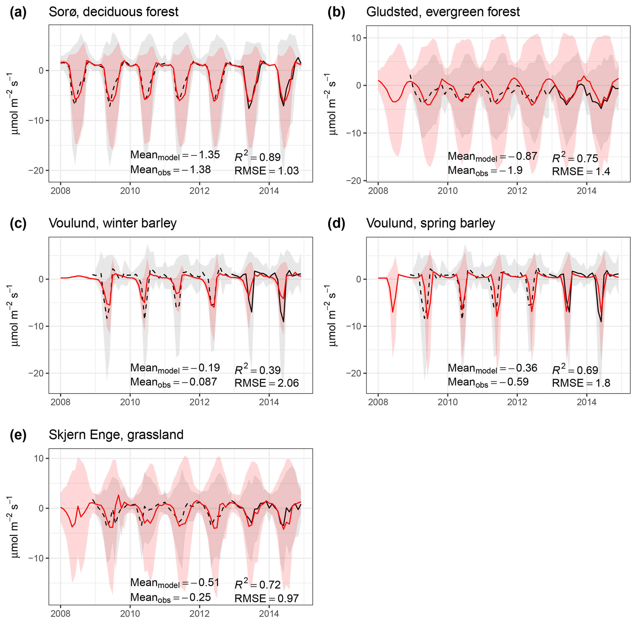
Figure 4Monthly averaged values of measured (black dashed, calibration period; black solid, validation period) and simulated (red) net ecosystem exchange (NEE) for the Danish EC sites with measurements in the simulation period. The shaded areas show the standard deviations for the modelled and measured NEE calculated using hourly fluxes. The model mean (Meanmodel), observational mean (Meanobs), correlation squared (R2) and root-mean-square error (RMSE) for the validation period (2013 and 2014) are shown for each site.
Examining the performance of SPA at a higher temporal resolution (Table 3), the correlations are better for hourly values than daily for the land cover classification having problems with the phenology (evergreen forest and winter barley) because SPA is capable of reproducing the diurnal variability. For the remaining land cover classifications, R2 and RMSE are improved when going from hourly to monthly averages of NEE. Zooming in on shorter time windows, the timing of the diurnal cycle is in accordance with measured NEE (see e.g. Fig. S9), but the amplitude is underestimated by SPA.
Table 3Statistic metrics for the validation period (2013–2014) for the fives sites that have measurements of NEE during the validation period for hourly, daily and monthly values. Measured mean (meanobs), modelled mean (meanmodel), correlation squared (R2) and root-mean-square error (RMSE) are shown for each site and temporal resolution.
The model system was run from 2008 to 2014, with the first 3 years regarded as a spin-up period. In the following sections the terrestrial and marine surface fluxes will be presented first, followed by measurements of atmospheric CO2 from the Risø campus tower that will be used to assess the performance of the DEHM–SPA system and evaluate local impacts from fjord systems on atmospheric CO2 concentrations.
4.1 Surface fluxes
4.1.1 Biospheric fluxes
As shown in Fig. 5, SPA simulates an east–west gradient in NEE for both January and July in 2011. Larger values of NEE are found in the western part of Denmark, while the islands and eastern Jutland have lower biosphere fluxes. This gradient follows the distribution of the individual land cover classifications (Fig. S8), their phenology and productivity but also reflects the urbanisation, which is denser in the eastern part of the country. During January, total ecosystem respiration dominates NEE. Evergreen forests and grasslands are represented well in western Jutland, and even though these land cover classes have gross primary production (GPP), they are still dominated by total ecosystem respiration, but their total ecosystem respiration can be higher than the other land cover classifications because of the contribution from the autotrophic respiration that depends on GPP in SPA. During July, the productivity is at its highest for all land cover classes dominating total ecosystem respiration, resulting in negative NEE (Fig. 6), and the gradient across the country is more likely to be a result of the urbanisation.
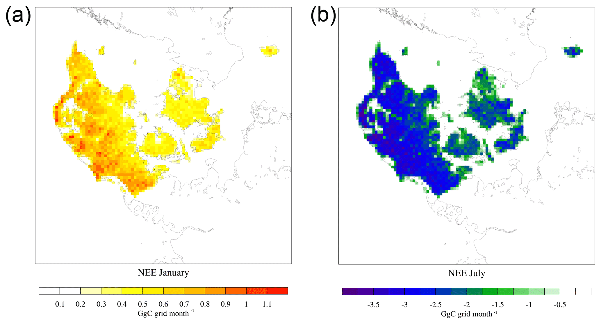
Figure 6 shows the average monthly contribution from each land cover classification to the countrywide NEE, which inherently follows their productivity but also reflects the area covered by each land cover type, with highest peaks for winter wheat and grasslands during June. During winter, the spread amongst the land cover classifications is smaller but still has numerically larger monthly fluxes for the land cover classifications with largest area. Integrating over all land cover classifications, the Danish terrestrial land surfaces are a net source of CO2 to the atmosphere in the months from October to April, with the highest release of 1063±154 GgC per month in December. From May to September, the biosphere is a net sink with a maximum uptake in June of GgC. The total surface exchange of CO2 between the atmosphere and Danish biosphere is GgC yr−1, where winter wheat has the largest contribution with GgC yr−1.
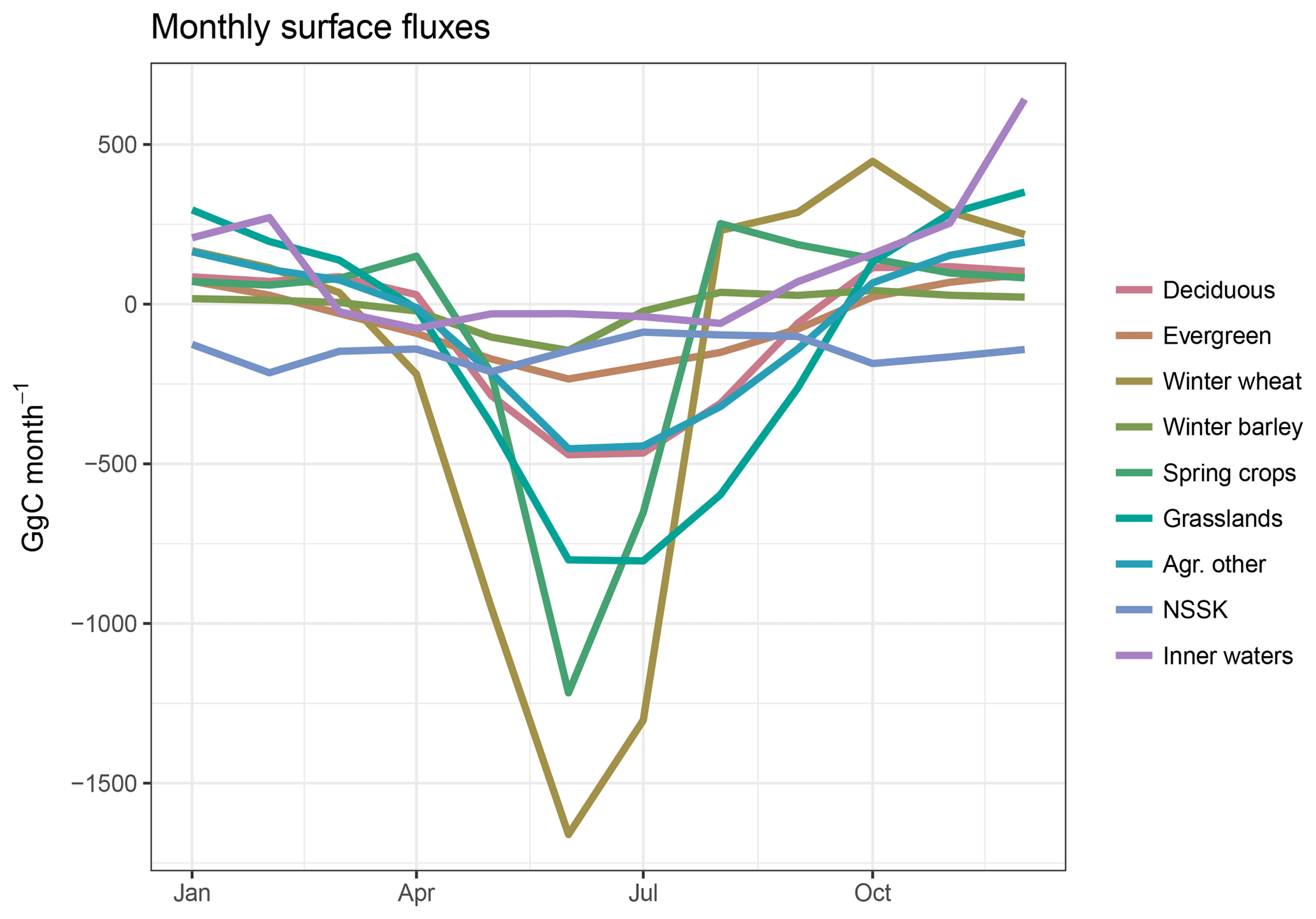
Figure 6Total monthly average of NEE for each land cover classification for the simulation period of 2011–2014 together with the monthly air–sea CO2 from the Danish marine areas that have been divided into the North Sea and Skagerak (NSSK) and Kattegat and the Danish straits (inner waters).
4.1.2 Marine fluxes
The air–sea CO2 exchange in the Danish inner waters experiences large seasonal variations, while the variations in the North Sea are less pronounced, as illustrated by Fig. 7. The mineralisation in winter increases the surface water pCO2 in the Danish inner waters, resulting in outgassing of CO2 to the atmosphere, while uptake occurs during spring and summer months following the decrease in surface water pCO2 due to biological activities.
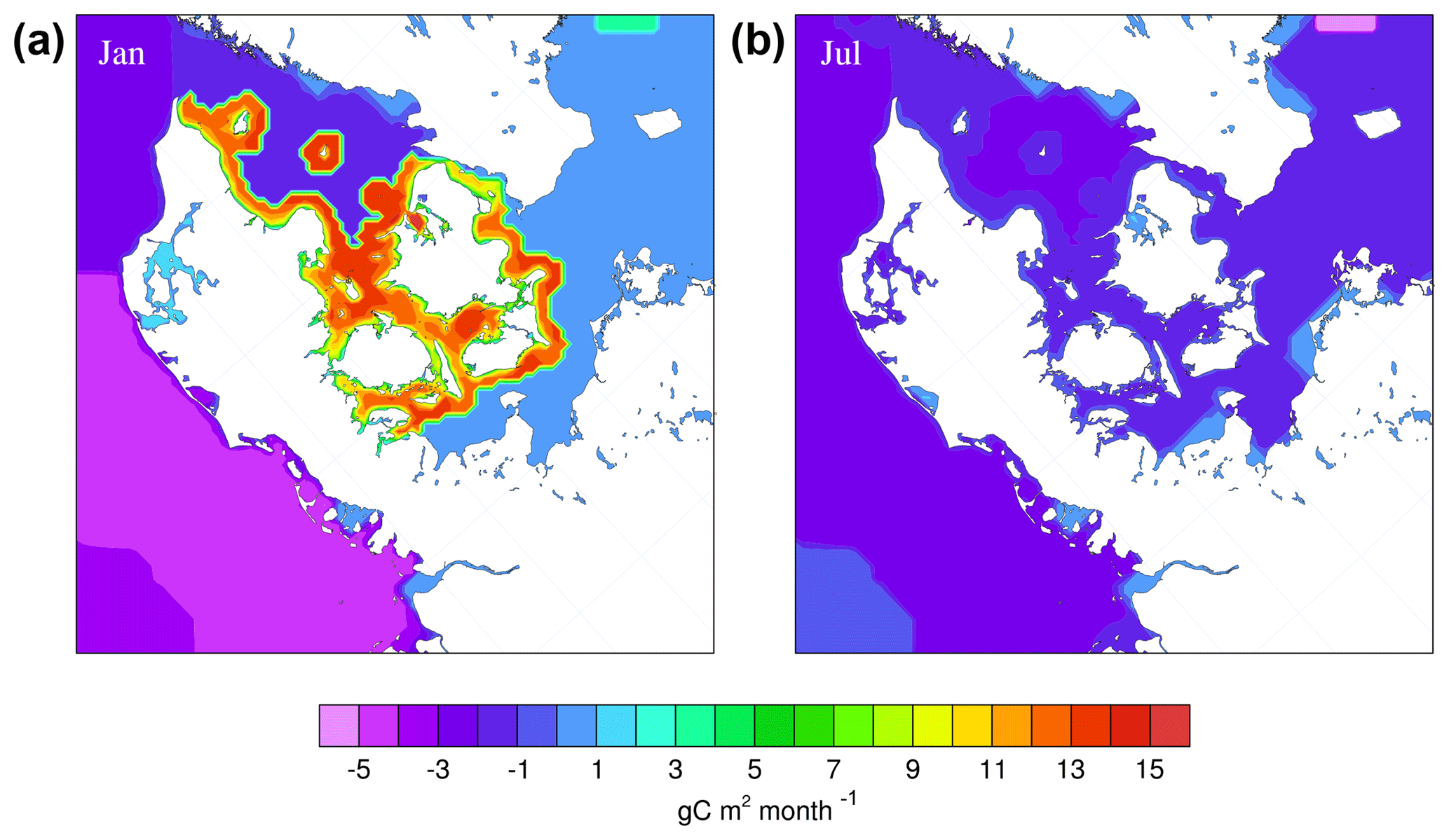
Figure 7Simulated air–sea CO2 exchange within the model framework for January (a) and July (b) 2011. The spatial resolution follows those of nest 4 from the DEHM model (i.e. 5.6 km × 5.6 km). The formulation by Ho et al. (2006) was used to calculate the air–sea CO2 exchange.
The simulated annual air–sea CO2 exchange in the 105 000 km2 covered by the Danish EEZ amounts to −422 GgC yr−1. However, this number masks large spatial differences and monthly numerical larger fluxes (Fig. 6). While the North Sea area contained within the EEZ continuously had uptakes in the range −73 to −191 GgC per month with an accumulation of 1765 GgC yr−1, the fluxes from the near-coastal Danish inner waters varied in the range −46 to 540 GgC per month, releasing 1343 GgC yr−1 to the atmosphere.
4.2 Atmospheric CO2 concentrations
The time series of measured and simulated CO2 show good agreement (Fig. 8) with R2=0.77 and RMSE = 4.87 ppm for daily averaged time series, demonstrating that the model is capable of capturing the synoptic scale variability. Also, good statistical measures are obtained for the hourly time series with R2=0.71 and RMSE = 5.95 ppm, but the short-term variability was not always fully captured by the model. All in all, the evaluation shows that the model can capture the overall variability in the atmospheric CO2 concentrations and fluxes. Moreover, the higher resolution in both the transport model and surface fluxes results in a better model performance in simulating atmospheric CO2 concentrations (Fig. S10).

Figure 8Hourly averages and daily averages of modelled and continuously measured atmospheric CO2 at the Risø site for 2013–2014. The trends have been removed from the time series.
To investigate the origin of the CO2 simulated at the Risø site, concentration rose plots of simulated atmospheric CO2 have been made (Fig. 9). The concentration rose shows the wind direction and associated CO2 concentrations. Division has been made between seasons and daytime and nighttime values, both showing distinct seasonal and diurnal patterns. The highest values of CO2 are obtained during winter, where very little diurnal variation is seen. During summer the lowest values are obtained in particular during daylight, when photosynthesis occurs.
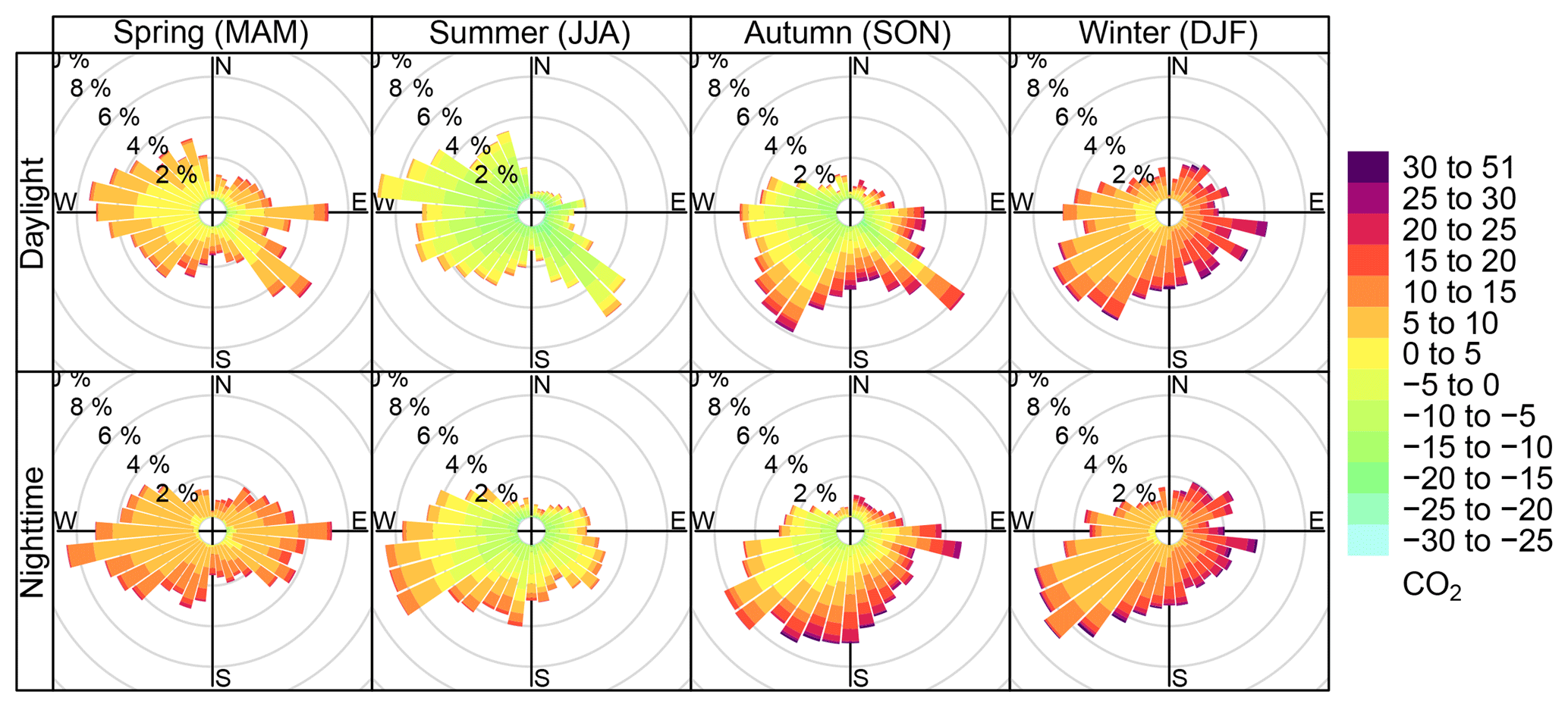
Figure 9Concentration roses of modelled atmospheric CO2 (ppm) at the Risø site for 2011–2014. The wind direction is split into 10∘ intervals, and the frequency is indicated by the concentric circles. The colours indicate the CO2 concentrations with mean removed that have been transported to the site from the given wind directions.
The individual contribution from fossil fuel emissions, marine and biospheric exchanges to the atmospheric CO2 (see Figs. S11–S13) indicate that the biosphere contributes most to the variations simulated at Risø (Fig. S12) – both seasonally and daily. Emissions of fossil fuel experience little diurnal variability, but seasonally having the greatest contribution during autumn and winter (Fig. S11). The highest values are seen originating from the sectors encapsulating the city of Roskilde and the capital region. In all seasons, the simulated oceanic contribution is negative, i.e. indicating uptake of atmospheric CO2, but the marine contribution is small, with little variation (Fig. S13). The less negative values in autumn and winter may be a result of the simulated outgassing of CO2 from the Baltic Sea and Danish inner waters during the winter season (Lansø et al., 2015), which, however, is still dominated by the uptake by global open oceans.
The local impact from Roskilde Fjord is difficult to detect in the marine concentration plots. Flux measurements at Roskilde Fjord have shown uptake of CO2 during spring while release of CO2 in the remaining seasons (Mørk et al., 2016), which is accurately captured by the modelling system (Lansø et al., 2017). A footprint analysis of the Risø tower has shown that the fluxes from Roskilde Fjord have a contribution to the total CO2 flux measured at the top of the 118 m high tower, but it is only minor, since fluxes over water are typically an order of magnitude smaller than fluxes over land (Sogachev and Dellwik, 2017). Therefore, we investigated a period with observed large outgassing from Roskilde Fjord – a storm event in October 2013 that was observed to increase the monthly release of CO2 in the fjord by 66 % (Mørk et al., 2016). The storm event passed Denmark on 28 October 2013, and at 06:00 UTC southerly winds transport air masses with higher CO2 towards the Risø site (Fig. 10a), while at the same time a detectable increase in the oceanic contribution to the CO2 concentration at the Roskilde Fjord system is seen (Fig. 10b). The model system simulates the small peak in the observed atmospheric CO2 concentrations for 28 October (Fig. 11a) at the Risø site, but distinguishing between contributions from fossil fuel emissions, the biosphere and the ocean to the atmospheric CO2 concentration at Risø (Fig. 11b) reveals no oceanic impact, and hence there is no apparent influence from Roskilde Fjord during the storm event.
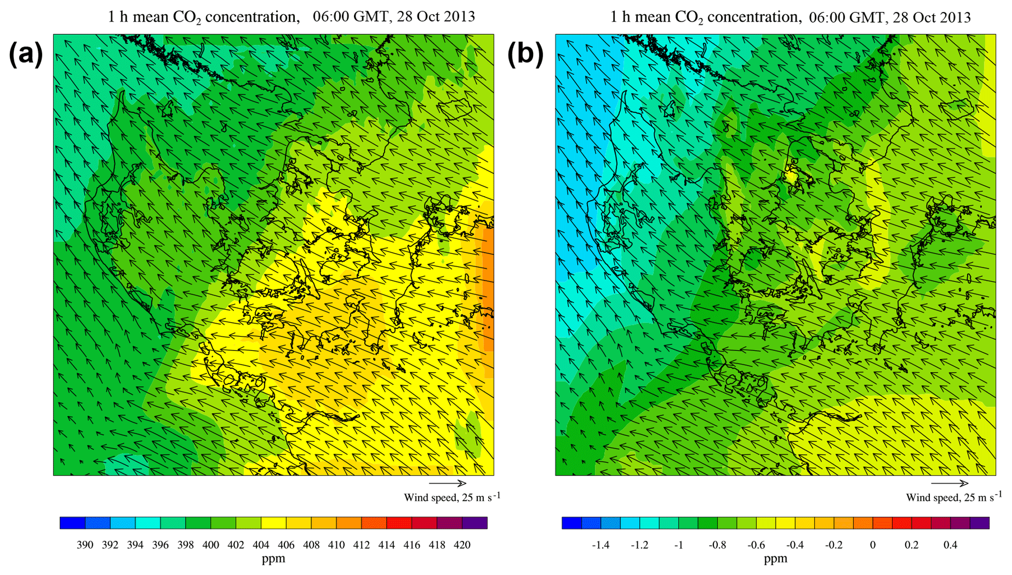
Figure 10(a) Hourly averages of atmospheric CO2 concentrations including the annual background across Denmark on 28 October 2013 06:00 UTC during the October storm. (b) The contribution from the marine exchange alone to the hourly averaged atmospheric CO2 concentration on 28 October 2013 06:00 UTC. The less negative values at the Roskilde Fjord system indicate release of CO2 to the atmosphere.
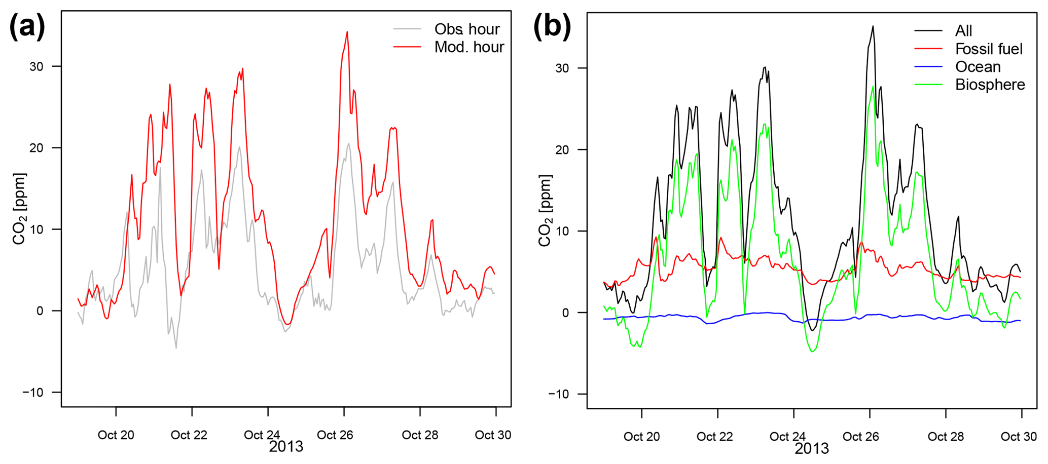
Figure 11(a) Hourly averages of modelled and continuously measured atmospheric CO2 at the Risø site for 19–29 October 2013 with annual means removed. (b) Contributions from fossil fuel emission, oceanic surface exchange and biospheric surface exchange to the atmospheric CO2 concentration, shown as 1 h averages of modelled concentrations at the Risø site for the same period.
5.1 Surface fluxes
The simulated annual uptake by deciduous forest of gC m−2 yr−1 for the period 2011–2014 is within the observed range of annual estimated NEE at Sorø from 1996 to 2009, spanning from 32 to −331 gC m−2 yr−1 (Pilegaard et al., 2011). Improvements to the evergreen plant functional type in SPA are needed, and an addition of a labile pool to the evergreen carbon assimilation would omit the seasonal lag (Williams et al., 2005). Such adjustments have already been made to the DALEC carbon assimilation system utilised by SPA (Smallman et al., 2017), substantially improving the representation of terrestrial phenology but not yet being incorporated into SPA. The estimated uptake of gC m−2 yr−1 is in the low range of previous estimates of temperate evergreen forests with −402 gC m−2 yr−1 (Luyssaert et al., 2007) and Danish evergreen plantations of −503 gC m−2 yr−1 (Herbst et al., 2011). This could be caused by the slow leaf onset in spring, inhibiting the productivity at the beginning of the growing season.
Previous annual estimates at Danish agricultural field sites found carbon uptake of −31 gC m−2 yr−1 estimated from a mixed agricultural landscape (Soegaard et al., 2003) and −245 gC m−2 yr−1 at a winter barley site (Herbst et al., 2011). The SPA–DEHM model system simulated annual uptakes for winter wheat of gC m−2 yr−1, and spring crops of gC m−2 yr−1, while winter barley had a smaller uptake of gC m−2 yr−1 with large standard deviation potentially resulting in small annual releases. The calibration and validation (Fig. 4c) show difficulties in simulating the observed NEE during growing seasons for winter barley, particularly after cold and snow-covered winters. As pointed out in previous studies, the crop modelling component in SPA could likewise be improved, e.g. by inclusion of intra-seasonal crops (Smallman et al., 2014).
The current study estimated the Danish grasslands to be a sink of CO2 with gC m−2 yr−1, which is similar, albeit slightly smaller, than the −267 gC m−2 yr−1 observed at the Skjern Enge grassland site during 2009–2011 (Herbst et al., 2013) and the −312 gC m−2 yr−1 observed at the Lille Valby grassland site, Denmark (Gilmanov et al., 2007). The European grassland study by Gilmanov et al. (2007) found large variation in annual fluxes from grassland driven by environmental conditions and management practices at the sites varying from 171 to −707 gC m−2 yr−1, but with most sites having an annual uptake of carbon. As seen in Fig. 4e, more work on grassland calibration could have been done, but the conditions and management regimes at Skjern Enge do not necessarily fit the rest of the Danish grasslands. With the chosen parameters, very comparable results were obtained, indicating that such an additional calibration might not be advantageous.
A tilling approach has been used for the land cover classification in the SPA–DEHM modelling framework, including sub-grid heterogeneity in the model system. However, the seven land cover classes do not fully encompass the ecosystem variability in Denmark. Both grassland and agricultural other cover a broad range of subcategories, with both heather and meadow included in the grassland class, while agricultural other contains, for example, vegetables fields, hedgerows, woodland patches and uncultivated land, highlighting the need to adopt approaches allowing for generating novel spatially varying parameter sets (Bloom et al., 2016). Moreover, large urbanised areas are not accounted for in the current classes either. Adding more land cover classifications could give a better and more realistic surface description, if data for both calibration and validation for the lacking land cover classes, preferably from a similar climatic region to Denmark, were available.
Compatible marine fluxes to previous estimates are obtained for the study region. On an annual basis, the Danish inner waters were found to be a source of 30 gC m−2 yr−1, which agrees with most previous studies. Wesslander et al. (2010) estimated Kattegat to act as a small sink of −14 gC m−2 yr−1 based on measurements of water chemistry, while Norman et al. (2013), on the contrary, found a release of 19 gC m−2 yr−1 using a biogeochemical model of the Baltic Sea. Measurements from Danish fjords, on the other hand, consistently point towards these marine areas being annual sources of CO2, with values in the range of 41 to 104 gC m−2 yr−1 (Gazeau et al., 2005; Mørk et al., 2016). The current study estimates the North Sea to be a sink of −29 gC m−2 yr−1, which is very close to previous estimates, both measured and modelled, of −20 and −25 m−2 yr−1 (Thomas et al., 2004; Prowe et al., 2009).
5.2 Atmospheric CO2 and land–sea signals
WRF is in general capable of simulating the observed wind patterns, while the overestimation of the wind velocity could lead to an overestimation of the atmospheric mixing. However, the SPA–DEHM modelling system resembles the synoptic and diurnal variability in the atmospheric CO2 concentrations measured at Risø campus tower site. The variability at the Risø site is dominated by the biospheric impact and fossil fuel emissions of CO2. The signal from Roskilde Fjord is difficult to detect in the simulated CO2 concentrations. Even when the marine contribution to the atmospheric concentration alone is examined, the Roskilde Fjord signal is hard to distinguish at the Risø campus tower. Moreover, sea breezes from the narrow Roskilde Fjord might be difficult to detect by the model system with its 5.6 km horizontal resolution.
As Roskilde Fjord previously was found by a footprint analysis to have an impact on the atmospheric CO2 concentration at the top of the tower (Sogachev and Dellwik, 2017), a period with observations of large outgassing from Roskilde Fjord was examined to more clearly envision its impact in the simulated concentration fields. Both the simulated and observed atmospheric CO2 increased during the storm event on 28 October (Fig. 10a), but no concurrent increase was seen in the oceanic contribution to atmospheric CO2 at the Risø site (Fig. 10b). This might be explained by the southerly winds that transported the CO2 released from the fjord northward and away from the Risø campus tower, which is positioned in the southern part of the fjord. Moreover, in this study the increased flux from Roskilde Fjord was only caused by increased wind speed together with the imposed diurnal cycle of marine pCO2 (the diurnal amplitude for October was approximately 10 µatm), while measurements suggested that an increase in surface water pCO2 of approximately 300 µatm also sustained the observed CO2 flux (Mørk et al., 2016). The lack of such an increase in surface water pCO2 in the current modelling study could explain why no impact on the simulated atmospheric CO2 is seen from the marine component during the storm event. Thus, the results could indicate that (i) the narrow Roskilde Fjord was not sufficiently resolved in the current model framework, where the horizontal grid resolution is 5.6 km × 5.6 km, (ii) the surface water pCO2 was not described in enough detail in the model system, (iii) Roskilde Fjord is not in the footprint of the tower during the storm event or (iv) the fjord only has a minor impact on the atmospheric CO2 concentrations at Risø.
However, the air–sea CO2 exchange from the Danish inner waters (including all fjord, inner straits and Kattegat) has an impact during winter. Between November and February, the air–sea fluxes from the Danish inner water correspond to 23 %–60 % of the monthly NEE (see Fig. 6). Moreover, the higher values of about 0.5 ppm in the concentration roses of the marine contribution to the atmospheric CO2 concentrations at the Risø campus tower site in winter likewise emphasise the marine impact, though the outgassing from the neighbouring Baltic Sea also has a contribution. Although the annual total numerical marine fluxes of 1765 gC yr−1 from the North Sea and 1343 gC yr−1 from the Danish inner waters are comparable to the sizes of annual NEE for individual land cover classifications (e.g. deciduous at −987 gC yr−1, evergreen at −665 gC yr−1 and grasslands at −1467 gC yr−1), the air–sea CO2 fluxes are 1 order of magnitude smaller than the biospheric fluxes, with 30 gC m−2 yr−1 for the Danish inner waters and −29 gC m−2 yr−1 for the North Sea and Skagerak.
5.3 Uncertainties in relation to surface exchanges of CO2
Some of the largest uncertainties lie in the parameters underlying the terrestrial carbon cycle, in particular those governing allocation to plant tissues and their subsequent turnover. Most often these are based on maps of land cover or plant functional type, but parameter estimation via data assimilation analysis has shown substantial spatial variation in terrestrial ecosystem parameters within plant functional type groupings, with consequences for carbon cycling predictions (Bloom et al., 2016). Increasing the quantity and type of observations available for data assimilation systems can have a significant impact on reducing uncertainty of model process parameters and simulated fluxes (Smallman et al., 2017). In particular, availability of repeated above-ground biomass estimates was able to half the uncertainty of net biome productivity estimates for temperate forests (Smallman et al., 2017). Above-ground biomass estimates are currently available from remote sensing sources (e.g. Thurner et al., 2014; Avitabile et al., 2016), with future planned missions such as the ESA Biomass mission (Le Toan et al., 2011) and NASA GEDI (https://gedi.umd.edu/, last access: January 2019) providing high-quality observations over the tropics and global scales, respectively.
While SPA also uses DALEC to simulate carbon allocation and turnover, it is currently impractical to conduct a similar data assimilation analysis to optimise DALEC (or SPA) parameters based on comparison with observations of atmospheric CO2 concentrations, as this would require repetition of computationally intense simulations of atmospheric transport. While conducting such an analysis remains a future ambition, we consider it to be out of the scope of the current study, since the terrestrial surface fluxes in this study are constrained by one data stream consisting of EC measurements. This study has focussed on surface fluxes over a relative short time period, and the model framework was capable of producing such fluxes, including their aggregated impact on atmospheric CO2 concentrations (Fig. 4) with R2=0.77 and RMSE = 4.87 ppm for daily values.
Uncertainties of the marine fluxes can be associated with both the choice of transfer velocity parameterisation, choice of the wind speed product and the used surface water pCO2 maps. Sensitivity analysis of global transfer velocity parameterisation based on 14C bomb inventories shows uncertainties of 20 %, while varying the applied wind speed products for these formulation increases the difference in the global annual flux by 40 % (Roobaert et al., 2018). Including empirical formulations of transfer velocity parameterisation in the analysis increased the sensitivity of the wind speed product to nearly 70 %, while the uncertainty of the parameterisation itself rose to more than 200 %. More than a doubling of the annual uptake by the usage of different transfer velocity formulations has likewise been shown for the study region (Lansø et al., 2015), while the choice of the surface water pCO2 map could change the study region from an annual sink to source of atmospheric CO2 (Lansø et al., 2017). As shown by Roobaert et al. (2018) the ERA-Interim and the transfer velocity formulation by Ho et al. (2006) used in the present study have a combined uncertainty estimate around 20 %. The improved data-driven near-coastal Danish pCO2 climatology better reflects the observed spatial dynamics and seasonality in the Danish inner waters (Mørk, 2015), albeit not diminishing the uncertainty related to surface maps of pCO2 but reducing it.
By usage of the designed mesoscale modelling framework, it was possible to get detailed insight into the spatio-temporal variability in the Danish surface exchanges of CO2 and the relative contribution from the different surface types. The simulated biospheric fluxes experienced an east–west gradient corresponding to the distribution of the land cover classes, their biological activity and the urbanisation pattern across the country. The relative importance of the seven land cover classes varied throughout the course of the year. Grasslands had a high contribution to the monthly NEE through all seasons, while croplands influence grew from March to July. On an annual basis, winter wheat had the largest impact on the biospheric uptake, with −2342 GgC yr−1. However, the simulated biospheric uptake could benefit both from model improvement and divisions into more land cover classes. The marine fluxes, being subdivided into the North Sea including Skagerak and the Danish inner waters, had annual fluxes of opposite signs, with the North Sea being a continuous sink of atmospheric CO2 and the Danish inner waters experiencing small uptake in summer and release of CO2 during winter resulting in a total marine annual uptake of −422 GgC yr−1.
Good accordance between simulated and observed concentrations was found between modelled and observed atmospheric CO2 concentrations for 2013 and 2014 at the Risø campus tower. The origin of the modelled CO2 concentrations at Risø varied, with biospheric fluxes having the largest impact on diurnal variability, while on a seasonal scale fossil fuel emissions also had a dominant role. The local impact from Roskilde Fjord was difficult to detect, while regional impact from the Baltic Sea and Danish inner straits is apparent in winter. The results may indicate that Roskilde Fjord and its localised impact (i.e. at the Risø campus tower site) on atmospheric CO2 are not adequately resolved in the current model set-up or only have a modest effect. Numerically, the annual fluxes from the North Sea and the Danish inner water were comparable in size to the annual net terrestrial fluxes from the individual land cover classifications.
In order to further examine the air–sea signal at the complex Risø site surrounded by a mosaic of fjord systems, land masses and the Danish inner water, more model experiments could be made, where a larger focus is put on other marine areas than Roskilde Fjord, e.g. the Danish inner straits, Kattegat and the Baltic Sea. Although the total annual marine flux was small, it disguises large monthly variations, and further investigations could help to understand the carbon dynamics in coastal regions. A runoff component in the modelling system would moreover be beneficial for such studies.
Scientists with an interest in the atmospheric chemical transport model, DEHM, can contact Jesper H. Christensen (jc@envs.au.dk) with enquiries. Scientists with an interest in the soil–plant–atmosphere model, SPA, can visit its web page (https://www.geos.ed.ac.uk/homes/mwilliam/spa.html, last access: January 2019) or contact Mathew Williams (mat.williams@ed.ac.uk).
The supplement related to this article is available online at: https://doi.org/10.5194/bg-16-1505-2019-supplement.
ASL and CG designed the experiment. ASL was responsible for coupling the model, which JHC assisted with, and running the experiments. LLS made contributions to the marine set-up, while MW and TSL were responsible for SPA. KP conducted the atmospheric measurements of CO2 at the Risø campus tall tower. All authors contributed to the discussion of the results and the preparation of the paper.
The authors declare that they have no conflict of interest.
This study was carried out as part of a PhD study within the Danish ECOCLIM project funded by the Danish Strategic Research Council (grant no. 10-093901). CarbonTracker CT2015 results that were provided by the NOAA ESRL, Boulder, Colorado, USA, from the website http://carbontracker.noaa.gov (last access: January 2016) have contributed to this work. Emission inventories form IER, EDGAR and Aarhus University have likewise made an important contribution. This study has been supported by the TRY initiative on plant traits (http://www.try-db.org, last access: June 2015). The TRY initiative and database is hosted, developed and maintained by Jens Kattge and Gerhard Bönisch (Max Planck Institute for Biogeochemistry, Jena, Germany). TRY is currently supported by DIVERSITAS–Future Earth and the German Centre for Integrative Biodiversity Research (iDiv) Halle–Jena–Leipzig. Moreover, this work used eddy covariance data acquired and shared by the Danish Hydrological Observatory, HOBE, founded by the Villum Foundation and by the FLUXNET community. The FLUXNET eddy covariance data processing and harmonisation were carried out by the European Fluxes Database Cluster, AmeriFlux Management Project, and Fluxdata project of FLUXNET, with the support of CDIAC and ICOS Ecosystem Thematic Center and the OzFlux, ChinaFLUX and AsiaFlux offices. We are grateful for many fruitful discussions regarding the atmospheric measurements of CO2 at the Risø tall tower and its applications in a modelling framework with Ebba Dellwik at DTU Wind Energy.
This paper was edited by Trevor Keenan and reviewed by two anonymous referees.
Ahmadov, R., Gerbig, C., Kretschmer, R., Körner, S., Neininger, B., Dolman, A. J., and Sarrat, C.: Mesoscale covariance of transport and CO2 fluxes: Evidence from observations and simulations using the WRF-VPRM coupled atmosphere-biosphere model, J. Geophys. Res.-Atmos., 112, d22107, https://doi.org/10.1029/2007JD008552, 2007. a, b
Ahmadov, R., Gerbig, C., Kretschmer, R., Körner, S., Rödenbeck, C., Bousquet, P., and Ramonet, M.: Comparing high resolution WRF-VPRM simulations and two global CO2 transport models with coastal tower measurements of CO2, Biogeosciences, 6, 807–817, https://doi.org/10.5194/bg-6-807-2009, 2009. a, b
Avitabile, V., Herold, M., Heuvelink, G. B. M., Lewis, S. L., Phillips, O. L., Asner, G. P., Armston, J., Ashton, P. S., Banin, L., Bayol, N., Berry, N. J., Boeckx, P., de Jong, B. H. J., DeVries, B., Girardin, C. A. J., Kearsley, E., Lindsell, J. A., Lopez-Gonzalez, G., Lucas, R., Malhi, Y., Morel, A., Mitchard, E. T. A., Nagy, L., Qie, L., Quinones, M. J., Ryan, C. M., Ferry, S. J. W., Sunderland, T., Laurin, G. V., Gatti, R. C., Valentini, R., Verbeeck, H., Wijaya, A., and Willcock, S.: An integrated pan-tropical biomass map using multiple reference datasets, Glob. Change Biol., 22, 1406–1420, 2016. a
Bloom, A. A., Exbrayat, J.-F., van der Velde, I. R., Feng, L., and Williams, M.: The decadal state of the terrestrial carbon cycle: Global retrievals of terrestrial carbon allocation, pools, and residence times, P. Natl. Acad. Sci. USA, 113, 1285–1290, https://doi.org/10.1073/pnas.1515160113, 2016. a, b
Brandt, J., Silver, J. D., Frohn, L. M., Geels, C., Gross, A., Hansen, A. B., Hansen, K. M., Hedegaard, G. B., Skjøth, C. A., Villadsen, H., Zare, A., and Christensen, J. H.: An integrated model study for Europe and North America using the Danish Eulerian Hemispheric Model with focus on intercontinental transport of air pollution, Atmos. Environ., 53, 156–176, https://doi.org/10.1016/j.atmosenv.2012.01.011, 2012. a
Bregman, B., Segers, A., Krol, M., Meijer, E., and van Velthoven, P.: On the use of mass-conserving wind fields in chemistry-transport models, Atmos. Chem. Phys., 3, 447–457, https://doi.org/10.5194/acp-3-447-2003, 2003. a
Broquet, G., Chevallier, F., Rayner, P., Aulagnier, C., Pison, I., Ramonet, M., Schmidt, M., Vermeulen, A. T., and Ciais, P.: A European summertime CO2 biogenic flux inversion at mesoscale from continuous in situ mixing ratio measurements, J. Geophys. Res.-Atmos., 116, D23303, https://doi.org/10.1029/2011JD016202, 2011. a
Cai, W.-J.: Estuarine and Coastal Ocean Carbon Paradox: CO2 Sinks or Sites of Terrestrial Carbon Incineration?, Annu. Rev. Mar. Sci, 3, 123–145, https://doi.org/10.1146/annurev-marine-120709-142723, 2011. a
Cappelan, J., Kern-Hansen, C., Laursen, E. V., Viskum Jørgensen, P. V., and Jørgensen, B. V.: Denmark – DMI Historical Climate Data Collection 1768–2017, Danish Meteorological Institute, p. 111, available at: https://www.dmi.dk/publikationer/ (last access: January 2019), 2018. a
Carslaw, K. S., Lee, L. A., Regayre, L. A., and Johnson, J. S.: Climate models are uncertain, but we can do something about it, EOS, 99, https://doi.org/10.1029/2018EO093757, 2018. a
Chen, C.-T. A., Huang, T.-H., Chen, Y.-C., Bai, Y., He, X., and Kang, Y.: Air–sea exchanges of CO2 in the world's coastal seas, Biogeosciences, 10, 6509–6544, https://doi.org/10.5194/bg-10-6509-2013, 2013. a, b
Christensen, J.: The Danish Eulerian hemispheric model – A three-dimensional air pollution model used for the Arctic, Atmos. Environ., 31, 4169–4191, https://doi.org/10.1016/S1352-2310(97)00264-1, 1997. a
Christensen, J. H., Brandt, J., Frohn, L. M., and Skov, H.: Modelling of Mercury in the Arctic with the Danish Eulerian Hemispheric Model, Atmos. Chem. Phys., 4, 2251–2257, https://doi.org/10.5194/acp-4-2251-2004, 2004. a
Cox, P. M., Pearson, D., Booth, B. B., Friedlingstein, P., Huntingford, C., Jones, C. D., and Luke, C. M.: Sensitivity of tropical carbon to climate change constrained by carbon dioxide variability, Nature, 494, 341–345, https://doi.org/10.1038/nature11882, 2013. a
Dee, D. P., Uppala, S. M., Simmons, A. J., Berrisford, P., Poli, P., Kobayashi, S., Andrae, U., Balmaseda, M. A., Balsamo, G., Bauer, P., Bechtold, P., Beljaars, A. C. M., van de Berg, L., Bidlot, J., Bormann, N., Delsol, C., Dragani, R., Fuentes, M., Geer, A. J., Haimberger, L., Healy, S. B., Hersbach, H., Hólm, E. V., Isaksen, L., Kållberg, P., Köhler, M., Matricardi, M., McNally, A. P., Monge-Sanz, B. M., Morcrette, J.-J., Park, B.-K., Peubey, C., de Rosnay, P., Tavolato, C., Thépaut, J.-N., and Vitart, F.: The ERA-Interim reanalysis: configuration and performance of the data assimilation system, Q. J. Roy. Meteor. Soc., 137, 553–597, https://doi.org/10.1002/qj.828, 2011. a
Farquhar, G. D. and von Caemmerer, S.: Modelling of photosynthetic response to the environment, in: Physiological Plant Ecology II. Encyclopedia of plant physiology, chap. 16, 549–587, Springer-Verlag, Berlin, Heidelberg, 1982. a
Friedlingstein, P., Meinshausen, M., Arora, V. K., Jones, C. D., Anav, A., Liddicoat, S. K., and Knutti, R.: Uncertainties in CMIP5 Climate Projections due to Carbon Cycle Feedbacks, J. Climate, 27, 511–526, https://doi.org/10.1175/JCLI-D-12-00579.1, 2014. a
Gazeau, F., Borges, A., Barron, C., Duarte, C., Iversen, N., Middelburg, J., Delille, B., Pizay, M., Frankignoulle, M., and Gattuso, J.: Net ecosystem metabolism in a micro-tidal estuary (Randers Fjord, Denmark): evaluation of methods, Mar. Ecol.-Prog. Ser., 301, 23–41, https://doi.org/10.3354/meps301023, 2005. a
Geels, C., Christensen, J., Hansen, A., Killsholm, S., Larsen, N., Larsen, S., Pedersen, T., and Sørensen, L.: Modeling concentrations and fluxes of atmospheric CO2 in the North East Atlantic region, Phys. Chem. Earth., 26, 763–768, https://doi.org/10.1016/S1464-1909(01)00083-1, 2002. a
Geels, C., Doney, S., Dargaville, R., Brandt, J., and Christensen, J.: Investigating the sources of synoptic variability in atmospheric CO2 measurements over the Northern Hemisphere continents: a regional model study, Tellus B, 56, 35–50, 2004. a
Geels, C., Gloor, M., Ciais, P., Bousquet, P., Peylin, P., Vermeulen, A. T., Dargaville, R., Aalto, T., Brandt, J., Christensen, J. H., Frohn, L. M., Haszpra, L., Karstens, U., Rödenbeck, C., Ramonet, M., Carboni, G., and Santaguida, R.: Comparing atmospheric transport models for future regional inversions over Europe – Part 1: mapping the atmospheric CO2 signals, Atmos. Chem. Phys., 7, 3461–3479, https://doi.org/10.5194/acp-7-3461-2007, 2007. a, b
Geels, C., Andersen, H. V., Ambelas Skjøth, C., Christensen, J. H., Ellermann, T., Løfstrøm, P., Gyldenkærne, S., Brandt, J., Hansen, K. M., Frohn, L. M., and Hertel, O.: Improved modelling of atmospheric ammonia over Denmark using the coupled modelling system DAMOS, Biogeosciences, 9, 2625–2647, https://doi.org/10.5194/bg-9-2625-2012, 2012a. a
Geels, C., Hansen, K. M., Christensen, J. H., Ambelas Skjøth, C., Ellermann, T., Hedegaard, G. B., Hertel, O., Frohn, L. M., Gross, A., and Brandt, J.: Projected change in atmospheric nitrogen deposition to the Baltic Sea towards 2020, Atmos. Chem. Phys., 12, 2615–2629, https://doi.org/10.5194/acp-12-2615-2012, 2012b. a
Gilmanov, T., Soussana, J., Aires, L., Allard, V., Ammann, C., Balzarolo, M., Barcza, Z., Bernhofer, C., Campbell, C., Cernusca, A., Cescatti, A., Clifton-Brown, J., Dirks, B., Dore, S., Eugster, W., Fuhrer, J., Gimeno, C., Gruenwald, T., Haszpra, L., Hensen, A., Ibrom, A., Jacobs, A., Jones, M., Lanigan, G., Laurila, T., Lohila, A., G.Manca, Marcolla, B., Nagy, Z., Pilegaard, K., Pinter, K., Pio, C., Raschi, A., Rogiers, N., Sanz, M., Stefani, P., Sutton, M., Tuba, Z., Valentini, R., Williams, M., and Wohlfahrt, G.: Partitioning European grassland net ecosystem CO2 exchange into gross primary productivity and ecosystem respiration using light response function analysis, Agr. Ecosyst. Environ., 121, 93–120, https://doi.org/10.1016/j.agee.2006.12.008, 2007. a, b
Gustafsson, E., Omstedt, A., and Gustafsson, B. G.: The air-water CO2 exchange of a coastal sea – A sensitivity study on factors that influence the absorption and outgassing of CO2 in the Baltic Sea, J. Geophys. Res.-Oceans, 120, 5342–5357, https://doi.org/10.1002/2015JC010832, 2015. a
Gypens, N., Lacroix, G., Lancelot, C., and Borges, A. V.: Seasonal and inter-annual variability of air-sea CO2 fluxes and seawater carbonate chemistry in the Southern North Sea, Prog. Oceanogr., 88, 59–77, https://doi.org/10.1016/j.pocean.2010.11.004, 2011. a
Hansen, K. M., Christensen, J. H., Brandt, J., Frohn, L. M., and Geels, C.: Modelling atmospheric transport of a-hexachlorocyclohexane in the Northern Hemispherewith a 3-D dynamical model: DEHM-POP, Atmos. Chem. Phys., 4, 1125–1137, https://doi.org/10.5194/acp-4-1125-2004, 2004. a
Herbst, M., Friborg, T., Ringgaard, R., and Soegaard, H.: Catchment-Wide Atmospheric Greenhouse Gas Exchange as Influenced by Land Use Diversity, Vadose Zone J., 10, 67–77, https://doi.org/10.2136/vzj2010.0058, 2011. a, b
Herbst, M., Friborg, T., Schelde, K., Jensen, R., Ringgaard, R., Vasquez, V., Thomsen, A. G., and Soegaard, H.: Climate and site management as driving factors for the atmospheric greenhouse gas exchange of a restored wetland, Biogeosciences, 10, 39–52, https://doi.org/10.5194/bg-10-39-2013, 2013. a, b
Ho, D. T., Law, C. S., Smith, M. J., Schlosser, P., Harvey, M., and Hill, P.: Measurements of air-sea gas exchange at high wind speeds in the Southern Ocean: Implications for global parameterizations, Geophys. Res. Lett., 33, L16611, https://doi.org/10.1029/2006GL026817, 2006. a, b
Jepsen, M. R. and Levin, G.: Semantically based reclassification of Danish land-use and land-cover information, Int. J. Geogr. Inf. Sci., 27, 2375–2390, https://doi.org/10.1080/13658816.2013.803555, 2013. a
Jones, H. G.: Plants and Microclimate, Cambridge University Press, Cambridge, 1992. a
Kattge, J., Diaz, S., Lavorel, S., Prentice, C., Leadley, P., Bönisch, G., Garnier, E., Westoby, M., Reich, P. B., Wright, I. J., Cornelissen, J. H. C., Violle, C., Harrison, S. P., van Bodegom, P. M., Reichstein, M., Enquist, B. J., Soudzilovskaia, N. A., Ackerly, D. D., Anand, M., Atkin, O., Bahn, M., Baker, T. R., Baldocchi, D., Bekker, R., Blanco, C. C., Blonder, B., Bond, W. J., Bradstock, R., Bunker, D. E., Casanoves, F., Cavender-Bares, J., Chambers, J. Q., Chapin, III, F. S., Chave, J., Coomes, D., Cornwell, W. K., Craine, J. M., Dobrin, B. H., Duarte, L., Durka, W., Elser, J., Esser, G., Estiarte, M., Fagan, W. F., Fang, J., Fernández-Méndez, F., Fidelis, A., Finegan, B., Flores, O., Ford, H., Frank, D., Freschet, G. T., Fyllas, N. M., Gallagher, R. V., Green, W. A., Gutierrez, A. G., Hickler, T., Higgins, S. I., Hodgson, J. G., Jalili, A., Jansen, S., Joly, C. A., Kerkhoff, A. J., Kirkup, D., Kitajima, K., Kleyer, M., Klotz, S., Knops, J. M. H., Kramer, K., Kühn, I., Kurokawa, H., Laughlin, D., Lee, T. D., Leishman, M., Lens, F., Lenz, T., Lewis, S. L., Lloyd, J., Llusiá, J., Louault, F., Ma, S., Mahecha, M. D., Manning, P., Massad, T., Medlyn, B. E., Messier, J., Moles, A. T., Müller, S. C., Nadrowski, K., Naeem, S., Niinemets, U., Nöllert, S., Nüske, A., Ogaya, R., Oleksyn, J., Onipchenko, V. G., Onoda, Y., Ordonez, J., Overbeck, G., Ozinga, W. A., Patino, S., Paula, S., Pausas, J. G., Penuelas, J., Phillips, O. L., Pillar, V., Poorter, H., Poorter, L., Poschlod, P., Prinzing, A., Proulx, R., Rammig, A., Reinsch, S., Reu, B., Sack, L., Salgado-Negre, B., Sardans, J., Shiodera, S., Shipley, B., Siefert, A., Sosinski, E., Soussana, J. F., Swaine, E., Swenson, N., Thompson, K., Thornton, P., Waldram, M., Weiher, E., White, M., White, S., Wright, S. J., Yguel, B., Zaehle, S., Zanne, A. E., and Wirth, C.: TRY – a global database of plant traits, Glob. Change Biol., 17, 2905–2935, https://doi.org/10.1111/j.1365-2486.2011.02451.x, 2011. a
Kretschmer, R., Gerbig, C., Karstens, U., Biavati, G., Vermeulen, A., Vogel, F., Hammer, S., and Totsche, K. U.: Impact of optimized mixing heights on simulated regional atmospheric transport of CO2, Atmos. Chem. Phys., 14, 7149–7172, https://doi.org/10.5194/acp-14-7149-2014, 2014. a
Kuliński, K. and Pempkowiak, J.: The carbon budget of the Baltic Sea, Biogeosciences, 8, 3219–3230, https://doi.org/10.5194/bg-8-3219-2011, 2011. a
Kuss, J., Roeder, W., Wlost, K.-P., and DeGrandpre, M.: Time-series of surface water CO2 and oxygen measurements on a platform in the central Arkona Sea (Baltic Sea): Seasonality of uptake and release, Mar. Chem., 101, 220–232, https://doi.org/10.1016/j.marchem.2006.03.004, 2006. a, b
Kuznetsov, I. and Neumann, T.: Simulation of carbon dynamics in the Baltic Sea with a 3D model, J. Marine Syst., 111, 167–174, https://doi.org/10.1016/j.jmarsys.2012.10.011, 2013. a
Lansø, A. S.: Mesoscale modelling of atmospheric CO2 across Denmark, PhD thesis, Aarhus University, Department of Environmental Science, Denmark, 2016. a
Lansø, A. S., Bendtsen, J., Christensen, J. H., Sørensen, L. L., Chen, H., Meijer, H. A. J., and Geels, C.: Sensitivity of the air–sea CO2 exchange in the Baltic Sea and Danish inner waters to atmospheric short-term variability, Biogeosciences, 12, 2753–2772, https://doi.org/10.5194/bg-12-2753-2015, 2015. a, b, c, d, e
Lansø, A. S., Sørensen, L. L., Christensen, J. H., Rutgersson, A., and Geels, C.: The influence of short term variability in surface water pCO2 on the modelled air-sea CO2 exchange, Tellus B, 69, 1302670, https://doi.org/10.1080/16000889.2017.1302670, 2017. a, b, c, d, e
Laruelle, G. G., Düurr, H. H., Slomp, C. P., and Borges, A. V.: Evaluation of sinks and sources of CO2 in the global coastal ocean using a spatially-explicit typology of estuaries and continental shelves, Geophys. Res. Lett., 37, L15607, https://doi.org/10.1029/2010GL043691, 2010. a
Laruelle, G. G., Dürr, H. H., Lauerwald, R., Hartmann, J., Slomp, C. P., Goossens, N., and Regnier, P. A. G.: Global multi-scale segmentation of continental and coastal waters from the watersheds to the continental margins, Hydrol. Earth Syst. Sci., 17, 2029–2051, https://doi.org/10.5194/hess-17-2029-2013, 2013. a
Laruelle, G. G., Lauerwald, R., Pfeil, B., and Regnier, P.: Regionalized global budget of the CO2 exchange at the air-water interface in continental shelf seas, Global Biogeochem. Cy., 28, 1199–1214, https://doi.org/10.1002/2014GB004832, 2014. a
Law, R. M., Peters, W., Rödenbeck, C., Aulagnier, C., Baker, I., Bergmann, D. J., Bousquet, P., Brandt, J., Bruhwiler, L., Cameron-Smith, P. J., Christensen, J. H., Delage, F., Denning, A. S., Fan, S., Geels, C., Houweling, S., Imasu, R., Karstens, U., Kawa, S. R., Kleist, J., Krol, M. C., Lin, S. J., Lokupitiya, R., Maki, T., Maksyutov, S., Niwa, Y., Onishi, R., Parazoo, N., Patra, P. K., Pieterse, G., Rivier, L., Satoh, M., Serrar, S., Taguchi, S., Takigawa, M., Vautard, R., Vermeulen, A. T., and Zhu, Z.: TransCom model simulations of hourly atmospheric CO2: Experimental overview and diurnal cycle results for 2002, Global Biogeochem. Cy., 22, GB3009, https://doi.org/10.1029/2007GB003050, 2008. a
Leinweber, A., Gruber, N., Frenzel, H., Friederich, G. E., and Chavez, F. P.: Diurnal carbon cycling in the surface ocean and lower atmosphere of Santa Monica Bay, California, Geophys. Res. Lett., 36, L08601, https://doi.org/10.1029/2008GL037018, 2009. a
Le Quéré, C., Andrew, R. M., Friedlingstein, P., Sitch, S., Pongratz, J., Manning, A. C., Korsbakken, J. I., Peters, G. P., Canadell, J. G., Jackson, R. B., Boden, T. A., Tans, P. P., Andrews, O. D., Arora, V. K., Bakker, D. C. E., Barbero, L., Becker, M., Betts, R. A., Bopp, L., Chevallier, F., Chini, L. P., Ciais, P., Cosca, C. E., Cross, J., Currie, K., Gasser, T., Harris, I., Hauck, J., Haverd, V., Houghton, R. A., Hunt, C. W., Hurtt, G., Ilyina, T., Jain, A. K., Kato, E., Kautz, M., Keeling, R. F., Klein Goldewijk, K., Körtzinger, A., Landschützer, P., Lefèvre, N., Lenton, A., Lienert, S., Lima, I., Lombardozzi, D., Metzl, N., Millero, F., Monteiro, P. M. S., Munro, D. R., Nabel, J. E. M. S., Nakaoka, S.-I., Nojiri, Y., Padin, X. A., Peregon, A., Pfeil, B., Pierrot, D., Poulter, B., Rehder, G., Reimer, J., Rödenbeck, C., Schwinger, J., Séférian, R., Skjelvan, I., Stocker, B. D., Tian, H., Tilbrook, B., Tubiello, F. N., van der Laan-Luijkx, I. T., van der Werf, G. R., van Heuven, S., Viovy, N., Vuichard, N., Walker, A. P., Watson, A. J., Wiltshire, A. J., Zaehle, S., and Zhu, D.: Global Carbon Budget 2017, Earth Syst. Sci. Data, 10, 405–448, https://doi.org/10.5194/essd-10-405-2018, 2018. a
Le Toan, T., Quegan, S., Davidson, M., Balzter, H., Paillou, P., Papathanassiou, K., Plummer, S., Rocca, F., Saatchi, S., Shugart, H., and Ulander, L.: The BIOMASS mission: Mapping global forest biomass to better understand the terrestrial carbon cycle, Proc. Spie, 115, 2850–2860, https://doi.org/10.1016/j.rse.2011.03.020, 2011. a
Lovenduski, N. S. and Bonan, G. B.: Reducing uncertainty in projections of terrestrial carbon uptake, Environ. Res. Lett., 12, 044020, https://doi.org/10.1088/1748-9326/aa66b8, 2017. a, b
Luo, Y. Q., Randerson, J. T., Abramowitz, G., Bacour, C., Blyth, E., Carvalhais, N., Ciais, P., Dalmonech, D., Fisher, J. B., Fisher, R., Friedlingstein, P., Hibbard, K., Hoffman, F., Huntzinger, D., Jones, C. D., Koven, C., Lawrence, D., Li, D. J., Mahecha, M., Niu, S. L., Norby, R., Piao, S. L., Qi, X., Peylin, P., Prentice, I. C., Riley, W., Reichstein, M., Schwalm, C., Wang, Y. P., Xia, J. Y., Zaehle, S., and Zhou, X. H.: A framework for benchmarking land models, Biogeosciences, 9, 3857–3874, https://doi.org/10.5194/bg-9-3857-2012, 2012. a
Luyssaert, S., Inglima, I., Jung, M., Richardson, A. D., Reichstein, M., Papale, D., Piao, S. L., Schulzes, E. D., Wingate, L., Matteucci, G., Aragao, L., Aubinet, M., Beers, C., Bernhofer, C., Black, K. G., Bonal, D., Bonnefond, J. M., Chambers, J., Ciais, P., Cook, B., Davis, K. J., Dolman, A. J., Gielen, B., Goulden, M., Grace, J., Granier, A., Grelle, A., Griffis, T., Grünwald, T., Guidolotti, G., Hanson, P. J., Harding, R., Hollinger, D. Y., Hutyra, L. R., Kolar, P., Kruijt, B., Kutsch, W., Lagergren, F., Laurila, T., Law, B. E., Le Maire, G., Lindroth, A., Loustau, D., Malhi, Y., Mateus, J., Migliavacca, M., Misson, L., Montagnani, L., Moncrieff, J., Moors, E., Munger, J. W., Nikinmaa, E., Ollinger, S. V., Pita, G., Rebmann, C., Roupsard, O., Saigusa, N., Sanz, M. J., Seufert, G., Sierra, C., Smith, M. L., Tang, J., Valentini, R., Vesala, T., and Janssens, I. A.: CO2 balance of boreal, temperate, and tropical forests derived from a global database, Glob. Change Biol., 13, 2509–2537, https://doi.org/10.1111/j.1365-2486.2007.01439.x, 2007. a
Mørk, E. T.: Air-Sea exchange of CO2 in coastal waters, PhD thesis, Aarhus University, Department of Bioscience, Denmark, 2015. a
Mørk, E. T., Sejr, M. K., Stæhr, P. A., and Sørensen, L. L.: Temporal variability of air-sea CO2 exchange in a low-emission estuary, Estuar. Coast. Shelf. S., 176, 1–11, https://doi.org/10.1016/j.ecss.2016.03.022, 2016. a, b, c, d, e, f, g
Norman, M., Parampil, S. R., Rutgersson, A., and Sahlée, E.: Influence of coastal upwelling on the air-sea gas exchange of CO2 in a Baltic Sea Basin, Tellus B, 65, 1, https://doi.org/10.3402/tellusb.v65i0.21831, 2013. a, b, c
Olivier, J., Janssens-Maenhout, G., Muntean, M., and Peters, J.: Trends in global CO2 emissions: 2014 Report, Report, PBL Netherlands Environmental Assessment Agency, The Hague, 2014. a
Omstedt, A., Gustafsson, E., and Wesslander, K.: Modelling the uptake and release of carbon dioxide in the Baltic Sea surface water, Cont. Shelf. Res., 29, 870–885, https://doi.org/10.1016/j.csr.2009.01.006, 2009. a
Penning de Vries, F., Jansen, D., ten Berge, H., and Bakema, A.: Simulation of ecophysiological processes of growth in several annual crops, in: Simulation Monographs, Pudoc, Wageningen, 1989. a
Peters, W., Jacobson, A., Sweeney, C., Andrews, A., Conway, T., Masarie, K., Miller, J., Bruhwiler, L., Petron, G., Hirsch, A., Worthy, D., van der Werf, G. R., Randerson, J., Wennberg, P., and Krol, M. C., and Tans, P.: An atmospheric perspective on North American carbon dioxide exchange: CarbonTracker, P. Natl. Acad. Sci. USA, 104, 18925–18930, 2007. a
Pilegaard, K., Ibrom, A., Courtney, M. S., Hummelshøj, P., and Jensen, N. O.: Increasing net CO2 uptake by a Danish beech forest during the period from 1996 to 2009, Agr. Forest Meteorol., 151, 934–946, https://doi.org/10.1016/j.agrformet.2011.02.013, 2011. a
Plejdrup, M. and Gyldenkærne, S.: Spatial distribution of emissions to air – the SPREAD model, Tech. rep., National Environmental Institute, Aarhus University, 2011. a
Pregger, T., Scholz, Y., and Friedrich, R.: Documentation of the Anthropogenic GHG Emission Data for Europe Provided in the Frame of CarboEurope and CarboEurope IP, type, University of Stuttgart, IER – Institute of Energy Economics and the Rational Use of Energy, 2007. a
Prowe, A. E. F., Thomas, H., Paetsch, J., Kuehn, W., Bozec, Y., Schiettecatte, L.-S., Borges, A. V., and de Baar, H. J. W.: Mechanisms controlling the air-sea CO2 flux in the North Sea, Cont. Shelf Res., 29, 1801–1808, https://doi.org/10.1016/j.csr.2009.06.003, 2009. a
Regnier, P., Friedlingstein, P., Ciais, P., Mackenzie, F. T., Gruber, N., Janssens, I. A., Laruelle, G. G., Lauerwald, R., Luyssaert, S., Andersson, A. J., Arndt, S., Arnosti, C., Borges, A. V., Dale, A. W., Gallego-Sala, A., Goddéris, Y., Goossens, N., Hartmann, J., Heinze, C., Ilyina, T., Joos, F., LaRowe, D. E., Leifeld, J., Meysman, F. J. R., Munhoven, G., Raymond, P. A., Spahni, R., Suntharalingam, P., and Thullner, M.: Anthropogenic perturbation of the carbon fluxes from land to ocean, Nat. Geosci., 6, 597–607, https://doi.org/10.1038/NGEO1830, 2013. a, b
Roobaert, A., Laruelle, G. G., Landschützer, P., and Regnier, P.: Uncertainty in the global oceanic CO2 uptake induced by wind forcing: quantification and spatial analysis, Biogeosciences, 15, 1701–1720, https://doi.org/10.5194/bg-15-1701-2018, 2018. a, b
Rutgersson, A., Norman, M., and Astrom, G.: Atmospheric CO2 variation over the Baltic Sea and the impact on air-sea exchange, Boreal Environ. Res., 14, 238–249, 2009. a
Sarrat, C., Noilhan, J., Dolman, A. J., Gerbig, C., Ahmadov, R., Tolk, L. F., Meesters, A. G. C. A., Hutjes, R. W. A., Ter Maat, H. W., Pérez-Landa, G., and Donier, S.: Atmospheric CO2 modeling at the regional scale: an intercomparison of 5 meso-scale atmospheric models, Biogeosciences, 4, 1115–1126, https://doi.org/10.5194/bg-4-1115-2007, 2007a. a
Sarrat, C., Noilhan, J., Lacarrere, P., Donier, S., Lac, C., Calvet, J. C., Dolman, A. J., Gerbig, C., Neininger, B., Ciais, P., Paris, J. D., Boumard, F., Ramonet, M., and Butet, A.: Atmospheric CO2 modeling at the regional scale: Application to the CarboEurope Regional Experiment, J. Geophys. Res.-Atmos., 112, D12105, https://doi.org/10.1029/2006JD008107, 2007b. a
Skamarock, W. C., Klemp, J. B., Dudhia, J., Gill, D. O., Barker, D. M., Wang, W., and Powers, J. G.: A description of the Advanced Research WRF Version 3, Technical report, NCAR, nCAR Tech Notes-468+STR, 2008. a, b, c
Skjøth, C. A., Sommer, J., Brandt, J., Hvidberg, M., Geels, C., Hansen, K. M., Hertel, O., Frohn, L. M., and Christensen, J. H.: Copenhagen – a significant source of birch (Betula) pollen?, Int. J. Biometeorol., 52, 453–462, https://doi.org/10.1007/s00484-007-0139-y, 2007. a
Smallman, T. L., Moncrieff, J. B., and Williams, M.: WRFv3.2-SPAv2: development and validation of a coupled ecosystem–atmosphere model, scaling from surface fluxes of CO2 and energy to atmospheric profiles, Geosci. Model Dev., 6, 1079–1093, https://doi.org/10.5194/gmd-6-1079-2013, 2013. a, b
Smallman, T. L., Exbrayat, J.-F., Mencuccini, M., Bloom, A. A., and Williams, M.: Assimilation of repeated woody biomass observations constrains decadal ecosystem carbon cycle uncertainty in aggrading forests, J Geophys. Res.-Biogeo., 122, 528–545, https://doi.org/10.1002/2016JG003520, 2017. a, b, c
Smallman, T. L., Williams, M., and Moncrieff, J. B.: Can seasonal and interannual variation in landscape CO2 fluxes be detected by atmospheric observations of CO2 concentrations made at a tall tower?, Biogeosciences, 11, 735–747, https://doi.org/10.5194/bg-11-735-2014, 2014. a, b, c, d
Soegaard, H., Jensen, N., Boegh, E., Hasager, C., Schelde, K., and Thomsen, A.: Carbon dioxide exchange over agricultural landscape using eddy correlation and footprint modelling, Agr. Forest Meteorol., 114, 153–173, https://doi.org/10.1016/S0168-1923(02)00177-6, 2003. a
Sogachev, A. and Dellwik, E.: Flux footprints for a tall tower in a land–water mosaic area: A case study of the area around the Risø tower, Agr. Forest Meteorol., 237–238, 326–339, https://doi.org/10.1016/j.agrformet.2017.02.037, 2017. a, b, c
Sus, O., Williams, M., Bernhofer, C., Béziat, P., Buchmann, N., Ceschia, E., Doherty, R., Eugster, W., Grünwald, T., Kutsch, W., Smith, P., and Wattenbach, M.: A linked carbon cycle and crop developmental model: Description and evaluation against measurements of carbon fluxes and carbon stocks at several European agricultural sites, Agr. Ecosyst. Environ., 139, 402–418, https://doi.org/10.1016/j.agee.2010.06.012, 2010. a, b
Takahashi, T., Sutherland, S., Chipman, D., Goddard, J., Ho, C., Newberger, T., Sweeney, C., and Munro, D.: Climatological distributions of pH, pCO2, total CO2, alkalinity, and CaCO3 saturation in the global surface ocean, and temporal changes at selected locations, Mar. Chem., 164, 95–125, https://doi.org/10.1016/j.marchem.2014.06.004, 2014. a
Ter Maat, H. W., Hutjes, R. W. A., Miglietta, F., Gioli, B., Bosveld, F. C., Vermeulen, A. T., and Fritsch, H.: Simulating carbon exchange using a regional atmospheric model coupled to an advanced land-surface model, Biogeosciences, 7, 2397–2417, https://doi.org/10.5194/bg-7-2397-2010, 2010. a
Thomas, H., Bozec, Y., Elkalay, K., and de Baar, H. H. W.: Enhanced open ocean storage of CO2 from shelf Sea Pumping, Science, 304, 1005–1008, 2004. a, b
Thurner, M., Beer, C., Santoro, M., Carvalhais, N., Wutzler, T., Schepaschenko, D., Shvidenko, A., Kompter, E., Ahrens, B., Levick, S. R., and Schmullius, C.: Carbon stock and density of northern boreal and temperate forests, Global Ecol. Biogeogr., 23, 297–310, https://doi.org/10.1111/geb.12125, 2014. a
Tolk, L. F., Peters, W., Meesters, A. G. C. A., Groenendijk, M., Vermeulen, A. T., Steeneveld, G. J., and Dolman, A. J.: Modelling regional scale surface fluxes, meteorology and CO2 mixing ratios for the Cabauw tower in the Netherlands, Biogeosciences, 6, 2265–2280, https://doi.org/10.5194/bg-6-2265-2009, 2009. a, b, c
Uebel, M., Herbst, M., and Bott, A.: Mesoscale simulations of atmospheric CO2 variations using a high-resolution model system with process-based CO2 fluxes, Q. J. Roy. Meteor. Soc., 143, 1860–1876, https://doi.org/10.1002/qj.3047, 2017. a
United Nations Chapter XXI: Law of the Sea, available at: https://treaties.un.org/pages/Treaties.aspx?id=21&subid=A&clang=_en (last access: January 2019), 1984. a
Valsala, V. and Murtugudde, R.: Mesoscale and intraseasonal air–sea CO2 exchanges in the western Arabian Sea during boreal summer, Deep-Sea Res. Pt. I, 103, 101–113, https://doi.org/10.1016/j.dsr.2015.06.001, 2015. a
Vandemark, D., Salisbury, J. E., Hunt, C. W., Shellito, S. M., Irish, J. D., McGillis, W. R., Sabine, C. L., and Maenner, S. M.: Temporal and spatial dynamics of CO2 air-sea flux in the Gulf of Maine, J. Geophys. Res.-Oceans, 116, c01012, https://doi.org/10.1029/2010JC006408, 2011. a
Weiss, R. F.: Carbon Dioxide in Seawater: The Solubility of Non-ideal Gas, Mar. Chem., 2, 203–215, 1974. a
Wesslander, K., Omstedt, A., and Schneider, B.: Inter-annual and seasonal variations in the air–sea CO2 balance in the central Baltic Sea and the Kattegat, Cont. Shelf. Res., 30, 1511–1521, https://doi.org/10.1016/j.csr.2010.05.014, 2010. a, b
Wieder, W.: Regridded Harmonized World Soil Database v1.2, ORNL DAAC, Oak Ridge, Tennessee, USA, https://doi.org/10.3334/ORNLDAAC/1247, 2014. a
Williams, M., Rastetter, E. B., Fernandes, D. N., Goulden, M. L., Wofsy, S. C., Shaver, G. R., Melillo, J. M., Munger, J. W., Fan, S.-M., and Nadelhoffer, K. J.: Modelling the soil-plant-atmosphere continuum in a Quercus–Acer stand at Harvard Forest: the regulation of stomatal conductance by light, nitrogen and soil/plant hydraulic properties, Plant Cell Environ., 19, 911–927, https://doi.org/10.1111/j.1365-3040.1996.tb00456.x, 1996. a, b, c
Williams, M., Malhi, Y., Nobre, A. D., Rastetter, E. B., Grace, J., and Pereira, M. G. P.: Seasonal variation in net carbon exchange and evapotranspiration in a Brazilian rain forest: a modelling analysis, Plant Cell Environ., 21, 953–968, https://doi.org/10.1046/j.1365-3040.1998.00339.x, 1998. a
Williams, M., Eugster, W., Rastetter, E. B., Mcfadden, J. P., and Chapin Iii, F. S.: The controls on net ecosystem productivity along an Arctic transect: a model comparison with flux measurements, Glob. Change Biol., 6, 116–126, https://doi.org/10.1046/j.1365-2486.2000.06016.x, 2000. a
Williams, M., Law, B., Anthoni, P., and Unsworth, M.: Use of a simulation model and ecosystem flux data to examine carbon-water interactions in ponderosa pine, Tree Physiol., 21, 287–298, 2001. a, b, c
Williams, M., Schwarz, P. A., Law, B. E., Irvine, J., and Kurpius, M. R.: An improved analysis of forest carbon dynamics using data assimilation, Glob. Change Biol., 11, 89–105, https://doi.org/10.1111/j.1365-2486.2004.00891.x, 2005. a, b
Wullschleger, S. D.: Biochemical Limitations to Carbon Assimilation in C3 Plants – A Retrospective Analysis of the A/Ci Curves from 109 Species, J. Exp. Bot., 44, 907–920, https://doi.org/10.1093/jxb/44.5.907, 1993. a
Zare, A., Christensen, J. H., Gross, A., Irannejad, P., Glasius, M., and Brandt, J.: Quantifying the contributions of natural emissions to ozone and total fine PM concentrations in the Northern Hemisphere, Atmos. Chem. Phys., 14, 2735–2756, https://doi.org/10.5194/acp-14-2735-2014, 2014. a