the Creative Commons Attribution 4.0 License.
the Creative Commons Attribution 4.0 License.
 | 16 Mar 2020
Fe(II) stability in coastal seawater during experiments in Patagonia, Svalbard, and Gran Canaria
Carolina Santana-González
Julian Gallego-Urrea
Nicolas Sanchez
Eric P. Achterberg
Murat V. Ardelan
Martha Gledhill
Melchor González-Dávila
Linn Hoffmann
Øystein Leiknes
Juana Magdalena Santana-Casiano
Tatiana M. Tsagaraki
David Turner
The speciation of dissolved iron (DFe) in the ocean is widely assumed to consist almost exclusively of Fe(III)-ligand complexes. Yet in most aqueous environments a poorly defined fraction of DFe also exists as Fe(II), the speciation of which is uncertain. Here we deploy flow injection analysis to measure in situ Fe(II) concentrations during a series of mesocosm/microcosm/multistressor experiments in coastal environments in addition to the decay rate of this Fe(II) when moved into the dark. During five mesocosm/microcosm/multistressor experiments in Svalbard and Patagonia, where dissolved (0.2 µm) Fe and Fe(II) were quantified simultaneously, Fe(II) constituted 24 %–65 % of DFe, suggesting that Fe(II) was a large fraction of the DFe pool. When this Fe(II) was allowed to decay in the dark, the vast majority of measured oxidation rate constants were less than calculated constants derived from ambient temperature, salinity, pH, and dissolved O2. The oxidation rates of Fe(II) spikes added to Atlantic seawater more closely matched calculated rate constants. The difference between observed and theoretical decay rates in Svalbard and Patagonia was most pronounced at Fe(II) concentrations <2 nM, suggesting that the effect may have arisen from organic Fe(II) ligands. This apparent enhancement of Fe(II) stability under post-bloom conditions and the existence of such a high fraction of DFe as Fe(II) challenge the assumption that DFe speciation in coastal seawater is dominated by ligand bound-Fe(III) species.
- Article
(2495 KB) - Full-text XML
- Companion paper
-
Supplement
(586 KB) - BibTeX
- EndNote


The micronutrient iron (Fe) limits marine primary production across much of the surface ocean (Martin and Fitzwater, 1988; Martin et al., 1990; Kolber et al., 1994). Fe is required for the synthesis of the photosynthetic apparatus of autotrophs (Geider and Laroche, 1994), is an essential element in the enzyme nitrogenase required for N2 fixation (Moore et al., 2009), and is important for phosphorous (P) acquisition from dissolved organic P compounds as part of the enzyme alkaline phosphatase (Mahaffey et al., 2014). Fe is thus one of the key environmental control factors that concurrently regulate marine microbial community structure and productivity (Boyd et al., 2010; Tagliabue et al., 2017). The distribution of dissolved Fe (DFe) in the ocean (Tagliabue et al., 2017; Schlitzer et al., 2018) and the magnitude of the dominant atmospheric (Mahowald et al., 2005; Conway and John, 2014), hydrothermal (Tagliabue et al., 2010; Resing et al., 2015) and shelf sources (Elrod et al., 2004; Severmann et al., 2010) are now moderately well constrained. Furthermore, dissolved Fe(III) speciation has also been explored in depth, and it is evident that organic Fe(III)-binding ligands are a major control on the concentration and distribution of DFe in the ocean (Van Den Berg, 1995; Hunter and Boyd, 2007; Gledhill and Buck, 2012). Small organic ligands (L) capable of complexing Fe(III) can maintain DFe concentrations of up to ∼1–2 nM in oxic seawater, which is an order of magnitude greater than the inorganic solubility of Fe(III) under saline, oxic conditions (Liu and Millero, 1999, 2002). Characterizing these ligands in terms of their concentrations and affinity for Fe(III) was therefore a major objective for chemical oceanographers over the past 2 decades using a variety of related titration techniques (Gledhill and Van Den Berg, 1994; Rue and Bruland, 1995; Hawkes et al., 2013); 99 % of DFe in the ocean is hypothesized to be present as Fe(III)-L complexes (Gledhill and Buck, 2012), and this observation explicitly or implicitly underpins the formulation of DFe in global marine biogeochemical models (Tagliabue et al., 2016).
There are however two specific environments in which this widely quoted “99 %” statistic is incorrect. The first is oxygen minimum zones, where low O2 concentrations extend the half-life of Fe(II) with respect to oxidation and thus permit high nanomolar concentrations of Fe(II) to accumulate in the water column, accounting for up to 100 % of DFe (Landing and Bruland, 1987; Lohan and Bruland, 2008; Chever et al., 2015). The second is surface waters where photochemical processes initiate the redox cycling of DFe and permit measurable (>0.2 nM) concentrations of dissolved Fe(II) to exist in spite of rapid oxidation rates (Barbeau, 2006; Croot et al., 2008). Fe(II) is reported to account for 20 % of surface DFe concentrations in the Baltic (Breitbarth et al., 2009), 12 %–14 % in the Pacific (Hansard et al., 2009), and 5 %–65 % in the South Atlantic and Southern Ocean (Bowie et al., 2002; Sarthou et al., 2011). A significant fraction of DFe is therefore likely present globally as Fe(II) in oxic surface waters. Fe(II) concentrations at depth are less well characterized, although there is some evidence of picomolar Fe(II) concentrations occurring throughout the pelagic water column, suggesting that “dark” Fe(II) production is also a widespread phenomenon (Hansard et al., 2009; Sarthou et al., 2011; Sedwick et al., 2015). The kinetic lability of dissolved Fe(II) relative to dissolved Fe(III) (Sunda et al., 2001), the positive effect that redox cycling has with respect to maintaining DFe in solution in bioavailable forms – irrespective of whether Fe(II) itself is bioavailable – (Croot et al., 2001; Emmenegger et al., 2001), and the potentially widespread presence of Fe(II) as a high fraction of DFe in surface waters (O'Sullivan et al., 1991; Hansard et al., 2009; Sarthou et al., 2011) raise interest in the role of Fe(II) in the marine biogeochemical Fe cycle.
Fe(II) speciation in seawater and the potential role of ligands in Fe(II) biogeochemistry are however still uncertain. Organic Fe(II) ligands, akin to Fe(III) ligands in seawater, but likely with different functional groups and binding constants (Boukhalfa and Crumbliss, 2002), are widely speculated to affect the oxidation rate of Fe(II) in seawater (Santana-Casiano et al., 2000; Rose and Waite, 2003; González et al., 2014). Yet characterizing the concentration and properties of organic Fe(II) ligands in natural waters using titration approaches, as successfully adapted to determine Fe(III) speciation (Gledhill and Buck, 2012), has proven challenging (Statham et al., 2012) due to practical difficulties in stabilizing Fe(II) concentrations without unduly affecting Fe(II) speciation. Nevertheless a broad range of cellular exudates have been demonstrated to affect Fe(II) concentrations in seawater, both via enhancing Fe(II) formation rates and retarding the Fe(II) oxidation rate (Rijkenberg et al., 2006; González et al., 2014; Lee et al., 2017). Here, in order to characterize the behaviour of Fe(II) in surface waters, we adapted a flow injection apparatus to measure in situ Fe(II) concentrations both in a series of mesocosm experiments (Gran Canaria, Patagonia, Svalbard) and in adjacent ambient waters covering a diverse range of physical and chemical properties.
The setup for the same series of incubation experiments from which we discuss results here (Table 1) is reported in detail in a companion paper (Hopwood et al., 2020). However, for ease of access, a shorter version is reproduced here. Briefly, all experiments (Table 1) used coastal seawater which was pumped either from small boats deployed offshore or from the end of a floating jetty. Two of the outdoor mesocosm experiments (MesoPat and MesoArc) were conducted using the same basic design in different locations. For these mesocosms, 10 identical 1000–1500 L tanks (high-density polyethylene, HDPE) were filled ∼95 % full with coastal seawater passed through nylon mesh to remove mesozooplankton. Fresh zooplankton (copepods) were collected at ∼30 m by horizontal tows with a mesh net and stored overnight in 100 L containers, and non-viable copepods were removed by siphoning prior to making zooplankton additions to the mesocosm tanks. After filling the mesocosms, the freshly collected zooplankton were added to five of the tanks to create contrasting high/low grazing conditions (Table 2). Macronutrients (NO3∕NH4, PO4, and Si) were added daily. Across both the five high and five low grazing tank treatments, a dissolved organic carbon (DOC) gradient was created by addition of glucose to provide carbon at 0, 0.5, 1, 2, and 3 times the Redfield ratio (Redfield, 1934) of carbon with respect to added PO4. At regular 1–2 d intervals throughout each experiment, mesocosm water was sampled through silicon tubing immediately after mixing of the tanks using plastic paddles, with the first 2 L discarded in order to flush the sample tubing.
A third outdoor mesocosm experiment, Gran Canaria (Taliarte, March 2016), used eight cylindrical polyurethane bags with a depth of approximately 3 m, a starting volume of ∼8000 L, and no lid or screen on top (for further details, see Filella et al., 2018; Hopwood et al., 2018). After filling with coastal seawater the bags were allowed to stand for 4 d. A pH gradient across the eight bags was then induced (on day 0) by the addition of varying volumes of filtered, pCO2 saturated seawater (treatments outlined in the Supplement) using a custom-made distribution device (Riebesell et al., 2013). A single macronutrient addition was made on day 18.
Table 1Details of experiments where Fe data were collected. Data from six separate experiments are presented, including three outdoor “Meso”cosm experiments and three indoor “Micro”cosm/“Multi”stressor experiments. “DOC”: dissolved organic carbon (glucose); “XRF”: X-ray fluorescence spectroscopy. Designs are outlined in Hopwood et al. (2020).
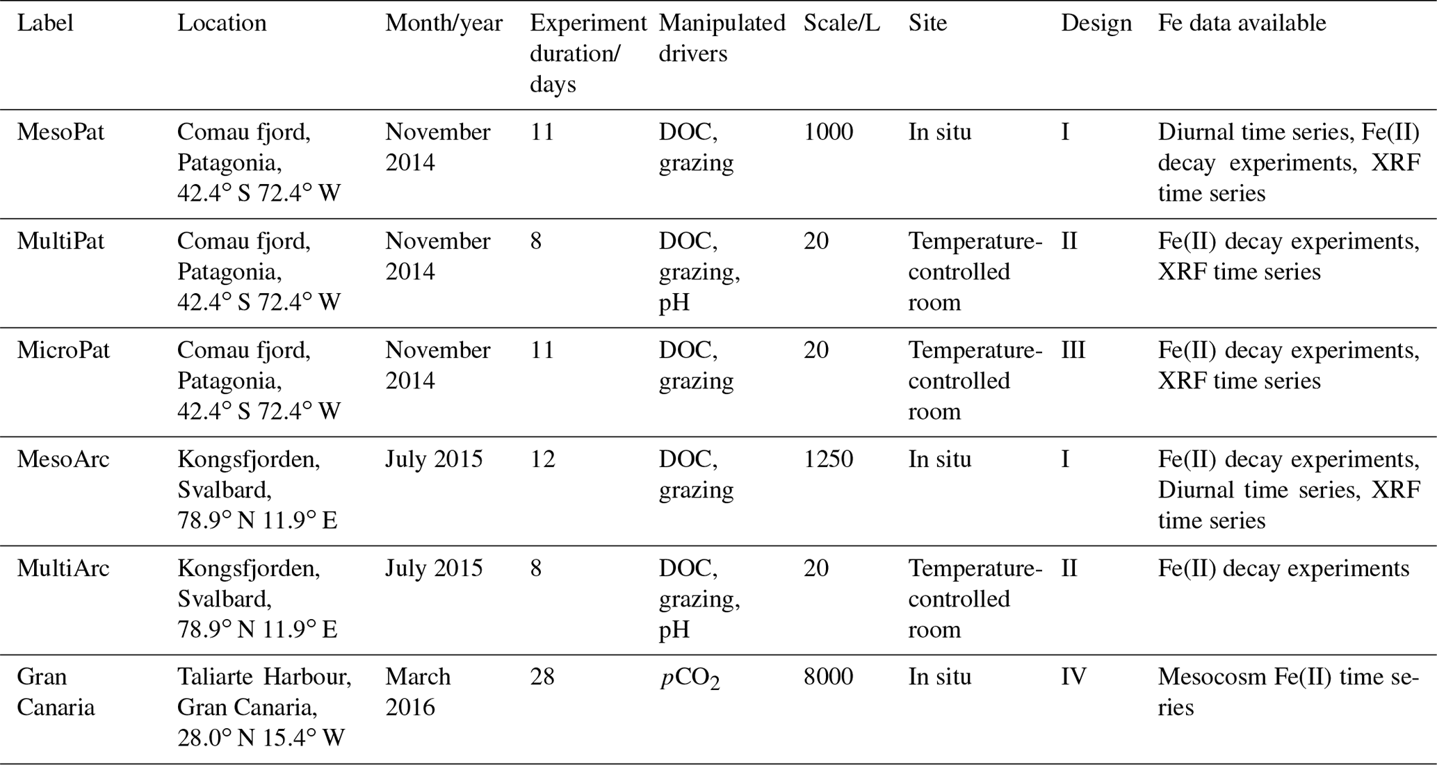
Table 2Experiment details for each experiment. “HDPE”: high-density polyethylene. Measured values are reported ± standard deviations.

2.1 Microcosm (MicroPat) and multistressor (MultiPat/MultiArc) setup and sampling
MicroPat, a 10-treatment microcosm mirroring the MesoPat mesocosm (treatment design as per MesoPat, but with six 20 L containers per treatment rather than a single HDPE tank) and two 16-treatment multistressor experiments (MultiPat/MultiArc) were conducted using artificial lighting in temperature-controlled rooms (Table 1). Coastal seawater, filtered through nylon mesh, was used to fill 20 L HDPE collapsible containers. The 20 L containers were arranged on custom-made racks with a light intensity of 80 µmol quanta m−2 s−1, approximating that at ∼3 m depth. Lamps (Phillips, MASTER TL-D 90 De Luxe 36W/965 tubes) were selected to match the solar spectrum as closely as possible. A diurnal light regime representing spring/summer light conditions at each field site was used (Table 2) and the tanks were agitated daily and after any additions (e.g. glucose, acid, or macronutrient solutions) in order to ensure a homogeneous distribution of dissolved components. In all 20 L scale experiments, macronutrients were added daily. One 20 L container from each treatment set was emptied for sampling each sample day.
The experimental matrix used for the MultiPat/MultiArc experiments duplicated the MesoPat/MesoArc design, with an additional pH manipulation: ambient and low pH. The pH of “low” pH treatments was adjusted by a single addition of HCl (trace metal grade) on day 0 only with pH measured prior to and after the addition (Table 2). Sample water from 20 L collapsible containers was extracted using a plastic syringe and silicon tubing which was mounted through the lid of each collapsible container. Throughout, where changes in Meso/Micro/Multi experiments are plotted against time, “day 0” is defined as the day the experimental gradient (zooplankton, DOC, pH, pCO2) was imposed. Time prior to day 0 was intentionally introduced during some experiments to allow water to equilibrate with ambient physical conditions after mesocosm filling. Fe(II) concentration varies on diurnal timescales, and thus during each experiment where a time series of Fe(II) or DFe concentration was measured, sample collection and analysis occurred at the same time each day.
2.2 Chemical analysis
2.2.1 Trace elements
Trace metal clean low-density polyethylene (LDPE, Nalgene) bottles were prepared via a three-stage washing procedure (1 d in detergent, 1 week in 1.2 M HCl, 1 week in 1.2 M double-distilled HNO3) and then stored empty and double bagged until use. Total dissolvable Fe (TdFe) samples were collected without filtration in trace metal clean 125 mL LDPE bottles. Dissolved Fe (DFe) samples were collected in 0.5 or 1 L trace metal clean LDPE bottles and then filtered through acid-rinsed 0.2 µm filters (PTFE, Millipore) using a peristaltic pump (Minipuls 3, Gilson) into trace metal clean 125 mL LDPE bottles within 4 h of sample collection. TdFe and DFe samples were then acidified to pH < 2.0 by the addition of HCl (150 µL, UpA grade, Romil) and stored for 6 months prior to analysis. Samples were then diluted using 1 M distilled HNO3 (SpA grade, Romil, distilled using a sub-boiling PFA distillation system, DST-1000, Savillex) and subsequently analysed by high-resolution inductively coupled plasma-mass spectrometry (HR-ICP-MS, ELEMENT XR, Thermo Fisher Scientific) with calibration by standard addition. To verify the accuracy of Fe measurements, the Certified Reference Materials NASS-7 and CASS-6 were analysed following the same dilution procedure with the measured Fe concentration, in close agreement with certified values (6.21±0.77 nM certified 6.29±0.47 nM and 26.6±0.71 nM certified 27.9±2.1 nM). The analytical blank was 0.13 nM Fe. The field blank (de-ionized, MilliQ, water handled, and filtered as if a sample in the field) was ∼0.5 nM and varied slightly between field experiments, yet was always <16 % of DFe concentration.
Fe(II) samples (unfiltered) were collected in trace metal clean translucent 50 or 125 mL LDPE bottles and analysed via flow injection analysis (FIA) using luminol chemiluminescence without preconcentration (Croot and Laan, 2002), exactly as per Hopwood et al. (2017). Fe(II) samples during the MesoPat/MesoArc/MicroPat/MultiPat/MultiArc experiments were analysed immediately after sub-sampling from each individual mesocosm/microcosm/multistressor container. In Gran Canaria the warmer seawater temperature and distance between the experiment location and laboratory precluded immediate analysis. Therefore, prior to sampling, 10 µL 6 M HCl (Hiperpur-Plus) was added to the LDPE bottles in order to maintain the sampled seawater at pH 6 and thus minimize oxidation of Fe(II) between sample collection and analysis. For Gran Canaria only, opaque LDPE bottles were used to prevent further photochemical formation of Fe(II). The pH modification is outlined in detail by Hansard and Landing (2009) and is not thought to significantly affect in situ Fe(II) concentrations during the short time period between collection and analysis. Fe(II) was then quantified within 2 h of sample collection. In all cases Fe(II) was calibrated by standard additions (normally from 0.1 to 2 nM) using 100 or 600 µM stock solutions. Stock solutions were prepared from ammonium Fe(II) sulfate hexahydrate (Sigma-Aldrich), acidified with 0.01 M HCl, and stored in the dark. A diluted Fe(II) stock solution (1–2 µM) was prepared daily. The detection limit varied slightly between FIA runs from 90 pM (Gran Canaria) to 200 pM (Arc/Pat experiments).
Wavelength dispersive X-ray fluorescence (WDXRF) was conducted on triplicates of particulate samples collected by filtering 500 mL of seawater through 0.6 µm polycarbonate filters. After air-drying overnight, samples were stored in PetriSlide boxes at room temperature until analysis at the University of Bergen (Norway). Analysis via WDXRF spectroscopy was exactly as described by Paulino et al. (2013) using an S4 Pioneer (Bruker-AXS, Karlsruhe, Germany).
2.2.2 Macronutrients and chlorophyll a
Dissolved macronutrient concentrations (nitrate, phosphate, silicic acid; filtered at 0.45 µm) were measured spectrophotometrically the same day as sample collection (Hansen and Koroleff, 2007). Nutrient detection limits inevitably varied slightly between the different mesocosm/microcosm/multistressor experiments; however, this does not adversely affect the discussion of the results herein. Chlorophyll a was measured by fluorometry as per Welschmeyer (1994).
2.2.3 Carbonate chemistry
pH (except where stated otherwise, “pH” refers to the total scale reported at 25 ∘C) was measured during the Gran Canaria mesocosm using the spectrophotometric technique of Clayton and Byrne (1993) with m-cresol purple in an automated Sensorlab SP101-SM system and a 25 ∘C-thermostatted 1 cm flow cell exactly as per González-Dávila et al. (2016). pH during MesoPat/MicroPat/MultiPat was measured similarly as per Gran Canaria using m-cresol. During MesoArc/MultiArc pH was measured spectrophotometrically as per Reggiani et al. (2016). For the calculation of Fe(II) oxidation rate constants as per Santana-Casiano et al. (2005), pHfree was calculated from measured pH using the sulfate dissociation constants derived from Dickson (1990) using CO2SYS (van Heuven et al., 2011).
2.3 In situ biogeochemical parameters
Fe(II) concentrations and other key biogeochemical parameters were measured in ambient surface (∼10–20 cm depth) water at all three experiment locations: Comau fjord for Meso/Micro/MultiPat (Patagonia, November 2014), Kongsfjorden for Meso/MultiArc (Svalbard, June 2015), and Taliarte (Gran Canaria, March 2016). FIA apparatus was assembled in waterproof boxes on floating jetties. A 3 m PTFE sample line was then positioned to float approximately 1 m away from the jetty with seawater continuously pumped into the FIA using a peristaltic pump (MiniPuls 3, Gilson). The time delay between water inflow into the PTFE line and sample analysis was 60–120 s. Complementary chemical parameters (TdFe, DFe, DOC and pH) were determined on samples collected by hand using trace metal clean 1 L LDPE bottles. Salinity and temperature data were collected with a hand-held LF 325 conductivity meter (WTW) calibrated with KCl solution. To compare Fe(II)∕H2O2 FIA data to discrete DFe∕TdFe samples, the mean of seven FIA data points, corresponding to 14 min of sample intake and analysis time, was used.
2.4 Fe(II) decay experiments
A series of experiments was conducted during Meso/Micro/MultiPat, during Meso/MultiArc (n=79), and under laboratory conditions using filtered Atlantic seawater (n=46) to investigate the change in Fe(II) concentration when water was moved from ambient light into the dark. Fe(II) decay experiments were conducted inside the temperature-controlled rooms hosting the MultiPat/MultiArc experiments. As such, a constant temperature was maintained throughout these experiments. Sub-samples for Fe(II) analysis or decay experiments were always collected when the mesocosms had been untouched (i.e. no sampling or additions) for >12 h; thus, Fe(II) species could not plausibly have been directly perturbed by any external manipulation of the mesocosm/microcosm/multistressor experiments. After collection of unfiltered 1–2 L samples in transparent 2 L HDPE containers, the PTFE FIA sample line was placed into the sample bottle and continuous analysis for Fe(II) and H2O2 begun. After a stable chemiluminescence response was obtained (typically 2–4 min after first loading the sample), the sample bottle was moved to an Al foil-lined dark laminar flow hood and analysis continued for >1 h or until Fe(II) concentration fell below the detection limit (∼0.2 nM). The time at which the sample was moved into the dark was designated t=0. Subsamples for the determination of DFe and TdFe were retained from this time point.
Theoretical decay rate constants (k′) for these experiments were calculated using the formulation presented in Santana-Casiano et al. (2005) with measured pH, temperature, dissolved O2, and salinity as per Eq. (1), where T is temperature (K), pH is pHfree, and S is salinity (psu). O2 saturation was calculated as per Garcia and Gordon (1992) and then k′ was adjusted for measured O2 concentrations as per Eq. (2). Measured rate constants (kmeas) were derived from the gradient of ln [Fe(II)] against time for each decay experiment from at least five sequential data points (Fe(II) concentration was obtained at 2 min intervals).
Dissolved O2 was measured using an Oxyminisensor (World Precision Instruments). Salinity and temperature for each experiment were measured using a hand-held LF 325 conductivity meter (WTW). Measured decay rates were determined, assuming pseudo-first-order kinetics, from linear regression of ln [Fe(II)] for t 0–15 min. Fe(II) decay experiments under laboratory conditions used aged, filtered (0.2 µm) Atlantic water. This water was previously stored filtered in 1 m3 trace element clean HDPE containers for in excess of 1 year and maintained in the dark at experimental temperature for 3 d prior to commencing any experiment.
2.5 Quantifying the potential for Fe contamination during a mesocosm experiment
During MesoArc a “bookkeeping” exercise was conducted for the mesocosm experiment by the sub-sampling of all solutions added to the incubated seawater. Aqueous additions consisted of HCl solution (used to apply the pH gradient), macronutrient solution, glucose solution, and zooplankton. A short (1–2 h) 1 M HCl (trace metal grade) leach was applied to equipment placed within the mesocosm and also to the HDPE mesocosm containers prior to filling to provide a quantitative estimate of “leachable” Fe. Atmospheric deposition of Fe into the tanks when open was estimated by deploying open bottles of de-ionized water within the vicinity of the mesocosms for fixed time intervals of 1 h in triplicate on three occasions and recording the approximate extent of time when the mesocosm lids were removed. All additions to the MesoArc mesocosm experiment were volume weighted as per Eq. (3) using the mean (mid-experiment) mesocosm volume (Vmesocosm) and assuming that all additions were well mixed and TdFe behaved conservatively.
3.1 “Bookkeeping” Fe additions for a 1000 L mesocosm experiment (MesoArc)
In order to provide a rigorous assessment of Fe contamination during one experiment, Fe inputs were tracked in all additions to MesoArc and scaled to the mesocosm volume (initially 1200 L, declining by 15 % over the experiment duration). Volume weighting all additions (Table 3) to the MesoArc mesocosm experiment as per Eq. (3) produced a total mean concentration of 48 nM TdFe (Fig. 1). In addition to the uncertain variability arising as the mesocosms were filled, approximately 8 % (3.6 nM) of TdFe within the MesoArc experiment could be attributed to inadvertent addition (Fig. 1) over the experiment duration.

Figure 1Volume-weighted additions of TdFe to the same experimental design at three mesocosm experiments. For MesoArc all inputs to the mesocosm were explicitly quantified. For MesoPat/MesoMed the initial water mass TdFe was quantified and TdFe inputs were adjusted as if the MesoArc experiment had been exactly duplicated with only the initial water mass changed.
When MesoArc is compared to the two other mesocosms with a similar design (MesoPat and MesoMed), the TdFe inputs and the relative contribution of inadvertent TdFe addition were 66.9 nM TdFe with 4.8 % arising from inadvertent addition for MesoPat and 13.3 nM with 24 % TdFe arising from inadvertent addition for MesoMed (Fig. 1). Systematic contamination was in all cases a minor, yet measurable, source of TdFe for these inshore mesocosms. Strictly, the inadvertent input of TdFe varied between different treatments within each mesocosm experiment due to, for example, the variable volume of glucose solution used to create a DOC gradient (Table 1). However, these differences caused small or negligible changes in TdFe addition (Table 3).
Table 3Total dissolvable Fe (TdFe) additions to the MesoArc mesocosm containers associated with sources other than the initial water mass.
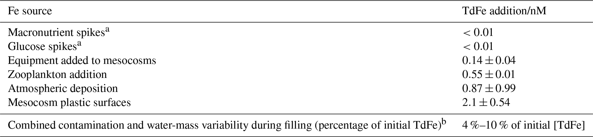
a These TdFe concentrations were measurable but negligible when scaled to the mesocosm volume. b Based on TdFe measurements at time zero from the MesoPat multistressor/microcosm and DSi measurements on experiment day 0 or day 1 from multiple mesocosms.
3.2 General trends in Fe biogeochemistry; the MesoArc and MesoPat mesocosms
Concentrations of both DFe and H2O2 (as per Hopwood et al., 2020) were measured at the highest resolution for the baseline treatments (no DOC addition, no zooplankton addition) during the mesocosm experiments. For MesoPat (Fig. 2), the initial concentration of DFe and H2O2 was estimated by using a Go-Flo bottle to sample at a depth of 10 m in the fjord (at which approximate depth the mesocosms were filled from). The apparent rise in H2O2 between day 0 and day 1 (Fig. 2) likely reflects the result of increased formation of H2O2 after pumping of water from ∼10 m depth into containers at the surface. NO3 was added daily (Table 2); hence, concentrations increased prior to the onset of a phytoplankton bloom. The decline in DFe likely reflects biological uptake and/or scavenging onto particle (>0.2 µm) or mesocosm container surfaces.
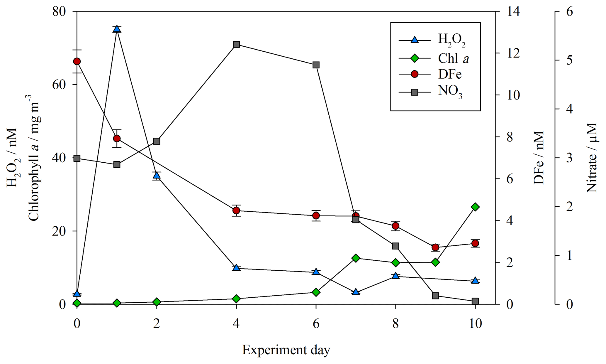
Figure 2DFe (red circles), hydrogen peroxide (H2O2, blue triangles), nitrate (NO3, grey squares), and chlorophyll a (green diamonds) for the baseline treatment (no DOC addition, no added zooplankton) during the MesoPat mesocosm.
Less frequent temporal resolution was available for treatments other than the “baseline” (no DOC/zooplankton addition) treatment, but the decline in DFe during the MesoPat mesocosm was apparent across all measurements considered together. In addition to TdFe measurements from unfiltered water samples, particulate (>0.6 µm) Fe concentrations were also determined from wavelength dispersive X-ray fluorescence. WDXRF data were normalized to phosphorus (P) in order to discuss trends in the elemental composition of particles and are thus presented as the Fe:P (mol Fe mol−1 P) ratio. The initial Fe:P ratio in particles varied between the mesocosm field sites: MesoPat 0.34±0.09 and MesoArc 0.62±0.07. A similar trend however was observed during all experiments: a general decline in Fe:P across all treatments with time. Particulate Fe:P ratios on the final day of measurements were invariably lower than the initial ratio: MesoPat 0.09±0.04, MicroPat 0.05±0.01, MultiPat 0.07±0.03, and MesoArc 0.17±0.08. All of these ratios are high compared to literature values reported for offshore stations where the ratio for cellular material ranged from 0.005 to 0.03 mol Fe mol−1 P (Twining and Baines, 2013). However, this may simply reflect elasticity in Fe:P ratios which increase under high DFe conditions (Sunda et al., 1991; Sunda and Huntsman, 1995). Alternatively, it could reflect the inclusion of a large fraction of lithogenic material, which would be expected to have a higher Fe:P ratio than biogenic material (Twining and Baines, 2013).
Particles from ambient waters outside the mesocosms were collected and analysed at the Patagonia and Svalbard field sites in order to assist in interpreting the temporal trend in Fe:P. Suspended particles from Kongsfjorden (Svalbard) exhibited a Fe:P ratio of 3.01±0.06 mol Fe mol−1 P and suspended particles in Comau fjord (Patagonia) varied more widely, with a mean ratio of 0.54±0.41 mol Fe mol−1 P. Kongsfjorden surface waters are characterized by extremely high TdFe concentrations originating from particle-rich meltwater plumes (Hop et al., 2002) and thus the 3.0 Fe:P ratio can be considered to be a lithogenic signature. After ambient water was collected for the mesocosm experiments, the steady decline in particle Fe:P ratios throughout the experiments likely resulted partially from a settling or aggregation of lithogenic material after filling of the mesocosms. At the same time, a decline in the ratio of dissolved Fe:PO4 during each experiment, due to the daily addition of PO4 and minimal addition of new Fe, may also have led to reduced Fe uptake relative to P.
3.3 Fe(II) time series (Gran Canaria)
A key focus of this work was to determine the fraction of DFe present as Fe(II). During the Gran Canaria mesocosm, a detailed time series of Fe(II) concentrations was conducted. The timing of sample collection was the same daily (14:30 UTC) in order to minimize the effect of changing light intensity over diurnal cycles on measured Fe(II) concentrations. Over the duration of the Gran Canaria mesocosm, Fe(II) concentrations fell within the range 0.10–0.75 nM (Fig. 3a). On the first measured day (day −2) Fe(II) ranged from 0.13 nM (mesocosm 7, 700 µatm pCO2) to 0.63 nM (mesocosm 6, 1450 µatm pCO2), with an overall mean (± standard deviation) concentration of 0.41±0.12 nM. From days 9 to 20 strong variations were observed between treatments. Following nutrient addition on day 18, a phytoplankton bloom was evident in chlorophyll a data from day 19 or day 20, with chlorophyll a peaking on day 21 or later (Hopwood et al., 2018). An increase in Fe(II) was then evident from days 20 to 29 under bloom and post-bloom conditions (Fig. 3b).
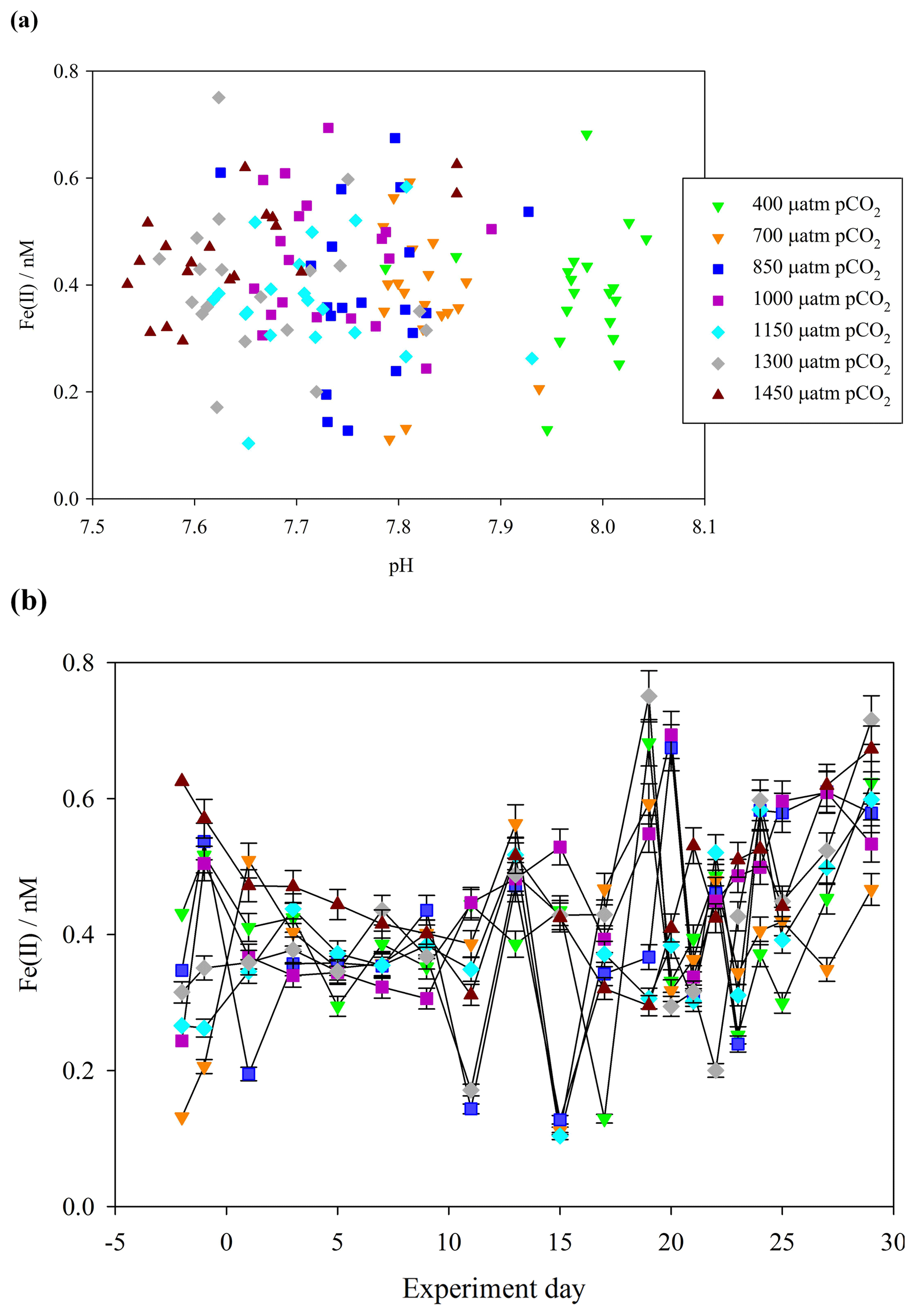
Figure 3(a) Fe(II) concentrations (unfiltered) during the Gran Canaria mesocosm plotted against measured mesocosm pH (b) Fe(II) concentrations over the duration of the Gran Canaria mesocosm experiment. The 550 µatm pCO2 mesocosm was discontinued after leakage and exchange with surrounding seawater occurred on experiment day 3, and so no data are shown.
Contrasting days 1 and 29, Fe(II) in all of the mesocosms except the 700 µatm pCO2 treatment experienced a measurable increase in Fe(II) concentration (+0.4, +0.4, +0.2, +0.2, +0.2, 0.0, and +0.3 nM). The 700 µatm pCO2 treatment was also anomalous with respect to slow post-bloom nitrate drawdown and elevated H2O2 concentration (100 nM H2O2 greater than other treatments under post-bloom conditions, Hopwood et al., 2018). Overall, despite the large gradient in pCO2 (400–1450 µatm and a corresponding measured pH range of 8.1–7.7), Fe(II) showed no significant correlation with pH (Pearson product moment correlation p0.32) (Fig. 3a).
3.4 Fe(II) decay experiments (Meso/Micro/MultiPat and Meso/MultiArc)
In a companion text presenting H2O2 results from the same series of experiments (Hopwood et al., 2020), a series of experiments in the Mediterranean (MesoMed/MultiMed) is also included. During these Mediterranean experiments however the rapid oxidation rate of Fe(II) precluded the determination of Fe(II) concentrations. Fe(II) concentrations were universally <0.2 nM (i.e. below detection), and thus no Fe(II) results from the “Med” experiments are presented herein. During the MesoArc and MesoPat experiments, a series of decay experiments was conducted to investigate the stability of in situ Fe(II) concentrations. The 79 time points at the start of these experiments were made before water was moved from ambient lighting into the dark and can be considered in situ Fe(II) concentrations. Across the complete dataset, the properties known to affect the rate of Fe(II) oxidation in seawater varied over relatively large ranges for the various experiments: temperature 4.0–18 ∘C, salinity 22.7–33.8, pH 7.46–8.44, 315–449 µM O2, and 1–79 nM H2O2 (see Supplement). Initial Fe(II) concentrations ranged from 0.3 to 16 nM. Generally a decline in Fe(II) was observed immediately after transferring this sampled water to a dark box, yet this was not always the case. The Fe(II) concentration more often than not remained measurable (>0.2 nM) for the entire duration of the decay experiment. One hour after the transfer of water from ambient conditions into the dark, Fe(II) was below detection on only 2 out of 79 occasions, and on average 55 % of the initial Fe(II) concentration at t=0 remained.
In order to account for the many physio-chemical parameters that affect Fe(II) oxidation rates, theoretical pseudo-first-order rate constants (k′) were calculated for each decay experiment assuming pseudo-first-order kinetics (correlation coefficients are noted for each linear regression – Supplement). The rate constant, k (Eq. 1), thus accounts for the major effect of variations between experiments of salinity, temperature, pH, and O2 in a single constant (Fig. 4). Before comparing kmeas and k, an estimate of the uncertainty should also be made as differences between the two values may arise due to the relatively large combined error from propagating the uncertainty in , and in analytical error on Fe(II) measurements. The accuracy of Fe(II) measurements is challenging to quantify for a transient species with no appropriate reference material. In this case, the exact Fe(II) detection method used here was previously compared to another variation of the luminol chemiluminescence method (with pre-concentration, Bowie et al., 2002), and kmeas was determined with ±20 % difference between the two methods. The uncertainty in kmeas is therefore assumed to be ±20 % rather than the generally smaller uncertainty that can be calculated from linear regression of ln [Fe(II)]. The uncertainty in calculated k was assessed by calculating the change resulting from the estimated uncertainty in measured salinity (±0.1), temperature (±0.5 ∘C), pHfree (±0.05), and O2 (±10 µM). The combined uncertainty is ±35 % for k. Reduced uncertainties are possible with closed thermostat systems where the uncertainty in all physical/chemical parameters () would be reduced; however, our objective here was to measure the decay rates of in situ Fe(II) concentrations, and thus the first priority was to commence measurements after sub-sampling rather than to stabilize physical/chemical conditions.
In order to further understand the cause of any systematic discrepancies in the dataset between measured kmeas and calculated k, an additional set of experiments was conducted using aged, filtered Atlantic seawater (Fig. 4). The background concentration of Fe(II) in this water was below detection (<0.2 nM) and the initial DFe concentration relatively low (0.98±0.39 nM). In a series of 46 decay experiments, Fe(II) spikes of 2–8 nM were added and then the decay in the dark monitored as per the Meso/Micro/Multi Arc/Pat in situ experiments.
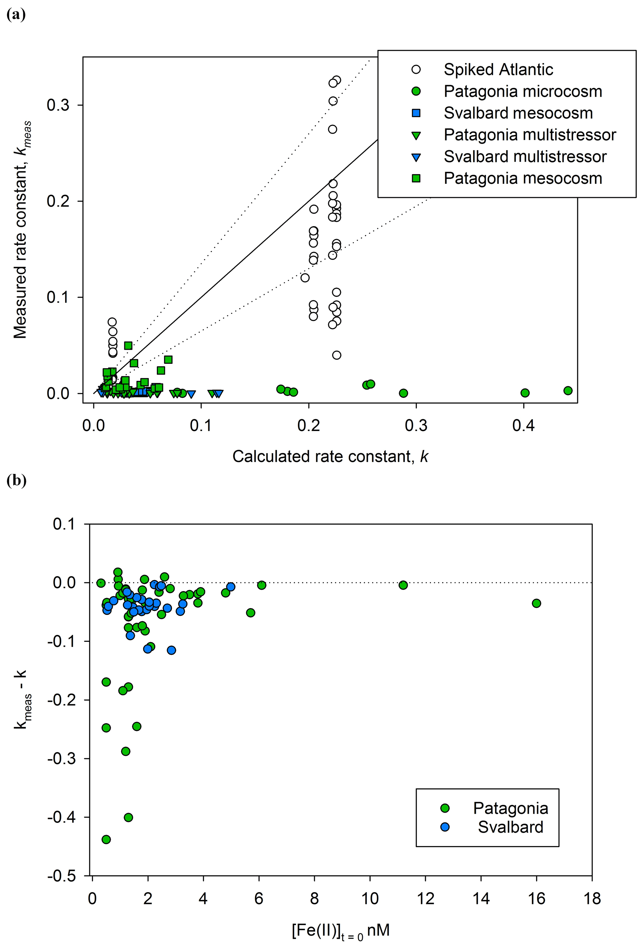
Figure 4A comparison of kmeas and calculated k (both M−1 min−1) for Fe(II) decay experiments. (a) Rate constants for Fe(II) decay experiments from Meso/Micro/MultiPat (green) and Meso/MultiArc (blue) and spikes to aged Atlantic seawater (colourless). (b) The difference between observed and calculated values of k () is shown against initial Fe(II) concentration.
4.1 Assessing the extent of Fe contamination within a mesocosm experiment (MesoArc)
Assembling and maintaining mesocosm-scale experiments under trace-element clean conditions is a logistically challenging exercise (e.g. Guieu et al., 2010) and thus it was desirable to conduct a thorough assessment of the extent to which Fe concentrations were subject to inadvertent increases during at least one experiment. All of the incubation experiments herein were conducted using coastal or near-shore waters. This is reflected in the low salinities of the MesoPat (27.5–28.0) and MesoArc (33.7–33.8) mesocosms. Both of these field sites were fjords with high freshwater input. Comau fjord (Patagonia, MesoPat) is situated in a region with high annual rainfall and receives discharge from rivers including the River Vodudahue. Kongsfjorden (Svalbard, MesoArc) receives freshwater discharge from numerous meltwater-fed streams and marine-terminating glaciers in addition to melting ice. Correspondingly high DFe and TdFe concentrations were thereby found in surface waters, universally >4 nM DFe. The Gran Canaria (initial S37.0) mesocosm cannot be considered to have had a coastal low-salinity signature from freshwater outflows, but was still conducted using near-shore waters which would generally be expected to contain higher Fe concentrations than offshore waters due to sedimentary sources of Fe (see, for example, Croot and Hunter, 2000). Despite the inshore basis of MesoArc, Fe contamination was a small, but significant, fraction of the TdFe added to the starting water (8 %, 3.6 nM, Fig. 1). It is not anticipated that this small TdFe addition will have had any adverse effect on the Fe redox chemistry results presented herein for the Meso/Micro/Multi Arc/Pat experiments.
4.2 Fe speciation within the mesocosms
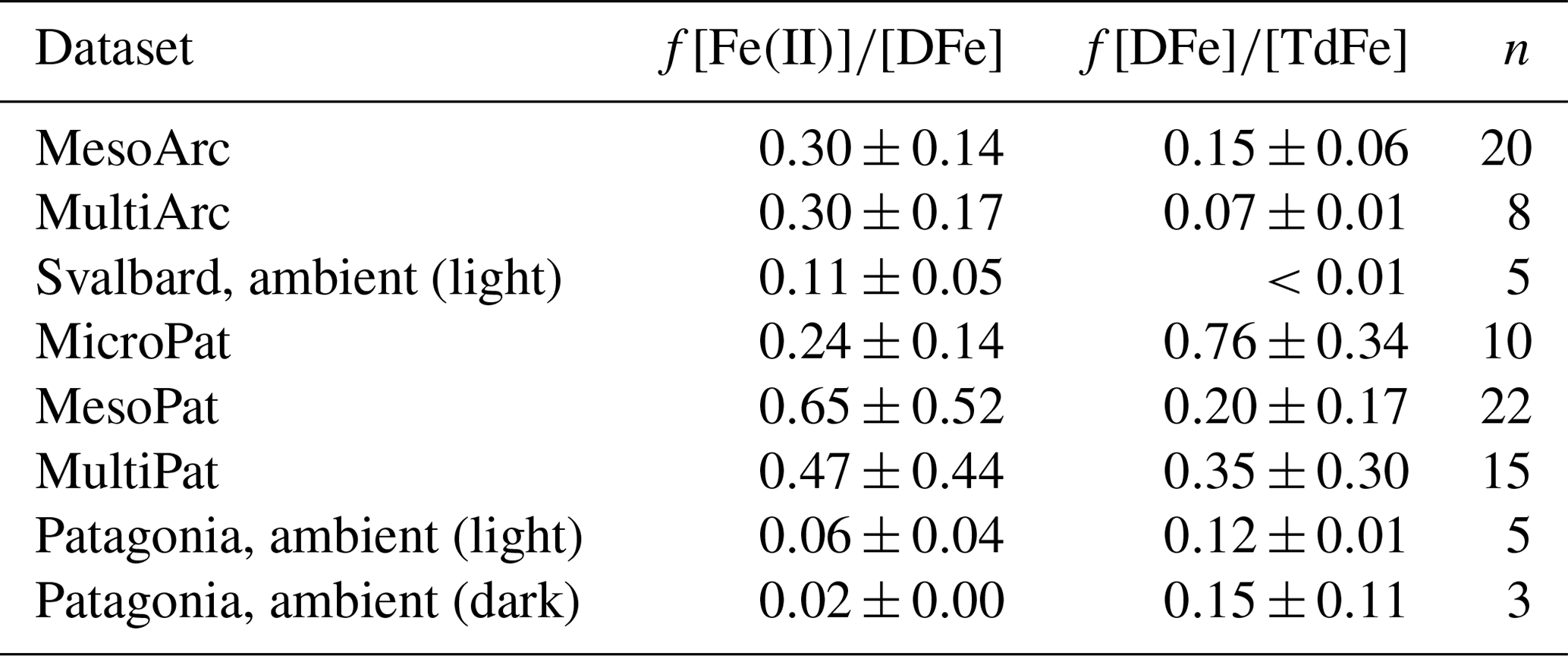
Throughout all of the Meso/Micro/Multi Arc/Pat experiments, Fe(II) consistently constituted a large fraction of DFe (Table 4). The presence of 24 %–65 % of DFe in mesocosms as Fe(II) is not unexpected, as the photoreduction of Fe(III) species by sunlight is well characterized (Wells et al., 1991; Barbeau, 2006). Yet it also raises questions about how Fe speciation is modelled in these waters. DFe in the ocean is widely assumed to be characterized as “99 % complexed by organic species” (Gledhill and Buck, 2012) on the basis of extensive research using voltammetric titrations to determine the strength and concentration of Fe-binding ligands (Van Den Berg, 1995; Rue and Bruland, 1995). Yet these approaches exclusively measure Fe(III)-L species (Gledhill and Buck, 2012).
Table 4Fraction of dissolved Fe concentration ([DFe]) present as Fe(II) and fraction of total dissolvable Fe concentration ([TdFe]) present as DFe. n, number of data points. ND, not determined. All values are mean ± standard deviation.
Here we should note that the method utilized during these incubation and diurnal experiments, flow injection analysis with a PTFE line inserted directly into the experiment water, is relatively well suited for establishing the in situ concentration of Fe(II) (O'Sullivan et al., 1991). Such an experimental setup ensures no unnecessary delay is introduced between the collection and analysis of a sample. When using an opaque sampler, such as a Go-Flo bottle typically deployed at sea for collection of trace element samples (Cutter and Bruland, 2012), the collection process inevitably displaces near-surface water from its ambient light conditions for a time period that constitutes >1 half-life of Fe(II) in warm, oxic seawater. Measured near-surface Fe(II) concentrations on samples from a rosette system would therefore always be expected to under-estimate in situ near-surface Fe(II) concentrations (O'Sullivan et al., 1991).
Fe(II) concentration was also quantified in ambient waters adjacent to the mesocosms and found to constitute a lower fraction of DFe (2 %–11 %). Most of the decay experiments, from which initial Fe(II) concentrations are reported (Table 4), were conducted at the end of Meso/Micro/Multi experiments, and thus it is not possible to assess the development of Fe(II) stability throughout a phytoplankton bloom. Nevertheless, the high fraction of DFe present as Fe(II) in these experiments (Table 4) relative to that observed in ambient waters is consistent with the increase in Fe(II) concentrations observed in Gran Canaria after the initiation of the phytoplankton bloom (day 19 onwards, Fig. 3b). The Meso/Micro/Multi Arc/Pat experiments had macronutrient additions daily, whereas the Gran Canaria experiment had macronutrient addition only on day 18. The conditions within the Meso/Micro/Multi Arc/Pat experiments during the time period in which decay experiments were conducted were therefore typical of those during, or shortly after, a phytoplankton bloom. Whilst chlorophyll a was not quantified for ambient waters, for which Fe(II) data are reported (Table 4), sampling in Svalbard (MesoArc, July 2015) and Patagonia (MesoPat, November 2014) occurred during relatively low-productivity phases of the annual cycle in primary production at these field sites (Hop et al., 2002; Iriarte et al., 2013). The ambient concentrations of Fe(II) measured at the mesocosm experiment field sites are therefore not necessarily directly comparable to Fe(II) concentrations measured after nutrient addition in the corresponding mesocosm experiments.
4.3 Fe(II) decay experiments
Fe(II) oxidation rates are relatively well constrained in seawater with varying temperature, salinity, pH, H2O2, and O2 concentrations from extensive series of experiments where the change in concentration of an Fe(II) spike was monitored with time and the rate constants for oxidation with O2 and H2O2 were then derived from first-order kinetics (Millero et al., 1987; King et al., 1995). Whilst dissolved O2 is the dominant oxidizing agent for Fe(II), H2O2 is also of importance as an Fe(II) oxidizing agent in surface seawater (Millero and Sotolongo, 1989; King and Farlow, 2000; González-Davila et al., 2005). The unusually low concentration of H2O2 within the Meso/Micro/Multi Arc/Pat experiments due to the enclosed HDPE mesocosm design and/or synthetic lighting (Hopwood et al., 2020) was therefore fortunate from a mechanistic perspective as it allows the simplification that O2 was the only major oxidizing agent. The much lower H2O2 concentrations (1–79 nM) present, compared to ambient surface waters, throughout the Meso/Micro/Multi Arc/Pat experiments should mean that Fe(II) decay rates during these experiments more closely match the oxidation rate constants used to derive Eq. (1) (which were derived for low-H2O2 conditions).
The decay experiments reported here still however differ in two critical respects from controlled oxidation rate experiments used to derive rate constants. First, the speciation of Fe(II) may differ. It is debatable to what extent Fe(II)-L species, analogous to Fe(III)-L species, exist in surface marine waters due to the absence of reliable techniques to probe Fe(II)-organic speciation (Statham et al., 2012). Yet there is consistent evidence that organic material affects Fe(II) oxidation rates (see below). Second, these decay experiments measure the change in Fe(II) concentration between light and dark conditions and not specifically the oxidation rate. If photochemical Fe(II) production was the sole Fe(II) source, and oxidation of Fe(II) via H2O2 and O2 were the only Fe(II) sink, then the decay rate measured here would approximate the oxidation rate determined under controlled laboratory conditions. However, there are possible biological sources of Fe(II) (Sato et al., 2007; Nuester et al., 2014), the possibility of biological uptake of Fe(II) (Shaked and Lis, 2012), and cross-reactivity with other reactive trace species (e.g. reactive oxygen species and Cu, Rijkenberg et al., 2006; Croot and Heller, 2012) to consider. These complexities make Fe(II) more challenging to model in natural waters compared to controlled conditions. This is especially the case at the low Fe(II) concentrations relevant to the surface ocean, where Fe(II) concentrations range from below detection up to ∼1 nM (Gledhill and Van Den Berg, 1995; Hansard et al., 2009; Sarthou et al., 2011).
Contrasting k with kmeas during Fe(II) decay experiments (Fig. 4), it is immediately apparent that the Fe(II) present within Meso/Micro/Multi Arc/Pat experiments was generally much more stable than would be predicted for an equivalent inorganic spike of Fe(II) added to water with the same physical/chemical properties; i.e. in most cases kmeas<k. Three plausible hypotheses can be conceived for the offset.
- i.
The measured rates here refer to relatively low initial Fe(II) concentrations (0.3–16 nM) compared to the concentrations at which rate constants have been derived (typically ∼20–200 nM), and the difference arises simply because the rate constants are not calibrated for low nanomolar starting concentrations.
- ii.
There is “dark” production of Fe(II) in the experiments; i.e. ongoing formation of Fe(II) counteracts the first-order decay of Fe(II) via oxidation.
- iii.
The speciation of Fe(II) in seawater is more stable with respect to oxidation than the species for which the rate constants are calculated.
For the series of experiments using spikes of Fe(II) in Atlantic seawater, kmeas is consistently closer to k than for any in situ experiments (Fig. 4a). Nevertheless, some data points for spiked Atlantic seawater still fall outside the ±35 % uncertainty boundary. As the spiked experiments closely matched the initial Fe(II) concentrations in the in situ decay experiments, the higher Fe(II) concentrations generally used to establish the rate of Fe(II) decay in laboratory experiments cannot be the main explanation for a discrepancy between kmeas and k. Furthermore, differences in the formulation of k′ between studies are relatively minor (Millero et al., 1987; King et al., 1995; Santana-Casiano et al., 2005).
Calculating the difference between calculated and measured k (Δk), it is evident that the largest differences were associated with the lowest initial Fe(II) concentrations (Fig. 4b). This is consistent with both hypothesis II and hypothesis III. Assuming that the dominant source of Fe(II) is photochemistry, the effects of both a secondary “dark” Fe(II) source and a limited fraction of Fe(II) existing in a more stable form with respect to oxidation would be most evident at the lowest initial Fe(II) concentration. Sources of Fe(II) other than photochemistry are plausible and may include, for example, zooplankton grazing due to the reduced pH and O2 within organisms (Tang et al., 2011; Nuester et al., 2014). Mesozooplankton addition was one of the three experimental variables manipulated during the Arctic/Patagonia experiments. However, no clear trend was evident with respect to Δk and the zooplankton addition status of the experiments. Mean for the high/low zooplankton treatments over all the experiments were 4.66±5.79 and 4.08±5.63, respectively. A dependency of Δk on the initial Fe(II) concentration (Fig. 4b), with [Fe(II)]t=0 likely very sensitive to multiple experimental factors such as the time of day that the sample was collected and the exact time delay between sample collection and the first time point for each Fe(II) decay experiment, would however make determining the relative importance of any other underlying causes challenging. In order to gain further insight into the potential role of zooplankton in Fe(II) release under dark conditions, a series of incubations was conducted with addition of the copepod Calanus finmarchichus to cultures of the diatom Skeletonema costatum (Hopwood et al., 2020). No changes in extracellular Fe(II) or H2O2 concentrations were evident across a gradient of copepods from 0 to 10 L−1. Whilst this suggests the role of high/low zooplankton treatments was minimal in short-term changes to ambient Fe(II) concentrations, the potential release of Fe(II) by zooplankton may of course be species-specific: different results may have been obtained with different zooplankton–prey combinations.
The high magnitude of Δk in some cases at low initial Fe(II) concentrations (Fig. 4) is consistent with the theory that Fe(II)-binding ligands are responsible for the observed stability of Fe(II) in some natural waters (Roy and Wells, 2011; Statham et al., 2012). The Fe(II)-binding capacity of any ligands present in a specific sample would be expected to become saturated as Fe(II) concentrations increased. The effect of Fe(II) ligands on the oxidation rate of an added Fe(II) spike would therefore become less evident as Fe(II) concentration increased because the fraction of Fe(II) present as Fe(II)-L species would decline; i.e. Δk would approach zero. This has an important methodological implication. The effect of cellular exudates, or natural organic material extracts, on Fe(II) oxidation rate is more often than not tested by adding reasonably high nanomolar Fe(II) spikes to solution and then following the Fe(II) decay with time (see, for example, Lee et al., 2017). By raising the initial Fe(II) concentration, such an approach may however systematically under-estimate the effect of organic material on Fe(II) stability at in situ Fe(II) concentrations.
The effect of organic material on Fe(II) is difficult to generalize as organic compounds can accelerate, retard, or have no apparent effect on Fe(II) oxidation rates via O2 (Santana-Casiano et al., 2000). However, there are now sufficient studies of Fe(II) behaviour to distinguish between the broad effects of allochthonous and autochthonous material. Extracts from the green algae Dunaliella tertiolecta (González et al., 2014), cyanobacteria Synechococcus (Samperio-Ramos et al., 2018b) and Microcystis aeruginosa (Lee et al., 2017), coccolithophore Emiliania huxleyi (Samperio-Ramos et al., 2018a), and diatoms Chaetoceros radicans (Lee et al., 2017) and Phaeodactylum tricornutum (Santana-Casiano et al., 2014) have all been found to retard Fe(II) oxidation rates. Furthermore, the effect of cellular exudates on the reaction constant appears to scale with increasing total organic carbon (Samperio-Ramos et al., 2018b). In contrast to the stabilization apparent in some cellular exudates, allochthonous material generally, although not universally, has the opposite effect, with an acceleration of Fe(II) oxidation rates reported both in coastal environments (Lee et al., 2017) and using terrestrially derived organic leachates (Rose and Waite, 2003). The generally positive effects of cellular exudates on Fe(II) stability with respect to oxidation determined in single-species studies is consistent with the stability of Fe(II) observed in almost all experiments here (Fig. 4), and this suggests that microbial cellular exudates are indeed a stabilizing influence on Fe(II) concentrations at a broad scale in coastal marine environments. Stabilization of Fe(II) by freshly produced exudates could explain the sustained increase in Fe(II) concentrations across all pCO2 treatments under post-bloom conditions in Gran Canaria (Fig. 3b) and the high fraction of DFe present as Fe(II) during all Meso/Micro/Multi Arc/Pat experiments (Table 4).
Apart from the influence of organic Fe(II) ligands on Fe(II) stability arising from the slower oxidation rates of some organically complexed Fe(II) species, Fe(II)-binding organics may also have a role in the generation of superoxide (), which is speculated to be a dominant mechanism for the formation of Fe(II) in the dark (Rose, 2012). Experiments with 65–130 nM of protoporphyrin IX demonstrated increased formation of Fe(II) in the dark with both increasing porphyrin concentration and increasing irradiation of seawater prior to the onset of darkness (Rijkenberg et al., 2006). Whilst the rates of this process are challenging to investigate at the sub-nanomolar porphyrin and Fe(II) concentrations expected in the ocean's dark interior, the dark formation of Fe(II) mediated by reactive oxygen species' interactions with Fe(II)-organic complexes could potentially be important in both the diurnal cycling of Fe in the surface ocean and the non-photochemical formation of Fe(II) in the dark of the ocean's interior (Rose, 2012). From a mechanistic perspective, it is challenging to establish definitively from the experiments herein whether apparent Fe(II) stability arises from reduced oxidation rates due to Fe(II) complexation or dark Fe(II) formation via a mechanism, such as that proposed for superoxide, which involves Fe(II)-organic complexes. Both hypotheses are consistent with field observations, and it is also possible that both processes operate in parallel.
The existence of a high fraction (24 %–65 %) of DFe as Fe(II) during mesocosm experiments and the apparent stability of low concentrations of Fe(II) suggest that the classic characterization of “99 % of dissolved Fe existing as Fe(III)-L complexes” (Gledhill and Buck, 2012) is inadequate for describing DFe speciation in coastal surface waters. Fe(III)-ligand complexes may overwhelmingly dominate Fe speciation in the ocean as a whole, but in surface coastal waters a dynamic redox cycle operates, maintaining considerable concentrations of Fe(II) in solution. The stabilizing effects on Fe(II) with respect to oxidation reported here were strongest at low (<2 nM) Fe(II) concentrations, suggesting that the Fe(II) stabilization mechanism is caused by a process akin to complexation where the magnitude of the effect is capped by a factor other than physical conditions.
Exudates stabilizing Fe(II) may be a poorly characterized component of the aptly named “ferrous wheel” (Kirchman, 1996; Strzepek et al., 2005) and contribute to the efficient recycling of DFe within marine surface waters. Irrespective of whether Fe(II) is more or less bioavailable relative to Fe(III), the formation of Fe(II) is a mechanism for increasing DFe and thus increasing DFe availability to biota. Mechanisms such as the stabilization of Fe(II) by cellular exudates during and after phytoplankton blooms may therefore facilitate DFe uptake to a greater extent than would be possible in the absence of Fe-redox cycling. Both Fe(III) and Fe(II) speciation and concentration must therefore be defined in order to understand the role of Fe as a driver of marine primary production.
Full datasets for the mesocosm and microcosm experiments are available from https://doi.pangaea.de/10.1594/PANGAEA.911130 (Sanchez et al., 2020).
The supplement related to this article is available online at: https://doi.org/10.5194/bg-17-1327-2020-supplement.
All the authors contributed to the design of the study and the interpretation of data. MJH, CSG, JGU, NS, ØL, and TMT conducted analytical work. MJH coordinated the writing of the manuscript with input from the other authors.
The authors declare that they have no conflict of interest.
The Ocean Certain and KOSMOS/PLOCAN teams assisting with all aspects of experiment logistics and organization are thanked for their efforts. Labview software for operating the Fe(II) FIA system was designed by Peter Croot, Maija Heller, Craig Neill and Whitney King.
This research has been supported by the European Commission (OCEAN-CERTAIN (grant no. 603773)), the Deutsche Forschungsgemeinschaft (Collaborative Research Centre 754 Climate-Biogeochemistry Interactions in the Tropical Ocean), and the Ministerio de Economía y Competitividad (EACFe project (grant no. CTM2014-52342-P)).
The article processing charges for this open-access
publication were covered by a Research
Centre of the Helmholtz Association.
This paper was edited by Caroline Slomp and Marilaure Grégoire and reviewed by Andrew Rose and one anonymous referee.
Barbeau, K.: Photochemistry of organic iron(III) complexing ligands in oceanic systems, Photochem. Photobiol., 82, 1505–1516, https://doi.org/10.1562/2006-06-16-IR-935, 2006.
Boukhalfa, H. and Crumbliss, A. L.: Chemical aspects of siderophore mediated iron transport, Biometals, 15, 325–339, https://doi.org/10.1023/a:1020218608266, 2002.
Bowie, A. R., Achterberg, E. P., Sedwick, P. N., Ussher, S., and Worsfold, P. J.: Real-time monitoring of picomolar concentrations of iron(II) in marine waters using automated flow injection-chemiluminescence instrumentation, Environ. Sci. Technol., 36, 4600–4607, https://doi.org/10.1021/es020045v, 2002.
Boyd, P. W., Strzepek, R., Fu, F., and Hutchins, D. A.: Environmental control of open-ocean phytoplankton groups: Now and in the future, Limnol. Oceanogr., 55, 1353–1376, https://doi.org/10.4319/lo.2010.55.3.1353, 2010.
Breitbarth, E., Gelting, J., Walve, J., Hoffmann, L. J., Turner, D. R., Hassellöv, M., and Ingri, J.: Dissolved iron (II) in the Baltic Sea surface water and implications for cyanobacterial bloom development, Biogeosciences, 6, 2397–2420, https://doi.org/10.5194/bg-6-2397-2009, 2009.
Chever, F., Rouxel, O. J., Croot, P. L., Ponzevera, E., Wuttig, K., and Auro, M.: Total dissolvable and dissolved iron isotopes in the water column of the Peru upwelling regime, Geochim. Cosmochim. Ac., 162, 66–82, https://doi.org/10.1016/j.gca.2015.04.031, 2015.
Clayton, T. D. and Byrne, R. H.: Spectrophotometric seawater pH measurements: total hydrogen ion concentration scale calibration of m-cresol purple and at-sea results, Deep-Sea Res. Pt. I, 40, 2115–2129, https://doi.org/10.1016/0967-0637(93)90048-8, 1993.
Conway, T. M. and John, S. G.: Quantification of dissolved iron sources to the North Atlantic Ocean, Nature, 511, 212–215, https://doi.org/10.1038/nature13482, 2014.
Croot, P. and Heller, M.: The Importance of Kinetics and Redox in the Biogeochemical Cycling of Iron in the Surface Ocean, Front. Microbiol., 3, 219, https://doi.org/10.3389/fmicb.2012.00219, 2012.
Croot, P. L. and Hunter, K. A.: Labile forms of iron in coastal seawater: Otago Harbour, New Zealand, Mar. Freshwater Res., 51, 193–203, https://doi.org/10.1071/Mf98122, 2000.
Croot, P. L. and Laan, P.: Continuous shipboard determination of Fe(II) in polar waters using flow injection analysis with chemiluminescence detection, Anal. Chim. Acta, 466, 261–273, https://doi.org/10.1021/ac015547q, 2002.
Croot, P. L., Bowie, A. R., Frew, R. D., Maldonado, M. T., Hall, J. A., Safi, K. A., La Roche, J., Boyd, P. W., and Law, C. S.: Retention of dissolved iron and Fe-II in an iron induced Southern Ocean phytoplankton bloom, Geophys. Res. Lett., 28, 3425–3428, https://doi.org/10.1029/2001GL013023, 2001.
Croot, P. L., Bluhm, K., Schlosser, C., Streu, P., Breitbarth, E., Frew, R., and Van Ardelan, M.: Regeneration of Fe(II) during EIFeX and SOFeX, Geophys. Res. Lett., 35, L19606, https://doi.org/10.1029/2008gl035063, 2008.
Cutter, G. A. and Bruland, K. W.: Rapid and noncontaminating sampling system for trace elements in global ocean surveys, Limnol. Oceanogr., 10, 425–436, https://doi.org/10.4319/lom.2012.10.425, 2012.
Dickson, A. G.: Standard potential of the reaction: AgCl(s) + 1 2H2(g) = Ag(s) + HCl(aq), and and the standard acidity constant of the ion in synthetic sea water from 273.15 to 318.15 K, J. Chem. Thermodyn., 22, 113–127, https://doi.org/10.1016/0021-9614(90)90074-Z, 1990.
Elrod, V. A., Berelson, W. M., Coale, K. H., and Johnson, K. S.: The flux of iron from continental shelf sediments: A missing source for global budgets, Geophys. Res. Lett., 31, L12307, https://doi.org/10.1029/2004GL020216, 2004.
Emmenegger, L., Schonenberger, R. R., Sigg, L., and Sulzberger, B.: Light-induced redox cycling of iron in circumneutral lakes, Limnol. Oceanogr., 46, 49–61, https://doi.org/10.4319/lo.2001.46.1.0049, 2001.
Filella, A., Baños, I., Montero, M. F., Hernández-Hernández, N., Rodríguez-Santos, A., Ludwig, A., Riebesell, U., and Arístegui, J.: Plankton Community Respiration and ETS Activity Under Variable CO2 and Nutrient Fertilization During a Mesocosm Study in the Subtropical North Atlantic, Front. Mar. Sci., 5, 310, https://doi.org/10.3389/fmars.2018.00310, 2018.
Garcia, H. E. and Gordon, L. I.: Oxygen solubility in seawater: Better fitting equations, Limnol. Oceanogr., 37, 1307–1312, https://doi.org/10.4319/lo.1992.37.6.1307, 1992.
Geider, R. J. and Laroche, J.: The role of iron in phytoplankton photosynthesis, and the potential for iron-limitation of primary productivity in the sea, Photosynth. Res., 39, 275–301, https://doi.org/10.1007/bf00014588, 1994.
Gledhill, M. and Buck, K. N.: The organic complexation of iron in the marine environment: a review, Front. Microbiol., 3, 69, https://doi.org/10.3389/fmicb.2012.00069, 2012.
Gledhill, M. and Van Den Berg, C. M. G.: Determination of complexation of iron(III) with natural organic complexing ligands in seawater using cathodic stripping voltammetry, Mar. Chem., 47, 41–54, https://doi.org/10.1016/0304-4203(94)90012-4, 1994.
Gledhill, M. and Van Den Berg, C. M. G.: Measurement of the redox speciation of iron in seawater by catalytic cathodic stripping voltammetry, Mar. Chem., 50, 51–61, https://doi.org/10.1016/0304-4203(95)00026-N, 1995.
González, A. G., Santana-Casiano, J. M., González-Dávila, M., Pérez-Almeida, N., and Suárez de Tangil, M.: Effect of Dunaliella tertiolecta organic exudates on the Fe(II) oxidation kinetics in seawater., Environ. Sci. Technol., 48, 7933–41, https://doi.org/10.1021/es5013092, 2014.
González-Davila, M., Santana-Casiano, J. M., and Millero, F. J.: Oxidation of iron (II) nanomolar with H2O2 in seawater, Geochim. Cosmochim. Ac., 69, 83–93, https://doi.org/10.1016/j.gca.2004.05.043, 2005.
González-Dávila, M., Santana-Casiano, J. M., Petihakis, G., Ntoumas, M., Suárez de Tangil, M., and Krasakopoulou, E.: Seasonal pH variability in the Saronikos Gulf: A year-study using a new photometric pH sensor, J. Marine Syst., 162, 37–46, https://doi.org/10.1016/j.jmarsys.2016.03.007, 2016.
Guieu, C., Dulac, F., Desboeufs, K., Wagener, T., Pulido-Villena, E., Grisoni, J.-M., Louis, F., Ridame, C., Blain, S., Brunet, C., Bon Nguyen, E., Tran, S., Labiadh, M., and Dominici, J.-M.: Large clean mesocosms and simulated dust deposition: a new methodology to investigate responses of marine oligotrophic ecosystems to atmospheric inputs, Biogeosciences, 7, 2765–2784, https://doi.org/10.5194/bg-7-2765-2010, 2010.
Hansard, S. P. and Landing, W. M.: Determination of iron(II) in acidified seawater samples by luminol chemiluminescence, Limnol. Oceanogr., 7, 222–234, https://doi.org/10.4319/lom.2009.7.222, 2009.
Hansard, S. P., Landing, W. M., Measures, C. I., and Voelker, B. M.: Dissolved iron(II) in the Pacific Ocean: Measurements from the PO2 and P16N CLIVAR/CO2 repeat hydrography expeditions, Deep-Sea Res. Pt. I, 56, 1117–1129, https://doi.org/10.1016/j.dsr.2009.03.006, 2009.
Hansen, H. P. and Koroleff, F.: Determination of nutrients, in: Methods of Seawater Analysis, 159–228, Wiley-VCH Verlag GmbH, Weinheim, 2007.
Hawkes, J. A., Gledhill, M., Connelly, D. P., and Achterberg, E. P.: Characterisation of iron binding ligands in seawater by reverse titration, Anal. Chim. Acta, 766, 53–60, https://doi.org/10.1016/j.aca.2012.12.048, 2013.
Hop, H., Pearson, T., Hegseth, E. N., Kovacs, K. M., Wiencke, C., Kwasniewski, S., Eiane, K., Mehlum, F., Gulliksen, B., Wlodarska-Kowalczuk, M., Lydersen, C., Weslawski, J. M., Cochrane, S., Gabrielsen, G. W., Leakey, R. J. G., Lønne, O. J., Zajaczkowski, M., Falk-Petersen, S., Kendall, M., Wängberg, S.-Å., Bischof, K., Voronkov, A. Y., Kovaltchouk, N. A., Wiktor, J., Poltermann, M., Prisco, G., Papucci, C., and Gerland, S.: The marine ecosystem of Kongsfjorden, Svalbard, Polar Res., 21, 167–208, https://doi.org/10.1111/j.1751-8369.2002.tb00073.x, 2002.
Hopwood, M. J., Birchill, A. J., Gledhill, M., Achterberg, E. P., Klar, J. K., and Milne, A.: A Comparison between Four Analytical Methods for the Measurement of Fe(II) at Nanomolar Concentrations in Coastal Seawater, Front. Mar. Sci., 4, 192, https://doi.org/10.3389/fmars.2017.00192, 2017.
Hopwood, M. J., Riebesell, U., Arístegui, J., Ludwig, A., Achterberg, E. P., and Hernández, N.: Photochemical vs. Bacterial Control of H2O2 Concentration Across a pCO2 Gradient Mesocosm Experiment in the Subtropical North Atlantic, Front. Mar. Sci., 5, 105, https://doi.org/10.3389/fmars.2018.00105, 2018.
Hopwood, M. J., Sanchez, N., Polyviou, D., Leiknes, Ø., Gallego-Urrea, J. A., Achterberg, E. P., Ardelan, M. V., Aristegui, J., Bach, L., Besiktepe, S., Heriot, Y., Kalantzi, I., Terbıyık Kurt, T., Santi, I., Tsagaraki, T. M., and Turner, D.: Experiment design and bacterial abundance control extracellular H2O2 concentrations during four series of mesocosm experiments, Biogeosciences, 17, 1309–1326, https://doi.org/10.5194/bg-17-1309-2020, 2020.
Hunter, K. A. and Boyd, P. W.: Iron-binding ligands and their role in the ocean biogeochemistry of iron, Environ. Chem., 4, 221–232, https://doi.org/10.1071/EN07012, 2007.
Iriarte, J. L., Pantoja, S., González, H. E., Silva, G., Paves, H., Labbé, P., Rebolledo, L., Van Ardelan, M., and Häussermann, V.: Assessing the micro-phytoplankton response to nitrate in Comau Fjord (42∘ S) in Patagonia (Chile), using a microcosms approach, Environ. Monit. Assess., 185, 5055–5070, https://doi.org/10.1007/s10661-012-2925-1, 2013.
King, D. W. and Farlow, R.: Role of carbonate speciation on the oxidation of Fe(II) by H2O2, Mar. Chem., 70, 201–209, 2000.
King, D. W., Lounsbury, H. A., and Millero, F. J.: Rates and mechanism of Fe(II) oxidation at nanomolar total iron concentrations, Environ. Sci. Technol., 29, 818–824, https://doi.org/10.1021/es00003a033, 1995.
Kirchman, D. L.: Microbial ferrous wheel, Nature, 383, 303–304, 1996.
Kolber, Z. S., Barber, R. T., Coale, K. H., Fitzwater, S. E., Greene, R. M., Johnson, K. S., Lindley, S., and Falkowski, P. G.: Iron Limitation of Phytoplankton Photosynthesis in the Equatorial Pacific-Ocean, Nature, 371, 145–149, 1994.
Landing, W. M. and Bruland, K. W.: The contrasting biogeochemistry of iron and manganese in the Pacific Ocean, Geochim. Cosmochim. Ac., 51, 29–43, 1987.
Lee, Y. P., Fujii, M., Kikuchi, T., Natsuike, M., Ito, H., Watanabe, T., and Yoshimura, C.: Importance of allochthonous and autochthonous dissolved organic matter in Fe(II) oxidation: A case study in Shizugawa Bay watershed, Japan, Chemosphere, 180, 221–228, https://doi.org/10.1016/j.chemosphere.2017.04.008, 2017.
Liu, X. and Millero, F. J.: The solubility of iron in seawater, Mar. Chem., 77, 43–54, 2002.
Liu, X. W. and Millero, F. J.: The solubility of iron hydroxide in sodium chloride solutions, Geochim. Cosmochim. Ac., 63, 3487–3497, 1999.
Lohan, M. C. and Bruland, K. W.: Elevated Fe(II) and dissolved Fe in hypoxic shelf waters off Oregon and Washington: An enhanced source of iron to coastal upwelling regimes, Environ. Sci. Technol., 42, 6462–6468, https://doi.org/10.1021/es800144j, 2008.
Mahaffey, C., Reynolds, S., Davis, C. E., and Lohan, M. C.: Alkaline phosphatase activity in the subtropical ocean: insights from nutrient, dust and trace metal addition experiments, Front. Mar. Sci., 1, 73, https://doi.org/10.3389/fmars.2014.00073, 2014.
Mahowald, N. M., Baker, A. R., Bergametti, G., Brooks, N., Duce, R. A., Jickells, T. D., Kubilay, N., Prospero, J. M., and Tegen, I.: Atmospheric global dust cycle and iron inputs to the ocean, Global Biogeochem. Cy., 19, Gb4025, https://doi.org/10.1029/2004gb002402, 2005.
Martin, J. H. and Fitzwater, S. E.: Iron deficiency limits phytoplankton growth in the north-east Pacific subarctic, Nature, 331, 341–343, https://doi.org/10.1038/331341a0, 1988.
Martin, J. H., Fitzwater, S. E., and Gordon, R. M.: Iron deficiency limits phytoplankton growth in Antarctic waters, Global Biogeochem. Cy., 4, 5–12, 1990.
Millero, F. J. and Sotolongo, S.: The oxidation of Fe(II) with H2O2 in seawater, Geochim. Cosmochim. Ac., 53, 1867–1873, https://doi.org/10.1016/0016-7037(89)90307-4, 1989.
Millero, F. J., Sotolongo, S., and Izaguirre, M.: The oxidation-kinetics of Fe(II) in seawater, Geochim. Cosmochim. Ac., 51, 793–801, https://doi.org/10.1016/0016-7037(87)90093-7, 1987.
Moore, C. M., Mills, M. M., Achterberg, E. P., Geider, R. J., LaRoche, J., Lucas, M. I., McDonagh, E. L., Pan, X., Poulton, A. J., Rijkenberg, M. J. A., Suggett, D. J., Ussher, S. J., and Woodward, E. M. S.: Large-scale distribution of Atlantic nitrogen fixation controlled by iron availability, Nat. Geosci., 2, 867–871, https://doi.org/10.1038/ngeo667, 2009.
Nuester, J., Shema, S., Vermont, A., Fields, D. M., and Twining, B. S.: The regeneration of highly bioavailable iron by meso- and microzooplankton, Limnol. Oceanogr., 59, 1399–1409, https://doi.org/10.4319/lo.2014.59.4.1399, 2014.
O'Sullivan, D. W., Hanson Jr., A. K., Miller, W. L., and Kester, D. R.: Measurement of Fe(II) in Surface Water of the Equatorial Pacific, Limnol. Oceanogr., 36, 1727–1741, https://doi.org/10.4319/lo.1991.36.8.1727, 1991.
Paulino, A. I., Heldal, M., Norland, S., and Egge, J. K.: Elemental stoichiometry of marine particulate matter measured by wavelength dispersive X-ray fluorescence (WDXRF) spectroscopy, J. Mar. Biol. Assoc. UK, 93, 2003–2014, https://doi.org/10.1017/S0025315413000635, 2013.
Redfield, A. C.: On the proportions of organic derivations in sea water and their relation to the composition of plankton, in: James Johnstone Memorial Volume, edited by: Daniel, R. J., 177–192, University Press of Liverpool, Liverpool, 1934.
Reggiani, E. R., King, A. L., Norli, M., Jaccard, P., Sørensen, K., and Bellerby, R. G. J.: FerryBox-assisted monitoring of mixed layer pH in the Norwegian Coastal Current, J. Marine Syst., 162, 29–36, https://doi.org/10.1016/j.jmarsys.2016.03.017, 2016.
Resing, J. A., Sedwick, P. N., German, C. R., Jenkins, W. J., Moffett, J. W., Sohst, B. M., and Tagliabue, A.: Basin-scale transport of hydrothermal dissolved metals across the South Pacific Ocean, Nature, 523, 200–203, https://doi.org/10.1038/nature14577, 2015.
Riebesell, U., Czerny, J., von Bröckel, K., Boxhammer, T., Büdenbender, J., Deckelnick, M., Fischer, M., Hoffmann, D., Krug, S. A., Lentz, U., Ludwig, A., Muche, R., and Schulz, K. G.: Technical Note: A mobile sea-going mesocosm system – new opportunities for ocean change research, Biogeosciences, 10, 1835–1847, https://doi.org/10.5194/bg-10-1835-2013, 2013.
Rijkenberg, M. J. A., Gerringa, L. J. A., Carolus, V. E., Velzeboer, I., and de Baar, H. J. W.: Enhancement and inhibition of iron photoreduction by individual ligands in open ocean seawater, Geochim. Cosmochim. Ac., 70, 2790–2805, https://doi.org/10.1016/j.gca.2006.03.004, 2006.
Rose, A.: The Influence of Extracellular Superoxide on Iron Redox Chemistry and Bioavailability to Aquatic Microorganisms, Front. Microbiol., 3, 124, https://doi.org/10.3389/fmicb.2012.00124, 2012.
Rose, A. L. and Waite, T. D.: Effect of dissolved natural organic matter on the kinetics of ferrous iron oxygenation in seawater, Environ. Sci. Technol., 37, 4877–4886, https://doi.org/10.1021/es034152g, 2003.
Roy, E. G. and Wells, M. L.: Evidence for regulation of Fe(II) oxidation by organic complexing ligands in the Eastern Subarctic Pacific, Mar. Chem., 127, 115–122, https://doi.org/10.1016/j.marchem.2011.08.006, 2011.
Rue, E. L. and Bruland, K. W.: Complexation of iron(III) by natural organic ligands in the Central North Pacific as determined by a new competitive ligand equilibration/adsorptive cathodic stripping voltammetric method, Mar. Chem., 50, 117–138, 1995.
Samperio-Ramos, G., Santana-Casiano, J. M., and González-Dávila, M.: Effect of Organic Fe-Ligands, Released by Emiliania huxleyi, on Fe(II) Oxidation Rate in Seawater Under Simulated Ocean Acidification Conditions: A Modeling Approach, Front. Mar. Sci., 5, 210, https://doi.org/10.3389/fmars.2018.00210, 2018a.
Samperio-Ramos, G., González-Dávila, M., and Santana-Casiano, J. M.: Impact on the Fe redox cycling of organic ligands released by Synechococcus PCC 7002, under different iron fertilization scenarios. Modeling approach, J. Marine Syst., 182, 67–78, https://doi.org/10.1016/j.jmarsys.2018.01.009, 2018b.
Sanchez, N., Leiknes, Ø., Tsagaraki, T. M., Hopwood, M., Gallego-Urrea, J., Avarachen, M., Kuttivadakkethil, C., Antonio, L., Kankus, J., King, A. L., Reggiani, E. R., Bratbak, G., Larsen, A., Sandaa, R. A., Egge, J. K., Turner, D., Besiktepe, S., Bizsel, K. C., Bizsel, N., Iriarte, J. L., González, H., Torres, R., Bellerby, R. G. J., Thingstad, T. F., Hoffmann, L., Achterberg, E. P., Vadstein, O., Olsen, Y., and Ardelan, M. V.: Response of the microbial food web to gradients of organic matter and grazing pressure and multi-stressor effect in incubation experiments in three different marine ecosystems: Patagonia, Arctic and Mediterranean, PANGAEA, https://doi.org/10.1594/PANGAEA.911130, 2020.
Santana-Casiano, J. M., Gonzalez-Davila, M., Rodriguez, M. J., and Millero, F. J.: The effect of organic compounds in the oxidation kinetics of Fe(II), Mar. Chem., 70, 211–222, https://doi.org/10.1016/S0304-4203(00)00027-X, 2000.
Santana-Casiano, J. M., Gonzaalez-Davila, M., and Millero, F. J.: Oxidation of nanomolar levels of Fe(II) with oxygen in natural waters, Environ. Sci. Technol., 39, 2073–2079, https://doi.org/10.1021/es049748y, 2005.
Santana-Casiano, J. M., Gonzalez-Davila, M., Gonzalez, A. G., Rico, M., Lopez, A., and Martel, A.: Characterization of phenolic exudates from Phaeodactylum tricornutum and their effects on the chemistry of Fe(II)-Fe(III), Mar. Chem., 158, 10–16, https://doi.org/10.1016/j.marchem.2013.11.001, 2014.
Sarthou, G., Bucciarelli, E., Chever, F., Hansard, S. P., González-Dávila, M., Santana-Casiano, J. M., Planchon, F., and Speich, S.: Labile Fe(II) concentrations in the Atlantic sector of the Southern Ocean along a transect from the subtropical domain to the Weddell Sea Gyre, Biogeosciences, 8, 2461–2479, https://doi.org/10.5194/bg-8-2461-2011, 2011.
Sato, M., Takeda, S., and Furuya, K.: Iron regeneration and organic iron(III)-binding ligand production during in situ zooplankton grazing experiment, Mar. Chem., 106, 471–488, https://doi.org/10.1016/j.marchem.2007.05.001, 2007.
Schlitzer, R., Anderson, R. F., Dodas, E. M., et al.: The GEOTRACES Intermediate Data Product 2017, Chem. Geol., 493, 210–223, https://doi.org/10.1016/j.chemgeo.2018.05.040, 2018.
Sedwick, P. N., Sohst, B. M., Ussher, S. J., and Bowie, A. R.: A zonal picture of the water column distribution of dissolved iron(II) during the U.S. GEOTRACES North Atlantic transect cruise (GEOTRACES GA03), Deep-Sea Res. Pt. II, 116, 166–175, https://doi.org/10.1016/j.dsr2.2014.11.004, 2015.
Severmann, S., McManus, J., Berelson, W. M., and Hammond, D. E.: The continental shelf benthic iron flux and its isotope composition, Geochim. Cosmochim. Ac., 74, 3984–4004, https://doi.org/10.1016/j.gca.2010.04.022, 2010.
Shaked, Y. and Lis, H.: Disassembling iron availability to phytoplankton, Front. Microbiol., 3, 123, https://doi.org/10.3389/fmicb.2012.00123, 2012.
Statham, P. J., Jacobson, Y., and van den Berg, C. M. G.: The measurement of organically complexed Fe-II in natural waters using competitive ligand reverse titration, Anal. Chim. Acta, 743, 111–116, https://doi.org/10.1016/j.aca.2012.07.014, 2012.
Strzepek, R. F., Maldonado, M. T., Higgins, J. L., Hall, J., Safi, K., Wilhelm, S. W., and Boyd, P. W.: Spinning the “Ferrous Wheel”: The importance of the microbial community in an iron budget during the FeCycle experiment, Global Biogeochem. Cy., 19, GB4S26, https://doi.org/10.1029/2005GB002490, 2005.
Sunda, W. G. and Huntsman, S. A.: Iron uptake and growth limitation in oceanic and coastal phytoplankton, Mar. Chem., 50, 189–206, 1995.
Sunda, W. G., Swift, D. G., and Huntsman, S. A.: Low iron requirement for growth in oceanic phytoplankton, Nature, 351, 55–57, 1991.
Sunda, W. G., Buffle, J., and Van Leeuwen, H. P.: Bioavailability and Bioaccumulation of Iron in the Sea, in The Biogeochemistry of Iron in Seawater, Vol. 7, edited by: Turner, D. R. and Hunter, K. A., 41–84, John Wiley & Sons, Ltd, Chichester, 2001.
Tagliabue, A., Bopp, L., Dutay, J.-C., Bowie, A. R., Chever, F., Jean-Baptiste, P., Bucciarelli, E., Lannuzel, D., Remenyi, T., Sarthou, G., Aumont, O., Gehlen, M., and Jeandel, C.: Hydrothermal contribution to the oceanic dissolved iron inventory, Nat. Geosci., 3, 252–256, https://doi.org/10.1038/ngeo818, 2010.
Tagliabue, A., Aumont, O., DeAth, R., Dunne, J. P., Dutkiewicz, S., Galbraith, E., Misumi, K., Moore, J. K., Ridgwell, A., Sherman, E., Stock, C., Vichi, M., Völker, C., and Yool, A.: How well do global ocean biogeochemistry models simulate dissolved iron distributions?, Global Biogeochem. Cy., 30, 149–174, https://doi.org/10.1002/2015GB005289, 2016.
Tagliabue, A., Bowie, A. R., Boyd, P. W., Buck, K. N., Johnson, K. S., and Saito, M. A.: The integral role of iron in ocean biogeochemistry, Nature, 543, 51–59, https://doi.org/10.1038/nature21058, 2017.
Tang, K. W., Glud, R. N., Glud, A., Rysgaard, S., and Nielsen, T. G.: Copepod guts as biogeochemical hotspots in the sea: Evidence from microelectrode profiling of Calanus spp, Limnol. Oceanogr., 56, 666–672, https://doi.org/10.4319/lo.2011.56.2.0666, 2011.
Twining, B. S. and Baines, S. B.: The Trace Metal Composition of Marine Phytoplankton, Annu. Rev. Mar. Sci., 5, 191–215, https://doi.org/10.1146/annurev-marine-121211-172322, 2013.
Van Den Berg, C. M. G.: Evidence for organic complexation of iron in seawater, Mar. Chem., 50, 139–157, 1995.
van Heuven, S., Pierrot, D., Rae, J. W. B., Lewis, E., and Wallace, D. W. R.: MATLAB Program Developed for CO2 System Calculations, ORNL/CDIAC-105b, https://doi.org/10.3334/CDIAC/otg.CO2SYS_MATLAB_v1.1, 2011.
Wells, M. L., Mayer, L. M., Donard, O. F. X., Sierra, M. M. D., and Ackelson, S. G.: The photolysis of colloidal iron in the oceans, Nature, 353, 248–250, https://doi.org/10.1038/353248a0, 1991.
Welschmeyer, N. A.: Fluorometric analysis of chlorophyll a in the presence of chlorophyll b and pheopigments, Limnol. Oceanogr., 39, 1985–1992, https://doi.org/10.4319/lo.1994.39.8.1985, 1994.