DRIFTS band areas as measured pool size proxy to reduce parameter uncertainty in soil organic matter models

Soil organic matter (SOM) turnover models predict changes in SOM due to management and environmental factors. Their initialization remains challenging as partitioning of SOM into different hypothetical pools is intrinsically linked to model assumptions. Diffuse reflectance mid-infrared Fourier transform spectroscopy (DRIFTS) provides information on SOM quality and could yield a measurable pool-partitioning proxy for SOM. This study tested DRIFTS-derived SOM pool partitioning using the Daisy model. The DRIFTS stability index (DSI) of bulk soil samples was defined as the ratio of the area below the aliphatic absorption band (2930 cm⁻¹) to the area below the aromatic–carboxylate absorption band (1620 cm⁻¹). For pool partitioning, the DSI (2930 cm⁻¹ ∕ 1620 cm⁻¹) was set equal to the ratio of fast-cycling ∕ slow-cycling SOM. Performance was tested by simulating long-term bare fallow plots from the Bad Lauchstädt extreme farmyard manure experiment in Germany (Chernozem, 25 years), the Ultuna continuous soil organic matter field experiment in Sweden (Cambisol, 50 years), and 7 year duration bare fallow plots from the Kraichgau and Swabian Jura regions in southwest Germany (Luvisols). All experiments were at sites that were agricultural fields for centuries before fallow establishment, so classical theory would suggest that a steady state can be assumed for initializing SOM pools. Hence, steady-state and DSI initializations were compared, using two published parameter sets that differed in turnover rates and humification efficiency. Initialization using the DSI significantly reduced Daisy model error for total soil organic carbon and microbial carbon in cases where assuming a steady state had poor model performance. This was irrespective of the parameter set, but faster turnover performed better for all sites except for Bad Lauchstädt. These results suggest that soils, although under long-term agricultural use, were not necessarily at a steady state. In a next step, Bayesian-calibration-inferred best-fitting turnover rates for Daisy using the DSI were evaluated for each individual site or for all sites combined. Two approaches significantly reduced parameter uncertainty and equifinality in Bayesian calibrations: (1) adding physicochemical meaning with the DSI (for humification efficiency and slow SOM turnover) and (2) combining all sites (for all parameters). Individual-site-derived turnover rates were strongly site specific. The Bayesian calibration combining all sites suggested a potential for rapid SOM loss with 95 % credibility intervals for the slow SOM pools' half-life being 278 to 1095 years (highest probability density at 426 years). The credibility intervals of this study were consistent with several recently published Bayesian calibrations of similar two-pool SOM models, i.e., with turnover rates being faster than earlier model calibrations suggested; hence they likely underestimated potential SOM losses.

1 Introduction

Process-based models of plant–soil ecosystems are used from plot to global scales as tools of research and to support policy decisions (Campbell and Paustian, 2015). In soil organic matter (SOM) models, SOM is traditionally divided into several pools, representing fast- and slow-cycling or even inert SOM (Hansen et al., 1993; Parton et al., 1993). However, these theoretical SOM pools cannot easily be linked to measurable fractions. As a workaround, common methods of SOM pool initialization require that one assumes SOM at a steady state or includes a model spin-up run, attempting to simulate SOM dynamics according to history and carbon inputs for the decades to several millennia prior to the period of actual interest (e.g., O'Leary et al., 2016). Theoretically if SOM pools are at a steady state and turnover times of SOM pools are known, models could be initialized, i.e., pool sizes calculated, either by simple equations (e.g., for Daisy, Bruun and Jensen, 2002) or by inverse modeling (for RothC, Coleman and Jenkinson, 1996). In most cases, data are insufficient to guarantee that the assumptions of a SOM steady state or long-term land use history and inputs are correct, given the lack of data on residue and manure input and weather variability on the required long-term timescales (> 200 years to millennia). Furthermore, exact turnover times of different SOM pools are unknown, which makes the results of inverse modeling and steady-state initializations a direct result of model assumptions (Bruun and Jensen, 2002). Hence, it is critical to find measurable proxies, such as soil size density fractionation or infrared spectra (Sohi et al., 2001), that can provide information on the quality of SOM and help to disconnect the intrinsic link between turnover times and SOM pool division for SOM pool initialization.

As was shown by Zimmermann et al. (2007), and recently confirmed by Herbst et al. (2018), a link exists between soil fractions obtained by size and density fractionation and fast- and slow-cycling SOM pools. However, Poeplau et al. (2013) showed that the same fractionation protocol led to considerably different results in six different laboratories which regularly applied the technique (coefficient of variation from 14 % to 138 %). The resulting differences in the model initializations for simulated SOM loss after 40 years of fallow, led to differences in SOM losses that were to up to 30 % of initial SOM. Hence there is a need for a reproducible proxy for SOM pool initialization to reduce the high uncertainty in SOM models. We hypothesized that such a proxy could be obtained from inexpensive, high-throughput diffuse reflectance mid-infrared Fourier transform spectroscopy (DRIFTS).

As a novel approach, this study uses information gained from DRIFTS spectra to partition measured SOM into pools of different complexity. DRIFTS can provide information on SOM quality but also on texture and even mineralogy (Nocita et al., 2015; Tinti et al., 2015). The absorbance of mid-infrared light by molecular bonds in the soil sample vibrating at the same frequency produces typical absorption bands at distinct wavelengths (Stevenson, 1994). The area below absorption bands (in short, band area), can be linked to different molecular bonds of carbohydrates, amides, silicates and others. Two important absorption bands that provide information on SOM quality are the aliphatic carbon band (2930 cm⁻¹; limits, 3010–2800 cm⁻¹) and the aromatic–carboxylate band (1620 cm⁻¹; limits, 1660–1580 cm⁻¹; Giacometti et al., 2013; Margenot et al., 2015; Pengerud et al., 2013). While both bands are subject to interference (2930 cm⁻¹ mainly from water and 1620 cm⁻¹ mainly from minerals; Nguyen et al., 1991), it should be possible to limit the interference using subregions of the absorption bands with carefully selected integration limits. Indeed, Demyan et al. (2012) found aliphatic carbon to be enriched under long-term farmyard manure application and depleted in mineral fertilizer or control treatments and showed that the ratio of the 1620 to 2930 cm⁻¹ band area had a significant positive correlation with the ratio of stable to labile SOM obtained by size and density fractionation. It was further corroborated that the band areas they used, which mainly selected the top subregion of the absorption bands, are strongly reduced or lost during combustion (Demyan et al., 2013). Hence, we hypothesized that the ratio of areas below aliphatic to aromatic–carboxylate carbon absorption bands can be used as proxy for the ratio of fast- to slow-cycling SOM for pool initialization, thus providing a major improvement over assuming steady-state SOM. The ratio of areas below absorbance bands of aliphatic to aromatic–carboxylate carbon will be referred to as the DRIFTS stability index (DSI) hereafter. Testing, improvement and proper use of the DSI were the central topics of this study. Recent findings have highlighted that the residual water content in bulk soil samples after drying at different temperatures affects the DSI considerably. Water absorbance affects significant parts of the mid-infrared spectra and particularly influences the 2930 and 1620 cm⁻¹ band areas (Laub et al., 2019). For this reason, we also tested how the drying temperature prior to DRIFTS measurements affects the use of the DSI proxy, using 32, 65 and 105 ^∘C as pretreatment temperatures.

To test our hypotheses about DSI performance, we used the Daisy SOM model (Hansen et al., 2012). Daisy is a commonly used SOM model (Campbell and Paustian, 2015) with a typical multipool structure, which includes two soil microbial biomass (SMB) pools as well as two pools for stabilized SOM (fast and slow cycling). With first-order turnover kinetics and a humification efficiency parameter (Fig. 1), the Daisy structure is similar to other widely used SOM models such as CENTURY (Parton et al., 1993) or ICBM (Andrén and Kätterer, 1997). Model SOM pool initialization using the DSI was compared to initialization via a steady-state assumption with different published turnover rates. For this comparison bare fallow experiments from a range of different sites and over timescales of 1 to 5 decades were included. Bare fallow experiments were used to avoid the added complexity caused by the conversion of different plant compounds into SOM of varying stabilities during decomposition.

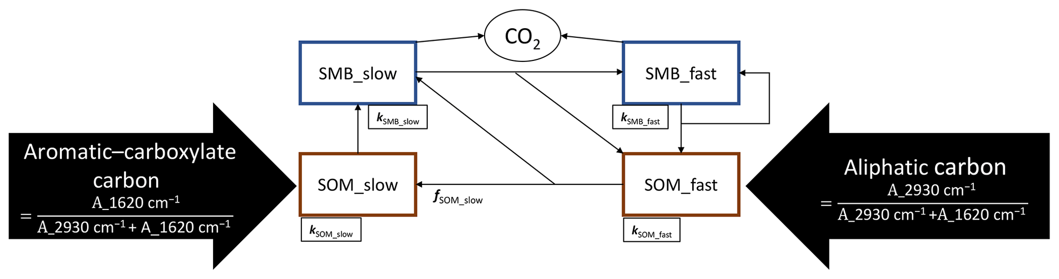
Figure 1 Original structure of the internal cycling of SOM in the Daisy model, as it was used in this study. A_2930 cm⁻¹ and A_1620 cm⁻¹ refer to the areas below the DRIFTS absorption bands at 2930 cm⁻¹ and 1620 cm⁻¹ (Eq. 3); k_SOM and k_SOM (fast and slow) are turnover rates of the fast and slow SOM and SMB pools, respectively, and f_{SOM_slow} is the humification efficiency. All model parameters can be found in Table 2.

As SOM pool sizes and turnover rates are closely linked, it could also be necessary to recalibrate Daisy parameters for the use of the DSI. Therefore, a Bayesian calibration of turnover rates was used to adjust Daisy turnover rates to the pool division and time dynamics of the measured DSI throughout the fallow period. Thus, the Daisy parameterization was evaluated with respect to equifinality and uncertainty as well as to dependence on model structure. The final hypothesis was that, through a Bayesian calibration using the DSI, Daisy pools will correspond to measured, i.e., physiochemically meaningful, fractions, thus reducing uncertainty. The posterior credibility intervals and optima of turnover rates should correspond to the results of other Bayesian calibrations carried out for similarly structured two-pool models. If such relations could be confirmed, this would point towards fundamental insights about the intrinsic SOM turnover in temperate agroecosystems.

2 Material and methods

2.1 Study sites and data used for modeling

Datasets originating from bare fallow treatments of four different sites with different experimental durations and measurement frequencies were used in this study. Topsoil (0–20 cm) samples were received from the long-term experiments of (a) the Ultuna continuous soil organic matter field experiment (established in 1956, with additional samples from 1979, 1995 and 2005 taken in autumn (Kätterer et al., 2011), four replicates) and (b) the Bad Lauchstädt extreme farmyard manure experiment (established in 1983, with additional samples from 2001, 2004 and 2008 taken in autumn (Blair et al., 2006), two replicates; https://www.ufz.de/index.php?de=37008, last access: 10 January 2019). Additional data from two medium-term bare fallow experiments (established in autumn 2009 with data until 2016) from southwest German regions were included. In these experiments three fields in the region of (c) the Kraichgau and three fields in the region of (d) the Swabian Jura, representing different climatic and geological conditions, were intensely monitored. The bare fallow plots (5 m ×5 m size) in these experiments were established within agricultural fields with three replicates per field (Ali et al., 2015). Up to four topsoil samples (0–30 cm) were taken throughout the year. Further details on all the sites can be found in Table 1. All sites had been under cultivation for at least several hundred years prior to establishing the bare fallow plots, which would suggest that a steady state could be assumed.

Table 1 Locations, soil type according to IUSS Working Group WRB 2007, initial soil organic carbon (SOC) stocks and other properties of the simulated bare fallow study sites.

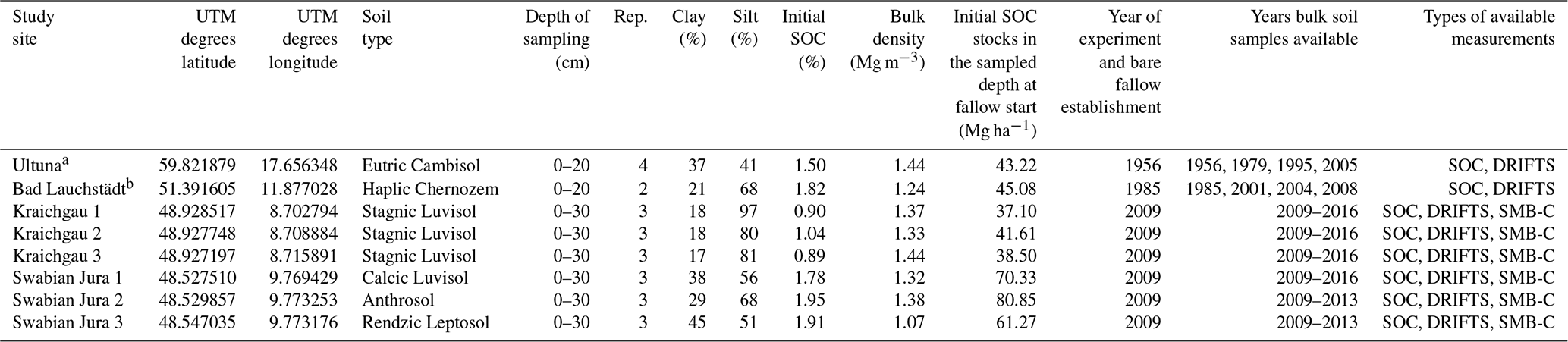
UTM, Universal Transverse Mercator reference system; SOC, soil organic carbon; Rep., replicates; SOC, soil organic carbon; DRIFTS, diffuse reflectance mid-infrared Fourier transform spectroscopy; SMB-C, soil microbial biomass carbon. ^a Ultuna continuous soil organic matter field experiment (Kätterer et al., 2011). ^b Bad Lauchstädt extreme farmyard manure experiment (Blair et al., 2006).

All available bulk soil samples of Ultuna and Bad Lauchstädt were analyzed for total organic carbon and DRIFTS spectra. For the Kraichgau and Swabian Jura sites, total organic carbon and DRIFTS spectra were measured about once every 2 years, while soil microbial biomass carbon (SMB-C) was measured up to four times per year. All bulk soil samples (except for SMB-C) were passed through a 2 mm sieve, then air-dried, ball-milled (for 2 min) to powder and stored until further analysis was carried out. Soil organic carbon (SOC) content was analyzed with a vario MAX CNS (Elementar Analysensysteme GmbH, Hanau, Germany). Soil samples for DRIFTS analysis were obtained after 24 h of drying at 32, 65 and 105 ^∘C. The dried samples were kept in a desiccator until measurement. DRIFTS spectra of bulk soil samples (with four subsamples per sample) were obtained using an HTS-XT microplate extension, mounted to a TENSOR 27 spectrometer using the processing software OPUS 7.5 (Bruker Optik GmbH, Ettlingen, Germany). A potassium bromide (KBr) beam splitter with a nitrogen-cooled HTS-XT reflection detector was used to record spectra in the mid-infrared range (4000–400 cm⁻¹). Each spectrum was a combination of 16 coadded scans with a 4 cm⁻¹ resolution. Spectra were recorded and then converted to absorbance units (AU); the acquisition mode double-sided, forward–backward and the apodization function Blackman–Harris 3 were used. After baseline correction and vector normalization of the spectra, areas below absorptions bands of interest were obtained by integration using a local baseline with the integration limits of Demyan et al. (2012). Integrated band areas of the four subsamples were then averaged. The local baselines were drawn between the intersection of the spectra and a vertical line at the integration limits (3010–2800 cm⁻¹ for the aliphatic carbon band, 1660–1580 cm⁻¹ for the aromatic–carboxylate carbon band). Example spectra and integrated band areas are displayed in Fig. S1 in the Supplement. The integration limits were selected with the goal of reducing signal interference from water and minerals, using spectra of pure substances, clay minerals and DRIFTS spectra gained during heating samples up to 700 ^∘C (Demyan et al., 2013). Particularly, the mineral interference close to the 1620 cm⁻¹ band makes accurate selection of integration limits necessary so that only its top part (assumed to consist mostly of aromatic–carboxylate carbon) is selected. In the case of our samples, the selected specific band area of the 1620 cm⁻¹ band accounted for approximately 10 % to 30 % of the band area of the larger surrounding band (Fig. S1, ca. 1755–1555 cm⁻¹). Integration limits were chosen so that the band area best corresponds to the portion that is lost with combustion or chemical oxidation (Demyan et al., 2013; Yeasmin et al., 2017). A strong correlation between the DSI and the percentage of centennially persistent SOC (r=0.84) from the combined long-term experiments used in this study (using values of centennially persistent SOC from Cécillon et al., 2018; Franko and Merbach, 2017) showed that the DSI selected in this manner did in fact explain a large portion of the SOC quality change across sites (Fig. S2).

Additionally, soils from the experiments in Kraichgau and Swabian Jura were analyzed for SMB-C using the chloroform fumigation extraction method (Joergensen and Mueller, 1996). Briefly, field-moist samples were transported to the lab in a cooler, with extractions beginning within 24 h of field sampling and the final SMB-C values corrected to an oven-dried (105 ^∘C) basis. The SMB-C was measured two to four times throughout the whole year. Stocks of SOC and SMB-C for 0–30 cm were calculated by multiplying the percentage of SOC and SMB-C with the bulk density and sampled layer thickness (Table 1), respectively. Bulk density was assumed constant for Bad Lauchstädt, Kraichgau and Swabian Jura, while for Ultuna the initial 1.44 Mg m⁻³ (Kirchmann et al., 2004) in the beginning was used for all but the last measurement, where 1.43 Mg m⁻³ (Kätterer et al., 2011) was used. Due to low coarse-fragment contents (< 5 % for Swabian Jura 3, < 2 % for Swabian Jura 1 and < 1 % for the other six sites), and because changes in stone content throughout the simulation periods are unlikely, no correction for coarse-fragment content was done.

2.2 Description of the simulation model Daisy Expert-N 5.0

All simulations were conducted using the Daisy SOM model (Hansen et al., 2012) integrated into the Expert-N 5.0 modeling framework. Expert-N 5.0 allows for a wide range of soil, plant and water models to be combined and interchanged (Heinlein et al., 2017; Klein et al., 2017; Klein, 2018). Expert-N can be compiled for both Windows and Linux systems. The Daisy model consists of two pools (fast and slow cycling) for each of the measurable fractions of (1) litter, (2) SMB and (3) stabilized SOM (Fig. 1). Due to bare fallow, litter pools were disregarded in this study, and the focus was on initializing the two SOM pools. A detailed description of the Daisy SOM submodule as it was implemented into the Expert-N 5.0 framework can be found in Mueller et al. (1997). The additional modules available for selection in the Expert-N 5.0 framework consist of a selection of established models for all simulated processes in the soil–plant continuum. The evaporation, ground heat, net radiation and emissivity were simulated according to the Penman–Monteith equation (Monteith, 1976). Water flow through the soil profile was simulated by the HYDRUS flow module (van Genuchten, 1982) with the hydraulic functions according to Mualem (1976). Heat transfer through the soil profile was simulated with the Daisy heat module (Hansen et al., 1993). In the first step of the DSI evaluation, simulations were conducted with two established parameter sets for Daisy SOM. The first set was from Mueller et al. (1997) and was a modification of the original parameter set of turnover rates reported by Jensen et al. (1997). The second set was established after calibrations made by Bruun et al. (2003) using the Askov long-term experiments, in which they introduced considerable changes to the turnover rates of the slow SOM pool and the humification efficiency. An equation developed by Bruun and Jensen (2002) was used to compute the proportions of the slow- and fast-cycling SOM pools for both parameter sets at a steady state (see next section). Parameters of both sets are given in Table 2.

Table 2 Values of the two Daisy parameter sets used in this study. The parameters consist of turnover rates (k), maintenance respiration (only for SMB, added to the turnover rate), carbon use efficiency (CUE – which divides between carbon assimilated by SMB and lost as CO₂), the humification efficiency (f_{SOM_slow}) and microbial recycling (part of SMB going directly back to SMB fast at turnover of either SMB pool). A graphical display of the model structure and pools considered within this study is found in Fig. 1.

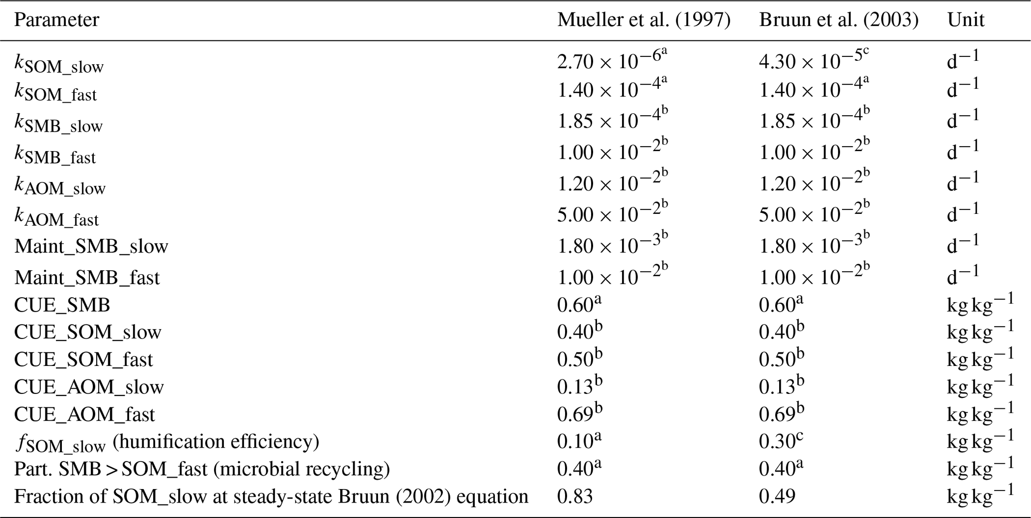
k, turnover rate (death rate for SMB); Maint, maintenance respiration (SMB only); CUE, carbon use efficiency; SOM, soil organic matter pools; SMB, soil microbial biomass pools; AOM, added organic matter pools (not considered in this study); Part., partitioning. ^a Original Jensen (1997). ^b Modified by Mueller et al. (1997). ^c Modified by Bruun et al. (2003).

For simulating soil temperature and moisture in Expert-N, daily averages of radiation, temperature, precipitation, relative humidity and wind speed are needed. For the long-term experiments they were extracted from the nearest weather station with complete data (Ultuna source specifications are as follows: Swedish Agricultural University; European Climate Assessment station ID 5506; elevation 15 m; 59.8100^∘ N, 17.6500^∘ E. Bad Lauchstädt specifications are as follows: Deutscher Wetterdienst Station 2932; elevation 131 m; 51.4348^∘ N, 12.2396^∘ E; locality name, Leipzig–Halle). For the fields of the Kraichgau and Swabian Jura, the driving variables were measured by weather stations installed next to eddy covariance stations located at the center of each field. Details on the measurements and instrumentation as well as the gap-filling methods of those eddy covariance weather stations are described in Wizemann et al. (2015).

2.3 SOM pool initializations with the DRIFTS stability index and at a steady state

Measured bulk soil SOC includes SMB-C; therefore the amount of SOC in the fast- and slow-cycling SOM pools combined consists of bulk soil SOC minus measured SMB-C. Partitioning of measured SMB-C into slow-cycling (90 %) and fast-cycling (10 %) microbial pools was carried out similarly to Mueller et al. (1998).

The remaining carbon (difference between bulk soil SOC and SMB-C) was divided between fast- and slow-cycling SOM pools either by the DRIFTS stability index (DSI) or according to the steady-state assumption. For steady-state division, the equation of Bruun and Jensen (2002) was used, which estimates the fraction of SOM in the slow pool from the model parameters under an assumed steady state:

$$\begin{array}{}\text{(1)}& \mathrm{slow}\mathrm{SOM}\mathrm{fraction}={\displaystyle \frac{\mathrm{1}}{\mathrm{1}+\frac{k_{\mathrm{SOM}\mathrm{\_}\mathrm{slow}}}{f_{\mathrm{SOM}\mathrm{\_}\mathrm{slow}}\times k_{\mathrm{SOM}\mathrm{\_}\mathrm{fast}}}}},\end{array}$$

with k_{SOM_slow} and k_{SOM_fast} representing the turnover (per day) of the slow and fast SOM pools, respectively, and f_{SOM_slow} representing the fraction of the fast SOM pool directed towards the slow SOM pool (humification efficiency). This resulted in 83 % of SOM in the slow pool for the original Daisy turnover rates and 49 % in the slow pool for the Bruun et al. (2003) turnover rates (Table 2). For the DSI initialization, the ratio of the area below the aliphatic absorption bands to the area below the aromatic–carboxylate absorption band was used as the ratio of SOM in the fast-cycling SOM pool to SOM in the slow-cycling SOM pool:

$$\begin{array}{}\text{(2)}& {\displaystyle \frac{\mathrm{fast}\mathrm{SOM}}{\mathrm{slow}\mathrm{SOM}}}={\displaystyle \frac{\mathrm{A}\mathrm{\_}\mathrm{2930}{\mathrm{cm}}^{-\mathrm{1}}}{\mathrm{A}\mathrm{\_}\mathrm{1620}{\mathrm{cm}}^{-\mathrm{1}}}}=\mathrm{DSI}.\end{array}$$

Thus, analogous to Eq. (1), the fraction of SOM in the slow pool was calculated with the formula

$$\begin{array}{}\text{(3)}& \mathrm{slow}\mathrm{SOM}\mathrm{fraction}={\displaystyle \frac{\mathrm{A}\mathrm{\_}\mathrm{1620}{\mathrm{cm}}^{-\mathrm{1}}}{\mathrm{A}\mathrm{\_}\mathrm{1620}{\mathrm{cm}}^{-\mathrm{1}}+\mathrm{A}\mathrm{\_}\mathrm{2930}{\mathrm{cm}}^{-\mathrm{1}}}},\end{array}$$

with A_2930 cm⁻¹ and A_1620 cm⁻¹ being the specific area under the aliphatic and aromatic–carboxylate band, respectively (described in Sect. 2.1). The remaining carbon was allocated to the fast SOM pool. As was mentioned before, three different data inputs for the DSI were used, obtained at drying temperatures of 32, 65 and 105 ^∘C, in order to test which drying temperature derived the best proxy for modeling. An example of the change in DRIFTS spectra occurring after several years of bare fallow can be found in Fig. 2. All DSI model initializations were simulated with both published sets of model parameters. Steady-state initializations using Eq. (1) were only simulated with the corresponding parameter set from which they were calculated.

Figure 2 Examples of baseline-corrected and vector-normalized DRIFTS spectra of bulk soil samples (dried at 105 ^∘C) of the first and last year of the bare fallow plots at four sites. Fallow periods were 50 years (a Ultuna), 24 years (b Bad Lauchstädt) and 7 years (c Kraichgau and d Swabian Jura). Small pictures in (a) to (d) are zoomed-in versions of the 2930 cm⁻¹ band (left) and the 1620 cm⁻¹ band (right). For better visibility, the full spectra pictures have a y-axis offset (+0.02 for samples from the start), while zoomed-in versions share a common baseline. More details on the sites are in Table 3.

2.4 Statistical evaluation of model performance

Statistical analysis was performed with SAS version 9.4 (SAS Institute Inc., Cary, NC, USA). To compare different model initializations, a statistical analysis of squared model errors (SME) was conducted:

$$\begin{array}{}\text{(4)}& {\mathrm{SME}}_x={\left({\mathrm{obs}}_x-{\mathrm{pred}}_x\right)}^{\mathrm{2}},\end{array}$$

with obs_x being the observed value, pred_x the predicted value and x the simulated variable of interest. A linear mixed model with SME_x as the response was then used to test for significant differences between initialization methods. This approach allowed for us to make use of the statistical power of the three Kraichgau and Swabian Jura fields to analyze which initialization was most accurate and to evaluate the trend of the model error with increasing simulation time. In some cases, SME_x were transformed to ensure a normal distribution of residuals (square root transformation for Ultuna SOC and Kraichgau and Swabian Jura SMB-C and fourth root for Kraichgau and Swabian Jura SOC), which was checked by a visual inspection of the normal Q–Q plots and histograms of residuals (Kozak and Piepho, 2018). Random effects were included to account for temporal autocorrelation of SME_x within (a) the same field and (b) the same simulation. The model reads as follows:

$$\begin{array}{}\text{(5)}& \begin{array}{rl}{y}_{ijkl}& ={\mathit{\varphi }}_{\mathrm{0}}+{\mathit{\alpha }}_{\mathrm{0}i}+{\mathit{\beta }}_{\mathrm{0}j}+{\mathit{\gamma }}_{\mathrm{0}ij}+{\mathit{\varphi }}_{\mathrm{1}}{t}_k+{\mathit{\alpha }}_{\mathrm{1}i}{t}_k\\ & +{\mathit{\beta }}_{\mathrm{1}j}{t}_k+{\mathit{\gamma }}_{\mathrm{1}ij}{t}_k+u_{kl}+u_{ijkl},\end{array}\end{array}$$

where y_ijkl are the SME_x of the simulation using the ith initialization with the jth parameter set, at the kth time in the lth field; ϕ₀ is an overall intercept; α_0i is the main effect of the ith initialization; β_0j is the main effect of the jth parameter set; γ_0ij is the ijth interaction effect of initialization ×  parameter set; ϕ₁is the slope of the time variable t_k; α_1it_k is the interaction of the ith initialization with time; β_1jt_k is the interaction of the jth parameter set with time; γ_1ijt_k is the ijth interaction effect of initialization × parameter set × time; u_kl is the autocorrelated random deviation at the kth time in the lth field; and u_ijkl is the autocorrelated residual error term corresponding to y_ijkl. The detailed SAS code can be found in the supplementary material. For Ultuna and Bad Lauchstädt, the u_kl term was left out, as both trials only had one field. As the Kraichgau and Swabian Jura sites had the exact same experimental setup and duration, these sites were jointly analyzed in the statistical model, but due to completely different setups and durations, this was not possible for Bad Lauchstädt and Ultuna. The full models with all fixed effects were used to compare different correlation structures for the random effects including (i) temporal autocorrelation (exponential, spherical, Gaussian), (ii) compound symmetry, (iii) a simple random effect for each different field and simulation, and (iv) a random intercept and slope of the time variable (with allowed covariance between both) for each field and initialization method. A residual maximum-likelihood estimation of model parameters was used, and the best-fitting random-effect structure for this model was selected using the Akaike information criterion as specified by Piepho et al. (2004). Then a stepwise model reduction was conducted until only the significant effects (p<0.05) remained in the final statistical model. Because a mixed model was used, the Kenward–Roger method was applied for estimating the degrees of freedom (Piepho et al., 2004) and to compute post hoc Tukey–Kramer pairwise comparisons of means.

2.5 Model optimization and observation weighting for Bayesian calibration

Optimization of parameters k_{SOM_slow}, k_{SOM_fast} and the humification efficiency (f_{SOM_slow}) was performed using a Bayesian calibration approach. These parameters were chosen as only they have a considerable impact on the rate of native SOM loss (see further details in the Supplement Sect. S12.2 ). The Bayesian calibration method uses an iterative process to simulate what the distribution of parameters would be given the data and the model. It combines a random walk through the parameter space with a probabilistic approach on parameter selection.

The differential evolution adaptive metropolis algorithm (Vrugt, 2016) implemented in UCODE_2014 (Lu et al., 2014; Poeter et al., 2014) was used for the Bayesian calibration in this study. As no Bayesian calibration of Daisy SOM parameters has been done before, noninformative priors were used. The main drawback of noninformative priors is that they can have longer computing times, but, as was shown by Lu et al. (2012), with sufficient data and simulation durations, the posterior distributions are very similar to using informed priors. Ranges were set far beyond published parameters with $\mathrm{1.4}\times {\mathrm{10}}^{-\mathrm{2}}$ to $\mathrm{1.4}\times {\mathrm{10}}^{-\mathrm{6}}$ d⁻¹ for k_{SOM_fast} and $\mathrm{1.4}\times {\mathrm{10}}^{-\mathrm{3}}$ to $\mathrm{5}\times {\mathrm{10}}^{-\mathrm{7}}$ d⁻¹ for k_{SOM_slow}. The parameter f_{SOM_slow} had to be more strongly constrained as without constraints it tended to run into unreasonable values of up to 99 % humification. The limits were therefore set to 0.05 to 0.35, which are ±5 % of the two published parameter sets and represent the upper boundaries of other similar models (e.g., Ahrens et al., 2014). The default UCODE_2014 Gelman–Rubin criterion (Gelman and Rubin, 1992) value of 1.2 was chosen for the convergence criteria. A total of 15 chains were run in parallel with a time step of 0.09 d in Expert-N 5.0 (this was the largest time step and fastest computation where the simulation results of water flow, temperature and hence SOM pools were unaltered compared to smaller time steps). It was ensured that at least 300 runs per chain were carried out after the convergence criterion was satisfied.

In Bayesian calibration, a proper weighing of observations is needed in order to achieve a diagonal weight matrix of residuals (proportional to the inverse of the variance–covariance matrix) and to ensure that residuals are in the same units (Poeter et al., 2005, p. 18 ff.). This included several steps. A differencing removed autocorrelation in the individual errors in each model run of the Bayesian calibration itself (the first measurement of each kind of data at each field was taken as raw data, for any repeated measurement the difference from this first measurement was taken instead of the raw data). Details on differencing are provided in chapter 3 of the UCODE_2005 manual (Poeter et al., 2005). To account for varying levels of heterogeneity of different fields in the weighting, a linear mixed model was used to separate the variance in observations from different fields originating from natural field heterogeneity from the variance originating from measurement error. To do so, a linear mixed model with a random slope and intercept of the time effect for each experimental plot was fitted to the SOC, SMB-C and DSI data for each field individually:

$$\begin{array}{}\text{(6)}& y_{kl}={\mathit{\varphi }}_{\mathrm{0}}+{\mathit{\varphi }}_{\mathrm{1}}{t}_k+u_l+u_k+u_{kl},\end{array}$$

where y_kl is the modeled variable at the kth time on the lth plot, ϕ₀ is the intercept, ϕ₁is the slope of the time variable t_k, u_l is the random intercept, u_k is the autocorrelated random deviation of the slope and u_kl is the autocorrelated residual error term corresponding to y_kl.

The error variance in each type of measurement (DSI, SMC-C, SOC) at each field ${\mathit{\sigma }}_{fM}^{\mathrm{2}}={\mathit{\sigma }}_{u_k}^{\mathrm{2}}+{\mathit{\sigma }}_{u_{kl}}^{\mathrm{2}}$ was then used for weighting of observations, excluding the field variance ${\mathit{\sigma }}_{u_l}^{\mathrm{2}}$ from the weighting scheme. This error variance was used in UCODE_2014 to compute weighted model residuals for each observation as follows:

$$\begin{array}{}\text{(7)}& \mathrm{w}\mathrm{\_}{\mathrm{SME}}_x={\displaystyle \frac{{\left({\mathrm{obs}}_x-{\mathrm{pred}}_x\right)}^{\mathrm{2}}}{{{\mathit{\sigma }}^{\mathrm{2}}}_{fM}}},\end{array}$$

where w_SME_x is the weighted squared model residual, obs_x is the observed value, pred_x is the predicted value and ${{\mathit{\sigma }}^{\mathrm{2}}}_{fM}$ is the error variance in the Mth type of measurement at each field. All w_SME_x values are summed up to the sum of squared weighted residuals, which is the objective function used in UCODE_2014 (Poeter et al., 2014). By this procedure, observations with higher measurement errors have a lower influence in the Bayesian calibration.

Since the medium-term experiments had a much higher measurement frequency, it was also tested whether giving each experiment the same weight would improve the results of the Bayesian calibration (equal weight calibration). In this case an additional group weighting term was introduced for groups of observations, representing different datasets at the different sites. This weighting term is internally multiplied with each w_SME_x value in UCODE_2014 and was calculated as

$$\begin{array}{}\text{(8)}& \mathrm{w}\mathrm{\_}{\mathrm{G}}_x={\displaystyle \frac{\mathrm{1}}{\left(n_{\mathrm{obs}}\times n_{\mathrm{par}}\times n_{\mathrm{f}}\right)}},\end{array}$$

where w_G_x is the weight multiplier for each observation, n_obs is the number of observations per parameter, n_par is the number of parameters per field, and n_f is the number of fields per site. This weighing assures that, with the exact same percentage of errors, each site would have the exact weight of 1.

The influence of several factors was assessed in this Bayesian calibration: the use of individual sites compared to combining sites, including an equal weight (EW, as described above) vs. original weight (OW) weighting only by error variance, and the effect of including and excluding the DSI (± DSI) in the Bayesian calibration. Therefore, seven Bayesian calibrations were conducted in total: (1–4) four for each individual site with original weight and the DSI, i.e., Ultuna, Bad Lauchstädt, Kraichgau and Swabian Jura; (5) equal weight calibration for all sites combined using the DSI; (6) original weight calibration for all sites combined without using the DSI in the Bayesian calibration (only for initial pool partitioning); and (7) original weight calibration for all sites combined using the DSI. The comparison of these seven Bayesian calibrations was designed to assess the effect of the site on the calibration, as well as the effect of the DSI and of user weighting decisions.

3 Results

3.1 Dynamics of SOC, SMB-C and DRIFTS during bare fallow

All bare fallow plots lost SOC over time, with the severity of SOC loss varying between soils and climates at the different sites. The Bad Lauchstädt site experienced the slowest carbon loss (7 % of initial SOC in 26 years), while SOC at Ultuna and Kraichgau was lost at much faster rates (Ultuna, 39 % of initial SOC in 50 years; Kraichgau, on average 9 % of initial SOC in 7 years; Table 3). In the Swabian Jura Field 1 the SOC loss was comparable to that of Kraichgau (about 10 % of initial SOC in 7 years) but was much less in fields 2 and 3. Some miscommunication with the field owner's contractors led to unwanted manure addition and field plowing in Swabian Jura fields 2 and 3 in 2013; hence results of these two fields after the incident in 2013 were excluded. The DRIFTS spectra revealed that the aliphatic carbon band area (2930 cm⁻¹) decreased rather fast after the establishment of bare fallow plots, while the aromatic–carboxylate band area (1620 cm⁻¹) showed only minor changes and no consistent trend (Fig. 2). The assumed fraction of SOC in the slow SOM pool according to the DSI at 105 ^∘C changed from the initial range of 54 % to 80 % to the range of 76 % to 99 % at the end of the observational period (Table 3, Fig. S3). The SMB-C reacted even more rapidly to the establishment of fallow and halved on average for all fields within a 7 year duration (Table 3).

Table 3 Measured soil properties of the bare fallow experiments at each site corresponding to the start of the bare fallow experiment and the end of the simulated period. Measurements include SOC and SMB-C stocks in the modeled layer and the percentage of SOC that would be assigned to the slow pool according to the DRIFTS stability index (DSI) measured at 105 ^∘C.

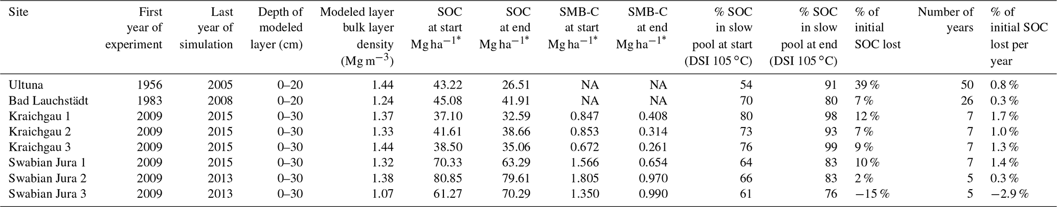
SOC, soil organic carbon; SMB-C, soil microbial biomass carbon; DSI, DRIFTS stability index; NA, no data available for this site. ^* Stocks in Mg ha⁻¹ refer to stocks within the depth of the modeled layer.

3.2 Comparison of the different model initializations

The observed trend of SOC loss with ongoing bare fallow duration was also found in all simulations (Figs. 3 and S4). For Ultuna, simulated SOC loss in all cases underestimated measured loss, while for Bad Lauchstädt, simulated SOC losses consistently overestimated measured losses. At Kraichgau sites, SOC loss was underestimated by the models but with the Bruun et al. (2003) parameter set yielding simulated values closer to actual measurements. In the Swabian Jura, both parameter sets underestimated SOC loss. The decline of SMB-C in the Kraichgau and Swabian Jura (Fig. 4) occurred more rapidly than that of SOC, though SMB-C had higher variability in measurements. The parameter sets with steady-state assumptions marked the upper and lower boundaries of the SMB-C simulations, but the DRIFTS stability index (DSI) initializations were closer to the measured values (with the exception of Swabian Jura Field 3). For brevity only simulations of Field 1 for Kraichgau and Swabian Jura are shown. Simulation results for fields 2 and 3 are found in the supplemental material (Fig. S5 for SOC simulations and Fig. S6 for SMB-C).

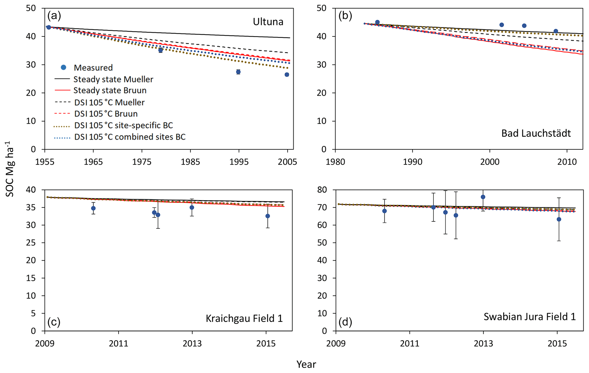
Figure 3 Example of SOC simulations from Ultuna (a), Bad Lauchstädt (b), Kraichgau Field 1 (c) and Swabian Jura Field 1 (d). Initializations were carried out (i) assuming a steady state using the formula of Bruun and Jensen (2002) (Eq. 1) with turnover rates of both Mueller et al. (1997) and Bruun et al. (2003) and (ii) by the DRIFTS stability index (DSI) at a 105 ^∘C drying temperature using both turnover rates for simulations (simulations using the other drying temperatures for the DSI are in the supplementary material). The site-specific and the combined-sites Bayesian calibrations (BC) are also displayed. Bars indicate the standard deviation of measured values of all plots (n=3) per field.

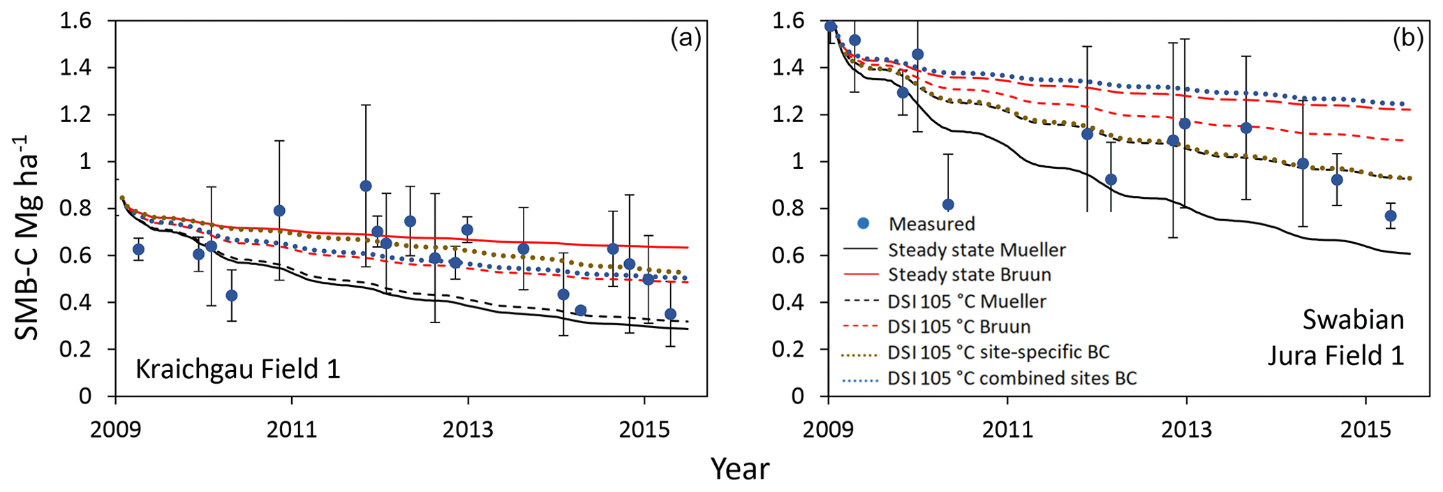
Figure 4 Example SMB-C simulations for Kraichgau Field 1 (a) and Swabian Jura Field 1 (b). Initializations were carried out (i) assuming a steady state using the formula of Bruun and Jensen (2002) with turnover rates of Mueller et al. (1997) and Bruun et al. (2003) and (ii) by the DRIFTS stability index (DSI) at a 105 ^∘C drying temperature using both turnover rates for simulations (simulations using the other drying temperatures for DRIFTS are in the supplementary material). The site-specific and the combined-sites Bayesian calibrations (BC) are also displayed. Bars indicate the standard deviation of measured values of all plots (n=3) per field.

The statistical analysis of the model error revealed the effect of the parameter set was site dependent. The three-way interaction of initialization, parameter set and time γ_1ijt_k was significant for all but Bad Lauchstädt SOC, where only the parameter set had a significant effect. In the case of Bad Lauchstädt, the model error was significantly lower with the slower Muelle (1997) SOM turnover parameter set, while for the rest of the tested cases, the faster Bruun et al. (2003) set performed significantly better (Table 4). For Ultuna and Kraichgau and Swabian Jura SOC, the steady-state assumption with Mueller et al. (1997) parameters had the highest model error, while the steady-state assumption with Bruun et al. (2003) parameters had the lowest model error of all simulations, being similar to DSI initializations at Kraichgau and Swabian Jura. However, there was a statistically significantly lower SOC model error with the DSI using the 105 ^∘C drying temperature than there was using the lower drying temperatures for the Ultuna site. For SMB-C simulations at the Kraichgau and Swabian Jura sites, however, the errors were lowest for the DSI initialization using the 105 ^∘C drying temperature with Bruun et al. (2003) parameters and significantly lower than both steady-state initializations. Of the DSI initializations using different drying temperatures, the model error was always lowest when using the 105 ^∘C drying temperature initialization compared to 32 and 65 ^∘C (significant for Ultuna, as well as for Kraichgau and Swabian Jura SMB-C using Mueller et al. (1997) parameters). As initializations with the DSI using the 105 ^∘C drying temperature consistently performed best of all three DSI initializations, only DSI spectra of soils dried at 105 ^∘C were used for the Bayesian calibration.

Table 4 Effect of the initialization method on simulation errors. Displayed are estimated least-squares means of the absolute error of Daisy bare fallow simulations of SOC and SMB-C for the sites of Ultuna, Bad Lauchstädt, and Kraichgau and Swabian Jura combined. Means are the estimate for the end of the simulation period (number of years in brackets). Different capital letters indicate significant differences (p<0.05) within columns (not tested between sites). For Bad Lauchstädt, the initialization effect was nonsignificant, so only the least-squares means for the effect of the parameter set are displayed.

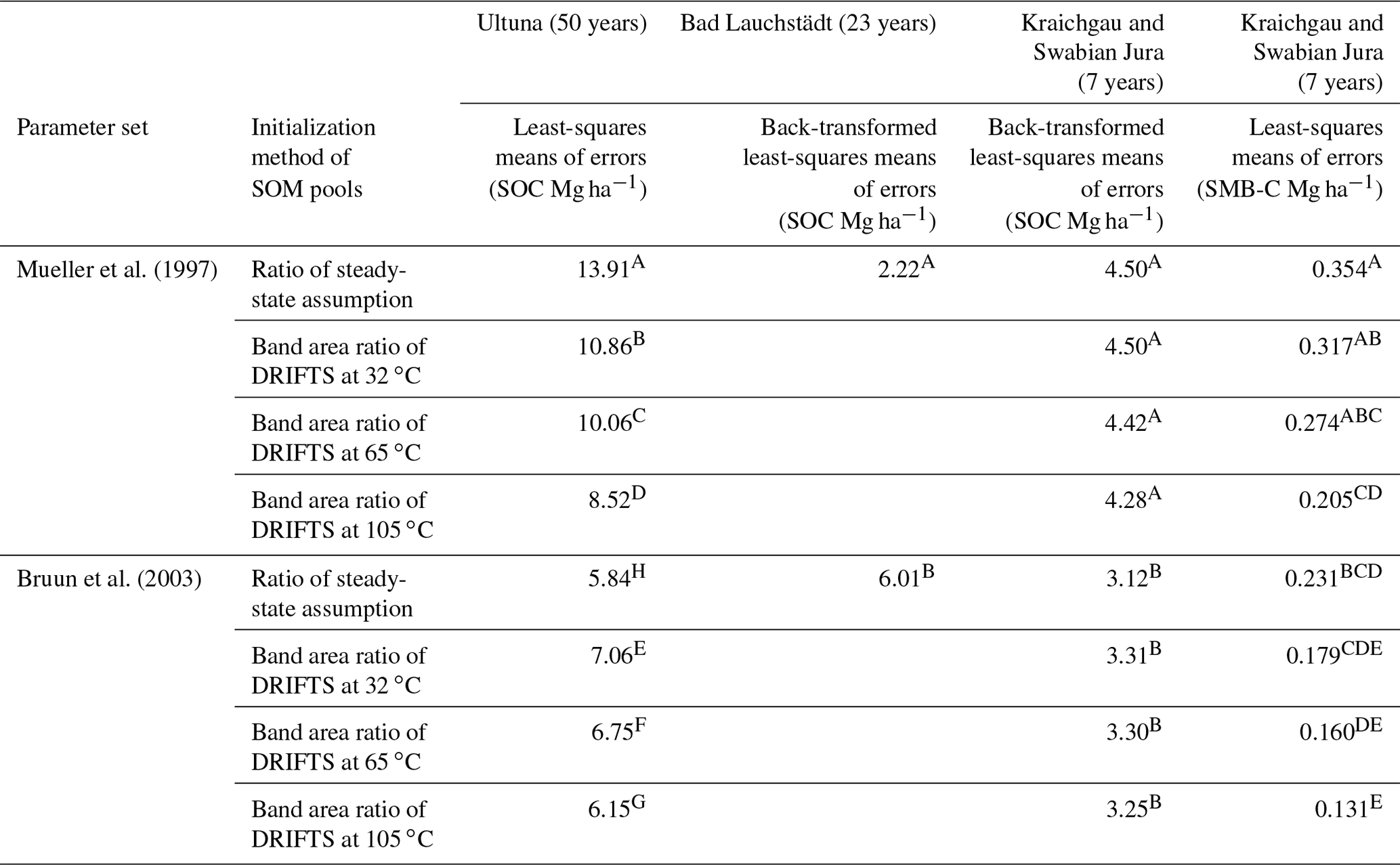
SOM, soil organic matter pools; SOC, soil organic carbon; SMB-C, soil microbial biomass carbon; DRIFTS, diffuse reflectance mid-infrared Fourier transform spectroscopy.

3.3 Informed turnover rates of the Bayesian calibration

The posterior distribution of parameters from the Bayesian calibration differed considerably between the different calibrations for individual sites, but there were also differences between different weighting schemes or when performing the Bayesian calibration without using the DSI (Fig. 5). The highest probability turnover of the fast SOM pool (k_{SOM_fast}) was 1.5 and 3 times faster for Ultuna and Kraichgau, respectively, when compared to initial rates ($\mathrm{1.4}\times {\mathrm{10}}^{-\mathrm{4}}$ d⁻¹ for both parameters sets), which fitted well for Bad Lauchstädt and Swabian Jura. For the slow SOM pools (k_{SOM_slow}), the Bad Lauchstädt, Kraichgau and Swabian Jura site calibrations were in between the two published parameter sets but tended towards the slower rates ($\mathrm{2.7}\times {\mathrm{10}}^{-\mathrm{6}}$ d⁻¹ by Mueller et al., 1997), while the optimum for Ultuna was exactly at the fast rates of Bruun et al. (2003; $\mathrm{4.3}\times {\mathrm{10}}^{-\mathrm{5}}$ d⁻¹). The humification efficiency (f_{SOM_slow}) was not strongly constrained in the Bayesian calibration, except for the Kraichgau site, where it ran into the upper boundary of 0.35. This trend towards higher humification also existed for the other sites but to a lesser extent than for Kraichgau.

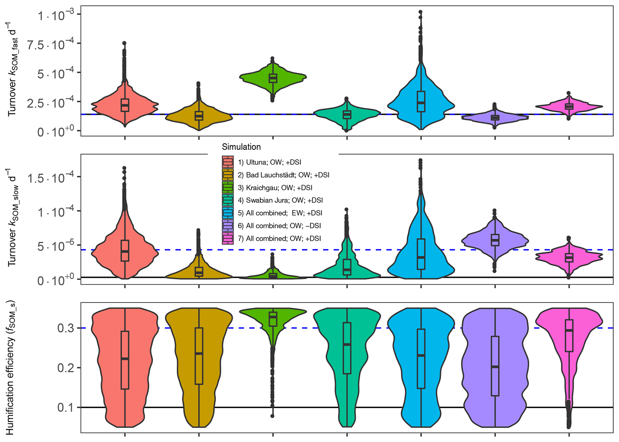
Figure 5 Violin plots of the parameter distributions, obtained by the Bayesian calibration using only the individual sites (1–4) and all sites combined (5–7) with different weighing schemes (OW, original weight; EW, equal weight calibration; ± DSI indicates whether the DSI data were used for calibration). The black line corresponds to the parameters of Mueller et al. (1997) and the dashed blue line to the parameters of Bruun et al. (2003). Note that the turnover k_{SOM_fast} parameter (top of the figure) is the same in both Mueller et al. (1997) and Bruun et al. (2003).

The different calibrations of the combination of all sites under different weightings and with or without the DSI led to considerable differences in the posteriors (Fig. 5). When combining the sites with the artificial equal weighting, the posterior distribution of all three parameters was the widest, basically covering the range of all four site calibrations. With the original weighting scheme, only informed by the variance in the data, the posteriors were narrower for all parameters, with the optima of k_{SOM_fast} being slightly faster than the two (similar) published rates. The optima of k_{SOM_slow} were slightly slower than Bruun et al. (2003) but much faster than Mueller et al. (1997), and f_{SOM_slow} was even above the higher Bruun et al. (2003) value of 0.3. The use of the original weighting scheme without the use of the DSI in the Bayesian calibration did not constrain the f_{SOM_slow} at all and had faster k_{SOM_slow} and slower k_{SOM_fast} than the one using the DSI. Both these Bayesian calibrations using the original weighting (with and without the DSI) showed a trend towards slightly faster turnover than suggested by Bruun et al. (2003).

There was a strong negative correlation between k_{SOM_fast} and k_{SOM_slow} parameters for all but the Bad Lauchstädt calibration (Fig. S7). When the DSI was not included in the Bayesian calibration, this negative correlation was stronger than when it was included (Fig. 6). The parameters k_{SOM_fast} and f_{SOM_slow} were always positively correlated, most strongly for Kraichga (0.49) and Swabian Jura (0.38) but only weakly for the long-term sites. The correlations between the parameters k_{SOM_slow} and f_{SOM_slow} were generally low and both positive and negative. The parameters with the highest probability density of the calibrations combining all sites for f_{SOM_slow}, k_{SOM_fast} and k_{SOM_slow} in that order were 0.34, $\mathrm{2.29}\times {\mathrm{10}}^{-\mathrm{4}}$ and $\mathrm{3.25}\times {\mathrm{10}}^{-\mathrm{5}}$ for the original weight calibration and 0.06, $\mathrm{9.58}\times {\mathrm{10}}^{-\mathrm{5}}$ and $\mathrm{5.54}\times {\mathrm{10}}^{-\mathrm{5}}$ for the calibration using original weights and no DSI. These results suggest that turnover rates of k_{SOM_slow} could be similar or faster than those of k_{SOM_fast} without the use of the DSI. About 10 % of the simulations of the Bayesian calibration without the DSI even had a faster k_{SOM_slow} than k_{SOM_fast}.

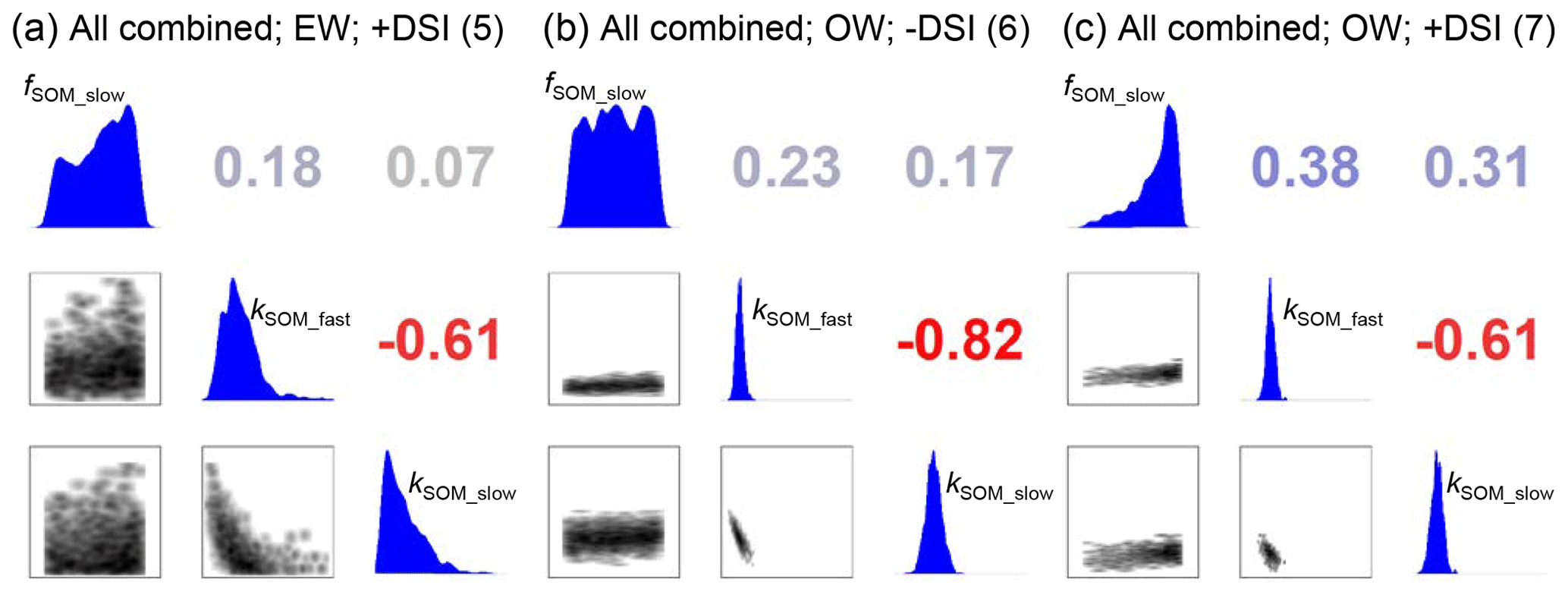
Figure 6 Correlation matrices of posterior distributions from the Bayesian calibrations of (a) equal weight calibration for all sites combined using the DSI (calibration 5), (b) original weight calibration for all sites combined without using the DSI (calibration 6) and (c) original weight calibration for all sites combined using the DSI (calibration 7). The plots of individual site simulations (calibrations 1–4) can be found in the Supplement.

4 Discussion

4.1 How useful is the DRIFTS stability index?

A search for suitable proxies for SOM pool partitioning into SOM model pools that correspond to measurable and physicochemically meaningful quantities is of high interest (Abramoff et al., 2018; Bailey et al., 2018; Segoli et al., 2013). The results of this study confirm the hypothesized usefulness of the DSI proxy in assessing the current state of SOM for pool partitioning to model SOC for several soils across Europe. This is particularly relevant given that changes in crop genotype and rotation and agricultural management and the rise of average temperatures in recent decades as well as land use changes, such as draining of soils or deforestation, in recent centuries have altered the quality and quantity of carbon inputs to soil. Consequently, the steady-state assumption for model initialization is not likely to be valid. Demyan et al. (2012) showed that, with a careful selection of integration limits for absorbance band areas, the DSI through identifying organic contributions in DRIFTS spectra is a sensitive indicator of SOM stability if mineralogy is similar (despite acknowledged mineral interference). Combined with a higher temperature (105 ^∘C) for soil drying prior to DRIFTS analysis, a strong correlation between the portion of centennially persistent SOC and the DSI (Fig. S2) was found in our study, which supports the hypothesis that the DSI might be of general applicability across sites. Results from modeling corroborated the usefulness of the DSI for SOM pool partitioning for soils of different properties across Europe. The statistical analysis of the model error for both SOC and SMB-C showed clearly that the DSI can improve poor model performance, especially when the slower turnover rates of Mueller et al. (1997) were used. When model performance is already satisfactory, the natural variability in the DSI can make model performance worse, as in the case of Ultuna SOC with Bruun et al. (2003) parameters, but this reduction was minor compared to the improvement the DSI had over steady-state assumptions at Ultuna with Mueller et al. (1997) rates. The better results for Ultuna with the Bruun et al. (2003) steady state might also just be an effect of turnover times still being too slow, and hence the more SOC in the fast pool, the faster turnover is in general and the lower the model error. This was also indicated by faster optima by the Bayesian calibration compared to both published turnover rates. In the case of the Chernozem of Bad Lauchstädt, only turnover rates had an influence on model performance and its SOC turnover was overestimated by both parameter sets (Fig. 3). It was previously suggested that the high SOC storage capacity of this site is a result of cation-bridging due to a high content of adsorbed cations (Ellerbrock and Gerke, 2018). Additionally, there is evidence of black carbon at the site (e.g., the high thermal stability found by Demyan et al., 2013). Therefore, a possible reason for an overestimation of SOC turnover in Bad Lauchstädt might be that Daisy only considers clay content as a stabilizing mechanism. Nevertheless, the use of the DSI was also suitable for Bad Lauchstädt, as there was no significant difference in model performance compared to a steady state.

The range of different sites, soils and climatic conditions of Europe represented within this study suggests the robustness of the DSI as a proxy for SOM quality and SOM pool division for a large environmental gradient. Hence, it would be an improvement over assuming a steady state of SOM wherever there is a lack of detailed information on carbon inputs and climatic conditions. Considering the timescales at which SOM develops, this is almost anywhere, as detailed data are available at best for < 200 years, which is not even one half-life of the slow SOM pool.

So far, studies that have assessed SOM quality and pool division proxies, using either the thermal stability of SOM (Cécillon et al., 2018) or size–density fractionation (Zimmermann et al., 2007), only indirectly related the proxies to inversely modeled SOM pool distributions, using machine learning and rank correlations. In contrast, our study showed that the DSI is a proxy which can be directly used for pool initialization. The DSI also makes sense from the perspective of energy content, as microorganisms can obtain more energy from the breakdown of aliphatic than aromatic–carboxylate carbon compounds (e.g., Good and Smith, 1969), and therefore aliphatic carbon is primarily targeted by microorganisms (hence has faster turnover), as previously shown for bare fallow (Barré et al., 2016).

The two distinct absorption bands for aliphatic and aromatic–carboxylate carbon bonds of the DSI fit well to the two SOM pool structures of Daisy, and the simulation of carbon flow through the soil in Daisy is very similar to several established SOM models such as SoilN, ICBM and CENTURY. It is therefore likely that, with calibration, the DSI could be used as a general proxy for SOM models with two SOM pools and a humification efficiency (f_{SOM_slow} in Daisy). The parameter correlations between k_{SOM_slow}, k_{SOM_fast} and f_{SOM_slow} according to the Bayesian calibrations also suggest that without a pool-partitioning proxy, modifying any one parameter can lead to similar results in terms of SOC and SMB-C simulation. A clear distinction between fast and slow pools needs a pool-partitioning proxy, as can be seen by faster k_{SOM_slow} than k_{SOM_fast} for some of the simulations of the Bayesian calibration without using the DSI. Assigning the DSI to Daisy reduced parameter correlations and led to a clear distinction between fast and slow SOM pools.

The DRIFTS absorption band for aliphatic carbon is most resolved when applying a 105 ^∘C drying temperature to samples prior to analysis (Laub et al., 2019). The current study's modeling results corroborated the finding that the DSI should be obtained from measurements after drying at 105  ^∘C, with the performance of the DRIFTS initializations being always in the order 105 ^∘C > 65 ^∘C > 32 ^∘C drying temperature (differences being sometimes but not always significant).

Compared with the other proxies for SOM quality discussed above, the measurements by DRIFTS are inexpensive and relatively simple, and the equipment of the same manufacturer is standardized. This should also constrain variability between different laboratories and be attractive for large-scale applications with large sample numbers, for example to initialize simulations at the regional scale. However, for standardization of the DSI for model initialization, one needs to address how the type of spectrometer (e.g., detector type) influences the spectra, if water and mineral interferences (Nguyen et al., 1991) in the spectra can be further reduced, and if a mathematical standardization of the spectra and the DSI (across instruments and water contents) is possible. While a complete elimination of mineral interference is not possible, a careful selection of integration limits and the use of a local baseline minimize mineral interference of DRIFTS spectra from bulk soils. This mostly selects the top part of the 1620 cm⁻¹ band area, which corresponds to the part that is reduced or completely lost when SOC is destroyed (Demyan et al., 2013; Yeasmin et al., 2017). Other approaches such as spectral subtraction of ashed samples or HF destruction of minerals prior to DRIFTS analysis have been developed in the attempt to obtain spectra of pure SOC. All are rather labor intensive and still produce artifacts, as it is not possible to destroy only the minerals or only the SOC without altering the respective other fraction (Yeasmin et al., 2017). Hence, we think that the selected integration limits might represent at this point the most feasible option for obtaining a robust and cost-effective proxy of SOC quality for modeling. The strong correlation of the DSI and centennially persistent SOC as well as the model results of this study seem to corroborate this. The method of DSI estimation might be improved by a study of the best integration limits optimizing the fit of the DSI and centennially persistent SOC, which would require more bare fallow experiments than in this study. From a conceptual perspective the DSI probably relates mainly to chemical recalcitrance of SOM present in different SOM fractions. In that respect it is different from physical light and heavy fraction separation approaches as each of these fractions is very heterogeneous. For example, the light fraction has strong absorbance at both aliphatic and aromatic–carboxylate carbon bands (Calderón et al., 2011), so it could be that within each fraction, aliphatic carbon is preferentially consumed by microorganisms. Thus, the DSI reflects physicochemically stabilized SOC (mainly mineral association in the case of bare soils) as also suggested by the correlation of the ratio of 1620 cm⁻¹ ∕ 2930 cm⁻¹ absorption bands to the ratio of mineral-associated carbon / light fraction carbon (Demyan et al., 2012). The relationship to mineral association in many models is represented by a texture adjustment factor. On the other hand, the DSI does not directly relate to aggregated (i.e., occluded) SOM, and its applicability in models focusing on aggregation needs to be evaluated (i.e., by a separate spectral analysis of occluded and remaining fractions).

The recent coupling of pyrolysis with DRIFTS (Nkwain et al., 2018) might be a further analytical advancement of the DSI, as it overcomes mineral interferences in the spectra. However, this technique is more complex due to a larger number of visible organic absorption bands, including CO₂ that develops from the pyrolysis, which makes it not easily applicable to established two-pool models such as Daisy. In addition, a considerable portion (30 %–40 %) of SOM is not pyrolyzed and therefore not recorded in the spectra. In summary, despite the acknowledged shortcomings, the DSI was useful to partition SOM between pools and will be even more so when the optimized parameters for the DSI are used for future applications. It seems more robust than steady-state or long-term spin-up runs which rely on strong assumptions. Further tests are needed before using the DSI for mineralogy that differs considerably from the soils of this study.

4.2 Parameter uncertainty as estimated with Bayesian calibration

According to our Bayesian calibrations, a wide range of parameter values are possible for Daisy, going far beyond the initial published parameter sets. By combining various sites and including meaningful proxies, such as the DSI, the parameter uncertainty and equifinality could be reduced and the credibility intervals narrowed. The predictions of mechanistic models usually fail to account for the three main statistical uncertainties in (1) inputs, (2) scientific judgments resulting in different model setups and (3) driving data (Wattenbach et al., 2006). However, with a Bayesian calibration framework such as that implemented in UCODE 2014, almost any model can be made probabilistic, so uncertainties in parameters and outputs can be assessed, even for projections into the future (Clifford et al., 2014). As this study focused on Bayesian calibration and we used an established model, we mainly address parameter uncertainty, although input uncertainty was also included through the weighting process. We clearly demonstrated an effect of the individual site used for Bayesian calibration on the resulting model parameters and uncertainties. Similarly diverging site-specific turnover rates were also found by Ahrens et al. (2014) in a study of soil carbon in forests. Diverging results for different sites generally point towards a need for a better understanding of the modeled system and model improvements (Poeter et al., 2005), but this often requires a deeper understanding of the system and new measurements – hence it is not always feasible. A Bayesian calibration asks the following question: what would be the probability distribution of parameters, given that the measured data should be represented by the selected model? Hence, if only one site is used, it can only answer this question for that specific site. As this study showed, the parameter set could then be highly biased for other sites. For a more robust calibration, several sites should be combined to obtain posterior distributions of parameters for a gradient of sites, though this might reduce model performance for individual sites. The introduction of the equal weighting scheme, which gave similar weights to the different sites, highlights how much bias may be introduced by user decisions of artificial weighting: this Bayesian calibration parameter set had the highest uncertainties, and it appears as if the Ultuna site had by far the strongest influence. In contrast to that, the combination of all four sites with the original weights based on the error variances or measurements led to a very clear reduction in parameter uncertainty and the narrowest parameter credibility intervals (Fig. 6a compared to Fig. 6b and c).

Table 5 Optimized turnover rates and humification efficiency of this study (using the combined site analysis with original weighting and the DSI) compared to other Bayesian calibrations and standard values of commonly used models. Turnover rates of other models were normalized to the Daisy standard of 10 ^∘C using an exponential equation (an exception was Clifford et al., 2014, where no temperature was given).

References: Ahrens et al. (2014), Bruun et al. (2003), Clifford et al. (2014), Hararuk et al. (2017), Luo et al. (2016), Mueller et al. (1997) and Parton et al. (1993). ^* Clifford et al. (2014) did not specify a base temperature for their model.

The results of the statistical analysis of model errors (Table 4) suggest that the DSI is suitable for SOC model pool initialization. This was corroborated by the Bayesian calibration, as the inclusion of the DSI narrowed credibility intervals for the slow SOM pool turnover and humification efficiency and reduced the correlation between fast and slow SOM turnover compared to the simulation without the DSI as a constraint. Especially in the case of the clear differentiation between k_{SOM_slow} and k_{SOM_fast}, our results show the advantage of attaching a physiochemical meaning to the pools that was not provided before. Other effective approaches, such as using time series of ¹⁴C data, could be combined with the DSI for better results.

Of all three parameters, the humification efficiency (f_{SOM_slow}) was the only parameter that consistently ran into the upper boundaries, set to 35 %. In fact, initial calibrations were carried out where f_{SOM_slow} was constrained to 95 %; even then, it tended to run into that constraint (Fig. S8) and led to much faster turnover rates (k_{SOM_slow}) than were published before. These values of f_{SOM_slow} were much greater than the 10 % for the Mueller et al. (1997) dataset, 30 % for Bruun et al. (2003) and other published two-pool models. Therefore, we considered the cause of the poorly constrained f_{SOM_slow} parameter to be a model formulation problem, which did not depend on whether the DSI was included in the Bayesian calibration or not. Only when the humification efficiency was restricted in the Bayesian calibration did the turnover of fast and slow SOM align with the earlier published rates. If a parameter is problematic, such as f_{SOM_slow}, it could mean that there are a lack of data. However, if parameters are constrained but run into implausible values, it usually means that the model structure is suboptimal (Poeter et al., 2005) and should be altered.

4.3 Model structure determines SOM turnover times in two-pool models

The rate of SOM decomposition remains of major interest, especially with respect to the potential of SOM as a global carbon sink (Minasny et al., 2017). Some of the first conceptual approaches proposed SOM pools with residence times of 1000 years and longer (e.g., in CENTURY, Parton et al., 1987), but the SOM models were calibrated to fit data measured in long-term experiments that included vegetation. The pool structure of early SOM models such as Daisy and CENTURY were rather similar as were the turnover rates of SOM pools (see summary in Table 5). An improved understanding of the actual number of carbon inputs to the soil, which remains challenging to measure, led to faster turnover rates in more recent model versions (e.g., by Bruun et al., 2003). The reason is probably that inputs of carbon and nitrogen to the soil were initially underestimated as it is very difficult to measure root turnover and rhizosphere exudation inputs without expensive in situ ¹³C or ¹⁴C labeling. The underestimated inputs were then likely counterbalanced in the model calibration by slower turnover rates resulting in acceptable model outputs (SOM dynamics and CO₂ emissions) for the time being. However, as our summary of more recent studies underlines (Table 5), the earlier published turnover rates seem to be subject to a systematic underestimation. As the comparison of our Bayesian calibration to other recent Bayesian calibration studies suggests, the relatively fast turnover rates of this study are in alignment with other recent findings (Table 5), as all five examples have published turnover rates for the slow SOM pool, which are at least 1 order of magnitude faster than early assumptions from the 1980s and 1990s.

It is critical to understand model uncertainties and to test fundamental assumptions of how SOM is transferred between the pools (Sulman et al., 2018). The comparison between constrained and unconstrained humification efficiency in the Bayesian calibrations suggests that the sequential flow of carbon through the system might be assuming a condensation of stabile carbon that does not actually explain the vast majority of more stable SOM formation. From a theoretical perspective, one may wonder how large amounts of less complex SOM should become complex SOM without any involvement of living soil organisms. The way that the formation of complex carbon is represented in Daisy is probably a remainder of earlier humification theories from the 1990s that mostly ignored microbe involvement, while most of the recent studies suggest that the vast majority of SOM is of microbial origin (Cotrufo et al., 2013). A simple adaption for two-pool SOM models such as Daisy that include SMB pools could acknowledge this paradigm shift: the partitioning between slow- and fast-turnover SOM could be at the death of the microbial biomass (Fig. 7) without any transfer of SOM from fast to slow pools (a brief test of this new structure is provided in Fig. S10). This would also be in alignment with the DSI concept, as aliphatic carbon should not spontaneously transform to aromatic–carboxylate carbon on its own. Then Daisy would fit better to the DSI and other proxies linking measurable fractions to SOM pools (the same is true for CENTURY and other models, which apply the same humification principle). The way that pools are linked in the current model configuration is such that the actual turnover time of recalcitrant SOM consists of the turnover of the fast and slow SOM pools combined as it moves through these pools sequentially (Fig. 1).

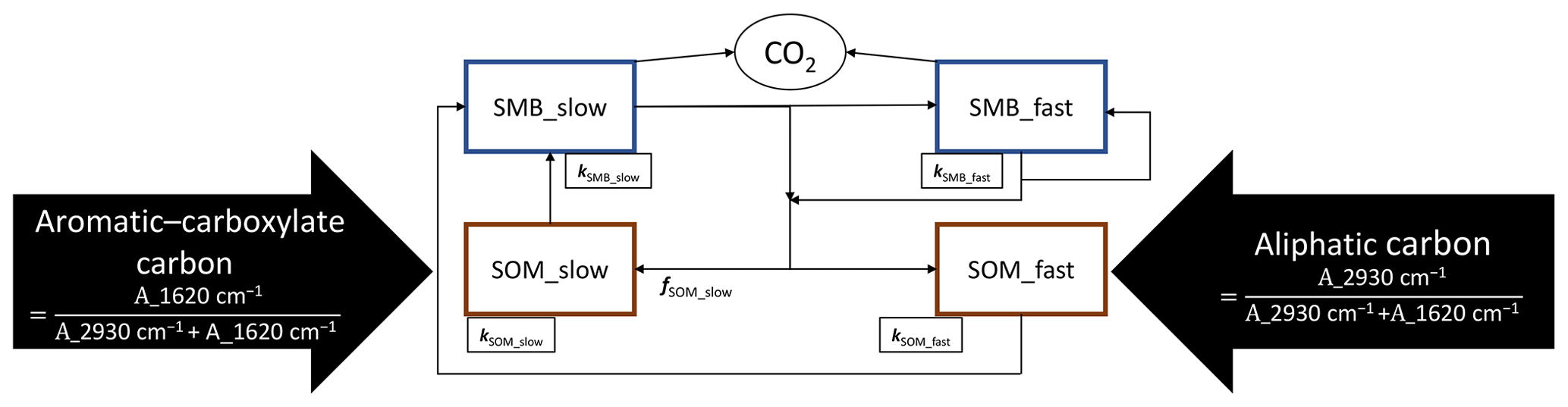
Figure 7 Suggested improvements to the internal cycling structure of SOM in the Daisy model. The division into fast- and slow-cycling SOM, corresponding to aliphatic and aromatic–carboxylate carbon follows the turnover or death of either SMB pool. Aliphatic carbon no longer becomes aromatic–carboxylate carbon without the involvement of microbes.

How strongly the basic model assumptions influence SOM simulations is also reflected when differences between one- and two-pool SOM models are compared. The turnover rates of the one-pool models are in between those of slow and fast SOM pools. However, our comparison shows that models with similar structure come to similar conclusions for SOM turnover. For example, the one-pool model in Clifford et al. (2014) was quite similar in turnover rates to that in Luo et al. (2016) but does not match well with two-pool models. Then again, the rates for the two-pool models of this study, and the studies by Ahrens et al. (2014) and Hararuk et al. (2017), were very similar in their minima and maxima, for both the slow and fast SOM pools, which shows that only models with a similar number of pools and transformations could be compared.

The 95 % credibility intervals of half-lives in Daisy were in the range from 278 to 1095 years for the slow SOM pool and from 47 to 90 years for the fast SOM pool for the combination of sites presented in this study. If these values were reasonable – and as the three recently published Bayesian calibrations including this study are quite close in turnover rates (Table 5), this seems to be the case – SOM could be lost at much faster rates under mismanagement and global warming than earlier modeling results suggest. The rates may also be biased towards an underestimation of turnover, as even with intense efforts it is next to impossible to keep bare fallow plots completely free of vegetation (weeds) and roots from neighboring plots. Recent studies are in alignment with the possibility of relatively fast SOC loss across various scales from field scale (Poyda et al., 2019) to country scale. For example in Germany, agricultural soils are much more often a carbon source than a sink (Jacobs et al., 2018). This highlights the importance of adequate SOM management and a deeper understanding of the processes at different scales. Especially in the context of understanding the response of SOM to climate change, it is not enough if the SOM balance is simulated appropriately, but fluxes within the plant–soil system also need to be quantified. The reason is that under a warmer climate and changing soil moisture levels, the plant-derived carbon inputs will change. Furthermore, soil enzymatic analysis at regional and field levels (Ali et al., 2015, 2018) suggest that pools of different complexity have different temperature sensitivities (Lefèvre et al., 2014), which is also realized in new models (Hararuk et al., 2017). If different pools have different responses to temperature, the formula by Bruun and Jensen (2002) for SOM pool distribution could not be used anymore, as it implicitly assumes a similar temperature sensitivity for all pools. In light of this, new proxies such as the DSI, soil fractionation or ¹⁴C use (Menichetti et al., 2016), which could also be combined, are crucial for making SOM pools chemically or physically meaningful and for reducing model uncertainty and equifinality. As the DSI also had a good correlation with structurally protected SOM (Demyan et al., 2012), it could also fit very well to models that directly simulate the protection of SOM as a function of microbial activity (Sulman et al., 2014). A better understanding and the use of meaningful proxies such as DRIFTS, pyrolysis with DRIFTS (Nkwain et al., 2018) or thermal deconvolution (Cécillon et al., 2018; Demyan et al., 2013) in combination with Bayesian calibration and a wide range of long-term experiments are needed. The discrepancy between simulating SOM of tropical and temperate soils, which points towards a lack of understanding of fundamental differences in processes at work on the global scale would be the best test for future proxies and SOM models, which should be facilitated by freely available datasets for model testing and calibration.

5 Conclusions

We tested the use of the DRIFTS stability index as a proxy for initializing the two SOM pools in the Daisy model and used a Bayesian calibration to implement this proxy. A statistical analysis of model errors suggested that the use of the DRIFTS stability index to initialize the fast and slow SOM pools significantly reduced model errors in most cases, especially those with initially poor performance. The DSI therefore seems to be a robust proxy for distinguishing between fast- and slow-cycling SOM in order to initialize two-pool models and adds physicochemical meaning to the pools. As other studies have also shown, statistically sound approaches such as Bayesian calibration are needed to grasp the high uncertainty in SOM turnover, which is often neglected in modeling exercises. The results of the Bayesian optimization procedure further suggest that model performance could be improved by adjusting model parameters (turnover rates, humification efficiency) in the DSI initialization approach. Meaningful proxies such as DRIFTS, physical and chemical fractionation, or ¹⁴C age assessments are likely to be the most robust way to initialize SOM pools, but their measurement method needs to be optimized to overcome known constraints, such as water and mineral interference in the case of the DSI. The results of this study suggest that the turnover of SOM could be much faster than assumed by commonly used SOM models. For example, the Daisy slow SOM pool half-life estimated in our study ranged from 278 to 1095 years (95 % credibility intervals). The variability in parameters highlights the importance of including meaningful proxies in SOM models and conducting research on a larger gradient of soils with bare fallow and planted sites and over longer time frames.