Drivers of diffusive CH₄ emissions from shallow subarctic lakes on daily to multi-year timescales

Lakes and reservoirs contribute to regional carbon budgets via significant emissions of climate forcing trace gases. Here, for improved modelling, we use 8 years of floating chamber measurements from three small, shallow subarctic lakes (2010–2017, n=1306) to separate the contribution of physical and biogeochemical processes to the turbulence-driven, diffusion-limited flux of methane (CH₄) on daily to multi-year timescales. Correlative data include surface water concentration measurements (2009–2017, n=606), total water column storage (2010–2017, n=237), and in situ meteorological observations. We used the last to compute near-surface turbulence based on similarity scaling and then applied the surface renewal model to compute gas transfer velocities. Chamber fluxes averaged 6.9±0.3 mg CH₄ m⁻² d⁻¹ and gas transfer velocities (k₆₀₀) averaged 4.0±0.1 cm h⁻¹. Chamber-derived gas transfer velocities tracked the power-law wind speed relation of the model. Coefficients for the model and dissipation rates depended on shear production of turbulence, atmospheric stability, and exposure to wind. Fluxes increased with wind speed until daily average values exceeded 6.5 m s⁻¹, at which point emissions were suppressed due to rapid water column degassing reducing the water–air concentration gradient. Arrhenius-type temperature functions of the CH₄ flux ($E_{\mathrm{a}}^{\prime }=\mathrm{0.90}\pm \mathrm{0.14}$ eV) were robust (R²≥0.93, p<0.01) and also applied to the surface CH₄ concentration ($E_{\mathrm{a}}^{\prime }=\mathrm{0.88}\pm \mathrm{0.09}$ eV). These results imply that emissions were strongly coupled to production and supply to the water column. Spectral analysis indicated that on timescales shorter than a month, emissions were driven by wind shear whereas on longer timescales variations in water temperature governed the flux. Long-term monitoring efforts are essential to identify distinct functional relations that govern flux variability on timescales of weather and climate change.

1 Introduction

Inland waters are an important source of the radiatively active trace gas methane (CH₄) to the atmosphere (Bastviken et al., 2011; Cole et al., 2007). On regional to global scales, an estimated 21 %–46 % of ice-free season CH₄ emissions from lakes, ponds, and reservoirs occur via turbulence-driven diffusion-limited gas exchange (Bastviken et al., 2011; DelSontro et al., 2018; Wik et al., 2016b) (hereafter abbreviated to “diffusive fluxes”). Diffusive fluxes are often measured with floating chambers (Bastviken et al., 2004), but gas transfer models are increasingly used, for example in regional emission budgets (Holgerson and Raymond, 2016; Weyhenmeyer et al., 2015). Fluxes computed with modelled gas transfer velocities agree to a certain extent with floating chambers and the eddy covariance technique in short-term intercomparison campaigns (Bartosiewicz et al., 2015; Crill et al., 1988; Erkkilä et al., 2018). However, long-term comparisons are needed to identify weather- and climate-related controls on the flux that are appropriate for seasonal assessments. Considering the increased use of process-based approaches in regional emission estimates (Tan and Zhuang, 2015), understanding the mechanisms that drive the components of the diffusive flux is imperative for improving emission estimates.

Drivers of diffusive CH₄ emissions

Diffusive fluxes at the air–water interface are estimated with a two-layer model (Liss and Slater, 1974):

$$\begin{array}{}\text{(1)}& F=k\left(C_{\mathrm{aq}}-C_{\mathrm{air},\mathrm{eq}}\right).\end{array}$$

The flux F (mg CH₄ m⁻² d⁻¹, hereafter abbreviated mg m⁻² d⁻¹) depends on the concentration difference across a thin layer immediately below the air–water interface (Δ[CH₄], mg m⁻³), of which the upper boundary is in equilibrium with the atmosphere (C_air,eq) and the base represents the bulk liquid (C_aq) and is limited by the gas transfer velocity k (m d⁻¹). k has been conceptualized as characterizing transfer across the diffusive boundary layer. Other models envision exchange as driven by parcels of water intermittently in contact with the atmosphere. In these surface renewal models, k depends on the frequency of the renewal events (Csanady, 2001; Lamont and Scott, 1970). The resulting calculation for k is based on the Kolmogorov velocity scale $u_{\mathit{\eta }}=(\mathit{\epsilon }\mathit{\nu }{)}^{\mathrm{1}/\mathrm{4}}$, where ε is dissipation rate of turbulent kinetic energy (TKE) and ν is kinematic viscosity (Tennekes and Lumley, 1972). Progress has been made in understanding how to compute ε and gas transfer rates as a function of wind speed and the heating and cooling at the lake's surface (Tedford et al., 2014). Comparisons between models and other flux estimation methods, such as the eddy covariance technique, illustrate the improved accuracy when computing gas transfer velocities using turbulence-based as opposed to wind-based models (Czikowsky et al., 2018; Heiskanen et al., 2014; Mammarella et al., 2015).

The supply of sparingly soluble trace gases to the air–water interface moderates fluxes when concentrations are higher within the water column than in the atmosphere. Trace gases such as CH₄ are produced in the sediments and diffuse into the overlying water. During stratification, these gases may accumulate if the density gradient restricts the efficacy of wind mixing. Thermal convection associated with surface cooling can deepen the mixed layer and transfer stored gas to the surface, enhancing emissions (Crill et al., 1988; Eugster et al., 2003). Temporal patterns of stratification and mixing contribute to variability in diffusive CH₄ fluxes (López Bellido et al., 2009; Podgrajsek et al., 2016) and concentrations (Loken et al., 2019; Natchimuthu et al., 2016). Periodic emissions from storage at depth have been particularly difficult to resolve in lake emission budgets (Bastviken et al., 2004; Wik et al., 2016b).

CH₄ emissions to the atmosphere also depend on the rates of methane metabolism regulated by substrate availability and temperature-dependent shifts in enzyme activity and microbial community structure (Borrel et al., 2011; McCalley et al., 2014; Tveit et al., 2015). Arrhenius-type relationships of CH₄ fluxes have emerged from field studies (DelSontro et al., 2018; Natchimuthu et al., 2016; Wik et al., 2014) and across latitudes and aquatic ecosystem types in synthesis reports (Rasilo et al., 2015; Yvon-Durocher et al., 2014). However, the temperature sensitivity is modulated by biogeochemical factors that differ between lake ecosystems, such as nutrient content (Davidson et al., 2018; Sepulveda-Jauregui et al., 2015), methanotrophic activity (Duc et al., 2010; Lofton et al., 2014), predominant emission pathway (DelSontro et al., 2016; Jansen et al., 2019), and warming history (Yvon-Durocher et al., 2017). In lakes, the air–water concentration difference driving the flux (Eq. 1) is further affected by factors that dissociate production from emission rates. These include biotic factors, such as aerobic and anaerobic methanotrophy, and abiotic factors such as hydrologic inputs of terrestrially produced CH₄ (Miettinen et al., 2015; Paytan et al., 2015) and storage-and-release cycles associated with transient stratification (Czikowsky et al., 2018; Jammet et al., 2017; Vachon et al., 2019). Given these interacting functional dependencies, the magnitude of fluxes has complex patterns of temporal variability.

Disentangling the physical and biogeochemical drivers of the diffusive CH₄ flux remains a challenge. The component drivers respond differently to slow and fast changes in meteorological covariates (Baldocchi et al., 2001; Koebsch et al., 2015) such that different mechanisms may explain the diel and seasonal variability of the flux. For example, temperature affects emissions through convective mixing on short timescales and through the rate of sediment methanogenesis on longer timescales; the diurnal cycle of insolation may have a limited effect on production because the heat capacity of the water buffers the temperature signal (Fang and Stefan, 1996). Similar phase lags and amplifications may lead to hysteretic flux patterns, such as cold season emission peaks due to release of gases from the hypolimnion in dimictic lakes (Encinas Fernández et al., 2014; López Bellido et al., 2009) or thermal inertia of lake sediments (Zimov et al., 1997). Spectral analysis of the flux and its components can improve our understanding of the flux variability by quantifying how much power is associated with key periodicities (Baldocchi et al., 2001).

Here we present a high-resolution, long-term dataset (2010–2017) of diffusive CH₄ fluxes from three subarctic lakes estimated with floating chambers (n=1306) and fluxes obtained by modelling using in situ meteorological observations and surface water concentrations (n=535). The surface renewal model is used to compute gas transfer velocities. Arrhenius relationships of Δ[CH₄] and fluxes of CH₄ are also calculated. Using spectral analysis of our time series data, we distinguish the temporal dependency of abiotic and biotic controls on the flux. The effects of lake size and wind exposure are illustrated by comparing results from the three different lakes.

2 Materials and methods

2.1 Field site

CH₄ emissions were measured from three subarctic lakes of postglacial origin (Kokfelt et al., 2010), located around the Stordalen Mire in northern Sweden (68^∘21^′ N, 19^∘02^′ E, Fig. 1), a palsa mire complex underlain by discontinuous permafrost (Malmer et al., 2005). The Mire (350 m a.s.l.) is part of a catchment that connects Mt. Vuoskoåiveh (920 m a.s.l.) in the south to Lake Torneträsk (341 m a.s.l.) in the north (Lundin et al., 2016; Olefeldt and Roulet, 2012). Villasjön is the largest and shallowest of the lakes (0.17 km², 1.3 m max. depth) and drains through fens into a stream feeding Mellersta Harrsjön and Inre Harrsjön, which are 0.011 and 0.022 km² in size and have maximum depths of 6.7 m and 5.2 m, respectively (Wik et al., 2011). The lakes are normally ice-free from the beginning of May through the end of October. Manual observations were generally conducted between mid-June and the end of September. Diffusion accounts for 17 %, 52 %, and 34 % of the ice-free CH₄ flux in Villasjön, Inre, and Mellersta Harrsjön, respectively, with the remainder emitted via ebullition (2010–2017; Jansen et al., 2019).

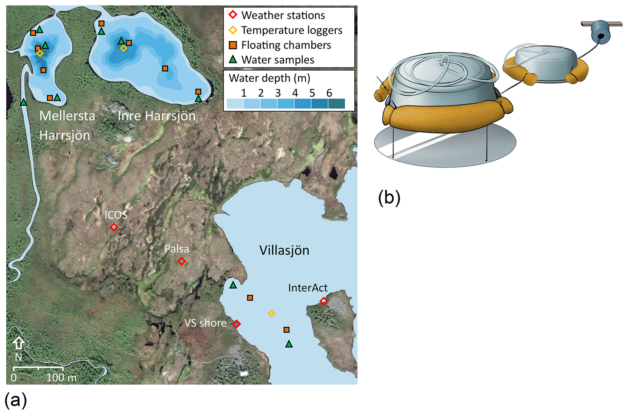
Figure 1 Map of the Stordalen Mire field site (a). Chamber and sampling locations are shown as they were in 2015–2017. A schematic of the floating chamber pairs is shown in (b). Lake bathymetry from Wik et al. (2011). Satellite imagery: ©Google, DigitalGlobe, 2017.

2.2 Floating chambers

We used floating chambers to directly measure the turbulence-driven diffusive CH₄ flux across the air–water interface (Fig. 1). They consisted of plastic tubs covered with aluminium tape to reflect incoming radiation and were equipped with polyurethane floats and flexible sampling tubes capped at one end with three-way stopcocks (Bastviken et al., 2004). Depending on flotation depth, each chamber covered an area between 610 and 660 cm² and contained a headspace of 4 to 5 L. Chambers were deployed in pairs with a plastic shield mounted 30 cm below one chamber of each pair to deflect methane bubbles rising from the sediment. Every 1–2 weeks during the ice-free seasons of 2010 to 2017, two to four chamber pairs were deployed in Villasjön and four to seven chamber pairs were deployed in Inre and Mellersta Harrsjön in different depth zones (Fig. 1). The number of chambers and deployment intervals exceeded the minimum needed to resolve the spatio-temporal variability of the flux (Wik et al., 2016a). Over a 24 h period, two to four 60 mL headspace samples were collected from each chamber using polypropylene syringes, and the flotation depth and air temperature were noted in order to calculate the headspace volume. The 24 h deployment period integrates diel variations in the gas transfer velocity (Bastviken et al., 2004).

The fluxes reported here are from the shielded chambers only. To check that the shields were not reducing fluxes from turbulent processes such as convection, we compared fluxes from shielded and unshielded chambers on days when the lake mean bubble flux was < 1 % of the lake mean diffusive flux (bubble traps, 2009–2017; Jansen et al., 2019; Wik et al., 2013). Averaged over the three lakes, the difference was statistically significant (0.20±0.16 mg m⁻² d⁻¹, n=58, mean ±95 % CI), but small in relative terms (6 % of the mean flux). Conversely, some types of floating chambers can enhance gas transfer by creating artificial turbulence when dragging through the water (Matthews et al., 2003; Vachon et al., 2010; Wang et al., 2015). Ribas-Ribas et al. (2018), Banko-Kubis et al. (2019), and Gålfalk et al. (2013) assessed gas transfer velocities in floating chambers of similar design, size, and flotation depth as those used in this study. Ribas-Ribas et al. (2018) and Banko-Kubis et al. (2019) measured TKE dissipation rates with acoustic Doppler velocimetry (ADV) inside and outside the chamber perimeter and concluded that the chambers did not cause artificial turbulence. Gålfalk et al. (2013) similarly found good agreement between k₆₀₀ derived from free-floating chamber observations with a CH₄ tracer and k₆₀₀ computed independently from nearby ADV measurements and an infrared (IR) imaging technique.

2.3 Water samples

Surface water samples were collected 0.2–0.4 m below the surface at two to three different locations in each lake, at 1- to 2-week intervals from June to October (Fig. 1). Samples were collected from the shore with a 4 m Tygon tube attached to a float to avoid disturbing the sediments (2009–2014) and from a rowboat over the deepest points of Inre and Mellersta Harrsjön (2010–2017) and at shallows (< 1 m water depth) on either end of the lakes (2015–2017) using a 1.2 mL × 3.2 mm i.d. Tygon tube. In addition, water samples were collected at the deepest point of Inre and Mellersta Harrsjön at 1 m intervals down to 0.1 m from the sediment surface with a 7.5 mL × 6.4 mm i.d. fluorinated ethylene propylene (FEP) tube. Subsequently, 60 mL polypropylene syringes were rinsed thrice with sample water before duplicate bubble-free samples were collected and were capped with airtight three-way stopcocks. The 30 mL samples were equilibrated with 30 mL headspace and shaken vigorously by hand for 2 min (2009–2014) or on a mechanical shaker at 300 rpm for 10 min (2015–2017). Prior to 2015, outside air – with a measured CH₄ content – was used as headspace. From 2015 on we used an N₂ 5.0 headspace (Air Liquide). Water sample conductivity was measured over the ice-free season of 2017 (n=323) (S230, Mettler-Toledo) and converted to specific conductance using a temperature-based approach.

2.4 Concentration measurements

Gas samples were analysed within 24 h after collection at the Abisko Scientific Research Station, 10 km from the Stordalen Mire. Sample CH₄ contents were measured on a Shimadzu GC-2014 gas chromatograph which was equipped with a flame ionization detector (GC–FID) and a 2.0 m long, 3 mm i.d. stainless-steel column packed with 80∕100 mesh HayeSep Q and used N₂ > 5.0 as a carrier gas (Air Liquide). For calibration we used standards of 2.059 ppm CH₄ in N₂ (Air Liquide). A total of 10 standard measurements were made before and after each run. After removing the highest and lowest values, relative standard deviations of the standard runs were generally less than 0.25 %.

2.5 Water temperature, pressure, density, and mixed-layer depth

Water temperature was measured every 15 min from 2009 to 2018 with temperature loggers (HOBO Water Temp Pro v2, Onset Computer) in Villasjön and at the deepest locations within Inre and Mellersta Harrsjön. Sensors were deployed at 0.1, 0.3, 0.5, and 1.0 m depth in all lakes, with additional sensors at 3.0, 5.0 m (IH and MH), and 6.7 m (MH). Sensors were intercalibrated prior to deployment in a well-mixed water tank and by comparing readouts just before and during the onset of freezing when the water column was isothermal. In this way a precision of < 0.05 ^∘C was achieved. The bottom sensors were buried in the surface sediment and were excluded from in situ intercalibration. Water pressure was measured in Mellersta Harrsjön (5.5 m) with a HOBO U20 water level logger (Onset Computer). Water density was computed from temperature and salinity (Chen and Millero, 1977), using lake-averaged specific conductivity and a salinity factor (mS cm⁻¹) × (g kg⁻¹)⁻¹ of 0.57. The salinity factor was based on a linear regression of simultaneous measurements of conductivity and dissolved solids (R²=0.99, n=7) in five lakes in the Torneträsk catchment (Miljödata-MVM, 2017). We defined the depth of the surface mixing layer (z_mix) at a density gradient threshold (dρ ∕ dz) of 0.03 kg m⁻³ m⁻¹ (Rueda et al., 2007).

2.6 Meteorology

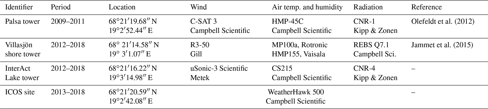
Meteorological data were collected from four different masts on the Mire and collectively covered a period from June 2009 to October 2018 with half-hourly measurements of wind speed, air temperature, relative humidity, air pressure, and irradiance (Fig. 1, Table 1). Wind speed was measured with 3D sonic anemometers at the Palsa tower (z=2.0 m), the Villasjön shore tower (z=2.9 m), the InterAct Lake tower (z=2.0 m), and the Integrated Carbon Observation System (ICOS) site (z=4.0 m). Air temperature and relative humidity were measured at the Palsa tower, at the Villasjön shore tower (Rotronic MP100a (2012–2015)/Vaisala HMP155 (2015–2017)), and at the InterAct lake tower. Incoming and outgoing shortwave and long-wave radiation were monitored with net radiometers at the Palsa tower (Kipp & Zonen CNR1) and at the InterAct lake tower (Kipp & Zonen CNR4). Precipitation data were collected with a WeatherHawk 500 at the ICOS site. Overlapping measurements were cross-validated and averaged to form a single time series.

Table 1 Location and instrumentation of meteorological observations on the Stordalen Mire, 2009–2018.

2.7 Computation of CH₄ storage and residence time

The amount of CH₄ stored in the water column (g CH₄ m⁻²) was computed by weighting and then adding each concentration measurement by the volume of the 1 m depth interval within which it was collected. For the upper 2 m of the two deeper lakes, we separately computed storage in the vegetated littoral zone from nearshore concentration measurements, as these values could be different from those further from shore due to outgassing and oxidation during horizontal transport (DelSontro et al., 2017). We computed the average residence time of CH₄ in the lake by dividing the amount stored by the lake mean surface flux. Residence times computed with this approach should be considered upper limits, because in this calculation we assumed that removal processes other than surface emissions, such as microbial oxidation, were negligible or took place at the sediment–water interface with minimal effect on water column CH₄.

2.8 Flux calculations

In order to calculate the chamber flux with Eq. (1), we estimated the gas transfer velocity, k_ch (cm h⁻¹), from the time-dependent equilibrium chamber headspace concentration C_h,eq(t) (mg m⁻³) (Bastviken et al., 2004):

$$\begin{array}{}\text{(2)}& \left(C_{\mathrm{aq}}-C_{\mathrm{h},\mathrm{eq}}\left(t\right)\right)=\left(C_{\mathrm{aq}}-C_{\mathrm{h},\mathrm{eq}}\left(t_{\mathrm{0}}\right)\right)e^{-\frac{K_{\mathrm{H}}R{T}_{\mathrm{water}}A}{V}{k}_{\mathrm{ch}}t},\end{array}$$

where K_H is Henry's law constant for CH₄ (mg m⁻³ Pa⁻¹) (Wiesenburg and Guinasso, 1979), R is the universal gas constant (m³ Pa mg⁻¹ K⁻¹), T_water is the surface water temperature (K), and V and A are the chamber volume (m³) and area (m²), respectively. This method accounts for gas accumulation in the chamber headspace, which reduces the concentration gradient and limits the flux (Eq. 1) (Fig. 2). For a subset of chamber measurements where simultaneous water concentration measurements were unavailable (n=949) we computed the flux from the headspace concentrations alone:

$$\begin{array}{}\text{(3)}& F=c_{\mathrm{1}}M{\displaystyle \frac{\partial x_{\mathrm{h}}}{\partial t}}{\displaystyle \frac{\mathrm{PV}}{R{T}_{\mathrm{air}}A}}.\end{array}$$

$\partial x_h/\partial t$ is the headspace CH₄ mole fraction change (mol mol⁻¹ d⁻¹) computed with ordinary least-squares (OLS) linear regression (Fig. 2), M is the molar mass of CH₄ (0.016 mg mol⁻¹), P is the air pressure (Pa), and T_air is the air temperature (K). Scalar c₁ corrects for the accumulation of CH₄ gas in the chamber headspace and increases over the deployment time. Comparing both chamber flux calculation methods, we find c₁=1.21 for 24 h deployments (OLS, R²=0.85, n=357). Chambers were sampled up to four times during their 24 h deployment (at 10 min, 1–5 h, and 24 h), which allowed us to compute fluxes at time intervals of 1 and 24 h. P and T_air were averaged over the relevant time interval.

Figure 2 shows that the headspace correction is necessary to avoid underestimating fluxes. The headspace-corrected flux (dashed red line) equals the initial slope of Eq. (2) (solid red line) and is about 21 % higher than the non-corrected flux (lower dashed black line in Fig. 2). However, both Eq. (2) (solid red line) and Eq. (3) with c₁=1 (dashed black lines) fit the concentration data (R²≥0.98 for 94 % of 24 h flux measurements). This similarity results partly because the fluxes were low enough to keep headspace concentrations well below equilibrium with the water column. Short-term measurements (upper dashed black line) may omit the need for headspace correction (Bastviken et al., 2004). Because concentration measurements were not available for all chamber observations, we used multi-year mean values of Δ[CH₄] and k_ch to compute c₁ as a function of chamber deployment time. For 24 h chamber deployments, c₁=1.21.

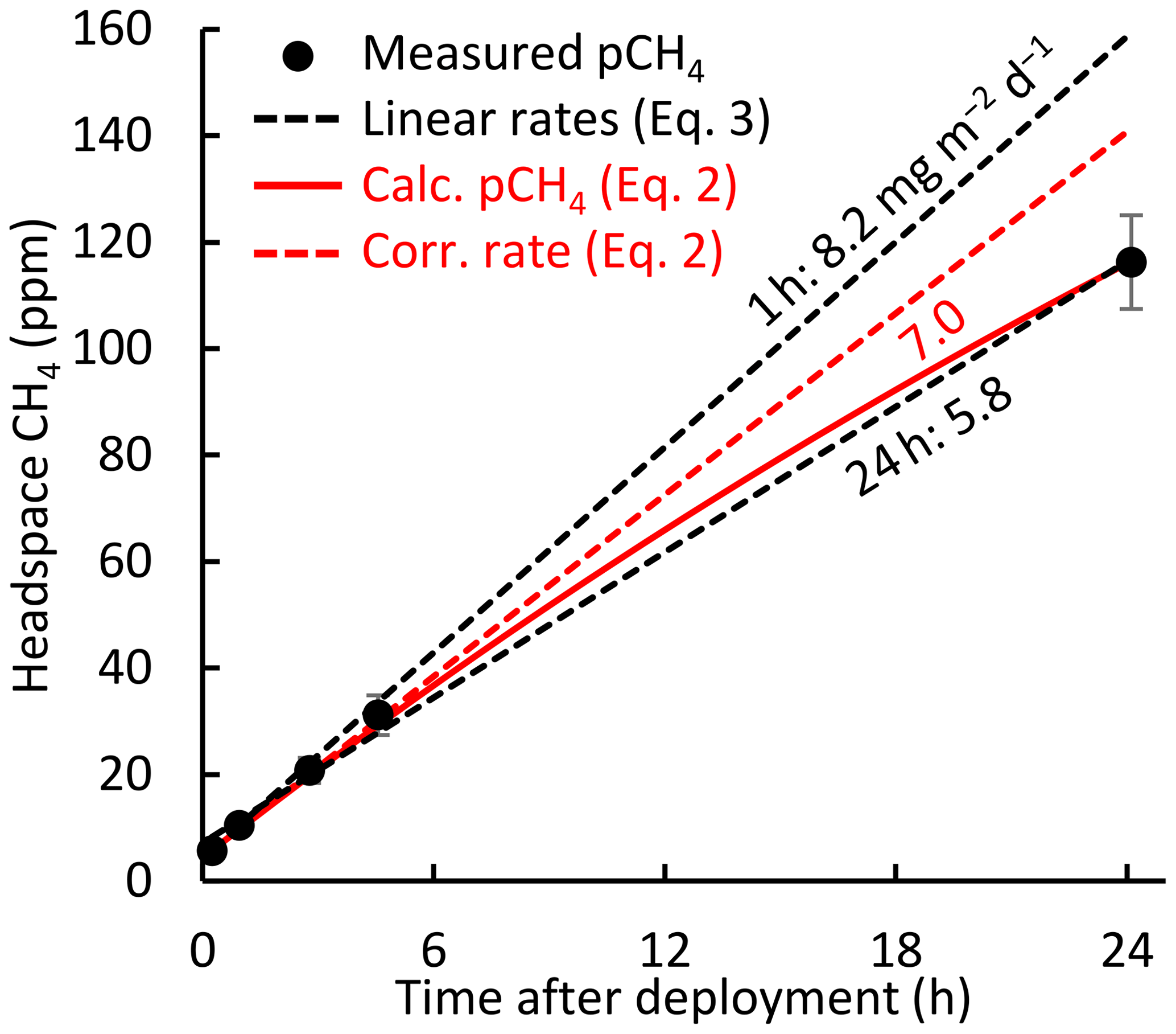
Figure 2 Example of chamber headspace CH₄ concentrations versus deployment time. Measured concentrations (dots) are averages from 2015 to 2017 (0.1 h) and 2011 (1–24 h); error bars represent the 95 % confidence intervals. Linear regressions (dashed black lines) show the rate increase over 1 h (two measurements) and over 24 h (five measurements). The solid red line represents chamber concentrations computed with Eq. (2). The rate increase associated with the mean 24 h flux corrected for headspace accumulation is shown as a dashed red line (Eq. 1 with k_ch from Eq. 2, or Eq. 3 with c₁=1.21). Labels denote fluxes calculated from the linear regression slopes (Eq. 3, black) and from Eq. (2) (red).

2.9 Computing gas transfer velocities with the surface renewal model

We used the surface renewal model (Lamont and Scott, 1970) formulated for small eddies at Reynolds numbers > 500 (MacIntyre et al., 1995; Theofanous et al., 1976) to estimate k:

$$\begin{array}{}\text{(4)}& k_{\mathrm{mod}}=\mathit{\alpha }{\left(\mathit{\epsilon }\mathit{\nu }\right)}^{\frac{\mathrm{1}}{\mathrm{4}}}{\mathit{\text{Sc}}}^{-\frac{\mathrm{1}}{\mathrm{2}}},\end{array}$$

where the hydrodynamic and thermodynamic forces driving gas transfer are expressed, respectively, as the TKE dissipation rate ε (m² s⁻³) and the dimensionless Schmidt number Sc, defined as the ratio of the kinematic viscosity v (m² s⁻¹) to the free solution diffusion coefficient D₀ (m² s⁻¹) (Jähne et al., 1987; Wanninkhof, 2014). The scaling parameter α has a theoretical value of 0.37 (Katul et al., 2018) but is often estimated empirically (α^′) to calibrate the model (e.g. Wang et al., 2015). To allow for a qualitative comparison between model and chamber fluxes, we took ratios of k_ch (floating chambers) and (εν)^¼ Sc^−½ (surface renewal model, half-hourly values of k_mod averaged over each chamber deployment period) and determined ${\mathit{\alpha }}^{\prime }=\mathrm{0.23}\pm \mathrm{0.02}$ for all lakes (mean ±95 % CI, n=334) (Fig. 3), ${\mathit{\alpha }}^{\prime }=\mathrm{0.31}\pm \mathrm{0.06}$ (n=67) for Villasjön, ${\mathit{\alpha }}^{\prime }=\mathrm{0.25}\pm \mathrm{0.03}$ (n=136) for Inre Harrsjön, and ${\mathit{\alpha }}^{\prime }=\mathrm{0.17}\pm \mathrm{0.0}$2 (n=131) for Mellersta Harrsjön (Supplement Fig. S1). Calibrating the model in this way allowed us to assess whether chamber flux relationships with wind speed and temperature were reproduced by the model. For similar comparative purposes, k values were normalized to a Schmidt number of 600 (CO₂ at 20 ^∘C) (Wanninkhof, 1992): $k_{\mathrm{600}}={\left(\mathrm{600}/\mathit{\text{Sc}}\right)}^{-\mathrm{0.5}}k$. The wind speed at 10 m (U₁₀) was computed from measured wind speed following Smith (1988), assuming a neutral atmosphere.

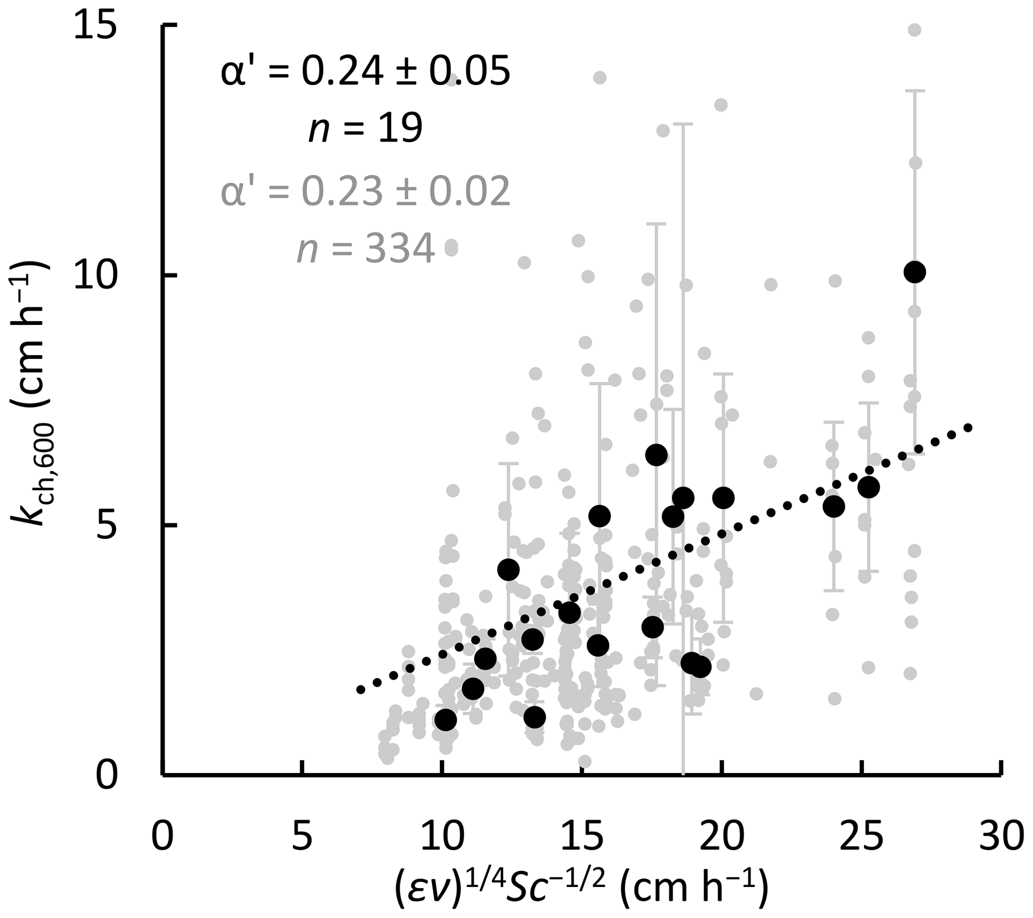
Figure 3 Determination of the model scaling parameter α^′ via comparison between gas transfer velocities from floating chambers (Eq. 2) and the surface renewal model (Eq. 4 with ${\mathit{\alpha }}^{\prime }=\mathrm{1}$ and Sc = 600, half-hourly values averaged over each chamber's 24 h deployment period) for all three lakes. Dots represent individual chamber deployments (grey) and multi-chamber means for each weekly deployment in 2016 and 2017, when concentration measurements were taken simultaneously with, and in close proximity to, the chamber measurements (black). Mean ratios, and therefore α^′, are represented by the slopes of the dotted lines. Error bars represent 95 % confidence intervals of the means.

We used a parametrization by Tedford et al. (2014) based on Monin–Obukhov similarity theory to estimate the TKE dissipation rate at half-hourly time intervals:

$$\begin{array}{}\text{(5)}& \mathit{\epsilon }=\left\{\begin{array}{ll}\mathrm{0.56}{u}_{\ast w}^{\mathrm{3}}/\mathit{\kappa }z+\mathrm{0.77}\mathit{\beta }& \mathrm{if}\mathit{\beta }>\mathrm{0}\left(\mathrm{cooling}\right)\\ \mathrm{0.6}{u}_{\ast w}^{\mathrm{3}}/\mathit{\kappa }z& \mathrm{if}\mathit{\beta }\le \mathrm{0}\left(\mathrm{heating}\right),\end{array}\right.\end{array}$$

where u_∗w is the water friction velocity (m s⁻¹), κ is the von Kármán constant, and z is depth below the water surface (0.15 m, the depth for which Eq. 5 was calibrated). We determined u_∗w from the air friction velocity u_∗a assuming equal shear stresses (τ) on both sides of the air–water interface, $\mathit{\tau }={\mathit{\rho }}_{\mathrm{a}}{u}_{\ast a}^{\mathrm{2}}={\mathit{\rho }}_{\mathrm{w}}{u}_{\ast w}^{\mathrm{2}}$, and taking into account atmospheric stability (MacIntyre et al., 2014; Tedford et al., 2014). β is the buoyancy flux (m² s⁻³), which accounts for turbulence generated by convection (Imberger, 1985):

$$\begin{array}{}\text{(6)}& \mathit{\beta }={\mathit{\alpha }}_{\mathrm{T}}g{Q}_{\mathrm{eff}}/c_{\mathrm{pw}}{\mathit{\rho }}_{\mathrm{w}}.\end{array}$$

Here, α_T is the thermal expansion coefficient (m³ K⁻¹) (Kell, 1975), g is the standard gravity (m s⁻²), c_pw (J kg⁻¹ K⁻¹) is the water specific heat, and ρ_w (kg m⁻³) is the water density. Q_eff (W m⁻²) represents the net heat flux into the mixing layer and is the sum of net shortwave and long-wave radiation and sensible and latent heat fluxes. Penetration of radiation into the water column was evaluated across seven wavelength bands via Beer's law (Jellison and Melack, 1993). An attenuation coefficient of 0.74 was computed for the visible portion of the spectrum from Secchi depth (2.3 m; Karlsson et al., 2010) following Idso and Gilbert (1974). Net long-wave radiation (LW_net= LW_out− LW_in) was computed via measurements of LW_in (Table 1) and LW_out=σT⁴, where σ is the Stefan–Boltzmann constant ($\mathrm{5.67}\times {\mathrm{10}}^{-\mathrm{8}}$ W m⁻² K⁻⁴) and T is the surface water temperature in kelvin. LW_net time series were gap-filled with ice-free mean values for each lake. Sensible and latent heat fluxes were computed with the bulk aerodynamic formula (MacIntyre et al., 2002). Both Q_eff and β are here defined as positive when the heat flux is directed out of the water, for example when the surface water cools.

Direct measurements of ε in an Arctic pond (1 m depth, 0.005 km² surface area) demonstrate that Eq. (5) can characterize near-surface turbulence in small, sheltered water bodies similar to the lakes studied here (MacIntyre et al., 2018). When the near surface was strongly stratified at instrument depth (buoyancy frequencies ($N=\sqrt{g/{\mathit{\rho }}_{\mathrm{w}}\times \mathrm{d}{\mathit{\rho }}_{\mathrm{w}}/\mathrm{d}z}$) > 25 cycles per hour, cph), the required assumption of homogeneous isotropic turbulence was not met and Eq. (5) could not be evaluated. We observed cases with N>25 cph < 3 % of the time.

2.10 Calculation of binned means

We binned data to assess correlations between the flux and environmental covariates. Half-hourly values of water temperature and wind speed were averaged over the deployment period of each chamber (fluxes) and over 24 h prior to the collection of each water sample (concentrations), reflecting the mean residence time of CH₄ in the water column. Fluxes, concentrations, and k values were then binned in 10 d, 1 ^∘C, and 0.5 m s⁻¹ bins to obtain relationships with time, water temperature, and wind speed, respectively. The 10 d bins typically contained at least 1 sampling day for each overlapping year and enabled representative averaging across years. Lake-dependent variables (e.g. flux) were normalized by lake to obtain a single time series (divided by the lake mean, multiplied by the overall mean).

2.11 Calculation of the empirical activation energy

Chamber and modelled fluxes as well as concentrations were fitted to an Arrhenius-type temperature function (e.g. Wik et al., 2014; Yvon-Durocher et al., 2014):

$$\begin{array}{}\text{(7)}& F=e^{-E_{\mathrm{a}}{}^{\prime }/k_{\mathrm{B}}T+b},\end{array}$$

where k_B is the Boltzmann constant ($\mathrm{8.62}\times {\mathrm{10}}^{-\mathrm{5}}$ eV K⁻¹) and T is the water temperature in kelvin. The empirical activation energy (E_a^′, in electron volts (eV), 1 eV = 96 kJ mol⁻¹) was computed with a linear regression of the natural logarithm of the fluxes and concentrations onto the inverse temperature (K⁻¹), of which b is the intercept.

2.12 Timescale analysis: power spectra and climacogram

We computed power spectra for near-continuous time series of the surface sediment, water and air temperature, and wind speed according to Welch's method (pwelch in MATLAB 2018a), which splits the signal into overlapping sections and applies a cosine tapering window to each section (Hamming, 1989). Data gaps were filled by linear interpolation. We removed the linear trend from the original time series to reduce red noise, and we block-averaged spectra (eight segments with 50 % overlap) to suppress aliasing at higher frequencies. We normalized the spectral densities by multiplying by the frequency and dividing by the variance of the original time series (Baldocchi et al., 2001).

We evaluated our discontinuous (fluxes, concentrations) and continuous (meteorology) time series with a climacogram, an intuitive way to visualize a continuum of variability (Dimitriadis and Koutsoyiannis, 2015). It displays the change of the standard deviation (σ) with averaging timescale (t_avg). Variables were normalized by lake to create a single time series at half-hourly resolution (e.g. 48 entries for each 24 h chamber flux). To compute each standard deviation (σ(t_avg)) data were binned according to averaging timescale, which ranged from 30 min to 1 year. Because of the discontinuous nature of the datasets, n bins were distributed randomly across the time series. We chose n=100 000 to ensure that the 95 % confidence interval of the standard deviation at the smallest bin size was less than 1 % of the value of σ (Sheskin, 2007). To allow for comparison between variables, we normalized each σ series by its initial smallest-bin value: ${\mathit{\sigma }}_{\mathrm{norm}}=\mathit{\sigma }/{\mathit{\sigma }}_{\mathrm{init}}$. For timescales < 1 week we used 1 h chamber observations, noting that sparse daytime-only observations of concentrations and 1 h fluxes may underestimate short-term variability (σ_init). We use the climacogram to test whether the variability of the diffusive CH₄ flux is contained within meteorological variability, as for terrestrial ecosystem processes (Pappas et al., 2017).

2.13 Statistics

We used analysis of variance (ANOVA) and the t test to compare means of different groups. The use of means, rather than medians, was necessary because annual emissions can be determined by rare high-magnitude emission events. Parametric tests were justified because of the large number of samples in each analysis, in accordance with the central limit theorem. Linear regressions were performed with the ordinary least-squares method (OLS): reported p values refer to the significance of the regression slope. Non-linear regressions were optimized with the Levenberg–Marquardt algorithm for non-linear least squares with confidence intervals based on bootstrap replicates (n=1999). Computations were carried out in MATLAB 2018a and in PAST v3.25 (Paleontological Statistics software package) (Hammer et al., 2001).

3 Results

3.1 Measurements and models

Chamber fluxes averaged 6.9 mg m⁻² d⁻¹ (range 0.2–32.2, n=1306) and closely tracked the temporal evolution of the surface water concentrations (mean 11.9 mg m⁻³, range 0.3–120.8, n=606), with the higher values in each lake measured in the warmest months (July and August, Fig. 4a, e). Diffusive fluxes increased with wind speed and water temperature (Fig. 4b,c). Reduced emissions were measured in the shoulder months (June and September) and were associated with lower water temperatures. We also observed abrupt reductions of the flux at wind speeds lower than 2 m s⁻¹ and higher than 6.5 m s⁻¹. Surface water concentrations generally increased with temperature and peaked in the summer months, but unlike the chamber fluxes they decreased with increasing wind speed (Fig. 4f, g). Relationships with wind speed were approximately linear, while relationships with temperature fitted an Arrhenius-type exponential function (Eq. 7). Activation energies were not significantly different when using either surface water or sediment temperature ($E_{\mathrm{a}}^{\prime }=\mathrm{0.90}\pm \mathrm{0.14}$ eV, R²=0.93 and $E_{\mathrm{a}}^{\prime }=\mathrm{1.00}\pm \mathrm{0.17}$, R²=0.93, respectively, mean ±95 % CI). The fluxes, concentrations, and wind speed were non-normally distributed (Fig. 4d, h, o). Surface water temperatures (0.1–0.5 m) were normally distributed around the mean of each individual month of the ice-free season (Fig. 4n), but the composite distribution was bimodal.

Fluxes computed with the surface renewal model (Eq. 1 using k_mod) closely resembled the chamber fluxes (Eq. 3) in terms of temporal evolution (Fig. 4a) and correlation with environmental drivers (Fig. 4b, c). Mean model fluxes were slightly higher than the chamber fluxes in Villasjön and Inre Harrsjön and slightly lower in Mellersta Harrsjön (Table 2). Model fluxes were significantly different between littoral and pelagic zones in Inre and Mellersta Harrsjön (paired t tests, p≤0.02), reflecting spatial differences in the surface water concentration (Table 2). Similar to the chamber fluxes, the air–water concentration difference (Δ[CH₄]) explained most of the temporal variability of the modelled emissions; both k_mod (Eq. 4) and k_ch (Eq. 2) were functions of U₁₀ (Fig. 4k) and did not display a distinctive seasonal pattern (Fig. 4i). Modelled fluxes decreased at higher wind speeds when surface concentrations decreased and displayed a cut-off at daily mean U₁₀≥6.5 m s⁻¹, similar to the chamber fluxes, but not at U₁₀<2.0 m s⁻¹. The temperature sensitivity of the modelled fluxes ($E_{\mathrm{a}}^{\prime }=\mathrm{0.97}\pm \mathrm{0.12}$ eV, mean ±95 % CI, R²=0.94) did not differ significantly from that of the chamber fluxes.

Table 2 CH₄ fluxes from floating chambers and the surface renewal model as well as surface CH₄ concentrations. Data from 2014 were excluded from the model flux means because of a substantial bias in the timing of sample collection. Model fluxes for each lake were computed with lake-specific scaling parameter values (Fig. S1).

Figure 4 Scatter plots of the CH₄ flux (a–c), CH₄ air–water concentration difference (e–g), and gas transfer velocity (i–k) versus time, surface water temperature, and wind speed, as well as the histograms of the aforementioned variables (d, h, l, m, n, o). In each scatter plot binned means of the flux (squares, a–c), concentrations (triangles, e–g), and gas transfer velocities (rhombuses, i–k) are represented by large symbols with 95 % confidence intervals (error bars). Orange and light blue symbols reflect chamber-derived and model-derived binned values, respectively. Model k was computed with ${\mathit{\alpha }}^{\prime }=\mathrm{0.23}$. Bin sizes were 10 d, 1 ^∘C, and 0.5 m s⁻¹ for time, surface water temperature, and U₁₀, respectively. Small green, blue, and red dots represent individual measurements in Villasjön, Inre Harrsjön, and Mellersta Harrsjön, respectively. Open rhombus symbols in panels (i–k) represent the buoyancy component of the gas transfer velocity; closed rhombus symbols include both the wind-driven and buoyancy-driven components. Dashed lines in panels (b) and (f) represent fitted Arrhenius functions (Eq. 7). Histograms of modelled (light blue) and measured (light orange) quantities (d, h, l) overlap. Histograms of the surface water temperature (m) and U₁₀ (o) are stacked by month, from June (darkest shade) to October (lightest shade).

3.2 Meteorology and mixing regime

Throughout the ice-free season the lakes were weakly stratified (Table 3). Figure 5 shows a time series of the mixed-layer depth and water temperature in the deeper lakes, along with wind speed, air temperature, and precipitation for the ice-free period of 2017. The ice-free period consisted of two phases. In the first, air and surface water temperatures were higher and the two deeper lakes were stratified. Wind speeds increased to mean values approaching 5 m s⁻¹ for a few days at a time and then decreased for a day or two. Deep mixing events followed surface cooling and heavy rainfall. Water level maxima and surface temperature minima were observed 2–3 d after rainfall events, for example between 15 and 18 July 2017 (Fig. 5e). In the second phase, wind speeds were persistently higher (U₁₀ >5 m s⁻¹), air and surface water temperatures declined, and all lakes were mixed to the bottom. Strong nocturnal cooling on 16 August 2017 broke up stratification and the lakes remained well-mixed until ice formation (20 October). Throughout the ice-free seasons from 2009 to 2018, stratified periods (z_mix≤1 m) lasted for 7 h on average and were common (31 % and 45 % of the time in Inre and Mellersta Harrsjön, respectively), but were frequently disrupted by deeper mixing events. Shallow mixing (z_mix≤z_mean) occurred on diel timescales. Deeper mixing occurred at longer intervals (days to weeks) and more frequently toward the end of the ice-free season (Fig. 5g, h) in association with higher wind speeds.

Table 3 Lake morphometry, temperature of the surface mixing layer, buoyancy frequency, and CH₄ residence time. Mean values were calculated over the ice-free seasons of 2009–2017.

Fluxes and near-surface concentrations also varied within these periods. CH₄ concentrations and fluxes were higher in the warmer, stratified period and lower in the colder, mixed periods. In 2017, the highest concentrations and fluxes occurred earlier in the season, with the initial high values in the two deeper lakes indicative of residual CH₄ that had not escaped to the atmosphere immediately after ice melt, around 1 June 2017 (Fig. 5c, d). As residual CH₄ was emitted, near-surface concentrations declined and then in the first half of the stratified period (July 2017, Fig. 5d), particularly in Mellersta Harrsjön, increased with increased rainfall and with temperature. During this period, k_ch and k_mod were similar. Decreases in k_ch were coupled to increases in thermal energy input via two mechanisms: (1) when the air temperature increased above the surface water temperature in the day, leading to a stable atmosphere over the lakes, and (2) when the near-surface temperature was warmer and the water column was stratified to the surface. Thus, lower fluxes occurred during the second part of the stratified period (August 2017, Fig. 5c) when surface concentrations increased during warming periods when winds were light, the atmosphere was stable during the day, and the upper water column was strongly stratified. Fluxes and concentrations were lower in the autumn mixed periods, by which time the lakes had degassed, and with the colder surface sediment temperatures rates of production had decreased.

The modelled gas transfer velocity generally followed the temporal pattern of the wind speed (Fig. 4b). Due to model calibration, the modelled gas transfer velocities (Fig. 4b, blue line) tracked those derived from chamber observations (Fig. 4b, orange rhombuses). Discrepancies pointed to a mismatch between 24 h integrated chamber fluxes and surface concentrations measured at a single point in time. For example, measuring a low surface concentration in the de-gassed water column after a windy period during which the surface flux was high led to an overestimated k_ch on 21 September 2017. Contrastingly, k_ch was lower than k_mod on 3 August 2017 due to elevated surface concentrations and a low chamber flux associated with a warm and stratified period preceding water sampling.

The temperature of the surface mixed layer exceeded the air temperature by 1.6 ^∘C on average (Fig. 5a), such that the atmospheric boundary layer over the lakes was often unstable, particularly at night during warm periods as well as during the many cold fronts. We computed an unstable atmosphere over the lakes ($z/L_{\mathrm{MO},\mathrm{a}}$ < 0, where z is the measurement height and L_MO,a is the air-side Monin–Obukhov length; Foken, 2006) ∼76 % of the time during ice-free seasons. Atmospheric instability increases sensible and latent heat fluxes (Brutsaert, 1982), enhancing the cooling rate. Thus, buoyancy fluxes were positive at night and during cold fronts throughout the ice-free season (Figs. 5b, 4i–k). The magnitude of buoyancy flux during cooling periods tended to range from 10⁻⁸ to 10⁻⁷ m² s⁻³ in the stratified period and decreased as water temperatures cooled in autumn (Fig. 4i, j). TKE dissipation rates at 0.15 m were high, with values often between 10⁻⁶ and 10⁻⁵ m² s⁻³, although values did fall as low as 10⁻⁸ m² s⁻³ when winds were light. Comparison of these two terms indicated that buoyancy flux during cooling was typically 2 orders of magnitude less than ε and was only equal to it during the lightest winds (Fig. 4k). Consequently, its contribution to the gas transfer coefficient was minor (Fig. 7). Averaged over all ice-free seasons (2009–2017), the buoyancy flux contributed only 8 % to the TKE dissipation rate, but up to 90 % during rare, very calm periods (U₁₀≤0.5 m s⁻¹, Fig. 4k) and up to 25 % during the warmest periods (T_surf≥18 ^∘C, Fig. 4j).

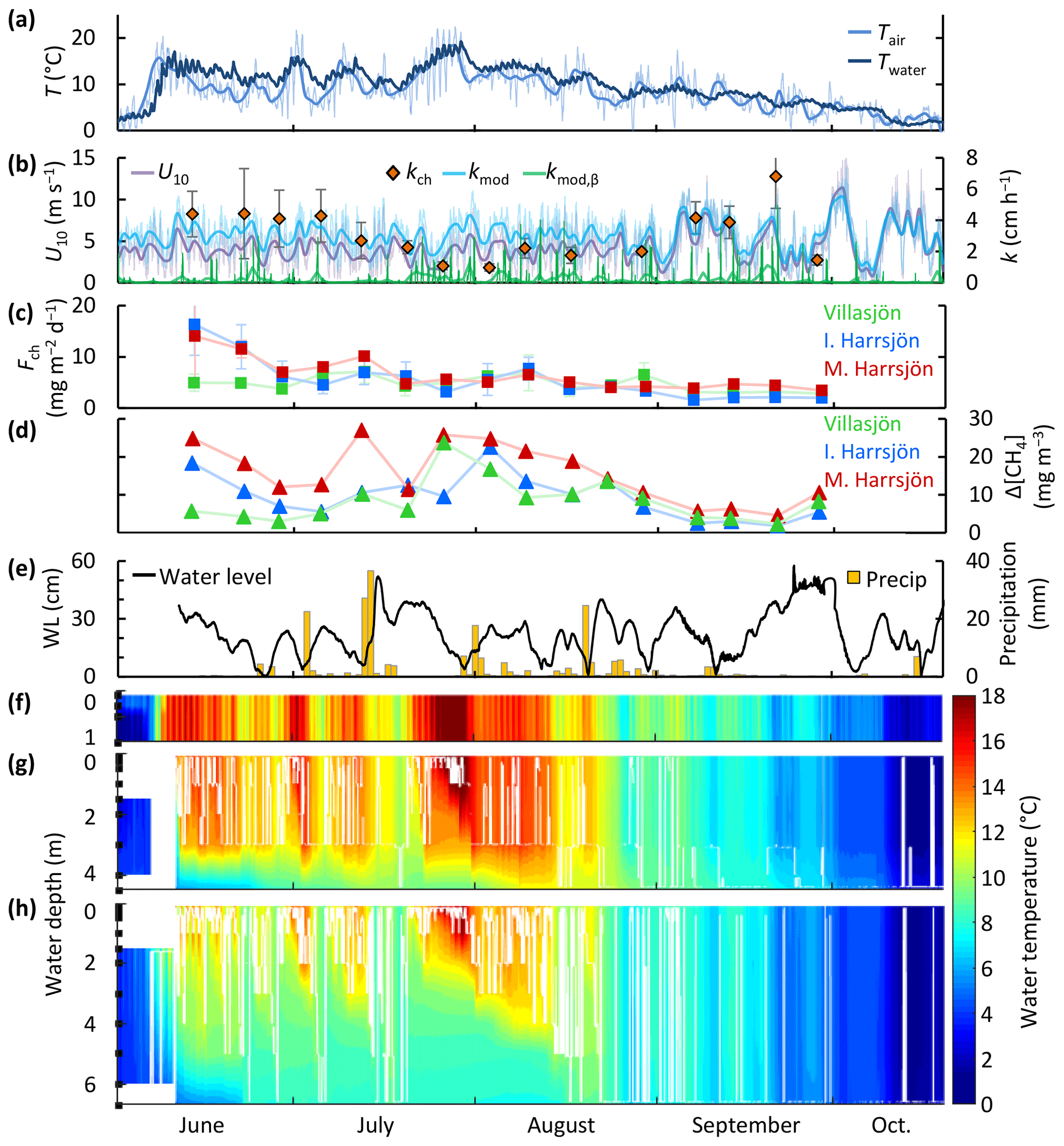
Figure 5 Time series of air and surface mixed-layer temperature (three-lake mean) (a), wind speed, gas transfer velocity from the surface renewal model (k_mod and its buoyancy component, k_mod,β) and from chamber observations (k_ch) (three-lake mean values, error bars represent 95 % confidence intervals) (b), chamber CH₄ flux (c), air–water CH₄ concentration difference (d), precipitation and changes in water level in Mellersta Harrsjön (e), and the water temperature in Villasjön (f), Inre Harrsjön (g), and Mellersta Harrsjön (h) during the ice-free season of 2017 (1 June to 20 October). The white lines in panels (f–h) represent the depth of the surface mixed layer. Thin and thick lines in panels (a) and (b) represent half-hourly and daily means, respectively. In panel (a) only the half-hourly time series of T_water was plotted.

3.3 CH₄ storage and residence times

Residence times of stored CH₄ varied between 12 h and 7 d and were inversely correlated with wind speed in all three lakes (OLS: R²≥0.57, Fig. 6). The mean residence time was shortest in the shallowest lake and was not significantly different between the two deeper lakes (paired t test, p<0.01, Table 3). We did not find a statistically significant linear correlation between the residence time and day of year or the water temperature. CH₄ storage was greatest in the deeper lakes and displayed patterns similar to the surface concentrations, increasing in the warmest months with water temperature and decreasing with wind speed.

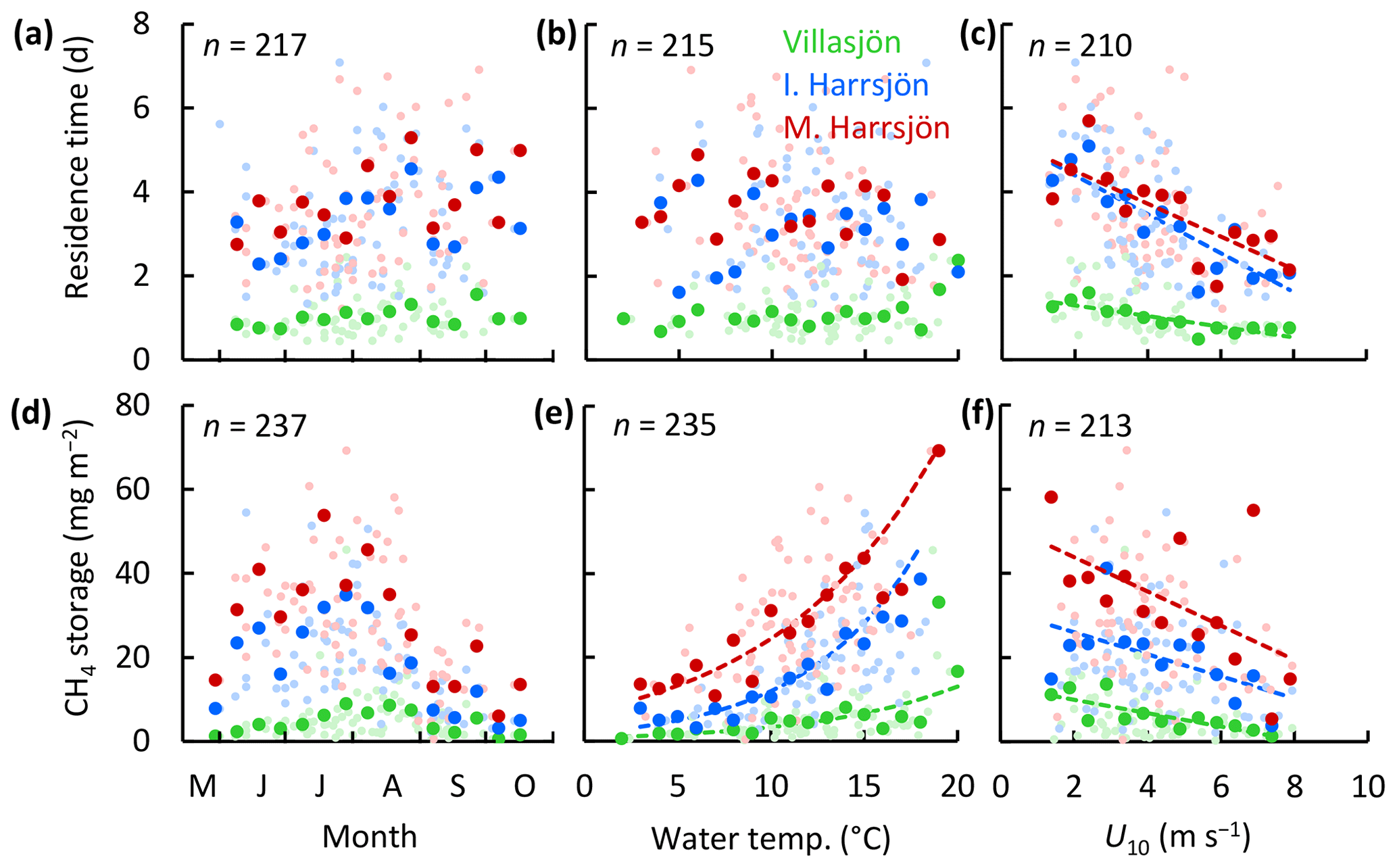
Figure 6 Scatter plots of the CH₄ residence time (a–c) and storage (d–f) versus time, surface water temperature, and wind speed. Symbol colours represent the different lakes. Large symbols represent binned means, and small symbols represent individual estimates. Bin sizes were 10 d, 1 ^∘C, and 0.5 m s⁻¹ for time, water temperature, and U₁₀, respectively. Each storage observation was paired with T and U₁₀ averaged over the 24 h (Villasjön) and 72 h (Inre and Mellersta Harrsjön) prior to water sampling, reflecting average conditions during CH₄ residence times. The linear regressions of the residence time onto time (a) and temperature (b) were not statistically significant (p=0.07–0.10). Linear relations of binned quantities and U₁₀ were statistically significant (c: p≤0.002; f: p≤0.04). Arrhenius-type functions (Eq. 7) adequately described the storage-temperature relation in each lake (e: R²≥0.70, p<0.001).

3.4 Variability

Chamber fluxes and surface water concentrations differed significantly between lakes (ANOVA, p<0.001, n=287, n=365) (Table 2). Both quantities were inversely correlated with lake surface area. CH₄ concentrations in the stream feeding the Mire (22.2±5.1 mg m⁻³, n=29, mean ±95 % CI) were significantly higher than those in the lakes (Table 2). Surface water concentrations over the deep parts of the deeper lakes (≥2 m water depth) were lower than those in the shallows (< 2 m) by 21 % to 26 % for Inre and Mellersta Harrsjön, respectively. However, the diffusive CH₄ flux did not differ significantly between depth zones in either Inre Harrsjön (ANOVA, p=0.27, n=290) or Mellersta Harrsjön (ANOVA, p=0.90, n=293) or between zones of high and low CH₄ ebullition in Villasjön (paired t test, p=0.27, n=89). The similar fluxes inshore and offshore present a contrast with ebullition, for which the highest fluxes were consistently observed in the shallow lake and littoral areas of the deeper lakes (Jansen et al., 2019; Wik et al., 2013).

Relations between the flux and its drivers – temperature, wind speed, and the surface concentration – manifested on different timescales (Fig. 7). Over the ice-free season both the CH₄ fluxes and surface water concentrations tracked changes in the water temperature. The wind speed (U₁₀) showed less variability over seasonal (CV = 7 %, n=17) than over diel timescales (CV = 12 %, n=24) and displayed a clear diurnal maximum. The surface water and sediment temperature varied primarily on a seasonal timescale (CV = 52 % and 45 %, n=17) and less on diel timescales (CV = 3 % and 2 %, n=24). Similar to the wind speed the gas transfer velocity varied primarily on diel timescales (Fig. 7), albeit with a lower amplitude. This was in part because $k_{\mathrm{mod}}\propto u^{\mathrm{3}/\mathrm{4}}$ (Eq. 4) and because the drag coefficient, used to compute the water-side friction velocity in Eq. 5, increases at lower wind speeds and under an unstable atmosphere, which was typically the case. The surface concentration was correlated with wind speed and temperature (Fig. 4f, g) and showed both seasonal and diel variability. On diel timescales Δ[CH₄] and k_mod were out of phase; Δ[CH₄] peaked just before noon, when the gas transfer velocity reached its maximum value (Fig. 7b, d). However, binned means of the 1 h chamber fluxes (F_ch (1 h)) were not significantly different at the 95 % confidence level (error bars) and did not show a clear diel pattern (Fig. 7b). Temporal patterns of fluxes and concentrations were very similar between the lakes (Figs. S2 and S3).

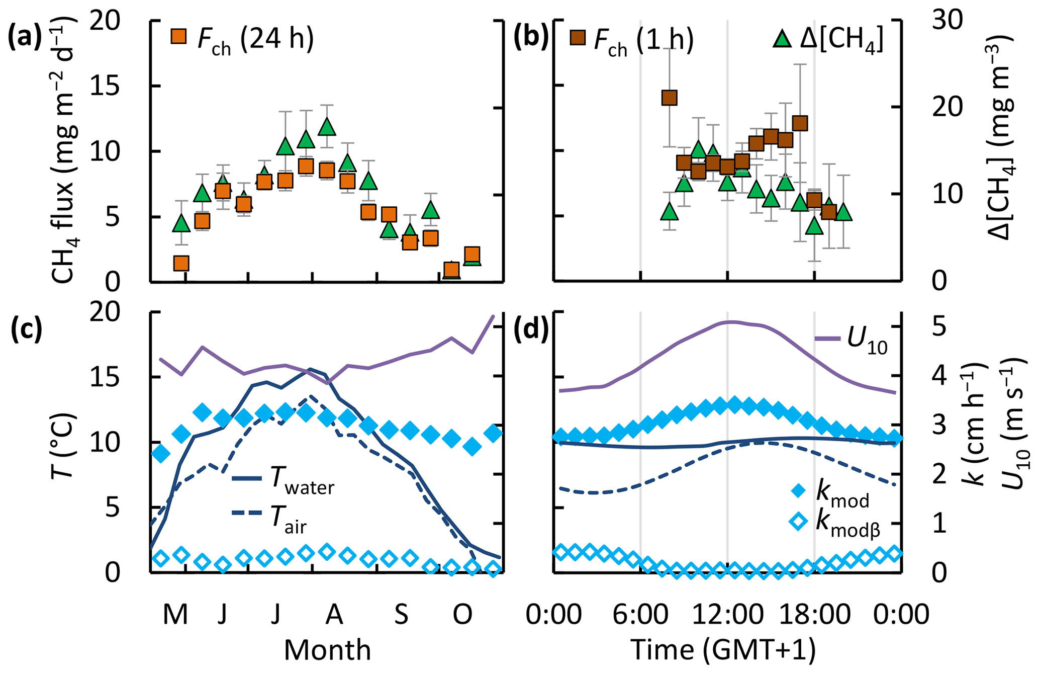
Figure 7 Temporal patterns of CH₄ chamber fluxes, concentrations (a, b), gas transfer velocity, air and surface water temperature, and wind speed (c, d). Bin sizes are 10 d (a, c) and 1 h (b, d). Error bars represent 95 % confidence intervals of the binned means. Temporal patterns in each individual lake are shown in Figs. S2 and S3.

3.5 Timescale analysis

The spectral density plot (Fig. 8a) disentangles dominant timescales of variability of the drivers of the flux. The power spectra of wind speed and temperature peaked at periods of 1 d and 1 year, following well-known diel and annual cycles of insolation and seasonal variations in climate (Baldocchi et al., 2001). The diel spectral peak was subdued for the surface sediment temperature. For U₁₀, the overall spectral density maximum between 1 d and 1 week, and somewhat longer in spectra for the ice-free period only (Fig. S4), corresponds to synoptic-scale weather variability, such as the passage of fronts (MacIntyre et al., 2009). U₁₀ and T_air also exhibit spectral density peaks at 1–3 weeks, which could be associated with persistent atmospheric blocking typical of the Scandinavian region (Tyrlis and Hoskins, 2008). While the temperature variability was concentrated at annual timescales, the wind speed varied primarily on timescales shorter than about a month and often shorter than a week.

The climacogram (Fig. 8b) reveals that the variability of the chamber flux and the gas transfer velocity were enveloped by that of the water temperature and the wind speed, as was the surface concentration difference for timescales < 5 months. The distribution of variability over the different timescales is similar to that shown in the spectral density plot (Fig. 8a). The standard deviation of the water temperature did not change from its initial value ($\mathit{\sigma }/{\mathit{\sigma }}_{\mathrm{init}}=\mathrm{1}$) until timescales of about 1 month, following the 1-year harmonic. In contrast, most of the variability of the wind speed was concentrated at timescales shorter than 1 month. The variability of the chamber and modelled fluxes first tracked that of the wind speed, but for timescales longer than about 1 month the decrease in variability resembled that of water temperature. The variability of the modelled fluxes followed that of the surface concentration difference rather than the gas transfer velocity. However, the coarse sampling resolution of the fluxes and concentrations may have led to an underestimation of both the variability at < 1-week timescales (Fig. 7b) and the value of σ_init. Finally, the climacogram shows that k_mod retains about 72 % of its variability at 24 h timescales, which justifies our averaging over chamber deployment periods for comparison with k_ch and the computation of the model scaling parameter α^′ (Fig. 3).

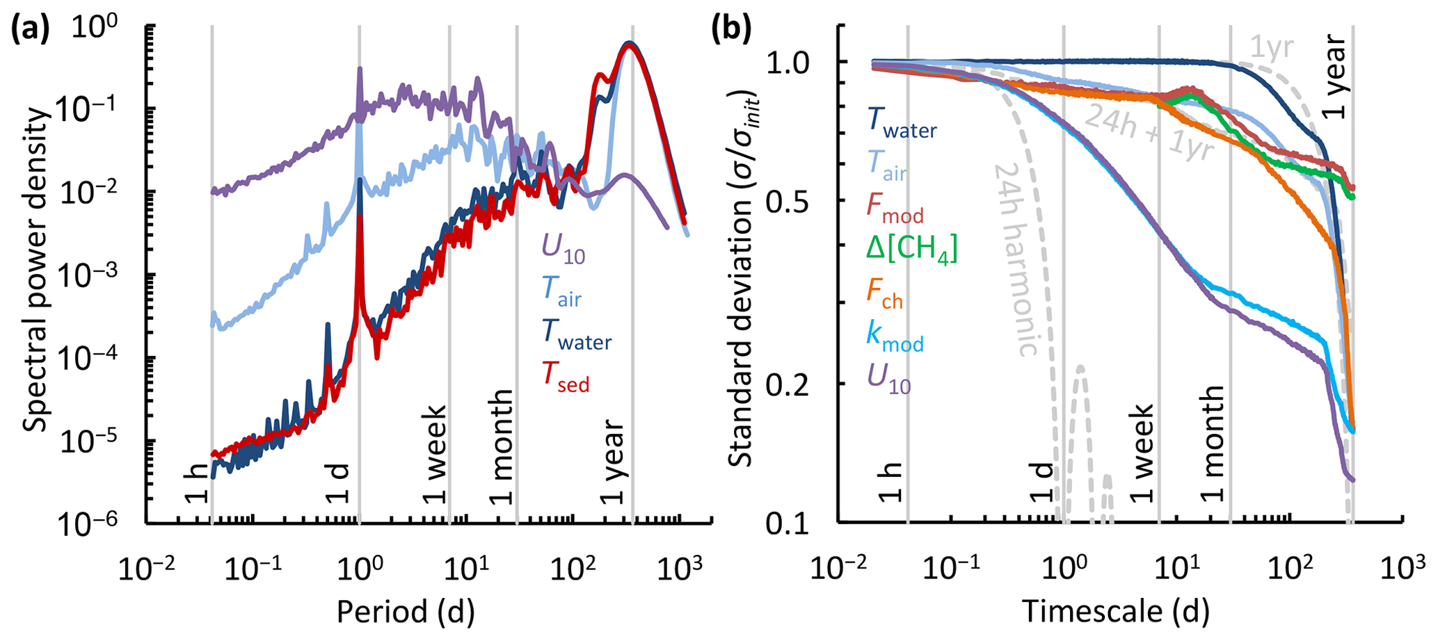
Figure 8 Timescale analysis of the diffusive CH₄ flux and its drivers. (a) Normalized spectral density of whole-year near-continuous time series of the air temperature (T_air), temperature of the surface water and ice (0.1–0.5 m, T_water), temperature of the surface sediment in Mellersta Harrsjön (T_sed), and wind speed (U₁₀). (b) Climacogram of the measured and modelled CH₄ flux (F_ch, F_mod), air and surface water temperature (T_air, T_water), water–air concentration difference (Δ[CH₄]), modelled gas transfer velocity (k_mod), and wind speed (U₁₀) during the ice-free seasons of 2009–2017. Dashed, light-grey curves represent (combinations of) trigonometric functions of mean 0 and amplitude 1 with a specified period. The 24 h and 1-year harmonic functions were continuous over the dataset period while the 24 h + 1-year harmonic was limited to periods when chamber flux data were available. Panel (a) is based on continuous time series that include the ice-cover seasons: Fig. S4 shows spectral density plots for individual ice-free seasons.

4 Discussion

4.1 Magnitudes of fluxes and gas transfer velocities

Overall, diffusive CH₄ emissions from the Stordalen Mire lakes (6.9±0.3 mg m⁻² d⁻¹, mean ±95 % CI) were lower than the average of postglacial lakes north of 50^∘ N, but within the interquartile range (mean 12.5, IQR 3.0–17.9 mg m⁻² d⁻¹; Wik et al., 2016b). Emissions are also at the lower end of the range for northern lakes of similar size (0.01–0.2 km²) (1–100 mg m⁻² d⁻¹; Wik et al., 2016b). As emissions of the Stordalen Mire lakes do not appear to be limited by substrate quality or quantity (Wik et al., 2018), but strongly depend on temperature (Fig. 4b), the difference is likely because a majority of flux measurements from other postglacial lakes were conducted in the warmer, subarctic boreal zone. Boreal lake CH₄ emissions are generally higher for lakes of similar size: 20–40 mg m⁻² d⁻¹ (binned means), n=91 (Rasilo et al., 2015) and ∼12 mg m⁻² d⁻¹, n=72 (Juutinen et al., 2009).

The gas transfer velocity in the Stordalen Mire lakes was similar to that predicted from wind-based models of Cole and Caraco (1998) and Crusius and Wanninkhof (2003) at low wind speeds (Fig. 9). Both were based on tracer experiments with sampling over several days and thus, like our approach, are integrative measures. The slope of the linear wind–k_ch relation (OLS: 0.81±0.21, slope ±95 % CI, R²=0.20 and p<0.01 for the individual k_ch estimates (small orange rhombuses in Fig. 9)) was similar to that reported by Soumis et al. (2008) (0.78 for a 0.06 km² lake), who also used a mass balance approach, and Vachon and Prairie (2013) (0.70–1.16 for lakes 0.01–0.15 km²). Part of the difference with the models of Vachon and Prairie (2013), Cole and Caraco (1998) and Soumis et al. (2008) was caused by the offset at 0 wind speed, which may stem from a larger contribution of the buoyancy flux in their lakes than we computed for our lakes with the surface renewal model (Crill et al., 1988; Read et al., 2012). The offset could also be caused by remnant wind shear turbulence (MacIntyre et al., 2018). While fetch limitation can reduce gas transfer at high wind speeds in small lakes (Vachon and Prairie, 2013; Wanninkhof, 1992), and the lakes studied here are at the low end of the size spectrum of water bodies in which the gas transfer models in Fig. 9 were developed (Table S1 in the Supplement), there are a number of other explanations for the low values we obtained. We further discuss these in Sect. 4.5 after evaluating drivers of flux.

4.2 Drivers of flux

Methane emitted from lakes in wetland environments can be produced in situ or be transported in from the surrounding landscape (Paytan et al., 2015). The distinction is important because some controls on terrestrial methane production, such as water table depth (Brown et al., 2014), are irrelevant in lakes. In the Stordalen Mire lakes, the Arrhenius-type relation of CH₄ fluxes and concentrations (Fig. 4b, f) together with short CH₄ residence times (Fig. 6) suggest that efficient redistribution of dissolved CH₄ strongly coupled emissions to sediment methane production. High CH₄ concentrations in the stream (Sect. 3.4) further suggest that external inputs of CH₄ – produced in the fens and transported into the stream with surface runoff, or produced in stream sediments – may have elevated emissions in Mellersta Harrsjön (Lundin et al., 2013). However, although the Mire exports substantial quantities of dissolved organic carbon (DOC) and presumably CH₄ from the waterlogged fens to the lakes (Olefeldt and Roulet, 2012), after rainy periods we observed either no significant change in Δ[CH₄] (3–6 July and 21–27 August 2017, Fig. 5) or a decrease (13–19 July 2017, Fig. 5). It remains unclear whether such reduced storage resulted from lower methanogenesis rates associated with the temperature drop after rainfall, convection-induced degassing, or lake water displacement or dilution by surface runoff.

Turbulent transfer was dominated by wind shear, and we computed a minor contribution (∼8 %) of the buoyancy-controlled fraction of k. Our result differs from that in Read et al. (2012), who found that buoyancy flux dominated turbulence production in temperate lakes 0.1 km² in size and smaller. For the Stordalen Mire lakes we computed higher ice-free season mean values of u_∗w, as well as lower values of the water-side vertical friction velocity, $w_{\ast w}=(\mathit{\beta }{z}_{\mathrm{mix}}{)}^{\mathrm{1}/\mathrm{3}}$, (1.2–1.8 mm s⁻¹) than they report (2.0–7.5 mm s⁻¹, n=40 lakes). The difference results from high wind speeds and often colder surface waters here compared to many temperate lakes. Therefore, values of sensible and latent heat fluxes are lower in our lakes than in lakes in warmer regions. Consequently, the temperate lakes surveyed in Read et al. (2012), will have a larger contribution of buoyancy flux to the gas transfer coefficient at night, when wind speeds are low (MacIntyre and Melack, 2009). The contribution of convection also depends on the wind-sheltering properties of the landscape surrounding the lake (Kankaala et al., 2013; Markfort et al., 2010). Depending on the turbulence environment, the buoyancy flux is thus weighed differently in different parameterizations of ε (Heiskanen et al., 2014; Tedford et al., 2014) and in wind-based models (offsets at U₁₀=0 in Fig. 9), contributing to significant divergence among model realizations of k (Dugan et al., 2016; Erkkilä et al., 2018; Schilder et al., 2016).

The distinct spectral peaks of temperature and U₁₀ (Fig. 8a) indicate that flux dependencies on these parameters (Fig. 4b, c) acted on different timescales. This difference has implications for the choice of models or proxies of the flux in predictive analyses. For lakes that mix frequently and have a climatology similar to that of the Stordalen Mire (Malmer et al., 2005), temperature-based proxies (e.g. Thornton et al., 2015) would resolve most of the variability of the ice-free diffusive CH₄ flux at timescales longer than a month. Advanced gas transfer models that account for atmospheric stability and rapid variations in wind shear, such as we have used here, allowed us to resolve variability in flux at timescales shorter than about a month. Our results are representative of small, wind-exposed lakes in cold environments, where, as a result of considerable wind driven mixing, fluxes are lower than would be predicted in lakes where buoyancy fluxes during heating and cooling are higher.

4.3 Storage and stability

The robust temperature sensitivity of lake methane emissions (Fig. 4b,f) (Wik et al., 2014; Yvon-Durocher et al., 2014) is driven by biotic and abiotic mechanisms. Lake mixing can modulate temperature relations by periodically decoupling production from emission rates (Engle and Melack, 2000). Here, enhanced CH₄ accumulation during periods of stratification may have contributed to concentration and storage maxima in July and August (Figs. 4e, 6d). However, as the CH₄ residence time was invariant over the season and with temperature (Fig. 6a, b), the storage–temperature relation (Fig. 6e) likely reflects rate changes in sediment methanogenesis rather than inhibited mixing. For example, the highest CH₄ concentrations in our dataset (59.1±26.4 mg m⁻³, n=37) were measured during a period with exceptionally high surface water temperatures ($T_{\mathrm{water}}=\mathrm{18.5}\pm \mathrm{3.6}$ ^∘C) that lasted from 23 June to 30 July 2014. Emissions during this period comprised 29 %–56 % (depending on the lake) of the 2014 ice-free diffusive flux, while the peak quantity of accumulated CH₄ comprised < 5 %. Two mechanisms may explain the lack of CH₄ accumulation. First, stratification was frequently disrupted by vertical mixing (Fig. 5g–h), and concurrent hypolimnetic CH₄ concentrations were not significantly different from (Inre Harrsjön, 2010–2017, paired t test, p=0.12, n=32) or lower than (Mellersta Harrsjön, 2010–2017, paired t test, p<0.01, n=35) those in the surface mixed layer. Second, stratification often was not strong enough to affect gas transfer velocities. Even when assuming ε was suppressed by an order of magnitude for N>25 and by 2 orders of magnitude for N>40 (MacIntyre et al., 2018), k_mod was only slightly lower (2.8 cm h⁻¹) than the multi-year mean (3.0 cm h⁻¹). Thus, in weakly stratified lakes with strong wind mixing, the temperature sensitivity of diffusive CH₄ emissions may be observed without significant modulation by stratification.

Degassing (Fig. 4c, g) prevented an unlimited increase in the emission rate with the gas transfer velocity. In this way, Δ[CH₄] acted as a negative feedback that maintained a quasi-steady state between CH₄ production and removal processes throughout the ice-free season. In all three lakes CH₄ residence times were inversely proportional to the wind speed (Fig. 6c), indicating an imbalance between production and removal processes. We hypothesize that the imbalance exists because the variability of wind speed peaked on shorter timescales than that of the water temperature (Fig. 8a). Changes in wind shear periodically pushed the system out of production–emission equilibrium, allowing for transient degassing and accumulation of dissolved CH₄. The temporal variability of dissolved gas concentrations is likely higher in shallow wind-exposed systems with limited buffer capacity (Natchimuthu et al., 2016, 2017) and should be taken into account when applying gas transfer models to small lakes and ponds.

Rapid degassing occurred at U₁₀≥6.5 m s⁻¹ (Fig. 4c). Gas fluxes at high wind speeds may have been enhanced by the kinetic action of breaking waves (Terray et al., 1996) or through microbubble-mediated transfer. Wave breaking was observed on the Stordalen lakes at wind speeds ≥7 m s⁻¹. Microbubbles of atmospheric gas (diameter < 1 mm) can form due to photosynthesis, rain, or wave breaking (Woolf and Thorpe, 1991) and remain entrained for several days (Turner, 1961). Due to their relatively large surface area, they quickly equilibrate with sparingly soluble gases in the water column, providing an efficient emission pathway to the atmosphere when the bubbles rise to the surface (Merlivat and Memery, 1983). In inland waters microbubble emissions of CH₄ have only been indirectly inferred from differences in CO₂ and CH₄ gas transfer velocities (McGinnis et al., 2015; Prairie and del Giorgio, 2013), and more work is needed to evaluate their significance in relatively sheltered systems.

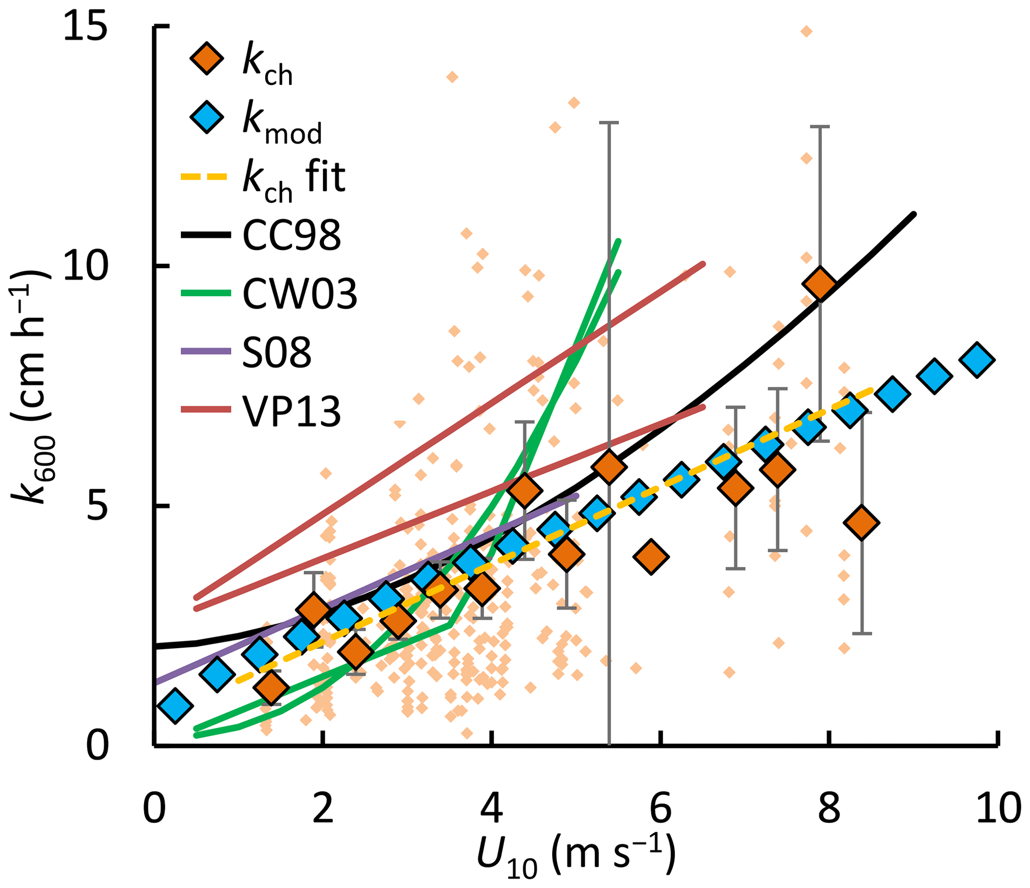
Figure 9 Normalized gas transfer velocities (k₆₀₀) versus the wind speed at 10 m (U₁₀). Binned values (large rhombuses, k_ch and k_mod, bin size = 0.5 m s⁻¹) and individual observations (small rhombuses, k_ch) from floating chambers (k_ch) and the surface renewal model (k_mod with ${\mathit{\alpha }}^{\prime }=\mathrm{0.23}$). Error bars represent 95 % confidence intervals of the binned means. Solid lines represent models from the literature: Cole and Caraco (1998) (CC98), Crusius and Wanninkhof (2003) (bilinear and power-law models) (CW03), Soumis et al. (2008) (S08) and Vachon and Prairie (2013) (VP13) for lake surface areas of 0.01 and 0.15 km². Supplement Table S1 lists the model equations and calibration ranges. A power-law regression model is shown for the individual k_ch datapoints (n=334): $k_{\mathrm{600}}=\mathrm{0.77}\times U_{\mathrm{10}}^{\mathrm{1.02}}+\mathrm{0.62}$ (dashed yellow line).

4.4 Timescales of variability

Overall, the short-term variability of the flux due to wind speed (1.1–13.2 mg m⁻² d⁻¹) was similar to the long-term variability due to temperature (0.7–12.2 mg m⁻² d⁻¹) (ranges of the binned means, Fig. 4b–c). The diel patterns in the mixed-layer depth (Fig. 5) and the gas transfer velocity (Fig. 7d) and daytime variation in the surface concentration (Fig. 7b) were indicative of daily storage-and-release cycles, resulting in a flux difference of about 5 mg m⁻² d⁻¹ between morning and afternoon, about half the mean seasonal range (Fig. 7a). Diel variability of lake methane fluxes has been observed at Villasjön (eddy covariance, Jammet et al., 2017) and elsewhere (Bastviken et al., 2004, 2010; Crill et al., 1988; Erkkilä et al., 2018; Eugster et al., 2011; Hamilton et al., 1994; Podgrajsek et al., 2014). Similarly, diel patterns in the gas transfer velocity have been inferred from eddy covariance observations (Podgrajsek et al., 2015) and in model studies (Erkkilä et al., 2018). Apparent offsets between the diurnal peaks of the flux, surface concentrations, and drivers (Fig. 7b, d) have been noted previously (Koebsch et al., 2015), but have yet to be explained. Continuous eddy covariance measurements in lakes where the dominant emission pathway is turbulence-driven diffusion could help characterize flux variability on short timescales (e.g. Bartosiewicz et al., 2015).

The CH₄ residence times (1–3 d) were not much longer than the diel timescale of vertical mixing (Fig. 5g, h). As a result, horizontal concentration gradients developed in the deeper lakes (Table 2). The 23±11 % concentration difference between depth zones in the deeper lakes (mean ±95 % Cl) fits transport model predictions of DelSontro et al. (2017) for small lakes (< 1 km²) that highlight the role of outgassing and oxidation during transport from production zones in the shallow littoral zones or the deeper sediments (Hofmann, 2013). Concentration gradients may also have been caused by physical processes, such as upwelling due to thermocline tilting (Heiskanen et al., 2014). Higher-resolution measurements, for example with automated equilibration systems (Erkkilä et al., 2018; Natchimuthu et al., 2016), are needed to assess how much of the spatial and diel patterns of the CH₄ concentration can be explained by physical drivers such as gas transfer and mixed-layer deepening (Eugster et al., 2003; Vachon et al., 2019), or by biological processes such as methanogenesis and microbial oxidation (Ford et al., 2002).

Gas transfer models can only deliver accurate fluxes if they are combined with measurements that capture the full spatio-temporal variability of the surface concentration (Erkkilä et al., 2018; Hofmann, 2013; Natchimuthu et al., 2016; Schilder et al., 2016). The short CH₄ residence times and diel pattern of Δ[CH₄] suggest that weekly sampling did not capture the full temporal variability of the surface concentrations. Especially after episodes of high wind speeds and lake degassing (Fig. 4c, g), concentrations may not have been representative of the 24 h chamber deployment period.

4.5 Model–chamber comparison

It is fundamental to our understanding of controls on fluxes to determine why empirically derived values of the model scaling parameter α^′ are relatively low in this study (0.17–0.31) compared to the theoretical value of $\sqrt{\mathrm{2}/\mathrm{15}}\cong \mathrm{0.37}$ (Katul et al., 2018) and why they were different among the three lakes. k_mod did not differ significantly between lakes (ANOVA, p<0.001), and therefore differences in α^′ resulted from diverging k_ch values estimated at 3.5±0.7 (n=74), 3.1±0.4 (n=131) and 2.5±0.6 (n=142) cm h⁻¹ in Villasjön, Inre Harrsjön, and Mellersta Harrsjön, respectively (mean ±95 % CI). Synthesis studies show that scaling parameter values can vary between 0.1 and 0.7 over the range of moderate to high dissipation rates computed for the Stordalen Mire lakes (Eq. 5: $\mathit{\epsilon }={\mathrm{10}}^{-\mathrm{7}}$–10⁻⁵ m² s⁻³) (Esters et al., 2017; Wang et al., 2015, and references therein). In such cases ε has been measured directly with acoustic Doppler or particle image velocimetry and compared with independent estimates of k using chambers (Gålfalk et al., 2013; Tokoro et al., 2008; Vachon et al., 2010; Wang et al., 2015), eddy covariance observations (Heiskanen et al., 2014), or the gradient flux technique (Zappa et al., 2007) and a sparingly soluble tracer, such as CO₂ or SF₆. Measured and modelled lake CO₂ fluxes agree reasonably well if Eqs. (4) and (5) are used with a multi-study mean α^′ of 0.5 (Bartosiewicz et al., 2015; Czikowsky et al., 2018; Erkkilä et al., 2018; Mammarella et al., 2015), but the agreement is less clear for CH₄ fluxes (Bartosiewicz et al., 2015). The observed variability in α^′ could be explained by chemical or biological factors that limit surface exchange or by the variable contributions of wind sheltering, atmospheric stability, and within-lake stratification and mixing. Here, the low α^′ value may imply an underestimation of k derived from chamber observations or an overestimation of dissipation rates used in the modelling of gas transfer velocities.

An underestimation of chamber-derived gas transfer velocities may have resulted from an overestimation of C_aq in Eq. (1). This can occur if significant methane oxidation takes place at the air–water interface. This additional removal process would invalidate the implicit assumption in Eqs. (1) and (2) that the dissolved CH₄ concentration measured in the bulk fluid is representative of the concentration in the diffusive sublayer. Omitting oxidation would bias Δ[CH₄] high and k_ch low. Laboratory gas exchange experiments have demonstrated methanotrophy in the ∼1 µm thick surface microbiome (bacterioneuston) of seawater (Upstill-Goddard et al., 2003). While we are not aware of similar experiments in freshwater, CH₄ oxidation is ubiquitous in northern lakes and can be substantial even in the epilimnion (Martinez-Cruz et al., 2015, Thottathil et al., 2018). The Stordalen Mire lakes remained oxygenated throughout the ice-free season and CH₄ stable isotopes indicate that between 24 % (Villasjön) and 60 % (Inre and Mellersta Harrsjön) of CH₄ in the water column was continually oxidized (Jansen et al., 2019). This may explain not only the low scaling parameter value compared to those found with other tracers, but also why α^′ was higher in Villasjön (0.31, n=67) than in the deeper lakes (0.17–0.25, n=267) (Fig. S1). However, more work is needed to establish how methanotrophy is partitioned between the air–water interface, where it would affect estimation of k, and the deeper water column and sediment. An increase in surface concentrations which typically occurs at night would not have been manifest (Crill et al., 1988; Czikowsky et al., 2018) because there was, apart from the period just after thaw of the ice cover in 2017, no significant CH₄ accumulation below the mixing layer throughout the ice-free seasons. Indeed, CH₄ concentrations within the 0.1–1 m surface layer of the deeper lakes (Table 2) were not significantly different from those at greater depth (Inre Harrsjön: 12.2±2.7 mg m⁻³, n=292; Mellersta Harrsjön: 17.7±4.9 mg m⁻³, n=405; means ±95 % CI).

An overestimation of gas transfer velocities computed with the surface renewal model may result if actual dissipation rates are lower than we compute. This occurs under high wind shear when more of the introduced turbulent kinetic energy is used for mixing the water column and deepening the mixing layer and less is dissipated (Ivey and Imberger, 1991; Jonas et al., 2003). When this occurs, the coefficient on $u_{\ast w}^{\mathrm{3}}$ in Eq. (5) may have a lower value (Tedford et al., 2014), which translates to a reduced estimate of ε and increased α^′ values. A similar decrease in ε can be assumed during heating, when strong stratification (N>25 cph) dampens turbulence dissipation (MacIntyre et al., 2010, 2018); however, such stratification was intermittent in our study (Fig. 5f–h).

Reduced gas transfer velocities and between-lake differences in k_ch could also be due to differences in atmospheric forcing. First, the wind speed may have been lower over the lakes than on the Mire due to the slight elevation (< 1 m) of the surrounding peatland hummocks (Markfort et al., 2010). The wind-sheltering effect of tall shrubs (Betula nana L; Malmer et al., 2005) on the shores of the deeper lakes (Fig. 1) was readily noticed during sample collection, particularly in Mellersta Harrsjön. Second, atmospheric stability was different over the three lakes. The atmosphere was stable ($z/L_{\mathrm{MO},\mathrm{a}}\mathit{>}\mathrm{0}$) over Mellersta Harrsjön, Inre Harrsjön, and Villasjön during 29 %, 21 %, and 22 % of the ice-free periods (2009–2017), respectively, with drag coefficients ∼16 % lower than their neutral value during these times. The effect was more pronounced when winds were light during daytime heating, with somewhat higher frequency during autumn. Colder incoming stream water flowing into Mellersta Harrsjön may have contributed to lower surface water temperatures in this lake (Table 3), with the discrepancy more noticeable as lake level rose (Fig. 5e–h). More frequent periods with a stable atmosphere above Mellersta Harrsjön reduced sensible and latent heat fluxes and are a likely cause of the increased stratification of the surface layer: water at 0.1 m was sometimes 0.5 to 2 ^∘C warmer than at 0.3 m in Mellersta Harrsjön (5 % of the time during ice-free seasons) when temperatures were isothermal in the upper 0.5 m in Villasjön and Inre Harrsjön. Greater near-surface stratification coupled with lower winds than measured on the Mire would have led to the lower values of k and α^′ obtained in this lake. While this analysis points to the challenges in modelling fluxes when meteorological instrumentation is not situated on the lakes, it also suggests that a solution is to use lower values of α^′ when modelling k for sheltered water bodies.

In summary, the model scaling parameter α^′ computed in this study is lower than the theoretical value of 0.37 and 0.5 recently obtained in eddy covariance studies in which CO₂ fluxes were measured and modelled. The discrepancy may be explained by surface CH₄ concentrations decreasing due to microbial oxidation over the same timescale as our chamber measurements. Alternate explanations take into account the magnitude of wind shear and degree of sheltering. Differences in α^′ between lakes indicate the care required in modelling emissions from sheltered lakes; the overall cooler surface water temperatures in the lake with greater stream inflows point to a new control on emissions. That is, when stream inflows lead to surface water temperatures cooler than air temperature in sheltered lakes, a stable atmosphere results, which leads to a reduced momentum flux, lower emissions, and a longer time over which methane oxidation can occur. The cooling effect may be especially pronounced in northern landscapes underlain by permafrost, where the temperature of meltwater streams and subsurface flow in the active layer remain low throughout the year. Thus, these comparisons of modelled and measured fluxes point to new areas of research.

5 Summary and conclusions

In this study we combined a unique, multi-year dataset with a modelling approach to better understand environmental controls on turbulence-driven diffusion-limited CH₄ emissions from small, shallow lakes. Floating chambers estimated the seasonal mean flux at 6.9 mg m⁻² d⁻¹ and illustrated how the flux depended on temperature and wind speed. Wind shear controlled the gas transfer velocity while thermal convection and release from storage were minor drivers of the flux. CH₄ fluxes and surface concentrations fitted an Arrhenius-type temperature function ($E_{\mathrm{a}}^{\prime }=\mathrm{0.88}$–0.97 eV), suggesting that emissions were strongly coupled to rates of methanogenesis in the sediment. However, temperature was only an accurate proxy of the flux on averaging timescales longer than a month. On shorter timescales, wind-induced variability in the gas transfer velocity, mixing-layer depth, and storage decoupled production from emission rates. Transient changes in the lake mixing regime allowed for periodic CH₄ accumulation and resulted in an inverse relationship between wind speed and surface concentrations. In this way, the air–water concentration difference acted as a negative feedback to emissions and prevented complete degassing of the lakes, except at high wind speeds (U₁₀≥6.5 m s⁻¹).

Freshwater flux studies are increasingly focused on understanding mechanisms and developing proxies for use in upscaling efforts and process-based models. Simple temperature- or wind-based proxies can yield accurate flux estimates, but model parameters, such as $E_{\mathrm{a}}^{\prime }$ and α^′, must be calibrated to local conditions to reflect relevant biotic and abiotic processes at appropriate timescales. Our study highlights the importance of non-linear feedbacks, such as shallow lake degassing at high wind speeds, as well as microbial removal processes and the need to consider the timescale over which fluxes occur relative to the timescale over which CH₄ can be oxidized. More work is needed to quantify the importance of microbial removal processes at the air–water interface of freshwater ecosystems. Advanced gas transfer models can only improve the accuracy of flux estimates if they are paired with observations that capture the meteorological conditions over the lake and the spatio-temporal variability of dissolved gas concentrations. Therefore, field measurements remain necessary to inform, calibrate, and validate models. Our results indicate that the timescale of driver variability can inform the frequency of field measurements necessary to yield representative datasets for novel proxy development.