the Creative Commons Attribution 4.0 License.
the Creative Commons Attribution 4.0 License.
 | 29 May 2020
Wind-driven stratification patterns and dissolved oxygen depletion off the Changjiang (Yangtze) Estuary
Taavi Liblik
Yijing Wu
Daidu Fan
Dinghui Shang
Multiple factors have been accused of triggering coastal hypoxia off the Changjiang Estuary, and their interactions lead to high yearly variation in hypoxia development time window and distribution extent.
Two oceanographic cruises, conducted in July 2015 and August–September 2017, were complemented by river discharge, circulation simulation, remotely sensed wind, salinity and sea level anomaly data to study the dissolved oxygen (DO) depletion off the Changjiang Estuary from synoptic to interannual timescales. Intensification of the Chinese Coastal Current and Changjiang Diluted Water (CDW) spreading to the south together with coastal downwelling caused by the northerly wind was observed in the summer of 2015. This physical forcing led to a well-ventilated area in the north and a hypoxic area of 1.3×10⁴ km2 in the south, while in 2017 the summer monsoon (southerly winds) induced offshore transport in the surface layer that caused a subsurface intrusion of Kuroshio-derived water to the shallower areas (<10 m depth) in the north and upwelling in the south. Wind-driven Ekman surface flow and reversal of the geostrophic current related to the upwelling compelled alteration of the Chinese Coastal Current. Consequently, intense hypoxia (DO down to 0.6 mg L−1) starting from 4 to 8 m depth connected to CDW and deep water intrusion in the north and coastal hypoxia linked to the upwelling in the south were observed in 2017.
Distinct situations of stratification and DO distributions can be explained by wind forcing and concurrent features in surface and deep layer circulation, upwelling and downwelling events. Enhanced primary production in the upper layer of the CDW or the upwelled water determines the location and extent of DO depletion. Likewise, the pycnocline created by Kuroshio subsurface water intrusion is an essential precondition for hypoxia formation.
Wind forcing largely controls the interannual change of hypoxic area location and extent. If the summer monsoon prevails, extensive hypoxia more likely occurs in the north. Hypoxia in the south occurs if the summer monsoon is considerably weaker than the long-term mean.
- Article
(18187 KB) - Full-text XML
-
Supplement
(67 KB) - BibTeX
- EndNote


Dead zones in the coastal ocean have spread since the 1960s (Diaz and Rosenberg, 2008). Besides eutrophication (Diaz and Rosenberg, 2008), climate change (Altieri and Gedan, 2015) intensifies dissolved oxygen (DO) depletion. Estuaries and other regions of freshwater influence are typically very productive areas and often experience hypoxia (Conley et al., 2009; Cui et al., 2019; Obenour et al., 2013; Testa and Kemp, 2014). Hypoxia is a condition of low DO, which cannot be sustained by marine life. Depending on marine organisms, hypoxia can have various definitions (Vaquer-Sunyer and Duarte, 2008). In the present study, hypoxia is defined as a DO concentration of <3.0 mg L−1. Natural and anthropogenic nutrient load in these areas leads to intensive sedimentation of organic matter. DO is used by concurrent decomposition of detritus by bacteria in the subsurface layer. The deep layer below the euphotic zone can receive DO by physical processes only – lateral advection and vertical mixing. If the decline of DO exceeds DO import or production, the DO concentrations decrease.
Hypoxia is a natural phenomenon in the East China Sea (ECS) off the Changjiang Estuary, as evidence of its existence extends back to 2600 years at least (Ren et al., 2019). However, the hypoxic area has been expanding in recent decades (Chen et al., 2017; Ning et al., 2011; Zhu et al., 2011), which can be mostly related to eutrophication (Wang et al., 2016). A low-DO zone off the estuary can be found from late spring (Zuo et al., 2019) until autumn when stratification decays (Wang et al., 2012). The formation and maintenance of seasonal hypoxia have been related to various physical, biogeochemical and biological processes such as vertical mixing and eutrophication (Ning et al., 2011). Hypoxia off the Changjiang Estuary is in the literature often divided into the areas north and south of 30∘ N (Wei et al., 2017a; Zhu et al., 2011). The northern part features a shallow (20–40 m) and flat sea bottom, while the southern part is characterized by a deep trough with water depth >60 m and a steep slope. Numerous small peninsulas and islands occupy the southern part with irregular coastline.
The region is strongly impacted by huge discharge from the Changjiang (Yangtze) River (Beardsley et al., 1985; Xu et al., 2018). Correlation between the Changjiang Diluted Water (CDW) plume area and river discharge has been suggested by Kang et al. (2013). Nutrient-rich freshwater mixes with ocean water to form the CDW. Enhanced primary production in the CDW causes intense detritus accumulation and DO consumption in the near-bottom layer (Chen et al., 2017; Große et al., 2019; Z. Li et al., 2018; Wang et al., 2017, 2016; Zhou et al., 2019). The CDW is separated from the deeper water by a shallow halocline, which often coincides with the seasonal thermocline (Zhu et al., 2016). The shallow pycnocline impedes vertical mixing and consequently DO transport downwards. Thus, the presence of the CDW provides favorable conditions for hypoxia formation in the layer below the pycnocline. Moreover, the shallow pycnocline supports accelerated warming in summer (Moon et al., 2019), which in turn strengthens the pycnocline even more. Therefore, the spreading of the CDW strongly determines oxygen depletion in the near-bottom layer.
Shallower areas near the river mouth are strongly impacted by tidal forcing (L. Li et al., 2018). However, in the open sea, the contribution of tides in the vertical mixing budget is low compared to that of wind stirring (Ni et al., 2016). Abrupt wind mixing events can weaken stratification and considerably increase DO concentrations in the deep layer (Ni et al., 2016). However, such vertical mixing also causes the nutrient flux to the upper layer (Hung et al., 2013), consequently enhancing primary production in the upper layer and then DO consumption in the deep layer (Ni et al., 2016).
Besides the CDW and wind mixing, circulation and hydrography near the Changjiang Estuary are further influenced by the Chinese Coastal Current and the Taiwan Warm Current. The latter originates from the Taiwan Strait warm water (>25 ∘C; e.g., J. Zhang et al., 2007) at the surface and the shelf-intrusion water of Kuroshio subsurface water (KSSW, <25 ∘C; e.g., J. Zhang et al., 2007) at the bottom (Lie and Cho, 2002, 2016; Liu et al., 2017; L. Zhang et al., 2007; Zuo et al., 2019). Geostrophic currents in the area are modified by wind forcing, which exhibits seasonal alternation of winter and summer monsoons (Lie and Cho, 2002). Winds from the north and northeast prevail during the winter monsoon, and southerly winds dominate during the summer monsoon (Chu et al., 2005). The summer monsoon favors upwelling in the ECS (Hu and Wang, 2016), including the offshore area near the Changjiang Estuary (Xu et al., 2017; Yang et al., 2019). Upwelling events bring large amounts of nutrients to the surface layer (Wang and Wang, 2007), which cause an increase in primary production and a subsequent decrease in DO concentrations in the near-bottom layer (Chen et al., 2004; Zhou et al., 2019). Moreover, coupling of the CDW plume and upwelled KSSW has an effect on primary production and hypoxia formation in the near-bottom layer (Wei et al., 2017a). CDW spreading and upwelling of subsurface water are both sensitive to wind forcing, which gives rise to the hypothesis that hypoxic conditions are strongly dependent on wind conditions.
Zhang et al. (2018) demonstrated that high mobility of the CDW strongly controls the variation of location and areal extent of bottom hypoxia. Thus, distributions of oceanographic fields mapped during an occasional research cruise could depend on simultaneous synoptic-scale forcing conditions and do not necessarily represent the hydrographical and chemical situation in a particular summer. In order to put oceanographic cruise results in a more general context, observed ocean variables must be linked to the forcing. The role of nutrient consumption and primary production in the CDW and the upwelled water and their interaction have been previously investigated. Enhanced primary production due to upwelling and the CDW spreading produces higher oxygen consumption rates in the near-bottom layer (Chen et al., 2017, 2004; Große et al., 2019; Z. Li et al., 2018; Wang et al., 2017, 2016; Wei et al., 2017a; Zhou et al., 2019). The focus of this work will be on the physical forcing mechanisms that create favorable conditions for the formation and maintenance of hypoxia.
We hypothesize that prevalent physical factors, wind forcing and river runoff, mainly determine the stratification patterns and, consequently, the location and areal extent of the DO depletion off the Changjiang Estuary. That is, changes in forcing over various timescales (synoptic, interannual and decadal) cause changes in the patterns of stratification and bottom hypoxia. To test this hypothesis, we (1) describe spatial patterns of temperature, salinity, chlorophyll a (Chl a) and DO off the Changjiang Estuary during two cruises in the summers of 2015 and 2017; (2) explore the potential links between physical variables and DO distributions; and (3) investigate the forcing mechanism behind the observed patterns.
We performed two surveys in the Changjiang Estuary and the adjacent sea on board the RV Zhehaike-1 from 27 August to 5 September 2015 and from 24 to 29 July 2017, respectively. CTD (conductivity, temperature and depth) and DO profiles were obtained from 110 stations in 2015 and 83 stations in 2017. However, we have excluded stations inside the estuary; therefore, 65 and 49 stations were included in the present study in 2015 and 2017, respectively (Fig. 1). At all stations, vertical profiles of temperature, salinity and DO were recorded with the SBE 25plus Sealogger CTD with DO sensor SBE 43. The DO sensor was calibrated against water sample analyses conducted by the Winkler titration method. Linear regressions between sensor and sample DO concentration data for 2015 and 2017 were analyzed: (r2=0.93, n=191) and (r2=0.99, n=98), where DOSBE is the DO concentration recorded by the SBE 43 sensor (Wu et al., 2019). Survey data is given in the Supplement.
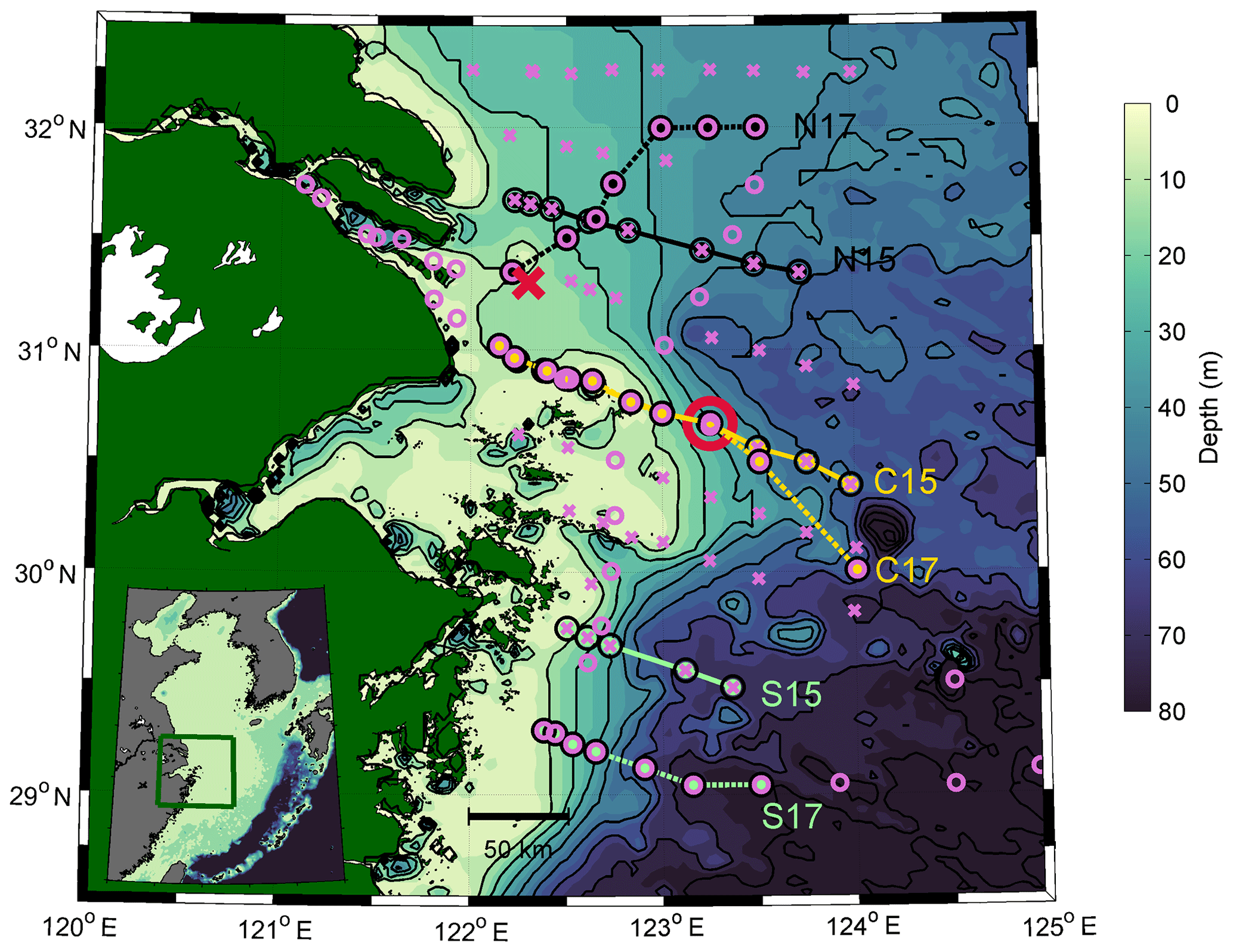
Figure 1Map of the study area off the Changjiang Estuary. Crosses represent CTD cast stations conducted on 27 August–5 September 2015 and circles show CTD cast stations on 24–29 July 2017. Lines represent northern sections (N15 in 2015 and N17 in 2017), central sections (C15 in 2015 and C17 in 2017), and southern sections (S15 in 2015 and S17 in 2017). The larger circle represents the mooring M1 location. The larger cross shows the location, where wind data were gathered. The color scale shows depth (m) of the study area. The inlay shows the study area in the East China Sea.
For the 2015 cruise, Chl a concentrations were measured from water samples as follows. About 500 mL surface water was filtered through 0.7 µm (pore size) Whatman glass fiber filters at every station with pressure lower than 15 kPa to get the particles for further analysis. To avoid the influence of light during the storage, all filters after filtration were folded up and wrapped by the aluminum foil before being preserved in the −20∘ freezer. The pigments in each filter were extracted by 90 % acetone and measured by fluorometric analysis using the Hitachi fluorescence spectrophotometer (F-2700).
Since in situ Chl a was not sampled in 2017, the daily satellite (Aqua MODIS) derived Chl a data were downloaded from https://coastwatch.pfeg.noaa.gov/ (last access: 11 April 2018). According to data availability, a mean Chl a field on 21–22 July, i.e., 3–4 d before our survey, was presented to illustrate primary production in 2017.
Salinity data in the present work are given in the Practical Salinity Scale (Fofonoff and Millard, 1983) and density as potential density anomaly (σ0) to a reference pressure of 0 dbar (Association for the Physical Sciences of the Sea, 2010).
The 8 d running average Sea Surface Salinity (SSS) data with a resolution of 0.25∘ calculated from the Soil Moisture Active Passive (SMAP) mission (Meissner et al., 2018) were used to estimate the spatial extent of CDW from 2015 to 2018. Remotely sensed salinity agreed with the in situ salinity measurements (Fig. 2) at the mooring station M1 (Fig. 1).

Figure 2Time series of in situ and remotely sensed 8 d running mean salinity at the M1 location in 2017.
Reprocessed 6-hourly wind observations with a horizontal resolution of 0.25∘ from 1993 to 2018 downloaded from the Copernicus Marine Service (product ID WIND_GLO_WIND_L4_REP_ OBSERVATIONS_012_006, http://marine.copernicus.eu/, last access: 16 May 2019) were used to describe wind conditions. Wind stress was calculated following Large and Pond (1981):
where ρair is the air density, CD is the drag coefficient, and U10 is the wind speed at the reference height of 10 m above sea level.
Current speed and direction from 1993 to 2018 were downloaded from the Copernicus Marine Service reanalysis product GLORYS12V1. The global eddy-resolving model has a regular horizontal grid of approximately 8 km (1∕12∘) and standard vertical levels with resolutions increasing from 1 m near the surface to 8 m around 50 m depth and then to 17 m around 100 m depth. Remotely sensed and observed in situ temperature, salinity and sea level were assimilated to the model. The model has too coarse a resolution to estimate details of meso- and finer-scale features in the area. However, it can be used to estimate the general current patterns.
Daily mean sea level anomaly and meridional and zonal components of absolute geostrophic velocity based on satellite altimetry were downloaded from the Copernicus Marine Service (product DATASET-DUACS-REP-GLOBAL-MERGED-ALLSAT-PHY-L4). The sea level anomaly is defined as the sea surface height above the mean sea surface during the reference period 1993–2012. The horizontal and temporal resolution of the dataset is 0.25∘ and 1 d, respectively.
To estimate oxygen consumption, the apparent oxygen utilization (AOU) between DO concentration at the saturation level and measured DO concentration in water with the same temperature and salinity was calculated as follows:
where DOS is DO concentration at the saturation level (Weiss, 1970) and DOM is the measured DO concentration. Total AOU (g m−2) in the water column was calculated as
where AOU(z) is the AOU profile and h is the water column depth.
The upper boundary of the DO depletion was defined as the AOU isoline 2 mg L−1. The 2 mg L−1 criterion was visually chosen from the AOU profiles in order to describe the center of the oxycline. Different authors have used various criteria (Lie and Cho, 2002; Liu et al., 2017; J. Zhang et al., 2007; L. Zhang et al., 2007; Zuo et al., 2019) to define water masses in the region. The cold bottom water in the area mostly originates from the KSSW (Liu et al., 2017). Therefore, we define deep layer water as the upper boundary of the KSSW by the isotherm 24.5 ∘C (J. Zhang et al., 2007).
Daily (2015 and 2017 summer) and monthly (2001–2018) river discharge data from Datong hydrological station (see location in Xu et al., 2018) were used in this study.
The width of the buoyant coastal current was estimated according to Lentz and Helfrich (2002):
where f is the Coriolis force, Q is the volume transport (taken as river discharge), g is the gravitational acceleration, dρ is the density difference between the plume and ambient fluids (ρ), and α is the coastal slope.
3.1 Spatial patterns of hydrography, chlorophyll a and oxygen in 2015 and 2017
In order to link the thermohaline structure and DO observations, we analyzed temperature, salinity, stratification and DO distributions observed in the summers 2015 and 2017. To explore the relationship between primary production and subsequent organic matter degradation and oxygen depletion, distributions of Chl a and AOU were compared.
The water of SSS<30 was observed along the coastal zone of the entire study area in 2015 (Fig. 3a). The 25 isohaline reached 29.3∘ N in the southern part of the study area, while its northern boundary was at 31.7∘ N near the mouth of the Changjiang Estuary in 2015. In 2017, the 25 isohaline reached only 30.6∘ N in the southern part of the study area (Fig. 3b), and the water fresher than 25 was also observed in the east and northeast of the Changjiang Estuary. Thus, the southward-spreading CDW was indicated to prevail before the survey in 2015, but the eastern and northeastern diversion of CDW was prevalent before the survey in 2017.
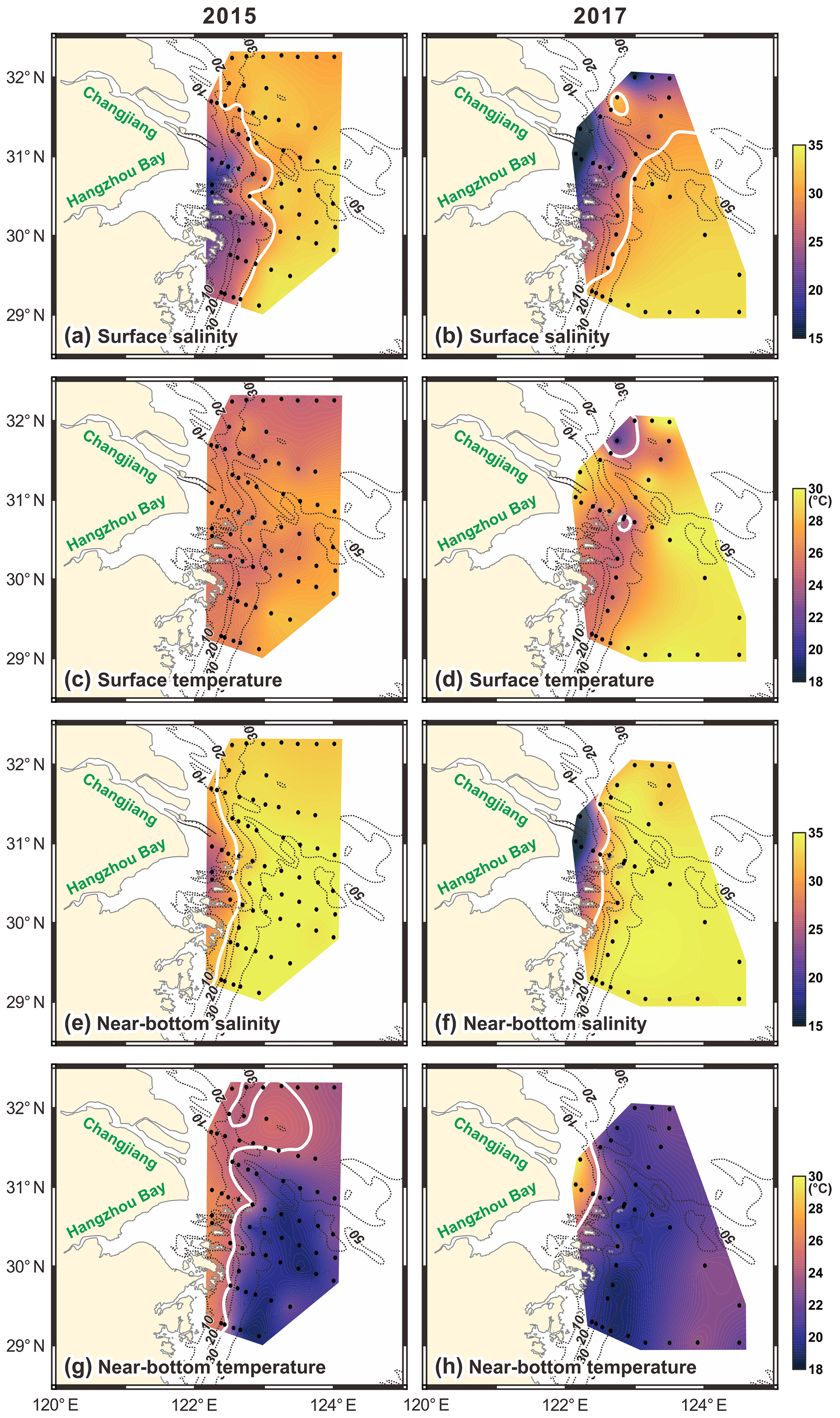
Figure 3Maps of surface salinity (a, b), surface temperature (c, d), near-bottom salinity (e, f) and near-bottom temperature (g, h) from the surveys in 2015 (a, c, e, g) and 2017 (b, d, f, h). The 30 and 24.5 ∘C isolines are shown as white lines.
Colder surface water was observed along the coast between 28.5 and 31∘ N, as well as in the northern part of the study area (>31.5∘ N) in both years. The sea surface temperature (SST) was much lower in these regions, but colder water covered smaller areas in 2017 (Fig. 3d) than in 2015.
The near-bottom temperature difference between the two surveys was particularly large in the northern part of the study area (Figs. 3g–h, 4a, 5a). The near-bottom temperature was 24–25 ∘C in 20–30 m water depth in 2015 (Fig. 4a), while it was 21–22 ∘C in 2017 (Fig. 5a). Likewise, near-bottom water was much saltier in 2017 than in 2015 (Figs. 3e–f, 4d, 5d). The minimum near-bottom temperature zone was located at 50–60 m water depth in the southern and central part of the study area in 2015 (Figs. 3g and 4b–c), but it shifted onshore to much shallower depths in 2017 (Figs. 3h and 5a–c).

Figure 4Vertical distributions of temperature, salinity, density, DO concentration and apparent oxygen utilization (AOU) along sections N15, C15 and S15 in 2015 (Fig. 1). Temperature isoline 24.5 ∘C is shown with the thicker dashed line in the temperature, oxygen and AOU plots. AOU isoline 2 mg L−1 is shown with the thicker solid line in AOU plots. The hypoxia border (3.0 mg L−1) is shown with a thicker solid line in oxygen plots. Locations of CTD stations are shown as crosses in the top panels. Values on the x axis indicate the distance from the westernmost point of a section (Fig. 1).
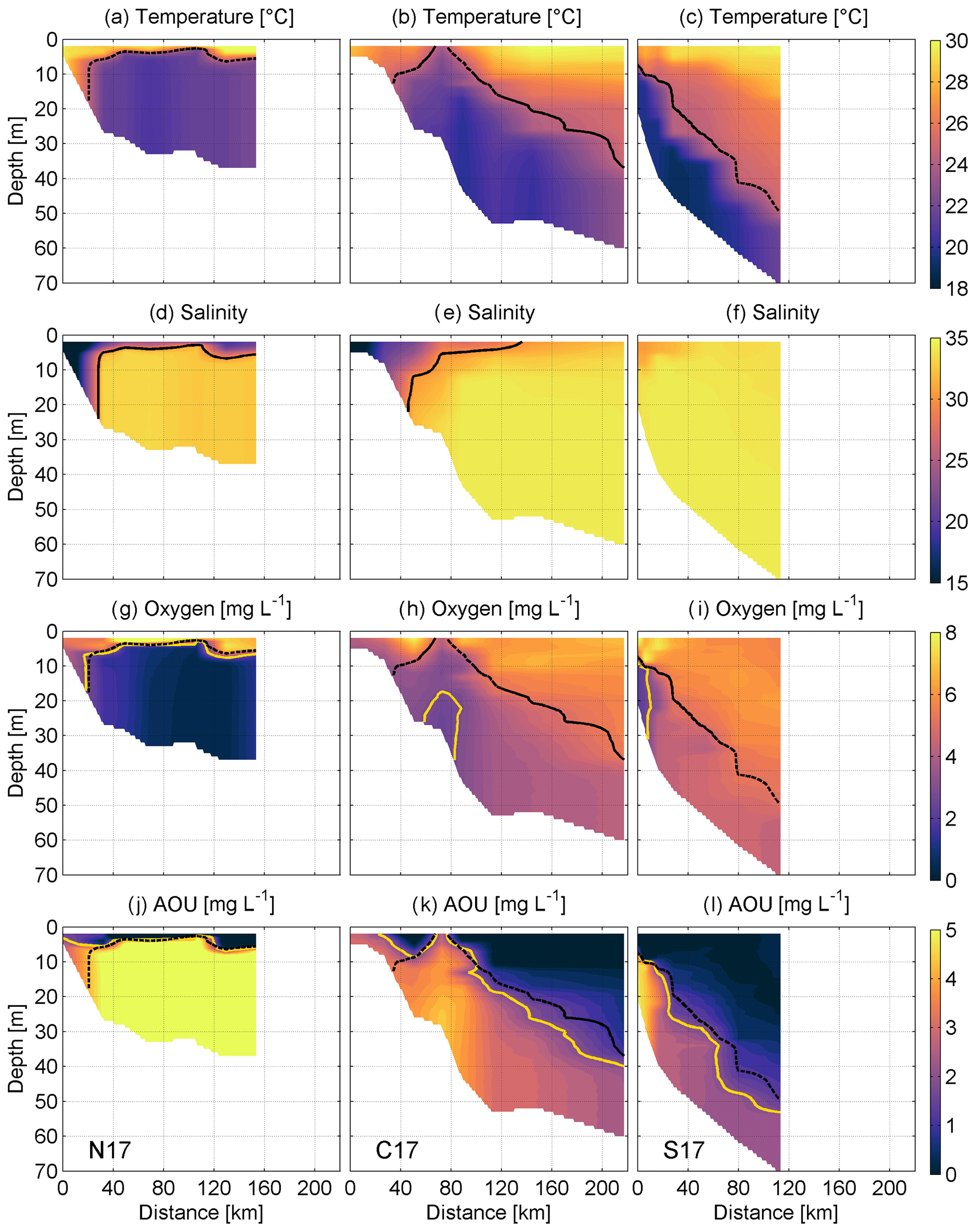
Figure 5Vertical distributions of temperature, salinity, density, DO concentration and AOU along sections N17, C17 and S17 in 2017 (Fig. 1). Temperature isoline 24.5 ∘C is shown with the dashed line in the temperature, oxygen and AOU plots. AOU isoline 2 mg L−1 is shown with a solid line in AOU plots. The hypoxia border (3.0 mg L−1) is shown with a solid line in oxygen plots. Locations of CTD stations are shown as crosses in the top panels. Values on the x axis indicate the distance from the westernmost point of a section (Fig. 1).
Spatial patterns of stratification in the study area are described by the density difference between the surface and near-bottom layer (Fig. 6a–b). Weaker stratification (< 3 kg m−3) was observed in the northern part of the study area in 2015 (Fig. 6a) when KSSW was present only at its offshore part (Fig. 4a). Stratification was stronger (> 3 kg m−3) in the area south of the Changjiang Estuary, being particularly strongest (>6 kg m−3) in areas of 20–30 m water depth (Fig. 6a), where the CDW covered the surface (Fig. 4e–f), and a cold and salty water mass occupied the bottom (Fig. 4b–c, e–f). From there, stratification declines rapidly onshore and offshore (Fig. 6a), because the dense, deep layer water could not intrude into the shallower areas (Fig. 4a–c) and the CDW could not spread further offshore (Fig. 3a, c, e, g). The upper boundary of KSSW had considerable inclination from 24 m depth near the coast to 48 m depth at 80–85 km offshore (indicating upwelling) in the southern section in 2015 (Figs. 4c, f and 7c). Opposite inclination (i.e., downwelling) was observed at the central station in 2015, with the boundary at 38 m depth near the coastal slope, tilting offshore towards 17 m depth (Fig. 4b, e). Downwelling had pushed the salinity 30 isoline down to 40 m depth along the central section in 2015 (Fig. 4e). It is probable that onshore transport of more saline offshore water over fresher coastal water caused vertical mixing.
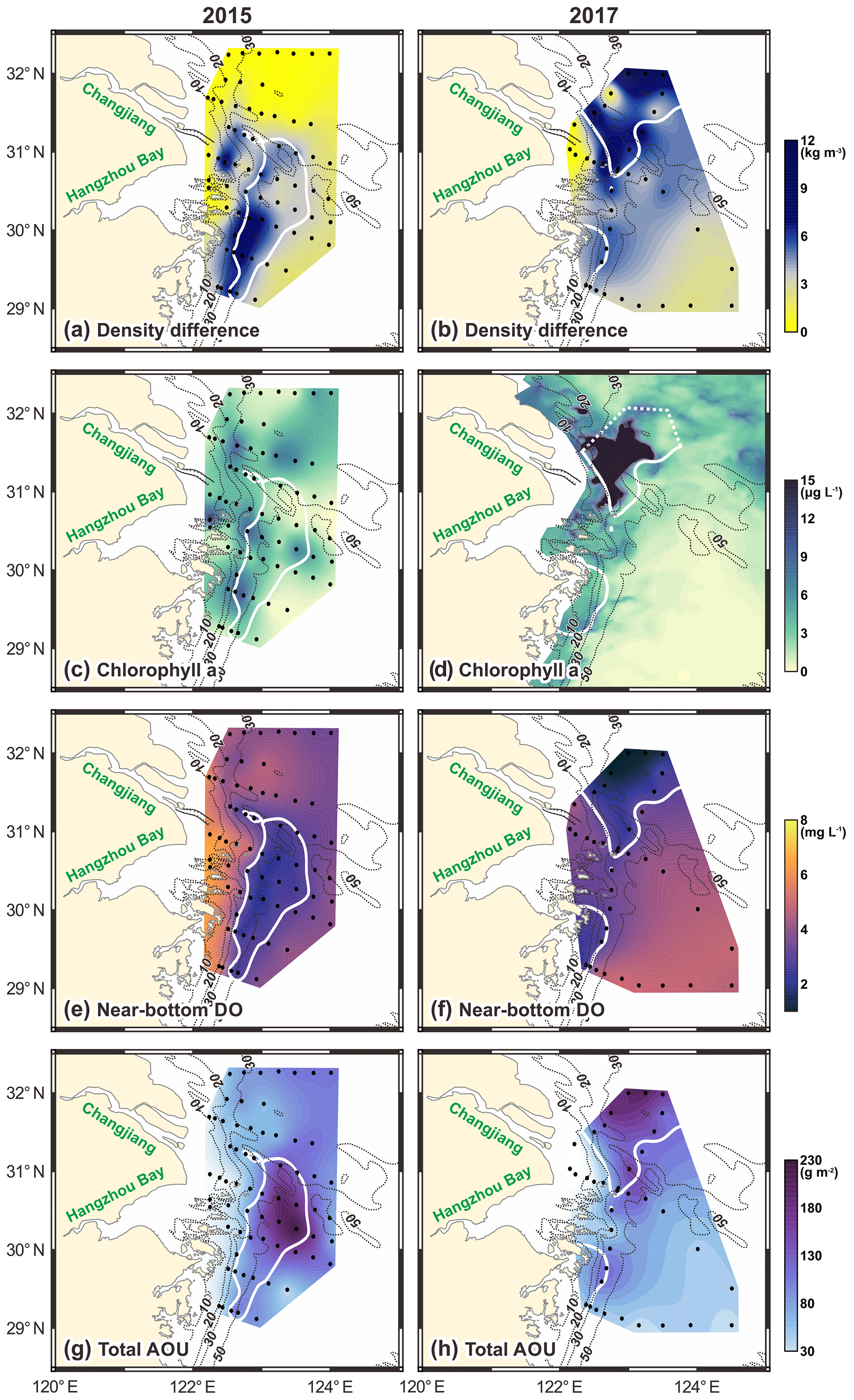
Figure 6Maps of density difference between the near-bottom layer and surface layer (a, b), in situ Chl a (c), satellite-derived Chl a (d), near-bottom DO (e, f) and total AOU in the water column (g, h). Maps of 2015 are shown on (a, c, e, g) and 2017 on (b, d, f, h). The remotely sensed Chl a map (f) is a mean field of two daily images of 21–22 July. AOU was calculated according to Eq. (3).
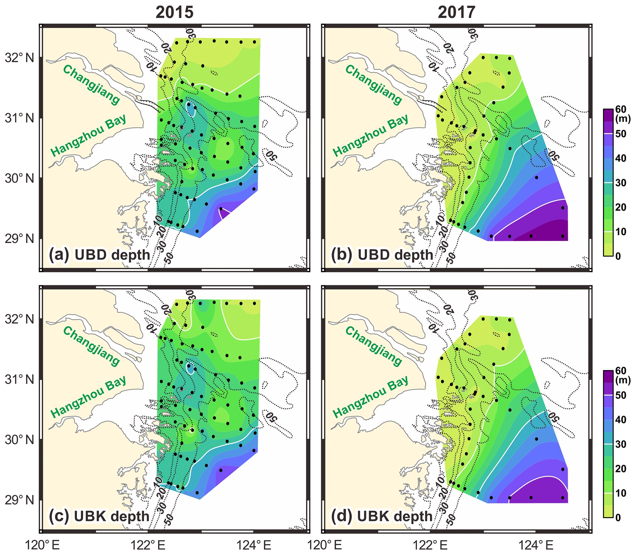
Figure 7Maps of AOU isoline 2 mg L−1 (upper boundary of the DO depletion) depth (a, b) and temperature isoline 24.5 ∘C (upper boundary of KSSW) depth (c, d) in 2015 (a, c) and in 2017 (b, d).
The strongest stratification (>6 kg m−3) was observed in 2017 in the northern part of the study area (Fig. 6b), where the cold upper boundary of KSSW was usually located at depths of 4–8 m (Figs. 5a, 7d). Above the strong pycnocline was warm and fresh CDW (Fig. 5a, d), whose extent coincided well with the very strongly stratified (>6 kg m−3) region (Fig. 3b). Stratification was weaker (<3 kg m−3) in the very shallow areas (<10 m, Fig. 6b), where the cold and saltier water mass did not exist, and in the southeastern part of the study area, which was influenced by the CDW but where bottom water was warmer than the core of the cold water mass (Figs. 3f, h and 5a–f). The stratification pattern in the central and southern section was characterized by the strong inclination of the isopycnals. The upper boundary of KSSW was located at 50 and 7–8 m depth at the eastern and western end of the 110 km long southern section, respectively (Fig. 5c, f). Surfaced upper boundary of KSSW (i.e., upwelling) was observed at 70–80 km distance in the central section (Fig. 5b). Warmer and fresher surface water was found both onshore and offshore from the upwelling core (Fig. 5b, e). Thus, the mixing of the riverine fresh water and upwelling water could be expected there.
Low DO concentrations (2–3 mg L−1) in the near-bottom layer occurred from 25 to 60 m water depth in the southern and central part of the study area in 2015, affecting an area of 1.3×10⁴ km2 approximately (Figs. 4h–i, 6e). Higher Chl a concentrations near the coast in the central and southern part illustrate the role of primary production in the CDW and subsequent processes resulting in oxygen consumption in the deeper layer (Fig. 6c). Although, due to downwelling, the low-DO water mass was pushed deeper and further offshore while the CDW was constrained closer to the coast (Fig. 4e h). Higher Chl a concentration at one station in the northern part (at 31.6∘ N and 122.6∘ E) coincided with the lower (<30) surface salinity intrusion (Fig. 6a). Elevated Chl a concentration further offshore (around 31.5∘ N and 123.2–123.5∘ E) did not coincide with the CDW (Figs. 3b, 6c). The upper boundary of the DO depletion and upper boundary of KSSW were strongly linked in the southern and central sections in 2015 (Figs. 4j–k, 7a, c). However, the boundaries coincided only on the offshore side of the northern section (Fig. 4j). That was the only section shown in Figs. 4–5, where the upper boundary of KSSW and the upper boundary of the DO depletion did not coincide (Fig. 4j). Likewise, this region differed from the rest (except shallower areas with water depth <20 m) of the observations by high near-bottom DO values (Figs. 4g, 6e). Near-bottom DO concentrations were 3–5 mg L−1 offshore the northern section but increased rapidly onshore in 2015 (Figs. 6e, 4g–i). The low-DO area (2–3 mg L−1) only overlapped partly with the CDW distribution but fitted well with the area occupied by the cold (<20 ∘C) water mass in the near-bottom layer (Fig. 4a–c, g–l). The vertically integrated AOU maximum (>150 g m2) pattern was observed between 30–31∘ N and 123–124∘ E in 2015 (Fig. 6g), which did not coincide with the Chl a distribution. In fact, very low Chl a concentration was observed at 30.5–31∘ N and 123–124∘ E (Fig. 6c) while oxygen depletion (total AOU) was rather high (Fig. 6e). We, therefore, hypothesized that oxygen depletion in the southern and central parts could have developed over longer periods.
Two low-DO-concentration zones were observed in the near-bottom layer in 2017 (Figs. 5g–i and 6f). The one in the north well overlapped with the low-salinity CDW and strong stratification area (Fig. 6b, f). Hypoxia there started at 4–8 m depth already and was closely linked to the location of the pycnocline (Fig. 5a, d, g). Thus, the thickness of the DO-depleted layer was 27–28 m in the northern part in 2017. The lowest DO and highest AOU of all our measurements were observed in the northern part in 2017 (Fig. 5g, j). Some profiles showed DO of nearly 0.6 mg L−1 and AOU over 6 mg L−1. High Chl a concentration was observed in the northern part, displaying the intense production in the upper layer (Fig. 6d). The second low-DO-concentration zone was found in shallow depths (10–30 m) at the coastal slope in the southern and central part of the study area and overlapped with lower SST and SSS upwelling region (Fig. 5b–c, e–f, h–i). This indicates that coupling between coastal upwelling, which bring subsurface water to shallower depths (euphotic zone), and CDW spreading created favorable conditions for the primary production in the upper layer and subsequent DO consumption and depletion in the deep layer (Fig. 5h, i, k, l). Higher Chl a concentrations in the upwelling area were revealed from the satellite image, although not as high as those in the north (Fig. 6d). The vertically integrated AOU had the highest values (>150 g m2) in the northern part of the study area in 2017 (Fig. 6h).
The high AOU zones in the near-bottom layer could be found at different water depths, e.g., as shallow as 4 m in 2017 (Figs. 4j–l, 5j–l). Strong and shallow stratification makes DO depletion possible in such a shallow depth. The question is whether the DO depletion is linked to a certain physical property of water, e.g., to temperature, salinity or density isoline. We found high correlation (r2=0.81, , n=44 in 2015, and r2=0.98, , n=34 in 2017) between the upper boundary of KSSW and the upper boundary of the DO depletion depth. Thus, the upper boundary of KSSW determines the vertical location of the upper boundary of the DO depletion largely. The cold KSSW is denser than the water above, and the resultant thermocline/pycnocline provides a barrier of vertical mixing to develop DO depletion below. There was an inclination of both isoclines in both years (Fig. 7). The inclination was particularly steep in 2017. Both isolines were located at >50 m depth in the southeastern corner of the study area, while in the shallow areas in the west and north the same isoclines were at 4–8 m depth (Fig. 7b, d). Such an inclination of isotherms and cold SST near the coast indicated upwelling. Deeper colder water intruded along the shallower coastal slope to replace the former upper layer water. The inclination of isoclines was not that pronounced and it was rather north–south directed in 2015 (Fig. 7a, c). Lower correlation in 2015 was caused by the discrepancy of the two isolines in the northern part in 2015. This indicates some processes other than KSSW intrusion, e.g., vertical mixing, vertical movement of pycnoclines or advection, altered subsurface conditions there.
It is noteworthy that the high vertically integrated AOU (Fig. 6g) area overlapped with a shallow position of isolines in 2015 (Figs. 4k, 7a, c,). The thickness of the DO-depleted layer in this area was 37–40 m in 2015. It means that high total AOU there (compared to neighboring areas) was related both to the thick subsurface DO-depleted layer and to the higher (compared to the surrounding area) AOU.
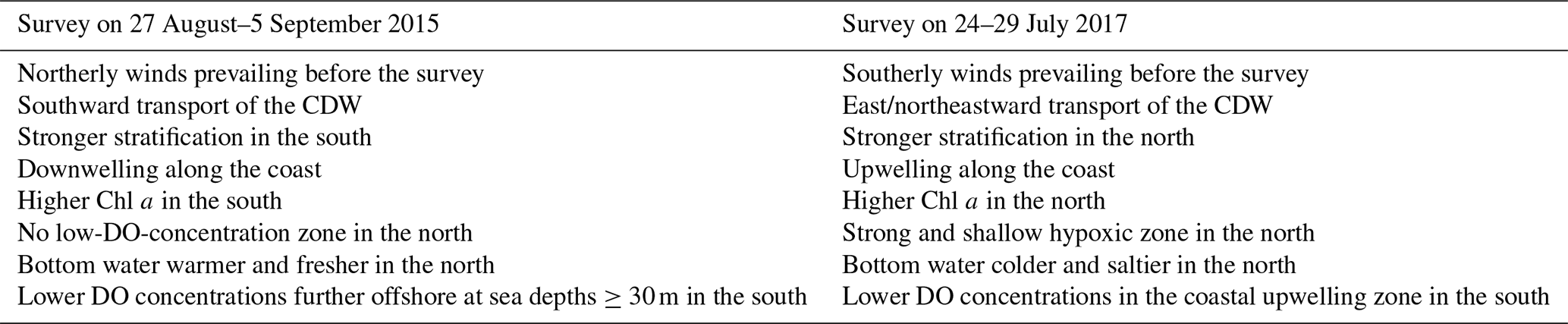
We have captured two completely distinct situations of stratification and DO distributions in summers 2015 and 2017. The differences between the two years are summarized in Table 1. Prevailing of either pattern in the physical fields should lead to varied biogeochemical fields and ecosystems in the area. The main questions addressed next are the following. What are the main drivers causing the distinct patterns? What is the forcing behind the formation of the patterns?
Table 1Summary of general features observed in the study area in summers 2015 and 2017.
3.2 Forcing behind distinct patterns in 2015 and 2017
The observed discrepancies of general features in the two cruise surveys can be driven by several forcing mechanisms. Two main factors can be considered to affect the distribution of CDW in the region: Changjiang River discharge and wind forcing. The riverine water is a source of buoyancy flux, causing the barotropic pressure gradient. The latter drives a current to flow south along the coast. Mean discharge at Datong hydrological station in the two summers (1 June to 31 August) was rather similar, 44 000–45 000 m3 s−1. We consider the time lag of 1 week for water propagation from Datong to the river mouth (Li and Chen, 2019) in further discussion.
In comparison, river discharge in June was higher in 2015, and in July it was higher in 2017. Daily discharge peaked at 58 000 m3 s−1 on 1 July 2015 and at 70 000 m3 s−1 on 13 July 2017. According to typical residual current velocities off the estuary (Peng et al., 2017) and along the coast in the south (Wu et al., 2013), it should take a few days to weeks for the water from the river mouth to reach offshore as registered in 2017 or to reach the southern part in 2015. We assume that 7 d of forcing (runoff or wind forcing) is enough to alter the field distributions off the estuary. Mean river flow in the week ahead of the surveys was 30 000 m3 s−1 in 2015 and 65 000 m3 s−1 in 2017. Variations in discharge influence the cross-shore extent of plume and the width of the buoyant current. According to Eq. (4), the width Wp of the buoyant current would be 77 km in the case of an ambient and CDW water density difference of 10 kg m−3, a coastal slope of 10−4, and a discharge of 65 000 m3 s−1 before our survey in 2017. The width would be 55 km for the inflow volume of 30 000 m3 s−1 in 2015. Thus, the variability in the river discharge only partly explains the discrepancy between the two surveys, particularly more extensive spreading of the CDW eastward in 2017. However, it does not explain the northeast advection of the CDW that far in 2017. Likewise, it remains unclear why southward transport of the CDW was much more limited in 2017 than 2015. Several indicators hint that wind-driven transport could have caused the differences between the 2015 and 2017 observations, including stronger cross-shore inclination of the pycnocline (Fig. 7d), offshore advection of the CDW and onshore advection of the colder subpycnocline water in 2017. Such features were not found during the survey in 2015, but southward advection of the CDW was revealed instead. Since our surveys are conducted annually 1 month apart, the differences between the two surveys might be associated with the annual cycle in wind forcing. Our hypothesis is that the dominant factor behind the discrepancy of the two surveys is wind forcing and possibly its seasonality.
As described previously, we assume the thermohaline fields in the study area were established by the forcing 1 week before the sampling. Mean wind, sea level anomaly, surface currents and bottom currents during 7 d before the surveys are presented in Fig. 8. The mean wind direction was from the northeast before the 2015 survey (Fig. 8a) and from the south before the 2017 survey (Fig. 8b). Northeasterly wind should cause downwelling and accelerate alongshore buoyant current toward the south. This current was visible in the mean surface current plot in 2015 (Fig. 8c), along the coast from 32.5 to 28∘ N. Such a coastal current did not prevail before the 2017 survey (Fig. 8d). Weak mean flow towards the east or northeast could be noted near the mouth of the Changjiang River in 2017 (Fig. 8d). The buoyant coastal current was probably altered, and the CDW was transported across shore by southerly wind forcing. Thus, simulated current patterns and wind forcing before the two surveys were qualitatively in accordance with observed salinity fields in the surface layer (Fig. 3a–b). The main difference between the two years in the bottom layer was the stronger northward flow in 2017 (Fig. 8e–f). The penetration of the deep layer water to the shallower areas, towards the river mouth, occurred in 2017 (Fig. 8f). This coincided with our observations in terms of the stronger inclination of clines (Fig. 7b, d) and presence of the colder KSSW water mass in the northern part of the study area in 2017 (Fig. 3h). Because southerly wind caused offshore transport of the surface water, deep layer water intruded to the shallower depths for compensation in 2017. The observed patterns based on field surveys and modeling data can be confirmed by the mean sea level anomaly during the surveys (Fig. 8g, h). There is a strong sea level gradient between nearshore and offshore in both years. Higher sea level can be found along the coast from the northern boundary of the study area to 30∘ N in the south in 2015, and as a result, the geostrophic current is southward. This is the combined effect of the lighter riverine water and convergence of the shoreward-transported upper layer water. This is in accordance with our observation of the downwelling in the central section (Fig. 4b, e, h, k), while such a phenomenon did not occur in the southern section (Fig. 4c, f, i, l) in 2015. Downwelling co-occurred with the alongshore southward current in the northern part according to the sea level anomaly (Fig. 8g) and simulated current field (Fig. 8c). This could explain the well-ventilated and warmer near-bottom waters in the north in 2015 (Fig. 4a, g, j). An opposite gradient, i.e., lower sea level anomaly near the coastline, was observed in 2017. This is a typical sign of divergence, i.e., offshore transport of the surface water and consequent upwelling along the coastline. The zonal pattern of sea level from the river mouth to offshore (high–low–high sea level, Fig. 8h) agrees with our observation of the upwelling in the central section (Fig. 5b, e). As a result of sea level anomalies, geostrophic currents toward the north at 28.5–31∘ N and offshore near the river mouth were observed in 2017.
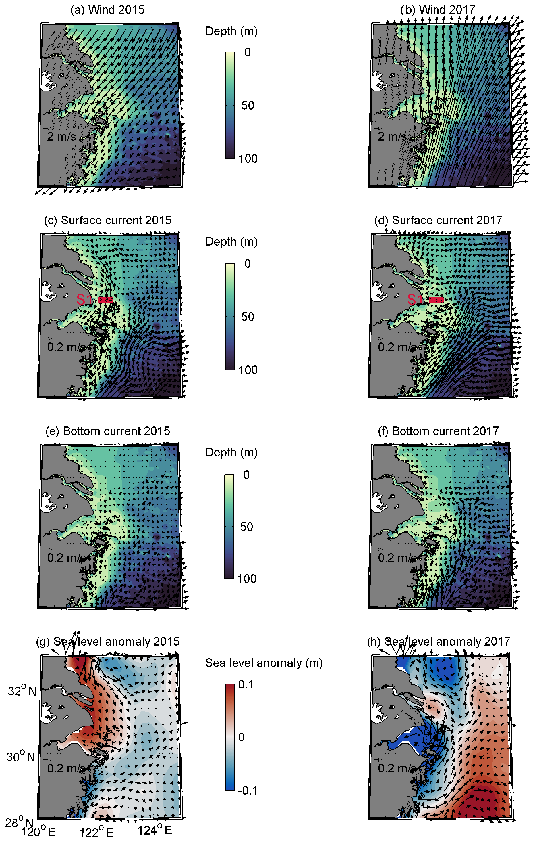
Figure 8Maps of mean wind (a–b, m s−1), simulated surface current (c–d, cm s−1) and bottom current (e–f, cm s−1) in the sea bottom depths down to 100 m during the 7 d period before the CTD surveys. Bottom bathymetry is shown as a background in (a)–(f). Red lines in (c) and (d) show section S1, where current time series (presented in Fig. 10c) were calculated. Every fourth current vector is shown only in (c)–(f). Mean sea level anomaly (m) as contours and geostrophic velocities (cm s−1) as vectors derived from satellite altimetry during the surveys are shown in (g)–(h).
3.3 Variability and drivers of the Changjiang Diluted Water spreading
In order to verify the sensitivity of the buoyant coastal current to wind forcing, simulated current and wind data from June to September in 1993–2018 were used. First, we calculated the daily mean meridional (alongshore) upper layer (0–5 m) current velocity component vm at the zonal section of 31∘ N (section S1) from 122.1 to 122.6∘ E (see red line in Fig. 8c–d). Secondly, the correlation was calculated between the current velocity component vm and wind (see the location in Fig. 1) from different directions (full circle by 10∘ steps) and by different time lags shifted by 1 d step. The best correlation (r2=0.76, , n=3025) was found with the 1 d (prior to the modeled current value) mean SE–NW wind velocity component wc (Fig. 9). Thus, the meridional current along the coast correlates well with wind.
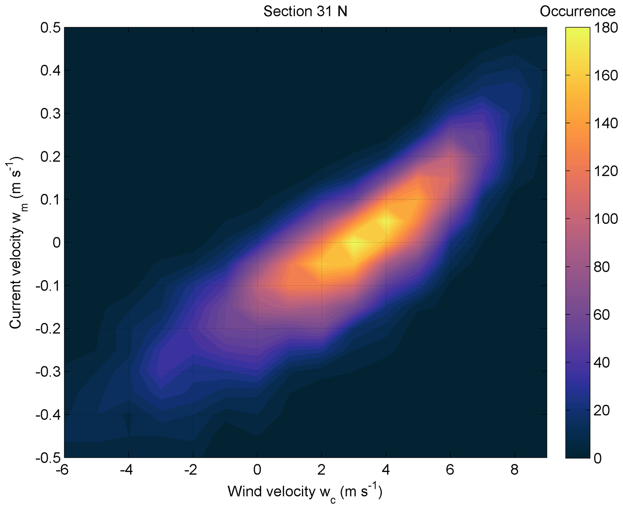
Figure 9Relation of daily mean SE–NW wind velocity component wc (positive towards NW) and meridional current velocity component vm (positive northward) in the section at section S1 (see Fig. 8) in 1993–2018. The color scale shows the co-occurrence (number of cases) of respective wind velocity and current velocity component combinations.
Simulated near-bottom currents (Fig. 8f) suggest that colder and saltier water (compared to 2015 observation) was advected to the northern part of the study area as compensation flow to the near-surface offshore flow in 2017. Moderate winds before the 2017 survey (Fig. 10a) could not mix the cold and DO-depleted deep layer water into the upper layer. However, stronger wind impulse with speeds up to 11–12 m s−1 occurred a few days before the start of the survey in 2015 (Fig. 10a). Upper mixed layer depth created by wind stirring was estimated by the formula describing the turbulent Ekman boundary layer (Csanady, 1981), where is friction velocity, ρw is water density, τ is wind stress, and f is the Coriolis parameter. Vertical mixing reached down to 15–16 m depth according to this empirical method before the 2015 survey. Note that our estimation is based on 6 h average wind speed. Stronger winds, which occur on shorter timescales, probably cause deeper mixing. Thus, wind stirring could weaken the stratification before the 2015 survey, as evidenced by the presence of warmer, fresher water with higher DO concentration in the deep layer. However, advection from the north (Fig. 8c) and downwelling (Fig. 8g) likely also contributed to the weakening of stratification and ventilation of the northern part in 2015. Water from the north is colder and causes convective mixing and weakening of the thermocline. The effect of downwelling can be seen in the central section (Fig. 4b, e, h, k). Seafloor is flatter in the northern part and therefore the subthermocline distributions in the case of downwelling showed up there as lateral gradients (Fig. 4a, d, g, j).
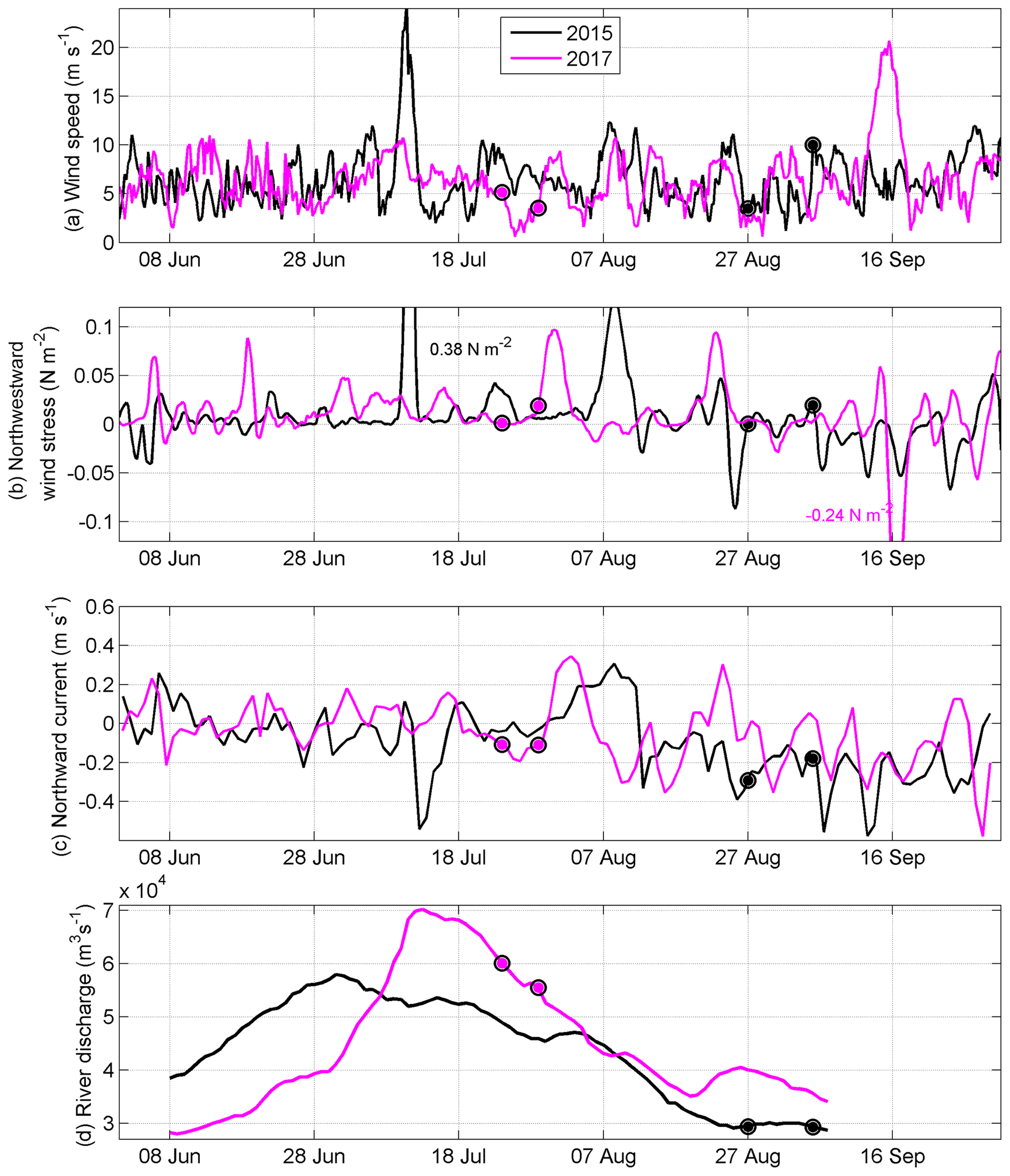
Figure 10Time series of wind, current and river discharge. Mean wind speed (6 h) (a), 1 d running mean SE–NW wind stress τc (positive towards NW; N m−2) (b), daily mean meridional current velocity component vm (positive northward) at section S1 (c), and daily Changjiang River discharge at Datong station shifted by 7 d to represent flow in the river mouth (d). Dots represent the start and end of the CTD surveys, respectively in 2015 and 2017.
We further analyzed time series of wind speed (Fig. 10a), the SE–NW wind stress component (τc, Fig. 10b), the meridional current velocity component (vm, Fig. 10c) at section S1, and the Changjiang River runoff (Fig. 10d) in June–September 2015 and 2017. Wind stress τc>0 and a northward current component prevailed from June to early August in 2017 (Fig. 10b). Larger wind stress events alternated with calmer periods from June to late August in 2015. During the periods of τc<0 or weak northward winds, the current was often directed southward. The vm<0 occurred more frequently in June–July 2015 compared to the same period in 2017 (Fig. 10c). The latter is reflected in salinity distributions (Fig. 3a–b). We defined the CDW as salinity <30 and calculated its monthly spatial occurrence from June to September in 2015–2018 using satellite surface salinity distributions (Fig. 11). The lowest areal extent of the CDW was observed in September in both 2015 and 2017. The CDW was mainly transported to the northeast and east in all summer months in 2017. Northeastward transport of the CDW could also be noted in 2015, but the CDW occupied areas in the southern part of the study area as well. Thus, the satellite-derived salinity confirms our in situ observations of the southward flow of the CDW. We can conclude that our survey in 2017 describes the prevailing situation of the CDW spreading in summer 2017 well. In 2015, we captured the situation where the CDW spread to the south, but during summer, northeastward spreading occurred as well (Fig. 11). The CDW spreading in 2016 and 2018 was rather northeastward (similar to 2017). The CDW spreading presented in Fig. 11 is further analyzed in relation to interannual wind and river forcing, as well as in the context of previous studies in the discussion.

Figure 11Maps of monthly occurrence (%) of (remotely sensed) salinity <30 from June to September in 2015–2018.
Next, we attempt to link the CDW spreading, i.e., coastal current velocities, to the wind forcing in the period June–September in 1993–2018. We grouped the simulated meridional currents vm at section S1 (see Fig. 8c–d) to the wind velocity wc classes with the step of 0.25 m s−1 and took an average of each group. By doing this, we found a relation between mean wc and vm. If the daily mean wind velocity component wc=0 m s−1, the current velocity component vm would be on average −13 cm s−1 (i.e., southward) at S1. We can assume that this is the mean geostrophic component of the current velocity. A daily mean wind velocity component wc of 5.6 m s−1 is required to reverse the current and have the same magnitude at S1 ( cm s−1). This corresponds roughly to the wind stress τc of 0.04 N m−2. Wind stress τc of 0.02 N m−2 corresponds to vm=0 cm s−1; i.e., coastal current is altered. We define vm=0 cm s−1 as the term “alteration of the coastal current” in the rest of this paper. Two main wind-driven processes contribute to the alteration of the coastal current. First is the direct effect of wind stress and the resulting Ekman surface current. Secondly, southerly winds cause divergence and upwelling at the coast and alter sea level distributions. When upwelling is evoked, the alongshore geostrophic current, resulting from the cross-shore gradient between colder–denser and warmer–lighter offshore water, is rather to the north. The mean sea level anomalies during our surveys in 2015 and 2017 illustrate this phenomenon well (Fig. 8g–h). The joint effect of the two processes explains why relatively low wind stress is required for the alteration of the circulation regime. We analyzed the simulated current data in June–September from 1993 to 2018 and averaged the cases when the daily mean wind stress component τc was <0 and ≥0.02 N m−2 (Fig. 12). The same circulation features, but more pronounced, stand out as before the surveys in 2015 and 2017 (Fig. 8). In the case of τc≥0.02 N m−2 surface flow was northward along the coast and to the northeast near the river mouth (Fig. 12a), while it shifted north or towards the river mouth in the deep layer (Fig. 12c) as before our survey in 2017 (Fig. 8d, f). In the case of τc<0 N m−2 southerly flow prevailed in the surface layer along the coast (Fig. 12b), and the mean currents in the near-bottom layer were rather weak (Fig. 12d) as before our survey in 2015 (Fig. 8c, e). This supports our hypothesis that the wind field is a key forcing driver for the direction of the Chinese Coastal Current controlling the CDW distribution off the Changjiang Estuary and thus hypoxia formation (Fig. 8a–f).
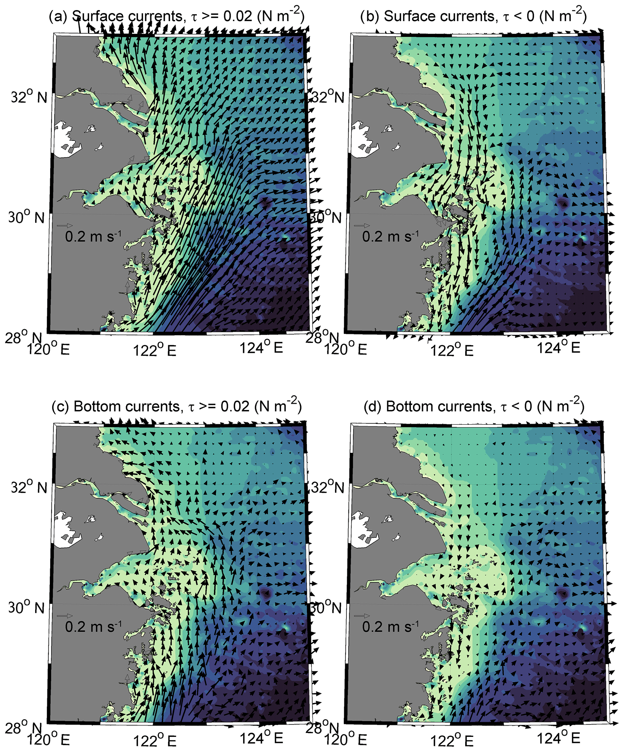
Figure 12Maps of surface (a, b) and near-bottom (c, d) currents in the sea bottom depths down to 100 m in the cases of wind stress component τc≥0.02 N m−2 (a, c) and τc<0 N m−2 (b, d) in 1993–2018. Every fourth current vector is shown.
The balance between oxygen consumption caused by the decomposition of organic matter by bacteria in the subsurface layer and oxygen supply controls the formation of hypoxia in the ECS. There is a strong link between primary production in the upper layer and oxygen consumption in the near-bottom layer (Chen et al., 2017, 2004; Wang et al., 2017, 2016; Wei et al., 2017a; Zhou et al., 2019). The processes accompanied by enhanced primary production, the spreading of the riverine nutrient-rich CDW and KSSW upwelling, are dependent on wind and river forcing. Likewise, physical processes, which can supply the deep layer with oxygen, lateral advection and vertical mixing, are partially driven by wind forcing.
Two distinct stratification, Chl a and DO distribution patterns were observed in the area off the Changjiang Estuary in the summers of 2015 and 2017. There was a stronger DO depletion in the southern part of the study area in August–September 2015 (Fig. 6e), while intense hypoxia was observed in the northern part of the study area in July 2017 (Fig. 6f). Likewise, remarkable DO depletion was found in the southern part in the upwelling region in 2017 (Fig. 6f). Similar hypoxia patterns in August (as we observed in July 2017) and October (as we observed in August–September 2015) were observed in 2006 (Zhu et al., 2011). The main reasons for the different spatial hypoxia patterns are variations in the wind forcing and river discharge. Southeasterly winds and higher discharge during the summer monsoon both favor cross-shore transport of CDW and development of hypoxia in the northern part of the study area. Both the maximum frequency of southerly wind and river discharge in the annual cycle occurred in July–August (Fig. 13a, c). In accordance with the annual cycle of wind (Fig. 13a), the highest frequency of upwelling events occurs in July–August as well (Xu et al., 2017). Thus, our observations conducted in late August/early September 2015 and late July 2017 illustrate the seasonal cycle of forcing and are reflected in DO and stratification patterns. The summer monsoon and river discharge were close to average in the whole summer of 2017, while the summer monsoon was weaker in 2015 (Fig. 13a–b). Wang et al. (2012) explained the annual cycle of the location of near-bottom DO minimum by the seasonal change in regional stratification and variations of the northward extension of the KSSW. An idealized numerical experiment has shown that northerly winds reduce hypoxic area while westerly winds expand it (Zheng et al., 2016).
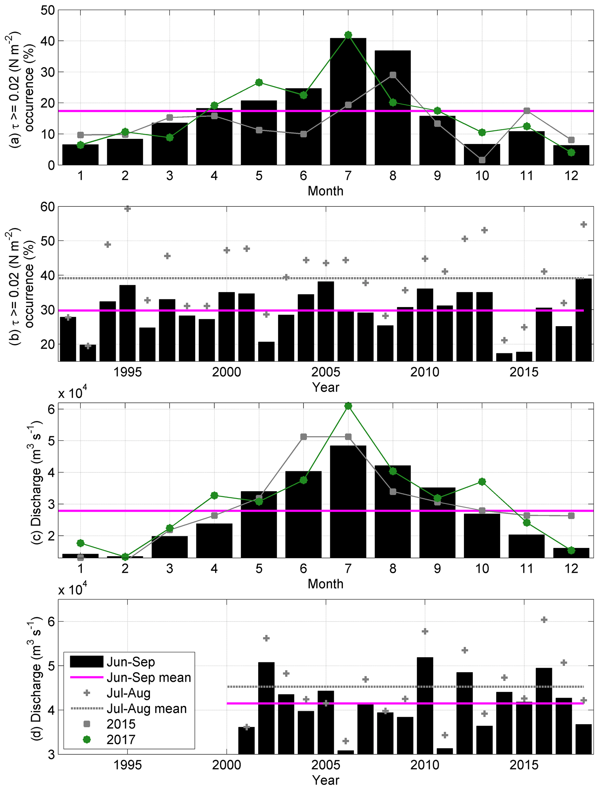
Figure 13Annual cycle (a, c) and interannual variability (b, d) of wind stress component (1992–2018) τc≥0.02 N m−2 (a, b) and river discharge (c, d) (2001–2018).
The monthly occurrence of CDW clearly shows that CDW transport offshore (to northeast) prevailed during summer periods (Fig. 11). However, one can see that 2015 differed with low values in the interannual time series of wind stress of τc≥0.02 N m−2 (Fig. 13a–b) and with considerable southward advection of the CDW (Fig. 11). Monthly maps of bottom oxygen in 2015 (Z. Li et al., 2018) do not show significant oxygen depletion in the north in any month, while deteriorated hypoxia (compared to our observations) occurred in the south in October (Z. Li et al., 2018). This well demonstrates that the wind regime plays an important role in the interannual variations of the hypoxic area location (Fig. 6e–f). The year 2016 stands out in terms of very high river discharge (Fig. 13d) and wind forcing close to the interannual mean (Fig. 13b). One can see that offshore advection prevailed in 2016 (Fig. 11). Thus, it indicates that if wind forcing is close to the long-term average, then hypoxia will more likely occur east of the river mouth (northern part of the study area) and hypoxia occurrence in the south will be more limited. That was confirmed by our observations in 2017. River discharge and wind stress τc≥0.02 N m−2 were both similar to the long-term mean in 2017 (Fig. 13), and we observed hypoxia and CDW water in the northern part. It means hypoxia in the southern part (as we found in 2015) occurs if the summer monsoon is considerably weaker than the long-term mean. Indeed, hypoxia in the south was quite rare in 1998–2013 (Chen et al., 2017). As a consequence of large river runoff, the largest CDW extent occurred in the year 2016 out of the 4 years (Fig. 11). The occurrence of wind stress τc≥0.02 N m−2 was higher than average (Fig. 13b) and river discharge was lower than average in 2018 (Fig. 13d), and this reflected well in the CDW (Fig. 11). One can see that CDW covered the smallest area out of 4 years, and the prevailing transport direction was towards the north or northeast (Fig. 11). From our stratification and DO distribution observations (Figs. 3–7) and their dependence on wind forcing (Figs. 8–10, 12), as well as CDW spreading direction and extent (Fig. 11), DO-depleted area could have occurred in the northern part both in 2016 and 2018, with the larger extent in the former year. The positive correlation between the river discharge and the hypoxic area has been found by the model simulation (Zheng et al., 2016). Hypoxia in the northern part in 2016 was reported (Zhang et al., 2019). Lower-than-average river discharge and close-to-average wind stress of τc≥0.02 N m−2 (as in 2016) occurred in 2006 (Fig. 13b, d) when hypoxia was registered in the north (Zhu et al., 2011).
We estimated that wind stress of τc≥0.02 N m−2 is necessary to alter the geostrophic coastal current and create favorable conditions for hypoxia in the northern part. Following higher interannual occurrences of wind stress τc≥0.02 N m−2 in July–August (Fig. 13a), the larger hypoxic area in the north was documented for instance in August 2012 (Li, 2015) and August 2013 (Ye et al., 2016; Zhu et al., 2017). In contrast, in summers when the occurrence of τc≥0.02 N m−2 was lower, considerable DO depletion was also expected to have occurred in the southern part, as observed, e.g., in 1998 (Wang and Wang, 2007) and 1999 (Li et al., 2002). However, on top of the interannual variability and seasonality, synoptic-scale changes in wind-driven currents and river forcing are likely to influence the distributions on shorter timescales (Fig. 10). Thus, when planning measurement campaigns, it is worthwhile to take into account wind-driven transport, river discharge, remotely sensed salinity and altimetry to forecast spreading of the CDW, as well as upwelling occurrence and deep water intrusion. That allows us to estimate potential hypoxic area and therefore more efficient use of ship time and more detailed sampling of the hypoxic area.
The fate of the river plume can be separated into two regions and processes: the circulating bulge near the river mouth and the downstream coastal current (Fong and Geyer, 2002; Horner-Devine, 2009). It has been estimated that about 80 %–90 % of the river discharge is transported alongshore with the coastal current (Li and Rong, 2012; Wu et al., 2013). That means that most of the river discharge does not remain in the river plume bulge but impacts the surrounding areas off the estuary. We estimated the southward geostrophic component of the current velocity to be on average 13 cm s−1 at section S1. The southward coastal current was measured in winter by Wu et al. (2013). They estimated the maximum current speed up to 50 cm s−1, including also the wind-driven component, which supports flow to the south in winter (Wu et al., 2013).
Offshore, east- or northeastward-advected CDW caused by southerly wind, as we observed in 2017, might form detached eddies due to interaction of the Ekman flow and density-driven frontal currents (Xuan et al., 2012). Those eddies bring CDW further offshore and alter physical and chemical characteristics (including DO conditions) and primary production in the water column (Wei et al., 2017b).
Offshore-transported CDW co-occurred with coastal upwelling caused by southerly wind in 2017. Shoreward, upslope penetration of the subthermocline KSSW and hypoxia in the upwelling–CDW interaction zone (Wei et al., 2017a) were observed. Upwelling, induced by southerly winds and its relaxation supported by northerly winds, was also found by Yang et al. (2019). Wei et al. (2017a) showed that the coupling of the CDW plume front and KSSW upwelling caused DO minimum at the sloping bottom. Likewise, the nitrogen-to-phosphorus ratio and primary production in the CDW are considerably modified by upwelling (Tseng et al., 2014). Phosphate transport by upwelling reduces phosphorus deficiency in the CDW water and, therefore, promotes phytoplankton growth and nitrate uptake (Chen et al., 2004; Zhou et al., 2019).
Time series of wind displayed large variations in wind forcing on shorter timescales (days to weeks) (Fig. 10) which may alter the stratification pattern and DO distributions considerably. Numerical simulation by Zhang et al. (2018) showed that wind-induced redistribution of the Changjiang River plume changes near-bottom DO conditions rapidly. Also, it has been shown that vertical mixing caused considerable variations in DO concentrations in the near-bottom layer (Ni et al., 2016). Higher wind speed causes stronger vertical mixing and vanishing of hypoxia (Zheng et al., 2016). In July 2015, 1.5 months before our survey, hypoxia was terminated by a typhoon, but 2 d later, hypoxic conditions were reestablished (Guo et al., 2019). Our field measurements showed that the upper boundary of the DO depletion is strongly linked to the upper boundary of KSSW (Fig. 7). Besides enhanced (or impeded) vertical diapycnal mixing, DO conditions can be altered by vertical movement of this water mass. Ni et al. (2016) published a valuable time series of DO in the near-bottom layer. They linked the increase in DO concentrations in the near-bottom layer with the vertical mixing and the DO decline in the near-bottom layer with the primary production and consequent decomposition of detritus. One can see several cases from their time series data (Fig. 2 in Ni et al., 2016) when the near-bottom temperature drops. Those events must be related to the advection of colder water and uplift of the KSSW as DO declined during those events. Penetration of the cold, low-DO water upwards along the coastal slope appears when temperature and DO decline in the point measurement time series. There are some registered events when the near-bottom layer temperature rises, but sea surface temperature does not change much (e.g., Fig. 2 in Ni et al., 2016). In these cases, DO concentrations increased in the near-bottom layer. Such events can be associated with the downward movement of the thermocline or advection of warmer water, as we observed in the central section in 2015 (Fig. 4b, e, h, k) rather than vertical mixing. Thus, vertical location and movement of the thermocline have an important role in the near-bottom DO distributions at the coastal slope. The importance of KSSW thickness on the oxygen depletion is also revealed when near-bottom DO maps are compared with the maps of vertically integrated AOU (Fig. 6g–h). Bottom hypoxia in the north in 2017 was much more intense compared to hypoxia in the south in 2015. However, the total AOU was similar in hypoxic zones in both years due to the thicker DO-depleted layer, i.e., thicker KSSW in the south in 2015.
Studies of pycnocline dynamics, including downwelling studies, as suggested by Hu and Wang (2016), are essential in future investigations. Those studies are difficult to arrange with conventional research vessel surveys only. Autonomous measurement platforms, such as profiling moorings (Lips et al., 2016; Sun et al., 2016) and moored sensor chains (Bailey et al., 2019; Venkatesan et al., 2016), which allow capturing the variability in the necessary spatiotemporal resolution, can be used. Underwater gliders (Liblik et al., 2016; Rudnick, 2016) might be complicated to use due to strong tidal velocities and heavy ship traffic but are worth considering as well. Despite strong tidal oscillations, the vertical average of residual current speeds in the area (Peng et al., 2017) is smaller than the forward speed of gliders. Moreover, adaptive piloting methods can be used to control a glider (Chang et al., 2015).
Our observations indicated that two conditions in the water column must be present for the development of hypoxia. First, high AOU occurred only below the thermocline, in the cold KSSW. Secondly, primary production in the fresher CDW or upwelling is needed to cause high DO consumption that leads to hypoxia. Interestingly, these two conditions for hypoxia formation were valid in very different situations. The shallow (4–6 m depth) and sharp thermocline coincided with the halocline (related to the CDW) in the northern part of the study area in 2017. In contrast, the thermocline and halocline were separated in the southern part of the study area in 2015. Thus, the vertical coincidence of halocline and thermocline is not necessary for the hypoxia formation. The thermocline acts as a physical barrier, which impedes vertical mixing and DO exchange with the upper layer. Primary production in the CDW or the upwelled water and related DO consumption in the near-bottom layer (Wang et al., 2017, 2016) causes DO decline. Zhu et al. (2016) found that the area of DO concentration <3.0 mg L−1 fits relatively well with the region of the pycnocline strength >2.0 kg m−3. This relationship between pycnocline strength and low DO only partly holds according to our analysis (Fig. 6a–b, e–f). For instance, there was strong stratification (Fig. 6a) near the river mouth (around 122.5∘ E and 31∘ N) in 2015 due to the presence of the CDW, but hypoxia was not observed (Fig. 6e) since the colder KSSW was not present. Most of the study area, except very shallow areas, had strong enough stratification (pycnocline strength >2.0 kg m−3) in 2017 (Fig. 6b). However, hypoxia in the southern part in 2017 was only observed near the coast and in connection to the coastal upwelling (Fig. 6f). The rest of the study area in the south was free of hypoxia. In the latter area, KSSW was present but there was no CDW in the surface layer. That means that strong stratification as such does not necessarily lead to hypoxia. Two features must be present for hypoxia formation: (1) KSSW and (2) CDW and/or subsurface water upwelling. We can conclude that colder KSSW determines where (including at what depths) hypoxia could develop; i.e., it provides the necessary precondition for hypoxia. The CDW spreading and/or subsurface water upwelling (and related biogeochemical and biological processes) determine the magnitude, exact location and timing of oxygen depletion. Both features are strongly impacted by wind.
Besides the barrier effect of the thermocline, the intrusion of KSSW has another impact on oxygen dynamics. The subsurface water is DO-depleted already before the local impact of DO consumption (Qian et al., 2017). The stations in the farthest southeast (Fig. 1) had AOU of 2–2.5 mg L−1 in the deep layer in 2017, i.e., in the same order that has been estimated in the KSSW before (Qian et al., 2017). The total AOU in the water column there was 50–60 g m−2 (Fig. 6h). This water was still rather well ventilated compared to the deep layer waters that had been impacted by upwelling or CDW-induced production in the surface layer (Fig. 6g–h). Despite its initial DO depletion, Kuroshio intrusion is an important source of oxygen import to the study area (Zuo et al., 2019). Without this lateral DO transport, hypoxia could form much faster in a larger area (Zuo et al., 2019). Kuroshio intrusion is nutrient-rich (L. Zhang et al., 2007; Zhou et al., 2019) and its upwelling or vertical mixing could intensify primary production in the surface layer; consequently organic matter sinking causes DO consumption in the near-bottom layer.
We have already outlined the main difference in the wind forcing, causing the formation of hypoxia in the southern and northern parts of our study area. The one in the north develops under the conditions of the summer monsoon. Intensive hypoxia can start from very shallow depths (at 4–8 m) in the northern area (Fig. 5g), and it can develop very fast under favorable conditions (Guo et al., 2019). At the same time, the bottom layer there can be easily ventilated by wind stirring or downwelling as we observed at section N15 in 2015 (Fig. 4g). Thus, hypoxia in the northern part can be very pronounced but also may disappear fast if forcing changes (Ni et al., 2016).
Hypoxia in the southern part of the study area was not as pronounced but quite stable as noted already by Zhu et al. (2011). The decline of the DO from March to October in the southern part was demonstrated by monthly measurements (Z. Li et al., 2018). We suggest three main reasons for this. First, favorable wind conditions for the southward transport are not that frequent in summer. Second, the mixture of CDW with ambient ocean water promotes primary production and subsequent settling of organic matter on its way south. So less detritus sinks to the bottom layer, and DO consumption is lower in the southern part compared to the northern region. Third, the KSSW and related thermocline are located deeper in the south, and therefore wind mixing does not diminish the thermocline. The first two reasons account for weaker hypoxia and the third for long-lasting hypoxia in the southern part.
Two main conditions in the water column must be present for the occurrence of hypoxia in the near-bottom layer off the Changjiang Estuary: enhanced primary production in the upper layer and KSSW intrusion in the near-bottom layer. Pycnocline created by KSSW intrusion or CDW spreading is the precondition and determines where hypoxia could develop. Primary production in the CDW and/or in the upwelled water and consequent oxygen consumption by sinking organic matter below the pycnocline determine the magnitude, exact location and timing of oxygen depletion. Both the distribution of CDW and KSSW and the occurrence of KSSW upwelling are controlled by the wind field.
The summer monsoon (wind from south) alters the Chinese Coastal Current by creating an Ekman surface flow and by changing the geostrophic current flowing to north or northeast. As a result, the CDW spreads offshore, and KSSW intrudes northwards and upwards on the coastal slope, resulting in upwelling. The joint effect of these processes can lead to intense and shallow (4–8 m) oxygen depletion in the north and hypoxia at the coastal slope in the south.
Northerly wind intensifies the Chinese Coastal Current and CDW spreading to south, and it causes downwelling. Consequently, the northern part is well ventilated and hypoxia rather occurs further offshore in the southern part.
Wind forcing and river runoff are important contributions to interannual and seasonal variations, determining the size and location of low-DO areas. The DO minimum is located more likely in the northern part in July–August and the southern part during the rest of the stratified period.
If wind forcing is close to the long-term average during summer, hypoxia more likely occurs in the northern part of the study area. If the summer monsoon is considerably weaker than the climatic average, hypoxia rather occurs in the south. Thus, interannual variations in the location of the hypoxic area are largely controlled by wind forcing.
There is a strong connection between the upper boundaries of KSSW intrusion and oxygen depletion. The sensitivity of the boundaries to wind forcing shapes oxygen conditions in the area considerably. Autonomous measurement campaigns by mooring arrays and underwater gliders could considerably improve the knowledge about related processes. Our results further suggest that a combination of wind field data, river discharge, remotely sensed sea surface salinity and sea level could be used to forecast the hydrographic conditions and potential hypoxic area before field work.
Scripts to analyze the results are available upon request. Please contact Taavi Liblik (taavi.liblik@taltech.ee).
The supplement related to this article is available online at: https://doi.org/10.5194/bg-17-2875-2020-supplement.
TL led the analyses of the data and writing of the manuscript with contributions of DF and YW. DF was responsible for arranging oceanographic cruises. DS measured chlorophyll a during the 2015 cruise.
The authors declare that they have no conflict of interest.
This article is part of the special issue “Ocean deoxygenation: drivers and consequences – past, present and future (BG/CP/OS inter-journal SI)”. It is not associated with a conference.
River data were downloaded from the Bulletin of River Sediment in China provided by the Ministry of Water Resources of the People's Republic of China (MWR; http://www.mwr.gov.cn/sj/tjgb/zghlnsgb/, last access: 7 September 2019). We thank Yue Zhang for gathering CTD data in 2015, Junbiao Tu for providing mooring data and Huiping Xu for agreeing to use their chlorophyll a data. We would like to thank our colleagues, who helped us in performing measurements. We thank Jaan Laanemets for his comments on the manuscript. We thank reviewer Fabian Große and an anonymous reviewer for the valuable comments and suggestions that helped to improve the manuscript.
This research has been supported by the National Natural Science Foundation of China (grant no. 41776052), the Qingdao National Laboratory for Marine Science and Technology (grant no. MGQNLM-TD201802), and the Research Fund of State Key Laboratory of Marine Geology at Tongji University (grant no. MG20190104).
This paper was edited by Katja Fennel and reviewed by Fabian Große and one anonymous referee.
Altieri, A. H. and Gedan, K. B.: Climate change and dead zones, Glob. Change Biol., 21, 1395–1406, https://doi.org/10.1111/gcb.12754, 2015.
Association for the Physical Sciences of the Sea: The international thermodynamic equation of seawater-2010: Calculation and use of thermodynamic properties Intergovernmental Oceanographic Commission, Manuals and Guides No. 56, UNESCO, 196 pp., 2010.
Bailey, K., Steinberg, C., Davies, C., Galibert, G., Hidas, M., McManus, M. A., Murphy, T., Newton, J., Roughan, M., and Schaeffer, A.: Coastal Mooring Observing Networks and Their Data Products: Recommendations for the Next Decade, Front. Mar. Sci., 6, 180, https://doi.org/10.3389/fmars.2019.00180, 2019.
Beardsley, R. C., Limeburner, R., Yu, H., and Cannon, G. A.: Discharge of the Changjiang (Yangtze River) into the East China Sea, Cont. Shelf Res., 4, 57–76, https://doi.org/10.1016/0278-4343(85)90022-6, 1985.
Chang, D., Zhang, F., and Edwards, C. R.: Real-time guidance of underwater gliders assisted by predictive ocean models, J. Atmos. Ocean. Tech., 32, 562–578, https://doi.org/10.1175/JTECH-D-14-00098.1, 2015.
Chen, J., Pan, D., Liu, M., Mao, Z., Zhu, Q., Chen, N., Zhang, X., and Tao, B.: Relationships Between Long-Term Trend of Satellite-Derived Chlorophyll-a and Hypoxia Off the Changjiang Estuary, Estuar. Coast., 40, 1055–1065, https://doi.org/10.1007/s12237-016-0203-0, 2017.
Chen, Y.-L. L., Chen, H.-Y., Gong, G.-C., Lin, Y.-H., Jan, S., and Takahashi, M.: Phytoplankton production during a summer coastal upwelling in the East China Sea, Cont. Shelf Res., 24, 1321–1338, https://doi.org/10.1016/j.csr.2004.04.002, 2004.
Chu, P., Yuchun, C., and Kuninaka, A.: Seasonal variability of the Yellow Sea/East China Sea surface fluxes and thermohaline structure, Adv. Atmos. Sci., 22, 1–20, https://doi.org/10.1007/BF02930865, 2005.
Conley, D. J., Björck, S., Bonsdorff, E., Carstensen, J., Destouni, G., Gustafsson, B. G., Hietanen, S., Kortekaas, M., Kuosa, H., Markus Meier, H. E., Müller-Karulis, B., Nordberg, K., Norkko, A., Nürnberg, G., Pitkänen, H., Rabalais, N. N., Rosenberg, R., Savchuk, O. P., Slomp, C. P., Voss, M., Wulff, F., and Zillén, L.: Hypoxia-Related Processes in the Baltic Sea, Environ. Sci. Technol., 43, 3412–3420, https://doi.org/10.1021/es802762a, 2009.
Csanady, G. T.: Circulation in the Coastal Ocean, Adv. Geophys., 23, 101–183, https://doi.org/10.1016/S0065-2687(08)60331-3, 1981.
Cui, Y., Wu, J., Ren, J., and Xu, J.: Physical dynamics structures and oxygen budget of summer hypoxia in the Pearl River Estuary, Limnol. Oceanogr., 64, 131–148, https://doi.org/10.1002/lno.11025, 2019.
Diaz, R. J. and Rosenberg, R.: Spreading dead zones and consequences for marine ecosystems, Science, 321, 926–929, https://doi.org/10.1126/science.1156401, 2008.
Fofonoff, N. P. and Millard Jr., R. C.: Algorithms for the computation of fundamental properties of seawater, UNESCO, available at: https://www.oceanbestpractices.net/handle/11329/109 (last access: 30 August 2019), 1983.
Fong, D. A. and Geyer, W. R.: The Alongshore Transport of Freshwater in a Surface-Trapped River Plume*, J. Phys. Oceanogr., 32, 957–972, https://doi.org/10.1175/1520-0485(2002)032<0957:TATOFI>2.0.CO;2, 2002.
Große, F., Fennel, K., Zhang, H., and Laurent, A.: Quantifying the contributions of riverine vs. oceanic nitrogen to hypoxia in the East China Sea, Biogeosciences Discuss., https://doi.org/10.5194/bg-2019-342, in review, 2019.
Guo, Y., Rong, Z., Li, B., Xu, Z., Li, P., and Li, X.: Physical processes causing the formation of hypoxia off the Changjiang estuary after Typhoon Chan-hom, 2015, J. Oceanol. Limnol., 37, 1–17, https://doi.org/10.1007/s00343-019-7336-5, 2019.
Horner-Devine, A. R.: The bulge circulation in the Columbia River plume, Cont. Shelf Res., 29, 234–251, https://doi.org/10.1016/j.csr.2007.12.012, 2009.
Hu, J. and Wang, X. H.: Progress on upwelling studies in the China seas, Rev. Geophys., 54, 653–673, https://doi.org/10.1002/2015RG000505, 2016.
Hung, C.-C., Chung, C.-C., Gong, G.-C., Jan, S., Tsai, Y., Chen, K.-S., Chou, W. C., Lee, M.-A., Chang, Y., Chen, M.-H., Yang, W.-R., Tseng, C.-J., and Gawarkiewicz, G.: Nutrient supply in the Southern East China Sea after Typhoon Morakot, J. Mar. Res., 71, 133–149, https://doi.org/10.1357/002224013807343425, 2013.
Kang, Y., Pan, D., Bai, Y., He, X., Chen, X., Chen, C.-T. A., and Wang, D.: Areas of the global major river plumes, Acta Oceanol. Sin., 32, 79–88, https://doi.org/10.1007/s13131-013-0269-5, 2013.
Large, W. G. and Pond, S.: Open Ocean Momentum Flux Measurements in Moderate to Strong Winds, J. Phys. Oceanogr., 11, 324–336, https://doi.org/10.1175/1520-0485(1981)011<0324:OOMFMI>2.0.CO;2, 1981.
Lentz, S. J. and Helfrich, K. R.: Buoyant gravity currents along a sloping bottom in a rotating fluid, J. Fluid Mech, 464, 251–278, https://doi.org/10.1017/S0022112002008868, 2002.
Li, D., Jing, Z., Daji, H., Ying, W., and Jun, L.: Oxygen depletion off the Changjiang (Yangtze River) Estuary, Sci. China Ser. D, 45, 1137–1146, https://doi.org/10.1360/02yd9110, 2002.
Li, L., He, Z., Xia, Y., and Dou, X.: Dynamics of sediment transport and stratification in Changjiang River Estuary, China, Estuar. Coast. Shelf S., 213, 1–17, https://doi.org/10.1016/J.ECSS.2018.08.002, 2018.
Li, M. and Chen, Z.: An Assessment of Saltwater Intrusion in the Changjiang (Yangtze) River Estuary, China, Coasts and Estuaries, 31–43, https://doi.org/10.1016/B978-0-12-814003-1.00002-2, 2019.
Li, M. and Rong, Z.: Effects of tides on freshwater and volume transports in the Changjiang River plume, J. Geophys. Res., 117, 6027, https://doi.org/10.1029/2011JC007716, 2012.
Li, Y. L.: Seasonal Hypoxia and its Affecting Factors in the Yangtze River Estuary, Ocean University of China, Qingdao, 2015 (in Chinese).
Li, Z., Song, S., Li, C., and Yu, Z.: The sinking of the phytoplankton community and its contribution to seasonal hypoxia in the Changjiang (Yangtze River) estuary and its adjacent waters, Estuar. Coast. Shelf S., 208, 170–179, https://doi.org/10.1016/J.ECSS.2018.05.007, 2018.
Liblik, T., Karstensen, J., Testor, P., Alenius, P., Hayes, D., Ruiz, S., Heywood, K. J., Pouliquen, S., Mortier, L., and Mauri, E.: Potential for an underwater glider component as part of the Global Ocean Observing System, Methods Oceanogr., 17, 50–82, https://doi.org/10.1016/j.mio.2016.05.001, 2016.
Lie, H.-J. and Cho, C.-H.: Recent advances in understanding the circulation and hydrography of the East China Sea, Fish. Oceanogr., 11, 318–328, https://doi.org/10.1046/j.1365-2419.2002.00215.x, 2002.
Lie, H.-J. and Cho, C.-H.: Seasonal circulation patterns of the Yellow and East China Seas derived from satellite-tracked drifter trajectories and hydrographic observations, Prog. Oceanogr., 146, 121–141, https://doi.org/10.1016/J.POCEAN.2016.06.004, 2016.
Lips, U., Kikas, V., Liblik, T., and Lips, I.: Multi-sensor in situ observations to resolve the sub-mesoscale features in the stratified Gulf of Finland, Baltic Sea, Ocean Sci., 12, 715–732, https://doi.org/10.5194/os-12-715-2016, 2016.
Liu, W., Song, J., Huamao, Y., Li, N., Xuegang, L. I., and Liqin, D.: Dissolved barium as a tracer of Kuroshio incursion in the Kuroshio region east of Taiwan Island and the adjacent East China Sea, Sci. China Earth Sci., 60, 1356–1367, https://doi.org/10.1007/s11430-016-9039-7, 2017.
Meissner, T., Wentz, F. J., and Manaster, A.: Remote Sensing Systems SMAP Ocean Surface Salinities [Level 2C, Level 3 Running 8-day, Level 3 Monthly], Version 3.0 validated release, Remote Sensing Systems, Santa Rosa, CA, USA, https://doi.org/10.5067/SMP3A-3SPCS, 2018.
Moon, J.-H., Kim, T., Son, Y. B., Hong, J.-S., Lee, J.-H., Chang, P.-H., and Kim, S.-K.: Contribution of low-salinity water to sea surface warming of the East China Sea in the summer of 2016, Prog. Oceanogr., 175, 68–80, https://doi.org/10.1016/j.pocean.2019.03.012, 2019.
Ni, X., Huang, D., Zeng, D., Zhang, T., Li, H., and Chen, J.: The impact of wind mixing on the variation of bottom dissolved oxygen off the Changjiang Estuary during summer, J. Marine Syst., 154, 122–130, https://doi.org/10.1016/j.jmarsys.2014.11.010, 2016.
Ning, X., Lin, C., Su, J., Liu, C., Hao, Q., and Le, F.: Long-term changes of dissolved oxygen, hypoxia, and the responses of the ecosystems in the East China Sea from 1975 to 1995, J. Oceanogr., 67, 59–75, https://doi.org/10.1007/s10872-011-0006-7, 2011.
Obenour, D. R., Scavia, D., Rabalais, N. N., Turner, R. E., and Michalak, A. M.: Retrospective Analysis of Midsummer Hypoxic Area and Volume in the Northern Gulf of Mexico, 1985–2011, Environ. Sci. Technol., 47, 9808–9815, https://doi.org/10.1021/es400983g, 2013.
Peng, L., Benwei, S., Yaping, W., Weihua, Q., Yangang, L., and Jian, C.: Analysis of the characteristics of offshore currents in the Changjiang (Yangtze River) estuarine waters based on buoy observations, Acta Oceanol. Sin., 36, 13–20, https://doi.org/10.1007/s13131-017-0973-7, 2017.
Qian, W., Dai, M., Xu, M., Kao, S. ji, Du, C., Liu, J., Wang, H., Guo, L., and Wang, L.: Non-local drivers of the summer hypoxia in the East China Sea off the Changjiang Estuary, Estuar. Coast. Shelf S., 198, 393–399, https://doi.org/10.1016/j.ecss.2016.08.032, 2017.
Ren, F., Fan, D., Wu, Y., and Zhao, Q.: The evolution of hypoxia off the Changjiang Estuary in the last 3000 years: Evidence from benthic foraminifera and elemental geochemistry, Mar. Geol., 417, 106039, https://doi.org/10.1016/J.MARGEO.2019.106039, 2019.
Rudnick, D. L.: Ocean Research Enabled by Underwater Gliders, Annu. Rev. Mar. Sci., 8, 519–541, https://doi.org/10.1146/annurev-marine-122414-033913, 2016.
Sun, H., Yang, Q., Zhao, W., Liang, X., and Tian, J.: Temporal variability of diapycnal mixing in the northern South China Sea, J. Geophys. Res.-Ocean., 121, 8840–8848, https://doi.org/10.1002/2016JC012044, 2016.
Testa, J. M. and Kemp, W. M.: Spatial and Temporal Patterns of Winter–Spring Oxygen Depletion in Chesapeake Bay Bottom Water, Estuaries and Coasts, 37, 1432–1448, https://doi.org/10.1007/s12237-014-9775-8, 2014.
Tseng, Y.-F., Lin, J., Dai, M., and Kao, S.-J.: Joint effect of freshwater plume and coastal upwelling on phytoplankton growth off the Changjiang River, Biogeosciences, 11, 409–423, https://doi.org/10.5194/bg-11-409-2014, 2014.
Vaquer-Sunyer, R. and Duarte, C. M.: Thresholds of hypoxia for marine biodiversity, P. Natl. Acad. Sci. USA, 105, 15452–15457, https://doi.org/10.1073/pnas.0803833105, 2008.
Venkatesan, R., Lix, J. K., Phanindra Reddy, A., Arul Muthiah, M., and Atmanand, M. A.: Two decades of operating the Indian moored buoy network: significance and impact, J. Oper. Oceanogr., 9, 45–54, https://doi.org/10.1080/1755876X.2016.1182792, 2016.
Wang, B. and Wang, X.: Chemical hydrography of coastal upwelling in the East China Sea, Chin. J. Oceanol. Limn., 25, 16–26, https://doi.org/10.1007/s00343-007-0016-x, 2007.
Wang, B., Wei, Q., Chen, J., and Xie, L.: Annual cycle of hypoxia off the Changjiang (Yangtze River) Estuary, Mar. Environ. Res., 77, 1–5, https://doi.org/10.1016/j.marenvres.2011.12.007, 2012.
Wang, B., Chen, J., Jin, H., Li, H., Huang, D., and Cai, W.-J.: Diatom bloom-derived bottom water hypoxia off the Changjiang estuary, with and without typhoon influence, Limnol. Oceanogr., 62, 1552–1569, https://doi.org/10.1002/lno.10517, 2017.
Wang, H., Dai, M., Liu, J., Kao, S.-J., Zhang, C., Cai, W.-J., Wang, G., Qian, W., Zhao, M., and Sun, Z.: Eutrophication-Driven Hypoxia in the East China Sea off the Changjiang Estuary, Environ. Sci. Technol., 50, 2255–2263, https://doi.org/10.1021/acs.est.5b06211, 2016.
Wei, Q., Wang, B., Yu, Z., Chen, J., and Xue, L.: Mechanisms leading to the frequent occurrences of hypoxia and a preliminary analysis of the associated acidification off the Changjiang estuary in summer, Sci. China Earth Sci., 60, 360–381, https://doi.org/10.1007/s11430-015-5542-8, 2017a.
Wei, Q., Yu, Z., Wang, B., Wu, H., Sun, J., Zhang, X., Fu, M., Xia, C., and Wang, H.: Offshore detachment of the Changjiang River plume and its ecological impacts in summer, J. Oceanogr., 73, 277–294, https://doi.org/10.1007/s10872-016-0402-0, 2017b.
Weiss, R. F.: The solubility of nitrogen, oxygen and argon in water and seawater, Deep-Sea Res. Oceanogr. Abstr., 17, 721–735, https://doi.org/10.1016/0011-7471(70)90037-9, 1970.
Wu, H., Deng, B., Yuan, R., Hu, J., Gu, J., Shen, F., Zhu, J., and Zhang, J.: Detiding Measurement on Transport of the Changjiang-Derived Buoyant Coastal Current, J. Phys. Oceanogr., 43, 2388–2399, https://doi.org/10.1175/JPO-D-12-0158.1, 2013.
Wu, Y., Fan, D., Wang, D., and Yin, P.: Increasing hypoxia in the Changjiang Estuary during the last three decades deciphered from sedimentary redox-sensitive elements, Mar. Geol., 419, 106044, https://doi.org/10.1016/J.MARGEO.2019.106044, 2019.
Xu, Q., Zhang, S., Cheng, Y., and Zuo, J.: Interannual Feature of Summer Upwelling around the Zhoushan Islands in the East China Sea, J. Coastal Res., 331, 125–134, https://doi.org/10.2112/JCOASTRES-D-15-00197.1, 2017.
Xu, Z., Ma, J., Wang, H., Hu, Y., Yang, G., Deng, W., Xu, Z., Ma, J., Wang, H., Hu, Y., Yang, G., and Deng, W.: River Discharge and Saltwater Intrusion Level Study of Yangtze River Estuary, China, Water, 10, 683, https://doi.org/10.3390/w10060683, 2018.
Xuan, J.-L., Huang, D., Zhou, F., Zhu, X.-H., and Fan, X.: The role of wind on the detachment of low salinity water in the Changjiang Estuary in summer, J. Geophys. Res.-Oceans, 117, C10004, https://doi.org/10.1029/2012JC008121, 2012.
Yang, L., Chen, Z., Sun, Z., and Hu, J.: Sectional characteristics of temperature, salinity and density off the central Zhejiang coast in the spring of 2016, Acta Oceanol. Sin., 38, 175–182, https://doi.org/10.1007/s13131-019-1421-7, 2019.
Ye, W., Zhang, G., Zhu, Z., Han, Y., Wang, L., and Sun, M.: Methane distribution and sea-to-air flux in the East China Sea during the summer of 2013: Impact of hypoxia, Deep-Sea Res. Pt. II, 124, 74–83, https://doi.org/10.1016/J.DSR2.2015.01.008, 2016.
Zhang, J., Liu, S. M., Ren, J. L., Wu, Y., and Zhang, G. L.: Nutrient gradients from the eutrophic Changjiang (Yangtze River) Estuary to the oligotrophic Kuroshio waters and re-evaluation of budgets for the East China Sea Shelf, Prog. Oceanogr., 74, 449–478, https://doi.org/10.1016/j.pocean.2007.04.019, 2007.
Zhang, L., Liu, Z., Zhang, J., Hong, G. H., Park, Y., and Zhang, H. F.: Reevaluation of mixing among multiple water masses in the shelf: An example from the East China Sea, Cont. Shelf Res., 27, 1969–1979, https://doi.org/10.1016/J.CSR.2007.04.002, 2007.
Zhang, W., Wu, H., and Zhu, Z.: Transient Hypoxia Extent Off Changjiang River Estuary due to Mobile Changjiang River Plume, J. Geophys. Res.-Oceans, 123, 9196–9211, https://doi.org/10.1029/2018JC014596, 2018.
Zhang, W., Wu, H., Hetland, R. D., and Zhu, Z.: On Mechanisms Controlling the Seasonal Hypoxia Hot Spots off the Changjiang River Estuary, J. Geophys. Res.-Oceans, 124, 8683–8700, https://doi.org/10.1029/2019JC015322, 2019.
Zheng, J., Gao, S., Liu, G., Wang, H., and Zhu, X.: Modeling the impact of river discharge and wind on the hypoxia off Yangtze Estuary, Nat. Hazards Earth Syst. Sci., 16, 2559–2576, https://doi.org/10.5194/nhess-16-2559-2016, 2016.
Zhou, Z., Yu, R., Sun, C., Feng, M., and Zhou, M.: Impacts of Changjiang River Discharge and Kuroshio Intrusion on the Diatom and Dinoflagellate Blooms in the East China Sea, J. Geophys. Res.-Oceans, 124, 5244–5257, https://doi.org/10.1029/2019JC015158, 2019.
Zhu, J., Zhu, Z., Lin, J., Wu, H., and Zhang, J.: Distribution of hypoxia and pycnocline off the Changjiang Estuary, China, J. Marine Syst., 154, 28–40, https://doi.org/10.1016/j.jmarsys.2015.05.002, 2016.
Zhu, Z.-Y., Zhang, J., Wu, Y., Zhang, Y.-Y., Lin, J., and Liu, S.-M.: Hypoxia off the Changjiang (Yangtze River) Estuary: Oxygen depletion and organic matter decomposition, Mar. Chem., 125, 108–116, https://doi.org/10.1016/J.MARCHEM.2011.03.005, 2011.
Zhu, Z. Y., Wu, H., Liu, S. M., Wu, Y., Huang, D. J., Zhang, J., and Zhang, G. Sen: Hypoxia off the Changjiang (Yangtze River) estuary and in the adjacent East China Sea: Quantitative approaches to estimating the tidal impact and nutrient regeneration, Mar. Pollut. Bull., 125, 103–114, https://doi.org/10.1016/j.marpolbul.2017.07.029, 2017.
Zuo, J., Song, J., Yuan, H., Li, X., Li, N., and Duan, L.: Impact of Kuroshio on the dissolved oxygen in the East China Sea region, J. Oceanol. Limnol., 37, 513–524, https://doi.org/10.1007/s00343-019-7389-5, 2019.