the Creative Commons Attribution 4.0 License.
the Creative Commons Attribution 4.0 License.
 | 29 Jul 2020
A regional hindcast model simulating ecosystem dynamics, inorganic carbon chemistry, and ocean acidification in the Gulf of Alaska
Cristina Schultz
Katherine Hedstrom
Seth Danielson
Brita Irving
Scott C. Doney
Raphael Dussin
Enrique N. Curchitser
David F. Hill
Charles A. Stock
The coastal ecosystem of the Gulf of Alaska (GOA) is especially vulnerable to the effects of ocean acidification and climate change. Detection of these long-term trends requires a good understanding of the system’s natural state. The GOA is a highly dynamic system that exhibits large inorganic carbon variability on subseasonal to interannual timescales. This variability is poorly understood due to the lack of observations in this expansive and remote region. We developed a new model setup for the GOA that couples the three-dimensional Regional Oceanic Model System (ROMS) and the Carbon, Ocean Biogeochemistry and Lower Trophic (COBALT) ecosystem model. To improve our conceptual understanding of the system, we conducted a hindcast simulation from 1980 to 2013. The model was explicitly forced with temporally and spatially varying coastal freshwater discharges from a high-resolution terrestrial hydrological model, thereby affecting salinity, alkalinity, dissolved inorganic carbon, and nutrient concentrations. This represents a substantial improvement over previous GOA modeling attempts. Here, we evaluate the model on seasonal to interannual timescales using the best available inorganic carbon observations. The model was particularly successful in reproducing observed aragonite oversaturation and undersaturation of near-bottom water in May and September, respectively. The largest deficiency in the model is its inability to adequately simulate springtime surface inorganic carbon chemistry, as it overestimates surface dissolved inorganic carbon, which translates into an underestimation of the surface aragonite saturation state at this time. We also use the model to describe the seasonal cycle and drivers of inorganic carbon parameters along the Seward Line transect in under-sampled months. Model output suggests that the majority of the near-bottom water along the Seward Line is seasonally undersaturated with respect to aragonite between June and January, as a result of upwelling and remineralization. Such an extensive period of reoccurring aragonite undersaturation may be harmful to ocean acidification-sensitive organisms. Furthermore, the influence of freshwater not only decreases the aragonite saturation state in coastal surface waters in summer and fall, but it simultaneously decreases the surface partial pressure of carbon dioxide (pCO2), thereby decoupling the aragonite saturation state from pCO2. The full seasonal cycle and geographic extent of the GOA region is under-sampled, and our model results give new and important insights for months of the year and areas that lack in situ inorganic carbon observations.
- Article
(18604 KB) - Full-text XML
- BibTeX
- EndNote


The Gulf of Alaska Large Marine Ecosystem (GOA-LME) is home to highly productive commercial and subsistence fisheries including salmon, pollock, crab, Pacific cod, halibut, mollusks, and other shellfish (Mundy, 2005). The dynamics of these fisheries and their susceptibility to climate change and ocean acidification remains poorly understood. Large glaciated mountains (Fig. 1), complex bathymetry, seasonally varying cycles of winds, iron-enriched freshwater discharge, and solar radiation (Stabeno et al., 2004; Weingartner et al., 2005; Janout et al., 2010) set the stage for high physical, chemical, and biological spatiotemporal variability across the GOA continental shelf. At the same time, the GOA-LME is sparsely sampled due to its large spatial extent, harsh environmental conditions, and remote geography. The large natural variability and the lack of data for this region make it challenging to understand the inorganic carbon, nutrient, and ecosystem dynamics and to predict the potential impacts of the regional manifestation of climate change and ocean acidification on fisheries, economies, and communities (Mathis et al., 2014). Therefore, expansion of the current observational and modeling efforts needs to be made a priority.
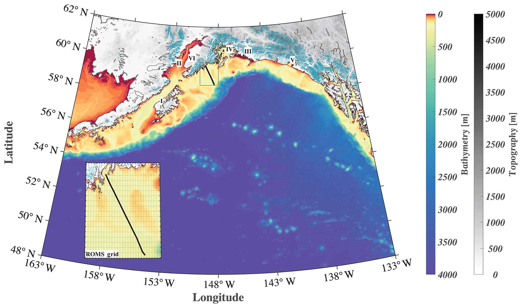
Figure 1Map of the GOA-COBALT model domain showing the depth (m) of the ocean in color and the altitude of the mountains (m) in gray. Glaciated areas are indicated using turquoise coloring of the mountains. The Seward Line is shown using the black line. The inset shows the model mesh and its horizontal resolution of 4.5 km. “I” represents Kodiak Island, “II” represents Cook Inlet, “III” represents Copper River, “IV” represents Prince William Sound, “V” represents Yakutat Bay, and “VI” represents the Kenai Peninsula.
The GOA-LME is especially susceptible to the effects of climate change and ocean acidification. This high-latitude region is naturally low in [] due to the increased solubility of CO2 at low temperatures, the increased vertical mixing of CO2-enriched deep water into the upper water column in winter, riverine and glacial inputs in summer and fall, and the inner shelf dynamics that tend to retain coastal discharges close to shore (Feely and Chen, 1982; Feely et al., 1988; Byrne et al., 2010; Weingartner et al., 2005). The freshwater fluxes into the coastal zone are increasing (Neal et al., 2010; Hill et al., 2015; Hood et al., 2015; Beamer et al., 2016) as this subpolar region continues to warm and deglaciation takes place (Arendt et al., 2002; Larsen et al., 2007; O'Neel et al., 2005). Because glacial meltwater in this region is characterized by low total alkalinity (TA) relative to dissolved inorganic carbon (DIC; Stackpoole et al., 2016, 2017), increasing freshwater discharge pushes the system further towards undersaturation with respect to aragonite. This process likely exacerbates the effects of ocean acidification (Evans et al., 2014).
The GOA-LME is characterized by high concentrations of biologically available dissolved iron (dFe) and low nitrate (NO3) concentrations on the shelf and low dFe and high NO3 concentrations off the shelf (Aguilar-Islas et al., 2015; Wu et al., 2009; Lippiatt et al., 2010; Martin et al., 1989). These two limiting nutrients lead to a phytoplankton community composition dominated by diatoms in the dFe-rich nearshore area and by small phytoplankton in the dFe-poor off-shelf area (Strom et al., 2007). Limited inorganic carbon observations suggest that along with primary productivity and remineralization, physical processes such as downwelling, on-shelf intrusions of deep water, tidal mixing, freshwater discharge, and eddies, are important drivers of the inorganic carbon system dynamics. High biological productivity in spring depresses the partial pressure of carbon dioxide (pCO2) in the water column, resulting in shelf waters supersaturated with respect to aragonite and supporting large fluxes of atmospheric CO2 into the ocean (Fabry et al., 2009; Evans and Mathis, 2013). In September, bottom waters along the shelf are undersaturated with respect to aragonite. This large-scale pattern of aragonite undersaturation is a suggested result of on-shelf intrusion of DIC-rich Pacific basin water near the seafloor and the remineralization of large quantities of organic matter produced during spring blooms (Fabry et al., 2009; Evans et al., 2014). Recent inorganic carbon surveys near marine tidewater glaciers in Glacier Bay, Alaska, and Prince William Sound also suggest that glacial melt water, which is endowed with naturally low total alkalinity (TA), induces seasonal aragonite undersaturation in surface waters (Evans et al., 2014; Reisdorph and Mathis, 2014) and forms corrosive mode water that may subsequently be advected and potentially subducted to distant shelf regions (Evans et al., 2013, 2014).
Insufficient inorganic carbon data coverage impedes our ability to understand the interplay between drivers in different seasons and to determine the relative importance of the various controls of the inorganic carbon system at different locations. Ongoing and historic inorganic carbon system observations in the GOA consist of a limited set of shipboard oceanographic observations, underway measurements from research vessels and scientific sampling systems installed on ferries, and a small number of sensors deployed at fixed nearshore coastal locations (Fabry et al., 2009; Evans and Mathis, 2013; Evans et al., 2014, 2015; Reisdorph and Mathis, 2014; Miller et al., 2018). These draw an incomplete picture of the spatial and temporal variability of the system because the low frequency of the available observations causes aliasing issues. Moreover, because variability is large from seasonal to decadal scales in these waters, the time series from deployed sensors at fixed nearshore locations are not long enough yet to detect an anthropogenic trend in seawater pCO2 and pH (Sutton et al., 2018).
In other shelf systems, regional biogeochemical models have been used to better understand past, present, and future inorganic carbon dynamics and the impacts of climate change and ocean acidification on these ecosystems (Hauri et al., 2013; Turi et al., 2016; Gruber et al., 2012; Franco et al., 2018). Previous regional GOA-LME modeling studies have focused on refining large- and mesoscale circulation features (Dobbins et al., 2009; Xiu et al., 2012), iron limitation (Fiechter and Moore, 2009), and the influence of Ekman pumping (Fiechter et al., 2009) and eddies (Coyle et al., 2012) on the timing and magnitude of the spring bloom. There are only two regional models that simulate the oceanic carbon cycle in the GOA (Siedlecki et al., 2017; Xiu and Chai, 2014). However, neither of these models simulate the influence of freshwater input along the coast, which exhibits high spatiotemporal variability. Siedlecki et al. (2017) used the monthly riverine input climatology by Royer (1982) and applied it equally to the topmost vertical cell along the land mask, whereas Xiu and Chai (2014) did not include riverine input at all. Therefore, to fill gaps in the understanding of the inorganic carbon cycle in the GOA we need a moderately high-resolution model that includes (1) important physical processes such as downwelling, eddies, and cross-shelf fluxes; (2) the carbon cycle; (3) the large spatial and temporal variability of freshwater input; (4) historical simulation long enough to be able to distinguish natural variability from the long-term anthropogenic trend; (5) multiple phytoplankton groups; and (6) iron limitation to reproduce the highly productive nearshore and high-nutrient low-chlorophyll offshore regions.
Here, we introduce a new GOA model that includes a three-dimensional regional ocean circulation model, a complex ecosystem model, and a moderately high-resolution terrestrial hydrological model. We present a thorough model evaluation to test the model's capability to simulate seasonal and interannual inorganic carbon patterns, and we use it to study the seasonal variability and drivers of the inorganic carbon system along the historic Seward Line (Fig. 1). We expand on previous regional modeling efforts by using spatially and temporally variable freshwater forcing; parameterizing freshwater DIC, TA, and nutrients based on available seasonal observations; and conducting a multidecadal hindcast simulation.
2.1 Model setup
We used a GOA configuration of the three-dimensional physical Regional Oceanic Model System (ROMS; Shchepetkin and McWilliams, 2005). ROMS is a free-surface, hydrostatic primitive equation and finite volume (Arakawa C-grid) ocean circulation model. The vertical discretization is based on a terrain-following coordinate system (50 depth levels), with increased resolution towards the surface and the bottom of the ocean. Due to shallower bathymetry, the shelf and coastal areas have higher vertical resolution. For example, in the shallowest areas (depth = 0.5 m), the vertical spacing is 0.01 m, whereas in the deepest water, the vertical spacing is 5 m in surface waters, expanding smoothly to over 300 m near the bottom. The horizontal resolution is eddy-resolving at 4.5 km, which resolves regional coastal upwelling scales. The grid covers a large coastal area from the southern tip of Prince of Wales Island in the southeast to west of Sand Point in the middle of the Aleutian Islands (Fig. 1). The current model configuration is based on Danielson et al. (2016), although with a larger grid extent and a lower horizontal resolution to accommodate the computationally intense ecosystem model. Our GOA-COBALT domain is based on Coyle et al. (2012), although it includes the Alexander Archipelago. Experiments with the Coyle et al. (2012) model have shown that the model had insufficient near-surface vertical mixing, leading to overly fresh water at the surface, which is challenging to mix down. In order to improve on our surface mixing, we added the parameterization of Li and Fox-Kemper (2017). They looked to large-eddy simulations (LESs) to study the effects of unresolved Stokes drift driven by surface waves and the resulting Langmuir circulation on the vertical mixing in a variety of stratification regimes. Their parameterization is now being routinely used in global climate simulations (e.g., Adcroft et al., 2019).
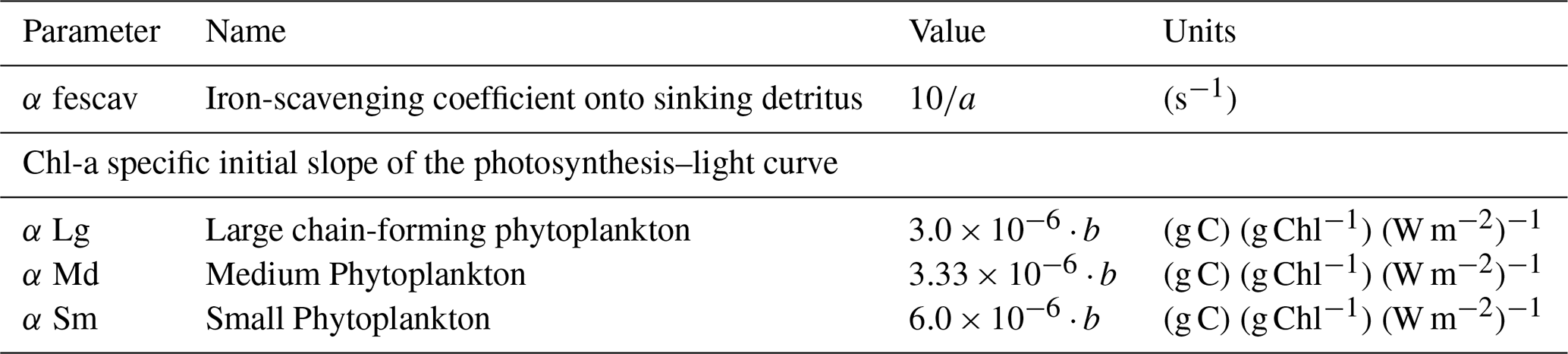
The biogeochemical model used for this study is a modified version of the Carbon, Ocean Biogeochemistry and Lower Trophic (COBALT) marine ecosystem model, which has been applied on a global scale in conjunction with the Earth system model from the Geophysical Fluid Dynamics Laboratory (GFDL) (Stock et al., 2014). Only recently, COBALT was coupled to ROMS and modified with an additional coastal chain-forming diatom to better represent biogeochemical processes and properties in highly productive coastal regions (3PS-COBALT, Van Oostende et al., 2018). 3PS-COBALT resolves the cycles of nitrogen, carbon, phosphate, silicate, iron, calcium carbonate, oxygen, and lithogenic material with 36 state variables. The model contains small phytoplankton that are grazed by microzooplankton; a medium phytoplankton that can be consumed by small copepods; and a larger, chain-forming diatom, which can only be grazed by large copepods and krill. Light, temperature, the most limiting nutrient, and metabolic costs are used to calculate primary productivity for each phytoplankton group. The chlorophyll-to-carbon ratio is dynamic and is based on light (Manizza et al., 2005) and nutrient limitations. Iron limitation depends on an internal cell quota and nitrate and phosphate limitations are simply dependent on their ambient concentrations in the seawater. The currency of biomass and productivity in the model is nitrogen. Organic nitrogen is converted into organic carbon following the Redfield ratio of 106 : 16 (Redfield et al., 1963). DIC and TA are state variables and dictate the inorganic carbon system. Like all other tracer concentrations in the model, these two variables are affected by diffusion, horizontal and vertical advection, and sources minus sink terms that include net primary production, CaCO3 formation and dissolution both in the water column and sediments, detritus remineralization in the water column and sediments, zooplankton respiration, and atmosphere–ocean CO2 fluxes. The Chl-a-specific initial slope of the photosynthesis–light curve and the iron-scavenging coefficient onto sinking detritus were both adjusted to better represent the GOA biogeochemistry and ecosystem (Table 1). All other constants are based on Van Oostende et al. (2018).
Table 1Summary of the definitions, abbreviations, values, and units of the model parameters adjusted from Van Oostende et al. (2018) to better represent the ecosystem in higher northern latitudes (Strom et al., 2010). , and b=4.5998.
2.2 Initial conditions, boundary conditions, and forcing
Physical initial and boundary conditions for currents, ocean temperature, salinity, and sea surface height were taken from the Simple Ocean Data Assimilation ocean/sea ice reanalysis 3.3.1 (SODA, Carton et al., 2018, available as 5-day averages). After a model spin-up of 10 years, the hindcast simulation (1980 to 2013) was forced at the surface with 3-hourly winds, surface air temperature, pressure, humidity, precipitation, and radiation from the Japanese 55-year Reanalysis (JRA55-do) 1.3 project (Tsujino et al., 2018). The atmospheric fields were used to compute surface stresses and fluxes using a bulk flux algorithm (Large and Yeager, 2008). Precipitation was solely counted as a negative salt flux and did not change any volume or dilute any other tracers, such as DIC and TA. Along its coastal boundary, freshwater was brought in from numerous rivers and tidewater glaciers. This was done with a point-source river input via exchange of mass, momentum, and tracers through the coastal wall at all depths (Danielson et al., 2020). A hydrological model provided riverine input at a 1 km resolution and at a daily time step (Beamer et al., 2016). The hydrological model was based on a suite of weather, energy balance, snow/ice melt, soil water balance, and runoff routing models forced with Climate Forecast System Reanalysis data (Saha et al., 2010). The reanalysis data were regridded from their 0.2 degree resolution to the 1 km hydrological model grid using MicroMet (Liston and Elder, 2006). Nutrient, DIC, and TA concentrations in the freshwater were based on available observations and are summarized in Table 2. As found in other freshwater data (Rheuban et al., 2019), DIC concentrations were higher than TA, showing that the freshwater discharging into the GOA is quite acidic (Stackpoole et al., 2016, 2017).
(Stackpoole et al., 2016, 2017)(Stackpoole et al., 2016, 2017)Aguilar-Islas et al. (2015)(Hood and Berner, 2009)(Fellman et al., 2015)Table 2Table listing riverine dissolved inorganic carbon, total alkalinity, nitrate, dissolved iron, dissolved oxygen, and temperature values. When seasonal observations were available, the variables followed a seasonal cycle. These variables are listed with their minimum, mean, and maximum levels. The values of all other variables were initialized at a very small number (<0.0001).

* Aguilar-Islas et al. (2015) observed a maximum of 10 nmol kg−1 dFe in nearshore waters with a salinity of 25. In order to model high nearshore dFe values (see Fig. 2), riverine dFe was set to 30 nmol kg−1.
DIC and TA initial conditions for the hindcast simulation were extracted from the mapped version 2 of the Global Ocean Data Analysis Project (GLODAPv2.2016b, Lauvset et al., 2016) data set. GLODAP DIC data, which were referenced to 2002, were normalized to 1980 using the anthropogenic CO2 estimates for the GOA by Carter et al. (2017). Carter et al. (2017) suggest two different rates of the depth-dependent increase of anthropogenic CO2 per year for the period from 1980 to 1999 and for the period from 2000 to the present. The anthropogenic CO2 increase for the corresponding time period was added (or subtracted) in monthly increments from the reference year. A seasonal cycle was added to the surface based on Takahashi et al. (2014). Following Hauri et al. (2013), DIC and TA were assumed to vary throughout the upper 200 m of the water column, but they were attenuated proportional to the seasonal variations of temperature across depth. Each year, DIC boundary conditions increased as a result of anthropogenic CO2 increase, following estimates for the region made by Carter et al. (2017). Nitrate, phosphate, oxygen, and silicate initial conditions were taken from the World Ocean Atlas 2013 (Garcia et al., 2013). All other variables were initialized based on a climatology from a GFDL-COBALT simulation (1988–2007) forced by Common Ocean-ice Reference Experiment (CORE-II) data, as described in Stock et al. (2014). Atmospheric pCO2 was forced with monthly means derived from the Mauna Loa CO2 record (https://www.esrl.noaa.gov/gmd/ccgg/trends/data.html, last access: 22 January 2018).
3.1 Physics
The model domain is strongly influenced by freshwater coming from hundreds of glacier-fed rivers and tidewater glaciers that ring the GOA. Our approach of using a hindcast simulation from a highly resolved land hydrography model (Beamer et al., 2016) to force the freshwater input was recently evaluated through comparison to salinity, temperature, velocity, and dynamic height observations (Danielson et al., 2020). The findings of Danielson et al. (2020) are summarized in the following paragraph. The influence of the springtime freshet is well reproduced by the model, with low salinities (∼26 PSU) in the nearshore upper 10–20 m of the water column (r∼0.5–0.6, p∼0.05). While the correlation between salinity observations and model output is only slightly weaker in summertime, the model has difficulty in reproducing small-amplitude salinity variations between October and March, when riverine input is lowest and the signal-to-noise ratio of salinity is small. Temperature is particularly well modeled in the first half of the year, with the highest correlations (r∼0.9, p<0.05) in the middle of the water column. The model is also able to skillfully reproduce monthly dynamic height anomalies in summer, fall, and winter (not shown). Overall, the freshwater fluxes used in this study are more realistic than in previous studies because they are derived from a temporally and spatially highly resolved hindcast simulation forced with meteorological reanalysis data sets. Compared with previous studies (Royer, 1982; Wang et al., 2004; Hill et al., 2015; Siedlecki et al., 2017), this current model configuration is better able to reproduce low salinity levels in coastal areas across the GOA and can, therefore, more adequately reproduce the Alaska Coastal Current (Danielson et al., 2020).
3.2 Nutrients and Chl-α
High concentrations of biologically available dFe prevail across the inner to mid GOA shelf due to the dFe-rich input of glacially fed rivers (Aguilar-Islas et al., 2015; Wu et al., 2009; Lippiatt et al., 2010). While these shelf areas are low in NO3, they border the NO3-rich and dFe-poor waters off the shelf (Martin et al., 1989). The spatial variability of these two limiting nutrients orchestrate the phytoplankton community composition, with diatom-dominated areas in the dFe-rich nearshore environment and small phytoplankton in dFe-depleted offshore areas (Strom et al., 2010). Here, we first evaluate the modeled spatial variability of surface dFe, NO3, and Chl-α by comparing them to in situ and satellite observations (Aguilar-Islas et al., 2015; Lippiatt et al., 2010; Crusius et al., 2017; MODIS-Aqua Ocean Color Data, NASA Goddard Space Flight Center, Ocean Ecology Laboratory, 2014).
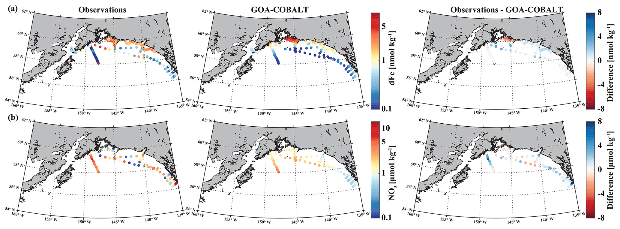
Figure 2Observed (left) and GOA-COBALT-simulated (middle) surface dissolved iron (a, dFe, nmol kg−1) and nitrate (b, NO3, µmol kg−1) concentrations. The right panel shows the difference between the observed and modeled (a) dFe and (b) NO3. The observations were made in July, August, and September (Aguilar-Islas et al., 2015; Lippiatt et al., 2010; Crusius et al., 2017). The model output is based on a mean of modeled July, August, and September values from a 1980 to 2013 climatology. dFe and NO3 are plotted on a log scale.
dFe observations along a transect near the Copper River estuary suggest that coastal surface concentrations can reach up to 9.4 nmol kg−1 in mid to late summer west of Prince William Sound (Fig. 2a), when glacial melt and riverine input are highest. These surface concentrations decrease rapidly with distance from shore, with levels of <1 nmol kg−1 near the shelf break and beyond. The horizontal surface dFe gradient across the shelf, with high dFe concentrations in coastal areas and dFe levels near depletion offshore, was simulated well by the model. For example, the model shows dFe values of up to 8 nmol kg−1 (Fig. 2a) in some coastal areas and low concentrations (<0.5 nmol kg−1) at the shelf break. Overall, the model slightly underestimates dFe along the coast, except for the area surrounding Copper River and near the shelf break, despite the relatively high dFe riverine boundary condition (Table 2).
The low observed surface summertime values of NO3 in coastal areas are simulated well by the model. Observed NO3 values range up to 5.4 µmol kg−1 (with the exception of a few outliers in southeast Alaska), and modeled surface NO3 concentrations reach a maximum of 4.3 µmol kg−1 (Fig. 2b).
The modeled spring phytoplankton bloom starts in April and coarsely matches with the timing of the satellite-observed spring bloom (Fig. 3). Simulated surface Chl-α then ranges between 3 and 4 µg kg−1 across the entire shelf, with some nearshore areas reaching surface Chl-α levels of 5 µg kg−1. However, satellite images suggest that Chl-α concentrations are more patchy in April than shown by the model, with lower concentrations across the shelf (1–2 µg kg−1). While peak observed Chl-α concentrations between 7 and 9 µg kg−1 are localized in southeast Alaska in May, simulated Chl-α levels of 5 µg kg−1 are more widespread along the coast, with peak concentrations of 6 to 7 µg kg−1 in some select areas. In July through August, simulated Chl-α levels slowly taper off, although some nearshore areas still reach peak concentrations of 6 µg kg−1. In September, on-shelf modeled Chl-α concentrations are <3 µg kg−1. In summary, observed Chl-α concentrations are lower than suggested by the model across the shelf and the domain throughout the summer. With the exception of November through February, when modeled Chl-α concentrations are <1 µg kg−1, standing stock Chl-α concentrations are also overestimated by a factor of 2 by the model throughout the year.
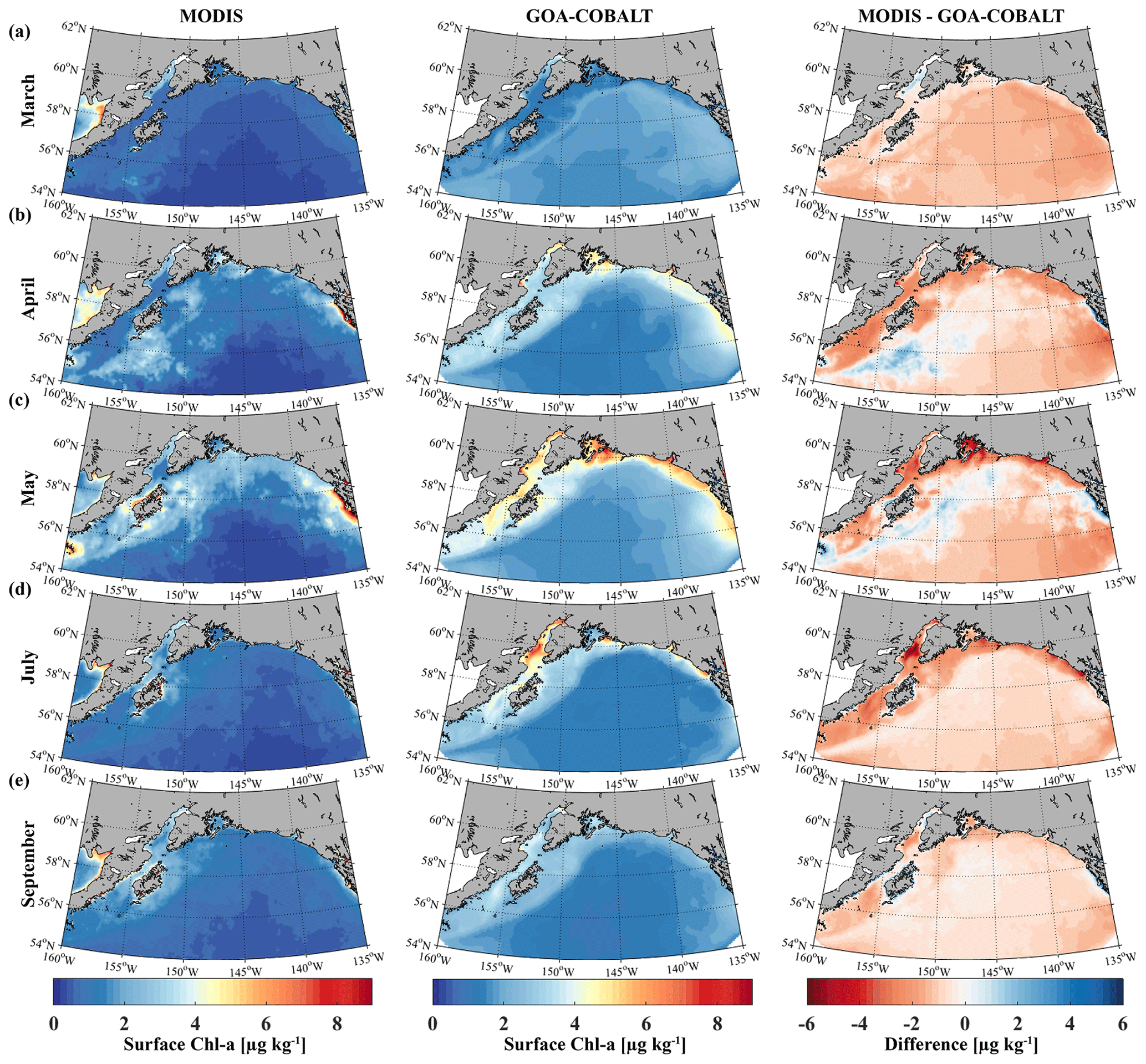
Figure 3Monthly climatology (1980–2013) for satellite-based (left, MODIS) and GOA-COBALT-simulated (middle) surface Chl-α concentrations for (a) March, (b) April, (c) May, (d) July, and (e) September. The right panel shows the difference between MODIS and GOA-COBALT surface Chl-α concentrations. (Source for MODIS data: MODIS-Aqua Ocean Color Data, NASA Goddard Space Flight Center, Ocean Ecology Laboratory, 2014.)
3.3 Model skill to simulate spring and fall oceanographic conditions
Inorganic carbon observations in the GOA have been collected every spring and fall along the historic Seward Line since 2008 (Evans et al., 2013). Here, we compare May and September monthly means of our 2008–2012 model output to the publicly available shipboard observations made in May and September of the corresponding years. To do so, the model output was sampled at the closest grid point to every Seward Line station. The model output and observations were then interpolated onto the same grid and averaged across all years for May and September.
In May, observations and model output clearly show the influence of freshwater on the coastal water properties, including inorganic carbon chemistry (Fig. 4). In nearshore surface areas, waters are cold, fresh, and low in TA and DIC. The influence of freshwater is visible throughout the transect but with slowly increasing values of salinity, DIC, and TA with distance from the coast. The model generally reproduces these patterns well, although with slightly higher values for all three parameters across the transect. For example, observed surface salinity ranges between 31.4 at 59.8∘ N and 32.2 at the end of the transect (Fig. 4b). TA varies between 2143 and 2170 µmol kg−1, and DIC varies between 1965 and 2017 µmol kg−1 (Fig. 4c, d). Simulated ranges of these parameters are similar (salinity from 31.7 to 32.4, TA from 2163 to 2203 µmol kg−1, and DIC from 2009 to 2038 µmol kg−1). The largest biases in salinity (Sbias=0.6), alkalinity (TAbias=35 µmol kg−1), and DIC (DICbias=46 µmol kg−1) are found around 59.6∘ N. The overestimation of salinity suggests that the freshwater influence is overly weak, leading to the modeled overestimation of TA and DIC. However, the bias in DIC relative to the bias in TA is largest in the grid cell closest to the coast, which leads to an underestimation of modeled pH and Ωarag of up to 0.09 and 0.29, respectively (Fig. 4e, f). The bias of surface pH and Ωarag vanishes with distance from the coast. The larger difference in DIC relative to TA near the coast is likely due to an underestimation of biological carbon drawdown, leading to the underestimation of pH and Ωarag in nearshore surface waters. At depth farther offshore, salinity-, DIC-, and TA-enriched waters are visible on the shelf. As a result, the springtime in situ aragonite saturation horizon (depth where Ωarag=1) is shallower offshore than nearshore (Fig. 4f). Observations suggest that with a depth of the aragonite saturation horizon of about 200 m, the seafloor on the shelf up to 59.1∘ N is undersaturated with respect to aragonite. The model underestimates the aragonite saturation horizon depth slightly. However, because the model's bathymetry is shallower than the observed depth at this particular location (gray areas in Fig. 4), modeled bottom water masses across the shelf are not undersaturated with respect to Ωarag north of 59∘ N.

Figure 4Visual comparison of vertical sections of (a) temperature (∘C), (b) salinity, (c) total alkalinity (TA, µmol kg−1), (d) dissolved inorganic carbon (DIC, µmol kg−1), (e) pH, and (f) the aragonite saturation state (Ωarag) of climatologies (2008–2012) of observations made along the Seward Line in May (left, Evans et al., 2013), the corresponding monthly model output (middle), and the difference between observed and GOA-COBALT-simulated variables (right). The model output was sampled at locations where observations were made. Observations and model points were then vertically and horizontally interpolated onto the same grid and averaged across the years 2008 to 2012. The gray area depicts the observed sampling depth in the left panel and the seafloor in the model output. The black line in panel (f) indicates Ωarag=1.
In September, nearshore surface waters are warm (∼ 11 ∘C) and much fresher than in spring (Fig. 5a, b). The observed surface salinity is as low as 27.6 at 59.8 ∘C and increases to 32 salinity units at the end of the transect. Modeled surface salinity ranges between 26.3 and 31.8. It is important to note that observed surface salinity at the station closest to the coast is also as low as 26.8, but it is masked out in this point-by-point comparison. As a result of this bias in salinity, modeled nearshore TA and DIC concentrations in the upper 30 m are underestimated by ∼30 and ∼20 µmol kg−1, respectively (Fig. 5c, d). Because the model is likely underestimating the magnitude of late-season phytoplankton blooms, the bias in DIC is slightly smaller than in TA. Modeled Ωarag underestimates observations by <0.2 in this area (Fig. 5f). At depth, the model output aligns well with observations. Both observations and model output suggest that bottom waters across the Seward Line transect are undersaturated with respect to aragonite in fall. Observations also show an intermediate maximum in DIC at about 150 m depth, which leads to an even shallower aragonite saturation horizon (Fig. 5d). This small-scale feature may be due to remineralization at mid depth and is not simulated by the model. Overall, the model does a reasonable job of simulating the spatial patterns of salinity, TA, DIC, pH, and Ωarag in spring and fall, with statistically significant (p value < 0.05) Pearson correlation coefficients of between 0.82 and 0.97 (Fig. 6a, b). The model overestimates springtime temperature along the surface and around 100 m offshore, which is reflected in a slightly lower Pearson correlation coefficient of 0.62. The Pearson correlation coefficients (Pcc) and their corresponding p values were calculated based on the climatologies presented in Figs. 4 and 5. All standard deviations and correlation coefficients between the observed and modeled variables are summarized using Taylor Diagrams in Fig. 6.
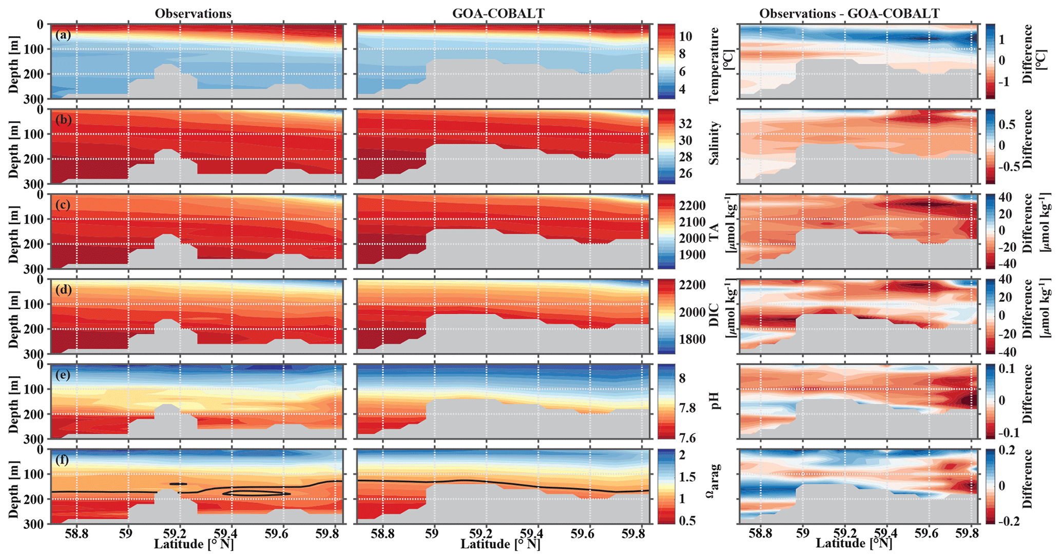
Figure 5Visual comparison of vertical sections of (a) temperature (∘C), (b) salinity, (c) total alkalinity (TA, µmol kg−1), (d) dissolved inorganic carbon (DIC, µmol kg−1), (e) pH, and (f) the aragonite saturation state (Ωarag) of climatologies (2008–2012) of observations made along the Seward Line in September (left, Evans et al., 2013), the corresponding monthly model output (middle), and the difference between observed and GOA-COBALT-simulated variables (right). The model output was sampled at locations where observations were made. Observations and model points were then vertically and horizontally interpolated onto the same grid and averaged across the years 2008 to 2012. The gray area depicts the observed sampling depth in the left panel and the seafloor in the model output. The black line in panel (f) indicates Ωarag=1.

Figure 6Taylor diagrams (Taylor, 2001) of model-simulated temperature, salinity, total alkalinity (TA, µmol kg−1), dissolved inorganic carbon (DIC, µmol kg−1), pH, and the aragonite saturation state (Ωarag) compared to observations made along the Seward Line in (a) May and (b) September across the upper 300 m (Figs. 4, 5). Climatologies of the averaged modeled monthly means of May and September are compared to climatologies of observed conditions during spring and fall cruises in the years 2008 through 2012. The distance from the origin is the normalized standard deviation of the modeled parameters. The azimuth angle shows the correlation between the observations and the modeled output, whereas the distance between the model point and the red observation point shows the normalized root mean square misfit between the modeled and observed data.
3.4 Model skill to simulate interannual variability
The GOA oceanography undergoes large interannual to decadal variability as a result of the El Niño–Southern Oscillation (ENSO), the Pacific Decadal Oscillation (PDO), and other climate modes of variability that drive changes in freshwater flux, water temperature, and winds (Whitney and Freeland, 1999; Hare and Mantua, 2000). These physical changes are likely translated into the inorganic carbon chemistry. Here, we investigate the model's skill to simulate interannual features, comparing Hovmöller plots of observations made in May and September between 2008 and 2012 and modeled monthly means of the corresponding time and location for temperature, salinity, TA, and DIC (Figs. 7, 8). We also calculate the monthly observed and modeled anomalies for May and September, based on the observed and modeled 5-year monthly mean of each variable (Figs. 9, 10). In the following, we will describe observations of years that stand out within this 5-year record and determine whether these features were captured by the model.
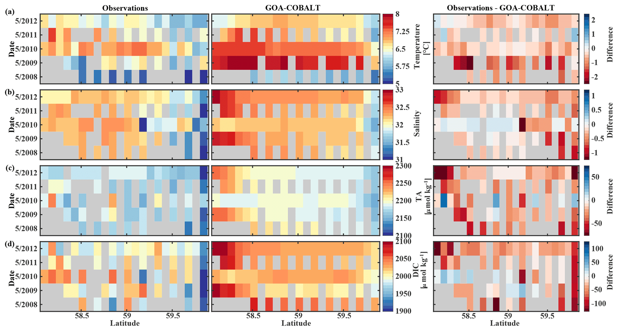
Figure 7Hovmöller plots showing the observed (left) and modeled monthly mean (right) surface (a) temperature (∘C), (b) salinity, (c) total alkalinity (TA, µmol kg−1), and (d) dissolved inorganic carbon (DIC, µmol kg−1) in May along the Seward Line between 2008 and 2012. Gray areas show missing data.
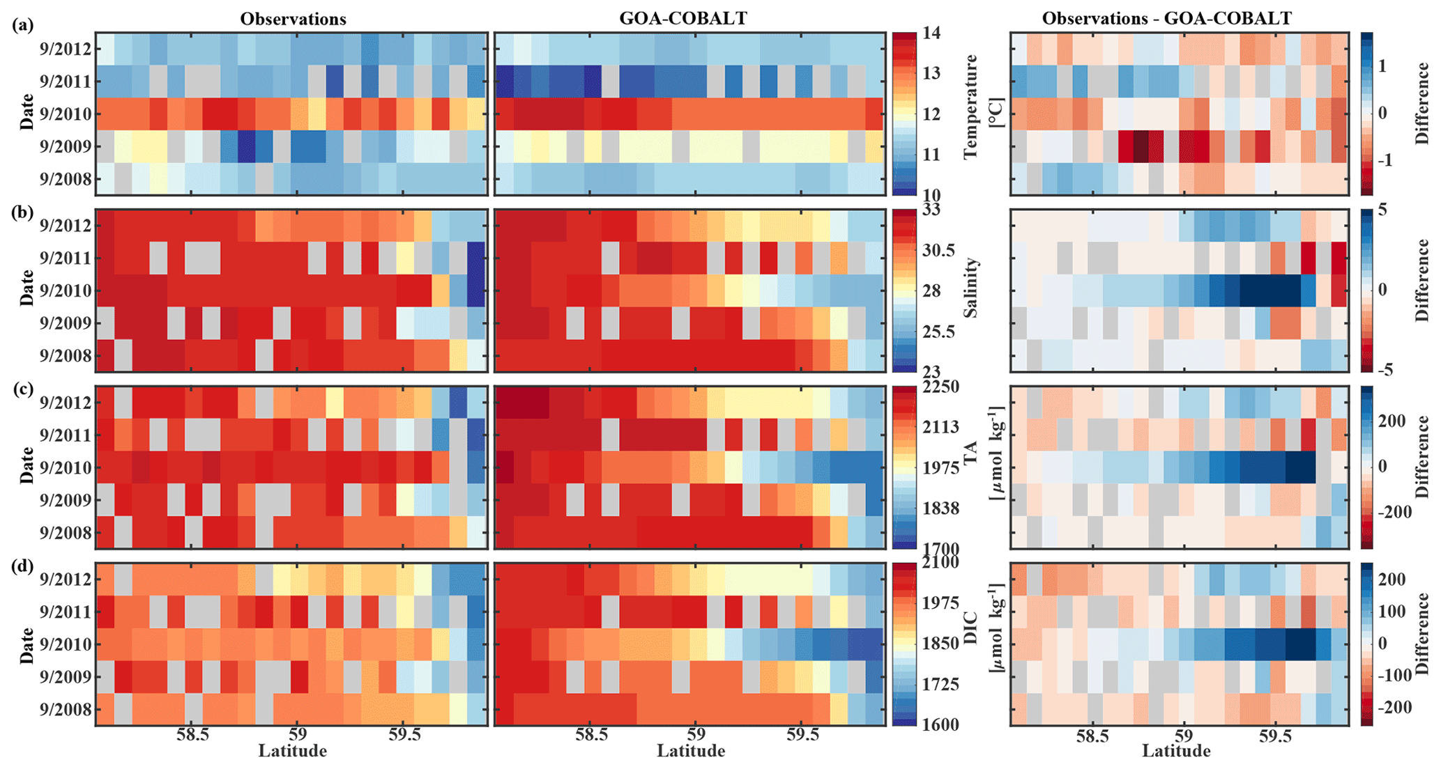
Figure 8Hovmöller plots showing the observed (left) and modeled monthly mean (right) surface (a) temperature (∘C), (b) salinity, (c) total alkalinity (TA, µmol kg−1), and (d) dissolved inorganic carbon (DIC, µmol kg−1) in September along the Seward Line between 2008 and 2012. Gray areas show missing data.
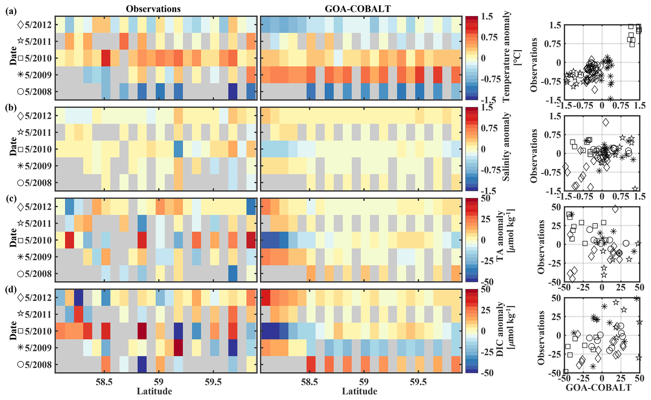
Figure 9Hovmöller plots showing the observed (left) and modeled (center) monthly anomalies from the 5-year mean (2008–2012) of surface (a) temperature (∘C), (b) salinity, (c) total alkalinity (TA, µmol kg−1), and (d) dissolved inorganic carbon (DIC, µmol kg−1) in May along the Seward Line. Gray areas show missing data. The right column shows plots of observed vs. modeled monthly anomalies for the corresponding parameter. Different marker types are used to indicate different years. The marker legend is given in the left column. The root mean square error (RMSE), the Pearson correlation coefficient (Pcc), and the p value for the observed and modeled interannual monthly anomalies are listed in Table 3.

Figure 10Hovmöller plots showing the observed (left) and modeled (center) monthly anomalies from the 5-year mean (2008–2012) of surface (a) temperature (∘C), (b) salinity, (c) total alkalinity (TA, µmol kg−1), and (d) dissolved inorganic carbon (DIC, µmol kg−1) in September along the Seward Line. Gray areas show missing data. The right column shows plots of observed vs. modeled monthly anomalies for the corresponding parameter. Different marker types are used to indicate different years. The marker legend is given in the left column. The root mean square error (RMSE), the Pearson correlation coefficient (Pcc), and the p value for the observed and modeled interannual monthly anomalies are listed in Table 3.
The observed and modeled springtime surface temperatures show large interannual variability (Figs. 7a, 9a). Within the 5-year-long record, 2008 was a particularly cold spring, with surface temperatures of around 5 ∘C. The model also simulated May 2008 as the coldest spring, but it overestimated the temperature by approximately 1 ∘C. In May 2010, observed sea surface temperatures were particularly high (> 6 ∘C) across the shelf, which was well reflected by the model. While the model also suggested high temperatures in the previous spring, the observations do not show a particularly warm spring in 2009. The modeled and observed interannual variability of surface temperatures in May are statistically significantly correlated with a Pcc of 0.54 (Table 3). The interannual variability in salinity is visible by how far the freshwater penetrates into the open ocean. For example, observations suggest that freshwater penetrated farther offshore in 2010 than in other years (Fig. 7b), which was not reflected by the model.
Table 3Table listing the root mean square error (RMSE), the Pearson correlation coefficient (Pcc), and the p value between the observed and modeled interannual variability at the surface. The RMSE, Pcc, and the corresponding p value were based on observed and modeled monthly anomalies from a temporal mean of May or September (2008–2012) along the Seaward Line transect. Statistically significant Pcc values and the corresponding p values are indicated in bold. The anomalies are shown in Figs. 9 and 10.
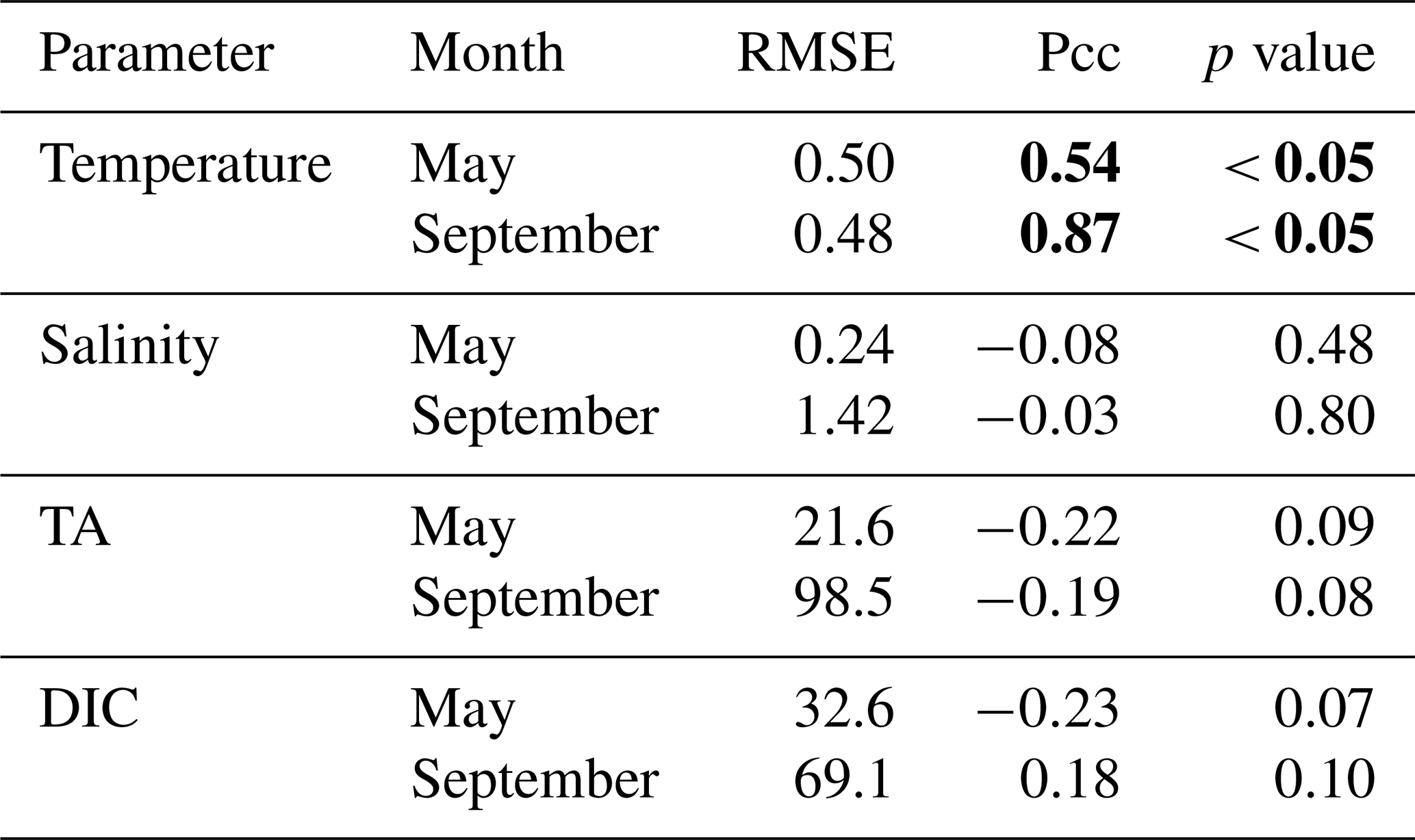
The anomalous warm sea surface temperatures observed in spring 2010 remained persistent into fall, with temperatures around 13 ∘C across the whole transect (Figs. 8a, 10a). This anomalously warm fall was well simulated by the model. Overall, the modeled interannual variability of fall surface temperatures correlated well with the observations (Pcc = 0.87, ). Interestingly, in the anomalously warm fall of 2010, observations suggest anomalously high salinities penetrating closer to the nearshore than in other years, which was not reflected by the model (Figs. 8b, 10b). However, observed lower salinities mid transect in 2012 were also simulated by the model, which directly translated into TA and DIC (Fig. 8c, d). Overall, there was no clear interannual pattern in observed or simulated salinity, TA, and DIC between 2008 and 2012 (panels b–d in Figs. 7–10), and no statistically significant correlation between the observed and modeled spring and fall anomalies (Table 3).
The historic Seward Line time series gives insights into the inorganic carbon dynamics in May and September. Here, we use our model output to explore other months of the year that are not covered by inorganic carbon observations (Fig. 11). The lowest surface temperatures of <3 ∘C are found nearshore in February and March (not shown). In spring, surface waters slowly warm, reaching an annual maximum in July/August, when surface temperatures are >13 ∘C. The highest nearshore surface salinities () are observed in late winter, which decrease to 24 salinity units between August and October, when the influence of freshwater is strongest. The freshwater also decreases surface TA and DIC to their lowest respective levels of 1625 and 1500 µmol kg−1 in August. The additional biologically driven decrease in DIC between April and June, when surface Chl-α concentrations (up to 7 µg kg−1) are highest, leads to relatively high pH (8.13) and Ωarag (2.05), despite the freshwater influence and its diluting character. Once phytoplankton blooms begin to taper off in July and August, DIC slowly increases relative to TA, leading to a decrease in Ωarag to a low of 1.21 and a pH of 8.05 in October. Ωarag remains <1.5 across the whole water column between January and March. In April, the incoming light and nutrient concentrations are sufficient again to trigger phytoplankton blooms that slowly decrease DIC and, in turn, increase Ωarag and pH.
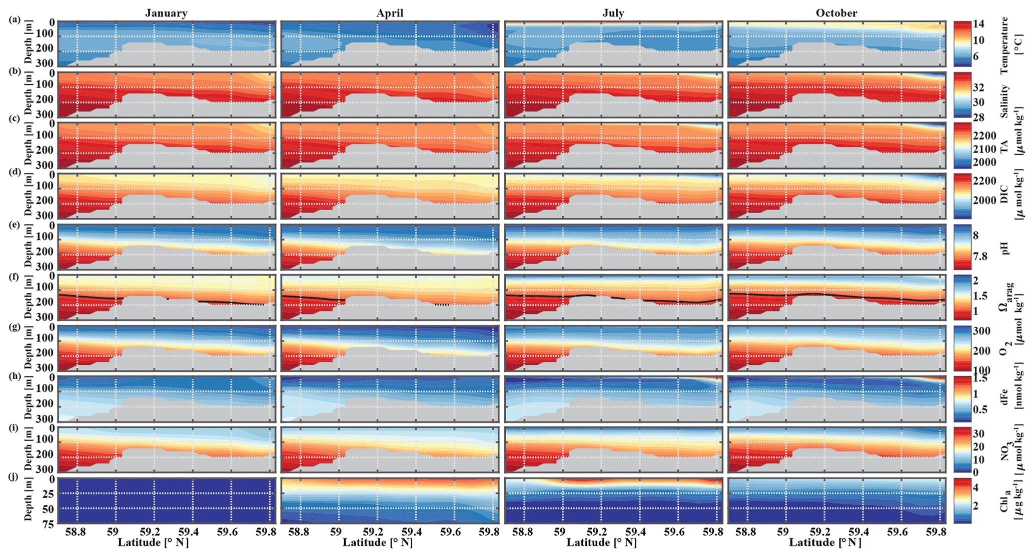
Figure 11Seward Line transect of modeled (a) temperature (∘C), (b) salinity, (c) total alkalinity (TA, µmol kg−1), (d) dissolved inorganic carbon (DIC, µmol kg−1), (e) pH, (f) aragonite saturation state (Ωarag), (g) dissolved oxygen (DO, µmol kg−1), (h) dissolved iron (FE, nmol kg−1), (i) nitrate (NO3, µmol kg−1), and (j) Chl-α (µg kg−1) in January, April, July, and October (averaged across 2008–2012). Note that Chl-α is only plotted across the upper 75 m of the water column. The black solid line in row (f) indicates Ωarag=1. The gray areas indicate the seafloor.
Starting in May, downwelling relaxes and more saline and DIC-rich waters intrude onto the shelf, leading to maximum bottom salinities and DIC concentrations of and DIC µmol kg−1, respectively, on the shelf. The relaxation of downwelling results in aragonite undersaturation of bottom waters across the transect between June and January. The destruction of organic matter and remineralization additionally increase DIC between June and September and, therefore, further enhance aragonite undersaturation (Fig. 12b). The onset of downwelling in September typically starts the annual decrease in near-bottom shelf salinity and DIC (increase of Ωarag and pH) levels, which reach their respective minimums in late winter or spring.
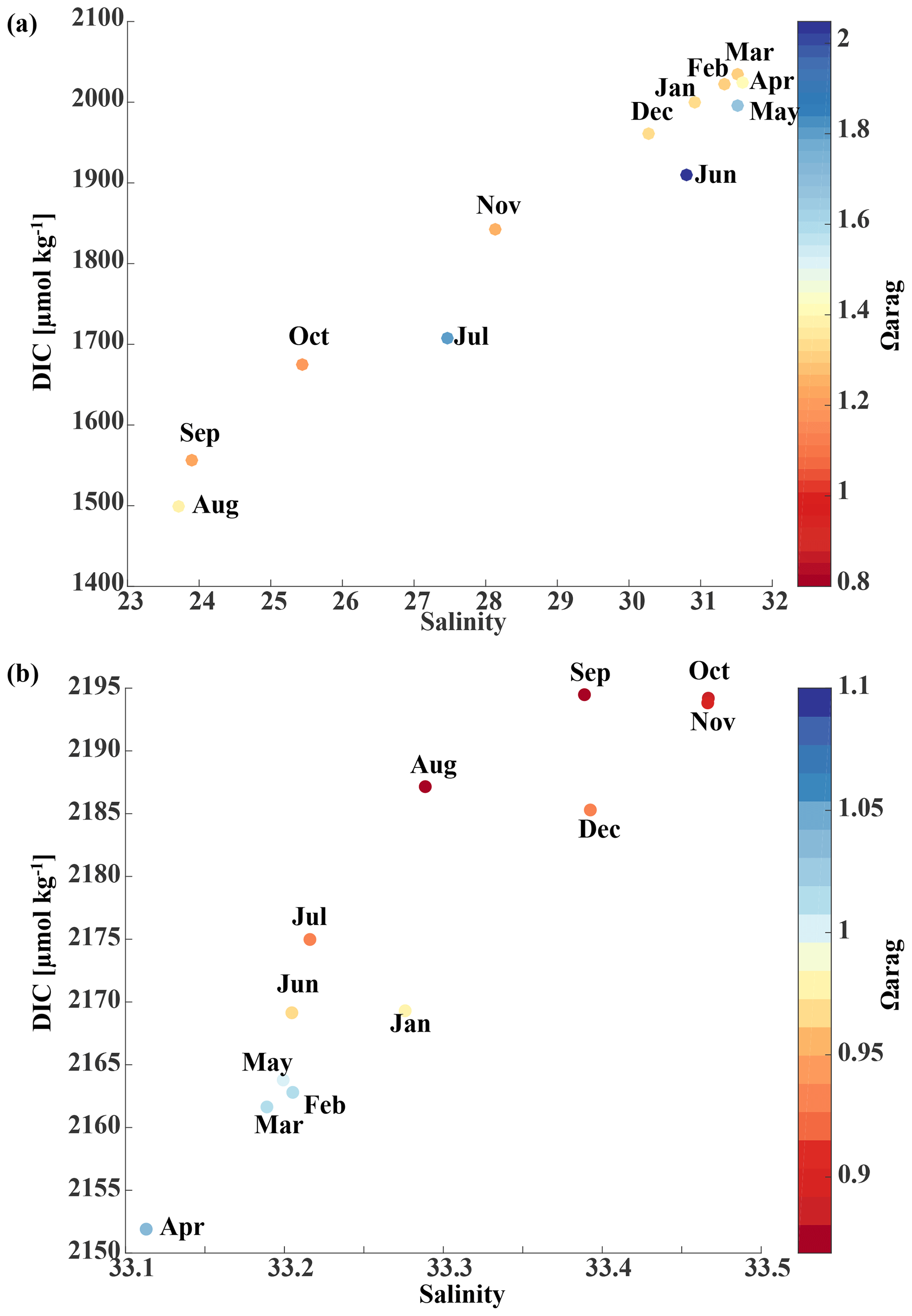
Figure 12Modeled salinity vs. dissolved inorganic carbon (DIC, µmol kg−1) as a function of Ωarag and month (a) at the surface and grid cell closest to the coast and (b) on the seafloor at 59.2∘ N along the Seward Line. Note that the color bars and axes are on different scales.
Glacial freshwater is the most important driver of the nearshore inorganic carbon dynamics of the GOA in summer and fall. We further investigate the influence of coastal dilution from the rather acidic TA and DIC freshwater end-member (Table 2) on surface Ωarag, pH, and pCO2. Following the step-by-step description in Rheuban et al. (2019), we used a linear Taylor decomposition to separate and analyze the controlling factors of the variability in surface Ωarag, pH, and pCO2. Offshore mixing end-members of Ωarag, pH, and pCO2 were determined from offshore DIC and TA in April and August with CO2sys.m (Lewis and Wallace, 1998; van Heuven and Wallace, 2011) and were used as reference values. All calculations are based on the dissociation constants of Lueker et al. (2000) and the KHSO4 and total boron–salinity formulations of Dickson (1990) and Dickson (1974), respectively. Anomalies from the reference value were calculated for each grid cell using a linear Taylor series decomposition, adding up the thermodynamic effects of temperature and salinity, the perturbations due to biogeochemistry, and conservative mixing with freshwater DIC and TA end-members. For a more detailed description of the methodology, the reader is referred to Rheuban et al. (2019). We focus our analysis on April and August because these 2 months are the least and most affected by freshwater, respectively. Figure 13 shows mixing diagrams of surface Ωarag, pH, and pCO2 vs. salinity from an area starting at the Kenai Peninsula to south of Yakutat Bay. Note that the plots show the effects of salinity changes and biogeochemistry on surface Ωarag, pH, and pCO2 as well as seasonal differences in temperature and in the offshore and freshwater end-members, DIC and TA. The shaded areas in Fig. 13c and d show the additive effects of salinity and dilution with seasonally varying DIC and TA freshwater end-members, as calculated with the linear Taylor expansion. The gray area in Fig. 13c accounts for variability in DIC and TA mixing curves between January and April and in Fig. 13d for DIC and TA variability between April and August. Deviations from the shaded area are driven by biogeochemistry and temperature.
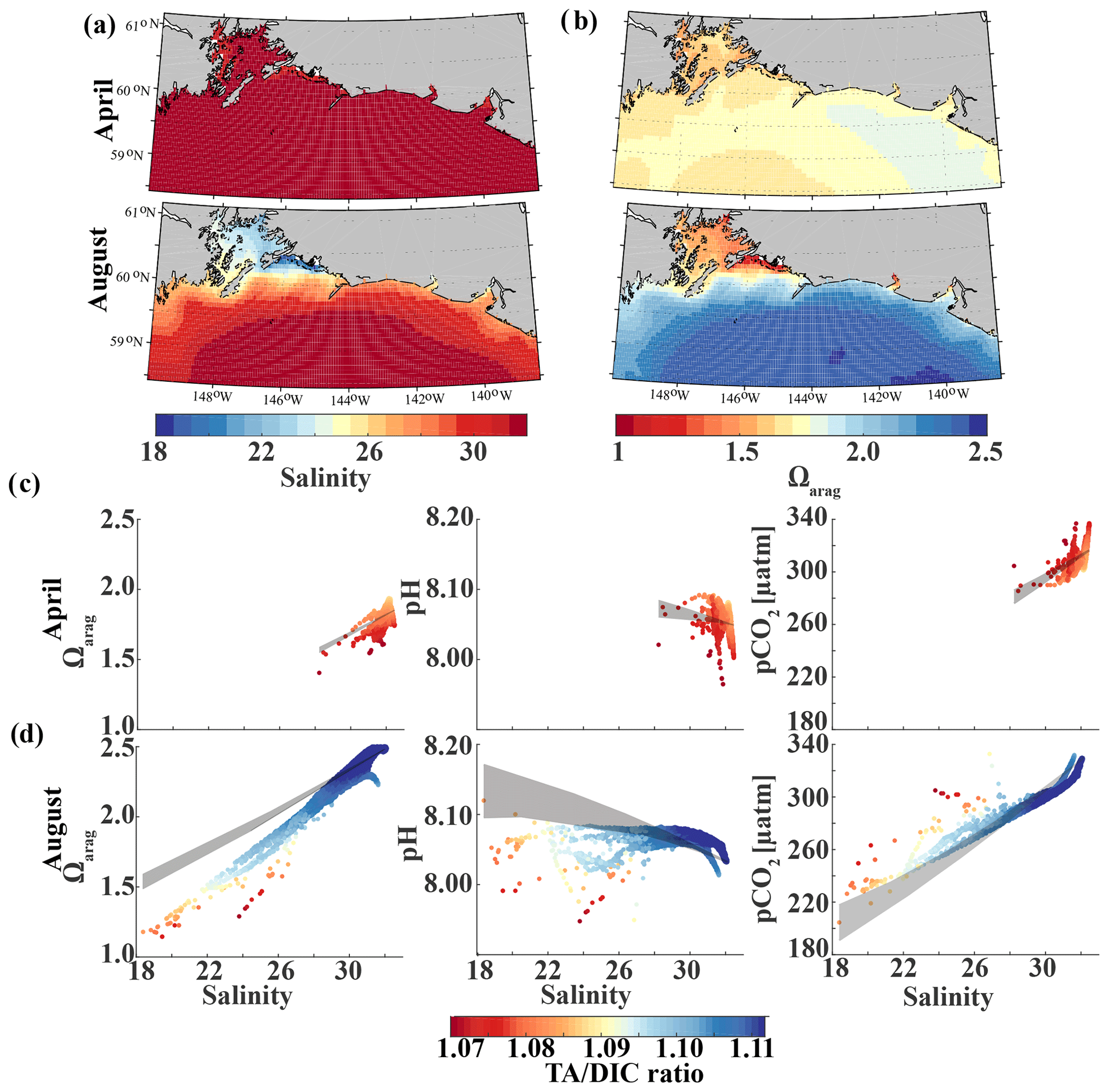
Figure 13Map of the climatological mean (1980–2013) of (a) surface salinity and (b) surface Ωarag in April (top) and August (bottom). Plots of surface Ωarag (left), pH (middle), and pCO2 (µatm) (right) vs. salinity as a function of the TA∕DIC ratio in (c) April and (d) August. The shaded area indicates the range of Ωarag, pH, and pCO2, respectively, based on the assumption that changes in the respective variable only arise from variations in salinity and from the dilution effect of freshwater on DIC and TA.
In April, surface salinity is >30, with the exception of a few nearshore spots in Prince William Sound and Yakutat Bay, where surface salinity can decrease to 28 salinity units (Fig. 13a). Surface Ωarag ranges between 1.5 and 1.85, pH varies between 8.08 and 8.10, and pCO2 ranges between 280 and 340 µatm (Fig. 13b, c).
In August, surface salinity can be as low as 18 in Prince William Sound and near Copper River, with a strong salinity gradient increasing in the offshore direction, reaching salinities >32 offshore (Fig. 13a). Surface Ωarag ranges between 1.14 and 2.5, pH varies between 8.07 and 8.16, and pCO2 ranges between 205 and 333 µatm, reflecting the influence of freshwater in late summer (Fig. 13d). The linear Taylor decomposition indicates that decreasing salinity increases both Ωarag and pH, whereas mixing with low TA and DIC freshwater end-members decreases Ωarag and pH (Fig. 14a, b). The increase in pH due to decreasing salinity is much stronger than for Ωarag, thereby canceling or even counteracting (depending on the freshwater end-member) the decrease in pH due to mixing. Thus, the influence of salinity on pH works to counteract the influence of low TA and DIC freshwater end-members on pH such that the observed pH exhibits no correlation with the observed salinity. Ωarag is more strongly affected by mixing than by salinity, resulting in a decrease in Ωarag of about 1 unit. In contrast to Ωarag and pH, decreasing salinity strongly decreases pCO2, which is counteracted to some degree by an increase in pCO2 due to mixing with low TA and DIC end-members and respiration (Fig. 14c). Therefore, the additive effects of salinity and mixing with low TA and DIC freshwater lead to a decoupling of Ωarag, pH, and pCO2. Deviations from the shaded areas in Fig. 13d are mainly driven by biogeochemistry, which decreases Ωarag and pH and increases pCO2 as a result of net respiration during August. Temperature effects are small for Ωarag and pH, whereas the negative effect of decreasing temperature is similar to the negative effect of mixing with low TA and DIC freshwater end-members for pCO2, enhancing a decrease in pCO2.
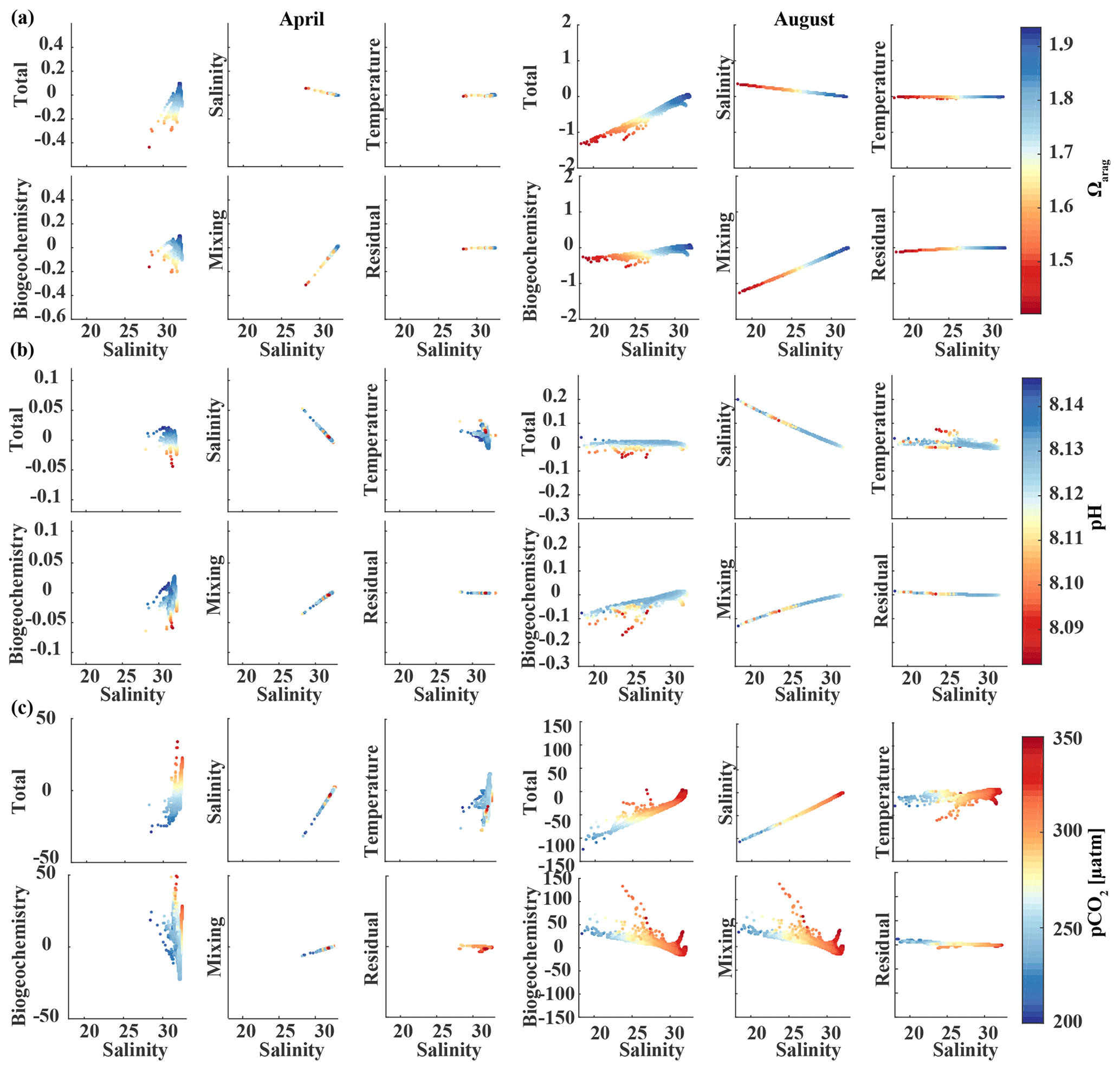
Figure 14Component distributions of the linear Taylor decomposition of surface (a) Ωarag, (b) pH, and (c) pCO2 vs. salinity in April (left) and August (right). Following Rheuban et al. (2019), the components are total perturbation from the oceanic end-member (salinity > 32); perturbations due to salinity, temperature, biogeochemistry, and freshwater mixing; and an estimated residual term.
Here, we introduced a new regional biogeochemical model, GOA-COBALT, and evaluated the model's skill in simulating seasonal and interannual inorganic carbon patterns. Our model setup is unique because it includes a moderately high-resolution, three-dimensional regional ocean circulation model, a complex ecosystem model with an ocean carbon cycle, a high-resolution terrestrial hydrological model, and it is forced with reanalysis products to simulate interannual variability and long-term changes over the past 30+ years. In addition, we used available TA and DIC observations to parameterize seasonal concentrations of DIC and TA in the freshwater forcing.
Comparison with a limited amount of in situ inorganic carbon observations showed that the model is able to reproduce the general hydrographic and inorganic carbon patterns along the Seward Line in spring and fall. GOA-COBALT was particularly successful in reproducing the depth of the aragonite saturation horizon, showing oversaturated conditions across large parts of the shelf in May and undersaturation across the shelf in September (Figs. 4, 5). GOA-COBALT generally overestimates peak Chl-α concentrations throughout spring and summer (Fig. 3). However, the results of the inorganic carbon data–model analysis suggest that DIC is not drawn down enough by spring biological production (Fig. 4). This contradiction may be due to an underestimation of the modeled C : Chl-α ratios, which are dependent on light and nutrient limitation (Geider et al., 1997; Stock et al., 2014). Modeled C : Chl-α of large and small phytoplankton on the shelf are <30 and <40 g g−1, respectively. Measurements of C : Chl-α of small phytoplankton in the GOA suggest a median C : Chl-α of 41 g g−1 during intense and early blooms and 76 g g−1 under low-Chl-α conditions (Strom et al., 2016). Equivalent data for large phytoplankton do not exist.
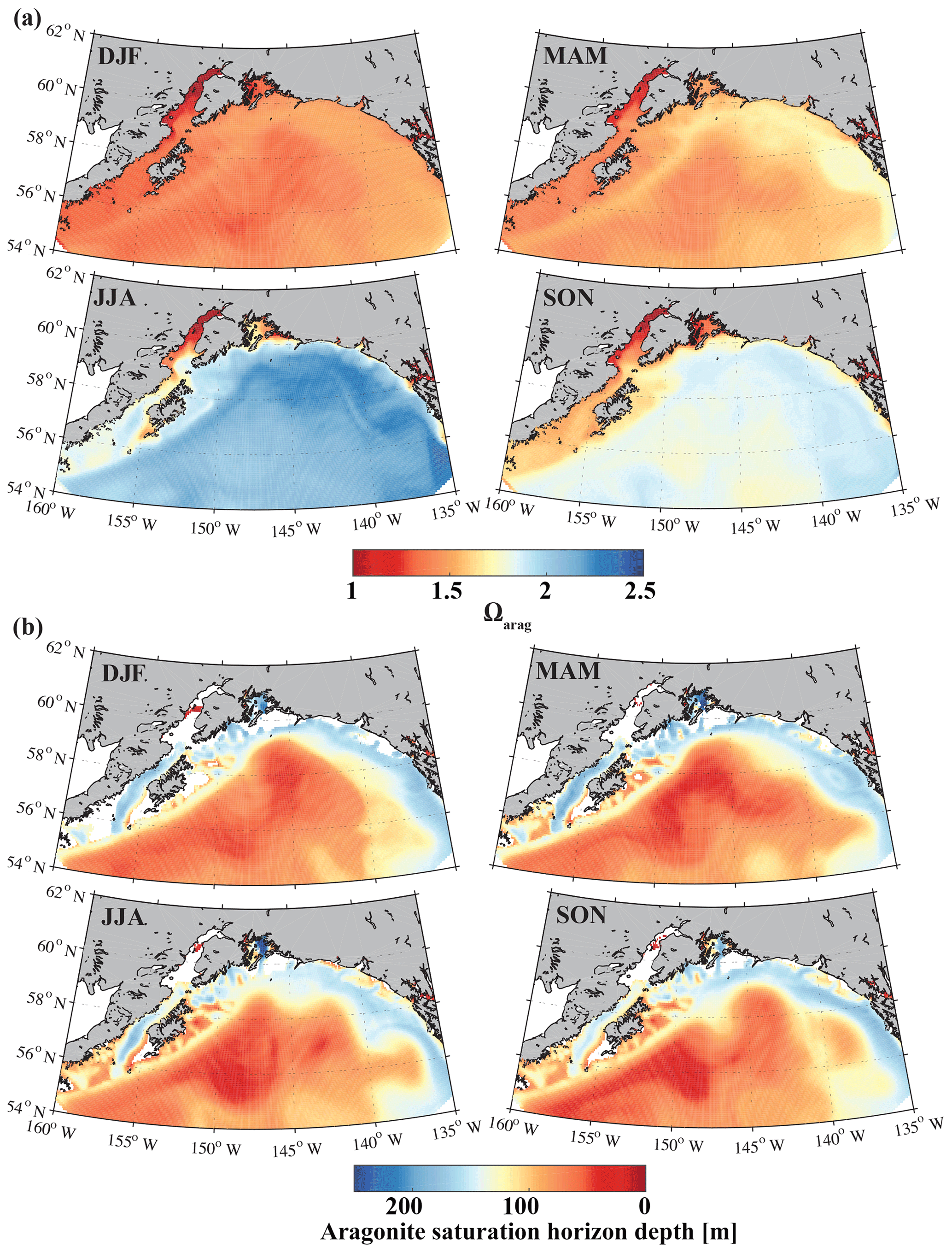
Figure 15Climatological mean of (a) the surface aragonite saturation state (Ωarag) and (b) the aragonite saturation horizon (m) for December, January, and February (DJF); March, April, and May (MAM); June, July, and August (JJA); and September, October, and November (SON).
GOA-COBALT is more successful in reproducing surface inorganic carbon patterns in September, when freshwater is the dominant driver of the system. However, the limited amount of inorganic carbon observations that cover one transect in May and September and include a few newer nearshore time series are not sufficient to properly evaluate the model. More observations are needed to test the model's skill in areas other than the Seward Line and during other times of the year. While some of the year-to-year differences seen in Figs. 7 and 8 may be a result of aliasing the spatial and temporal variability that exists during the cruises, the most prominent anomalies reproduced by the model have been described in the past. For example, as a result of anomalies in coastal runoff, winter cooling, stratification, and winds, sea surface temperature was 1.5 ∘C colder in spring 2006, 2007, and 2008 than the average spring temperatures, and they were the lowest spring temperatures since early 1970 (Janout et al., 2010). In contrast, as a result of warm air temperatures, GOA sea surface temperatures in 2010 were anomalously high (Danielson et al., 2019).
The observed seasonal relationships between Ωarag, pH, and pCO2 in freshwater-influenced coastal waters off Alaska are different from those found in other regions, such as the open ocean (Fig. 13). Similarly to the in situ observations of Evans et al. (2014) near a tidewater glacier in Prince William Sound, our freshwater inorganic carbon analysis showed that low Ωarag values are not always accompanied by low pH and high pCO2 values in this glacially influenced environment. This decoupling of the three inorganic carbon parameters is driven by the additive effects of salinity and mixing with low TA and DIC end-members. The fact that freshwater-induced low surface pCO2 caused enhanced CO2 uptake in coastal areas, as speculated by Evans et al. (2014), could not be confirmed here and will require additional investigation.
The strong influence of freshwater on the inorganic carbon system emphasizes the importance of choosing the right DIC and TA concentrations in freshwater in order to correctly model the inorganic carbon dynamics in this area. However, there is a lack of biogeochemical data that describe the composition of different freshwater sources on seasonal timescales. The biogeochemical composition of freshwater is influenced by its exposure to basal rock and, therefore, by the pathways and duration it takes and the processes it undergoes until it is introduced to the ocean (Lacroix et al., 2020). Current sources of freshwater in the GOA are tidewater glaciers, proglacial streams, and non-glacial streams, each exposing the water to basal rock, soils, and the atmosphere differently. As rapid deglaciation continues in this region (Arendt et al., 2002; Larsen et al., 2007; O'Neel et al., 2005), not only will the amount of freshwater discharge increase (Beamer et al., 2017), but most of the glaciers surrounding the GOA will recede away from the ocean and into higher elevations (Huss and Hock, 2015), resulting in a change in the biogeochemical composition of freshwater. This and previous studies have shown that freshwater discharge is the largest driver of the nearshore inorganic carbon dynamics in summer and fall, and this is known to exacerbate the effects of ocean acidification (Evans et al., 2014; Siedlecki et al., 2017; Pilcher et al., 2018). Therefore, understanding the composition of freshwater sources is particularly important for the study of long-term trends of ocean acidification in the GOA-LME. As a first best approach, we used seasonal observations of DIC and TA from Kenai River (proglacial river) and applied them to every freshwater point source across the domain; however, this approach likely masks out large differences in the biogeochemical composition of freshwater input that could have implications for the coastal inorganic carbon system.
Precipitation is only counted as negative salt flux and does not change the volume or dilute any other parameters in this current GOA-COBALT model version. While the decrease in salinity increases Ωarag and pH and decreases pCO2 (Fig. 14), our model does not account for the diluting effect of low-TA and low-DIC rainwater. Annual mean riverine input into our model domain is 1.5 times higher than annual mean precipitation across the first 100 km along the coast and up to 7 times higher across the first 10 km along the coast. Model cells in the vicinity of large rivers, such as the Copper River, receive up to 3 orders of magnitude more freshwater from rivers than from precipitation. Furthermore, the modeled surface salinity pattern closely reflects the influence of riverine input (Fig. 13), whereas the precipitation pattern is not mirrored (not shown). Thus, the diluting effect of precipitation on TA and DIC seems to be negligible compared with the large volumes of water coming in from the thousands of streams and rivers along the coast. However, this hypothesis still needs to be tested, especially because rain may increase in the future as a result of climate change (McAfee et al., 2014).
The only other regional biogeochemical model with an oceanic carbon cycle (Siedlecki et al., 2017; Pilcher et al., 2018) used the monthly riverine input time series from Royer (1982) and applied it equally to the top cell along the coast, masking out the large spatial and interannual variability of freshwater input along the GOA coast. Furthermore, Siedlecki et al. (2017) simulated the year 2009, with only 1 year of spin-up and with DIC and TA boundary conditions based on salinity relationships. Their static freshwater TA concentration to represent a tidewater glacier was 650 µmol kg−1, while freshwater runoff did not affect coastal DIC at all. In comparison, our GOA-COBALT model and the model from Siedlecki et al. (2017) both simulate the lowest surface Ωarag in winter and the highest surface Ωarag in summer (Fig. 15). Similarly, the aragonite saturation horizon is shallowest in summer and fall in both models. In our model, the aragonite saturation horizon is shallower throughout the year, causing aragonite undersaturation across wider areas on the shelf. A thorough model intercomparison study would need to be carried out to understand how the new features of our model setup have affected and potentially improved the modeling results over Siedlecki et al. (2017) and Pilcher et al. (2018).
Our simulation results give new and important insights for months of the year that lack in situ inorganic carbon observations. For example, the majority of the near-bottom water along the Seward Line is seasonally undersaturated with respect to aragonite between June and January. Such long and reoccurring aragonite undersaturation events may be harmful to some organisms. Furthermore, between January and March, conditions are unfavorable for pteropods across the entire water column with an aragonite saturation state <1.5 (Bednaršek et al., 2019). This study also made it apparent that more observations across the shelf and different times of the year are needed in order to improve the model and evaluate its skill in areas other than near the Seward Line.
Future work will focus on the progression of ocean acidification and climate change and impacts on the inorganic carbon chemistry. We also anticipate this simulation to be a useful tool for the study of the duration and intensity of extreme events and climate–ocean teleconnections. With increased confidence in the model, another logical next step would be to guide the future expansion, diversification, and optimization of ocean acidification observing systems in the GOA-LME through the northern Gulf of Alaska Long Term Ecological Research (https://nga.lternet.edu/, last access: 21 July 2020), Alaska Ocean Acidification Network (https://aoos.org/alaska-ocean-acidification-network/, last access: 21 July 2020) and the NOAA Ocean Acidification Program (https://oceanacidification.noaa.gov/, last access: 21 July 2020).
The code and forcing files are available on zenodo.org from the following DOIs: https://doi.org/10.5281/zenodo.3647663 (Hedstrom, 2020), https://doi.org/10.5281/zenodo.3661518 (Hedstrom et al., 2020a), and https://doi.org/10.5281/zenodo.3647609 (Hedstrom et al., 2020b). The model output is publicly available (https://doi.org/10.24431/rw1k43t, Hauri et al., 2020) and can be visualized with a user-friendly web interface. This is a product of our collaboration with Axiom Data Science.
KH, CH, SD, CAS, and CS developed and tuned the model system for the Gulf of Alaska. CH and BI prepared the model output. CH, CS, BI, and SCD analyzed the model output. RD ported the COBALT code into the Regional Ocean Model System. All authors commented on the paper.
The authors declare that they have no conflict of interest.
The model development and model output analysis was funded by the National Science Foundation (NSF; grant no. OCE-1459834). Claudine Hauri, Katherine Hedstrom, Seth Danielson, Scott Doney, and Cristina Schultz also acknowledge funding from the NSF (grant no. PLR-1602654). Claudine Hauri is grateful for support from National Science Foundation (grant nos. OCE-1656070 and OIA-1757348). The Seward Line and Northern Gulf of Alaska Long Term Ecological Research programs provided observations for the model evaluation. Model simulations were performed using the Chinook supercomputer at the University of Alaska Fairbanks. The authors would like to thank Eran Hood (UAS) and Sarah Stackpoole (USGS) for sharing their riverine nutrient, oxygen, and inorganic carbon chemistry data.
This research has been supported by the National Science Foundation, Division of Ocean Sciences (grant nos. 1459834 and 1656070); the National Science Foundation, Office of Polar Programs (grant no. 1602654); and the National Science Foundation, Office of Integrative Activities (grant no. 1757348).
This paper was edited by Peter Landschützer and reviewed by three anonymous referees.
Adcroft, A., Anderson, W., Balaji, V., Blanton, C., Bushuk, M., Dufour, C. O., Dunne, J. P., Griffies, S. M., Hallberg, R., Harrison, M. J., Held, I. M., Jansen, M. F., John, J. G., Krasting, J. P., Langenhorst, A. R., Legg, S., Liang, Z., McHugh, C., Radhakrishnan, A., Reichl, B. G., Rosati, T., Samuels, B. L., Shao, A., Stouffer, R., Winton, M., Wittenberg, A. T., Xiang, B., Zadeh, N., and Zhang, R.: The GFDL Global Ocean and Sea Ice Model OM4.0: Model Description and Simulation Features, J. Adv. Model. Earth Sy., pp. 3167–3211, https://doi.org/10.1029/2019MS001726, 2019. a
Aguilar-Islas, A. M., Séguret, M. J., Rember, R., Buck, K. N., Proctor, P., Mordy, C. W., and Kachel, N. B.: Temporal variability of reactive iron over the Gulf of Alaska shelf, Deep-Sea Rese. Pt. II, 132, 90–106, https://doi.org/10.1016/j.dsr2.2015.05.004, 2015. a, b, c, d, e, f
Arendt, A. A., Echelmeyer, K. A., Harrison, W. D., Lingle, C. S., and Valentine, V. B.: Rapid wastage of Alaska glaciers and their contribution to rising sea level, Science, 297, 382–386, https://doi.org/10.1126/science.1072497, 2002. a, b
Beamer, J. P., Hill, D. F., Arendt, A., and Liston, G. E.: High-resolution modeling of coastal freshwater discharge and glacier mass balance in the Gulf of Alaska watershed, Water Resour. Res., 52, 3888–3909, https://doi.org/10.1002/2015WR018457, 2016. a, b, c
Beamer, J. P., Hill, D. F., McGrath, D., Arendt, A., and Kienholz, C.: Hydrologic impacts of changes in climate and glacier extent in the Gulf of Alaska watershed, Water Resour. Res., 53, 7502–7520, https://doi.org/10.1002/2016WR020033, 2017. a
Bednaršek, N., Feely, R. A., Howes, E. L., Hunt, B. P. V., Kessouri, F., León, P., Lischka, S., Maas, A. E., McLaughlin, K., Nezlin, N. P., Sutula, M., and Weisberg, S. B.: Systematic review and meta-analysis toward synthesis of thresholds of ocean acidification impacts on calcifying pteropods and interactions with warming, Front. Mar. Sci., 6, 1–16, https://doi.org/10.3389/fmars.2019.00227, 2019. a
Byrne, R. H., Mecking, S., Feely, R. A., and Liu, X.: Direct observations of basin-wide acidification of the North Pacific Ocean, Geophys. Res. Lett., 37, 1–5, https://doi.org/10.1029/2009GL040999, 2010. a
Carter, B. R., Feely, R. A., Mecking, S., Cross, J. N., Macdonald, A. M., Siedlecki, S. A., Talley, L. D., Sabine, C. L., Millero, F. J., Swift, J. H., Dickson, A. G., and Rodgers, K. B.: Two decades of Pacific anthropogenic carbon storage and ocean acidification along Global Ocean Ship-based Hydrographic Investigations Program sections P16 and P02, Global Biogeochem. Cy., 31, 306–327, https://doi.org/10.1002/2016GB005485, 2017. a, b, c
Carton, J. A., Chepurin, G. A., Chen, L., Carton, J. A., Chepurin, G. A., and Chen, L.: SODA3: A new ocean climate reanalysis, J. Climate, 31, 6967–6983, https://doi.org/10.1175/JCLI-D-18-0149.1, 2018. a
Coyle, K. O., Cheng, W., Hinckley, S. L., Lessard, E. J., Whitledge, T., Hermann, A. J., and Hedstrom, K.: Model and field observations of effects of circulation on the timing and magnitude of nitrate utilization and production on the northern Gulf of Alaska shelf, Prog. Oceanogr., 103, 16–41, https://doi.org/10.1016/j.pocean.2012.03.002, 2012. a, b, c
Crusius, J., Schroth, A. W., Resing, J. A., Cullen, J., and Campbell, R. W.: Seasonal and spatial variability in northern Gulf of Alaska surface-water iron concentrations driven by shelf sediment resuspension, glacial meltwater, a Yakutat eddy, and dust, Global Biogeochem. Cy., 31, 942–960, https://doi.org/10.1002/2016GB005493, 2017. a, b
Danielson, S., Hennon, T., Monson, D., Suryan, R., Campbell, R., Baird, S., Holderied, K., and Weingartner, T.: Chapter 1 A study of marine temperature variations in the northern Gulf of Alaska across years of marine heatwaves and cold spells, in: The Pacific Marine Heatwave: Monitoring During a Major Perturbation, edited by: Suryan, M. R., Lindeberg, M. R., and Aderhold, D. R., Tech. rep., Exxon Valdez Oil Spill Trustee Council, Anchorage, AK, 2019. a
Danielson, S., Hill, D., Hedstrom, K., Beamer, J., and Curchitser, E.: Coupled terrestrial hydrological and ocean circulation modeling across the Gulf of Alaska coastal interface, J. Geophys. Res.-Oceans, https://doi.org/10.1029/2019JC015724, online first, 2020. a, b, c, d
Danielson, S. L., Hedstrom, K. S., and Curchitser, E.: Cook Inlet Circulation Model Calculations, Tech. rep., University of Alaska Fairbanks, Fairbanks, AK, 2016. a
Dickson, A.: The boron/chlorinity ratio of deep-sea water from the Pacific Ocean, Deep-Sea Res., 21, 161–162, https://doi.org/10.1016/0011-7471(74)90074-6, 1974. a
Dickson, A.: Thermodynamics of the dissociation of boric acid in synthetic seawater from 273.15 to 318.15 K, Deep-Sea Res., 37, 755–766, https://doi.org/10.1016/0198-0149(90)90004-F, 1990. a
Dobbins, E. L., Hermann, A. J., Stabeno, P., Bond, N. A., and Steed, R. C.: Modeled transport of freshwater from a line-source in the coastal Gulf of Alaska, Deep-Sea Res. Pt. II, 56, 2409–2426, https://doi.org/10.1016/j.dsr2.2009.02.004, 2009. a
Evans, W. and Mathis, J. T.: The Gulf of Alaska coastal ocean as an atmospheric CO2 sink, Cont. Shelf Res., 65, 52–63, https://doi.org/10.1016/j.csr.2013.06.013, 2013. a, b
Evans, W., Mathis, J. T., Winsor, P., Statscewich, H., and Whitledge, T. E.: A regression modeling approach for studying carbonate system variability in the northern Gulf of Alaska, J. Geophys. Res.-Oceans, 118, 476–489, https://doi.org/10.1029/2012JC008246, 2013. a, b, c, d
Evans, W., Mathis, J. T., and Cross, J. N.: Calcium carbonate corrosivity in an Alaskan inland sea, Biogeosciences, 11, 365–379, https://doi.org/10.5194/bg-11-365-2014, 2014. a, b, c, d, e, f, g, h
Evans, W., Mathis, J. T., Ramsay, J., and Hetrick, J.: On the Frontline: Tracking Ocean Acidification in an Alaskan Shellfish Hatchery, Plos One, 10, e0130384, https://doi.org/10.1371/journal.pone.0130384, 2015. a
Fabry, V., McClintock, J., Mathis, J., and Grebmeier, J.: Ocean Acidification at High Latitudes: The Bellwether, Oceanography, 22, 160–171, https://doi.org/10.5670/oceanog.2009.105, 2009. a, b, c
Feely, R. A. and Chen, A.: The effect of excess CO2 on the calculated calcite and aragonite satruration horizons in the northeast pacific, Geophys. Res. Lett., 9, 1294–1297, https://doi.org/10.1029/GL009i011p01294, 1982. a
Feely, R. A., Byrne, R. H., Acker, J. G., Betzer, P. R., Chen, C.-T. A., Gendron, J. F., and Lamb, M. F.: Winter–summer variations of calcite and Aragonite saturation in the Northeast Pacific, Mar. Chem., 25, 227–241, https://doi.org/10.1016/0304-4203(88)90052-7, 1988. a
Fellman, J. B., Hood, E., Dryer, W., and Pyare, S.: Stream Physical Characteristics Impact Habitat Quality for Pacific Salmon in Two Temperate Coastal Watersheds, Plos One, 10, e0132652, https://doi.org/10.1371/journal.pone.0132652, 2015. a
Fiechter, J. and Moore, A. M.: Interannual spring bloom variability and Ekman pumping in the coastal Gulf of Alaska, J. Geophys. Res., 114, C06004, https://doi.org/10.1029/2008JC005140, 2009. a
Fiechter, J., Moore, A. M., Edwards, C. A., Bruland, K. W., Di Lorenzo, E., Lewis, C. V., Powell, T. M., Curchitser, E. N., and Hedstrom, K.: Modeling iron limitation of primary production in the coastal Gulf of Alaska, Deep-Sea Res. Pt. II, 56, 2503–2519, https://doi.org/10.1016/j.dsr2.2009.02.010, 2009. a
Franco, A. C., Gruber, N., Frölicher, T. L., and Kropuenske Artman, L.: Contrasting Impact of Future CO2 Emission Scenarios on the Extent of CaCO3 Mineral Undersaturation in the Humboldt Current System, J. Geophys. Res.-Oceans, 123, 2018–2036, https://doi.org/10.1002/2018JC013857, 2018. a
Garcia, H. E., Locarnini, R. A., Boyer, T. P., Antonov, J. I., Baranova, O. K., Zweng, M. M., Reagan, J. R., and Johnson, D. R.: World Ocean Atlas 2013, Volume 4: Dissolved Inorganic Nutrients (phosphate, nitrate, silicate), NOAA Atlas NESDIS 76, 27 pp., https://doi.org/10.1182/blood-2011-06-357442, 2013. a
Geider, R. J., MacIntyre, H. L., and Kana, T. M.: Dynamic model of phytoplankton growth and acclimation: Responses of the balanced growth rate and the chlorophyll a:carbon ratio to light, nutrient-limitation and temperature, Mar. Ecol.-Prog. Ser., 148, 187–200, https://doi.org/10.3354/meps148187, 1997. a
Gruber, N., Hauri, C., Lachkar, Z., Loher, D., Frölicher, T. L., and Plattner, G.-K.: Rapid Progression of Ocean Acidification in the California Current System, Science, 220, 220–223, https://doi.org/10.1126/science.1216773, 2012. a
Hare, S. R. and Mantua, N. J.: Empirical evidence for North Pacific regime shifts in 1977 and 1989, Prog. Oceanogr. 47, 103–145, https://doi.org/10.1016/S0079-6611(00)00033-1, 2000. a
Hauri, C., Gruber, N., Vogt, M., Doney, S. C., Feely, R. A., Lachkar, Z., Leinweber, A., McDonnell, A. M. P., Munnich, M., and Plattner, G.-K.: Spatiotemporal variability and long-term trends of ocean acidification in the California Current System, Biogeosciences, 10, 193–216, https://doi.org/10.5194/bg-10-193-2013, 2013. a, b
Hauri, C., Hedstrom, K., and Danielson, S.: Gulf of Alaska ROMS-COBALT Hindcast Simulation 1980–2013, Research Workspace, version: 10.24431_rw1k43t_20203421026, https://doi.org/10.24431/rw1k43t, 2020. a
Hedstrom, K.: kshedstrom/Apps_master: For use with v3.8_cobalt of ROMS (Version v1.0), Zenodo, https://doi.org/10.5281/zenodo.3647663, 2020. a
Hedstrom, K., Mack, S., Hadfield, M., and Hetland, R.: kshedstrom/roms: Master branch with COBALT mid 2019 (Version v3.8_cobalt), Zenodo, https://doi.org/10.5281/zenodo.3661518, 2020a. a
Hedstrom, K., Mack, S., Hadfield, M., and Hetland, R.: kshedstrom/roms: Master branch with COBALT early 2020 (Version v3.9_cobalt), Zenodo, https://doi.org/10.5281/zenodo.3647609, 2020b. a
Hill, D. F., Bruhis, N., Calos, S. E., Arendt, A., and Beamer, J.: Spatial and temporal variability of freshwater discharge into the Gulf of Alaska, J. Geophys. Res.-Oceans, 120, 634–646, https://doi.org/10.1002/2014JC010395, 2015. a, b
Hood, E. and Berner, L.: Effects of changing glacial coverage on the physical and biogeochemical properties of coastal streams in southeastern Alaska, J. Geophys. Res.-Biogeo., 114, 1–10, https://doi.org/10.1029/2009JG000971, 2009. a
Hood, E., Battin, T. J., Fellman, J., O'Neel, S., Spencer, R. G. M., O'Neel, S., and Spencer, R. G. M.: Storage and release of organic carbon from glaciers and ice sheets, Nat. Geosci., 8, 1–6, https://doi.org/10.1038/ngeo2331, 2015. a
Huss, M. and Hock, R.: A new model for global glacier change and sea-level rise, Front. Earth Sci., 3, 1–22, https://doi.org/10.3389/feart.2015.00054, 2015. a
Janout, M. A., Weingartner, T. J., Royer, T. C., and Danielson, S. L.: On the nature of winter cooling and the recent temperature shift on the northern Gulf of Alaska shelf, J. Geophys. Res., 115, C05023, https://doi.org/10.1029/2009JC005774, 2010. a, b
Lacroix, F., Ilyina, T., and Hartmann, J.: Oceanic CO2 outgassing and biological production hotspots induced by pre-industrial river loads of nutrients and carbon in a global modeling approach, Biogeosciences, 17, 55–88, https://doi.org/10.5194/bg-17-55-2020, 2020. a
Large, W. G. and Yeager, S. G.: The global climatology of an interannually varying air–sea flux data set, Clim. Dynam., 33, 341–364, https://doi.org/10.1007/s00382-008-0441-3, 2008. a
Larsen, C. F., Motyka, R. J., Arendt, A. A., Echelmeyer, K. A., and Geissler, P. E.: Glacier changes in southeast Alaska and northwest British Columbia and contribution to sea level rise, J. Geophys. Res.-Earth, 112, 1–11, https://doi.org/10.1029/2006JF000586, 2007. a, b
Lauvset, S. K., Key, R. M., Olsen, A., van Heuven, S., Velo, A., Lin, X., Schirnick, C., Kozyr, A., Tanhua, T., Hoppema, M., Jutterström, S., Steinfeldt, R., Jeansson, E., Ishii, M., Perez, F. F., Suzuki, T., and Watelet, S.: A new global interior ocean mapped climatology: the 1∘ × 1∘ GLODAP version 2, Earth Syst. Sci. Data, 8, 325–340, https://doi.org/10.5194/essd-8-325-2016, 2016. a
Lewis, E. and Wallace, D. W. R.: Program Developed for CO2 System Calculations, ORNL/CDIAC-105, Carbon Dioxide Inf. Anal. Cent., Oak Ridge Natl. Lab., Oak Ridge, Tenn., 38 pp., available at: https://salish-sea.pnnl.gov/media/ORNL-CDIAC-105.pdf (last access: July 2020), 1998. a
Li, Q. and Fox-Kemper, B.: Assessing the effects of Langmuir turbulence on the entrainment buoyancy flux in the ocean surface boundary layer, J. Phys. Oceanogr., 47, 2863–2886, https://doi.org/10.1175/JPO-D-17-0085.1, 2017. a
Lippiatt, S. M., Lohan, M. C., and Bruland, K. W.: The distribution of reactive iron in northern Gulf of Alaska coastal waters, Mar. Chem., 121, 187–199, https://doi.org/10.1016/j.marchem.2010.04.007, 2010. a, b, c, d
Liston, G. and Elder, K.: A Meteorological Distribution System for High-Resolution Terrestrial Modeling (MicroMet), J. Hydrometeorol., 7, 217–234, https://doi.org/10.1175/JHM486.1, 2006. a
Lueker, T., Dickson, A., and Keeling, C.: Ocean pCO2 calculated from dissolved inorganic carbon, alkalinity, and equations for K1 and K2: validation based on laboratory measurements of CO2 in gas and seawater at equilibrium, Mar. Chem., 70, 105–119, https://doi.org/10.1016/S0304-4203(00)00022-0, 2000. a
Manizza, M., Le Quéré, C., Watson, A. J., and Buitenhuis, E. T.: Bio-optical feedbacks among phytoplankton, upper ocean physics and sea-ice in a global model, Geophys. Res. Lett., 32, 1–4, https://doi.org/10.1029/2004GL020778, 2005. a
Martin, J. H., Gordon, R., Fitzwater, S., and Broenkow, W. W.: Vertex: phytoplankton/iron studies in the Gulf of Alaska, Deep-Sea Res. Pt. A, 36, 649–680, https://doi.org/10.1016/0198-0149(89)90144-1, 1989. a, b
Mathis, J., Cooley, S., Lucey, N., Colt, S., Ekstrom, J., Hurst, T., Hauri, C., Evans, W., Cross, J., and Feely, R.: Ocean Acidification Risk Assessment for Alaska's Fishery Sector, Prog. Oceanogr., 136, 71–91, https://doi.org/10.1016/j.pocean.2014.07.001, 2014. a
McAfee, S. A., Walsh, J., and Rupp, T. S.: Statistically downscaled projections of snow/rain partitioning for Alaska, Hydrol. Process., 28, 3930–3946, https://doi.org/10.1002/hyp.9934, 2014. a
Miller, C. A., Pocock, K., Evans, W., and Kelley, A. L.: An evaluation of the performance of Sea-Bird Scientific's SeaFET™ autonomous pH sensor: considerations for the broader oceanographic community, Ocean Sci., 14, 751–768, https://doi.org/10.5194/os-14-751-2018, 2018. a
MODIS-Aqua Ocean Color Data, NASA Goddard Space Flight Center, Ocean Ecology Laboratory: NASA Goddard Space Flight Center, Ocean Ecology Laboratory, Ocean Biology Processing Group, https://doi.org/10.5067/AQUA/MODIS_OC.2014.0 (last access: 17 August 2019), 2014. a, b
Mundy, P.: The Gulf of Alaska: biology and oceanography, University of Alaska, Alaska Sea Grant College Program, Fairbanks, AK, 2005. a
Neal, E. G., Hood, E., and Smikrud, K.: Contribution of glacier runoff to freshwater discharge into the Gulf of Alaska, Geophys. Res. Lett., 37, L06404, https://doi.org/10.1029/2010GL042385, 2010. a
O'Neel, S., Pfeffer, W. T., Krimmel, R., and Meier, M.: Evolving force balance at Columbia Glacier, Alaska, during its rapid retreat, J. Geophys. Res.-Earth, 110, 1–18, https://doi.org/10.1029/2005JF000292, 2005. a, b
Pilcher, D. J., Siedlecki, S. A., Hermann, A. J., Coyle, K. O., Mathis, J. T., and Evans, W.: Simulated impact of glacial runoff on CO2 uptake in the Gulf of Alaska, Geophys. Res. Lett., 45, 880–890, https://doi.org/10.1002/2017GL075910, 2018. a, b, c
Redfield, A. C., Ketchum, B. H., and Richards, F. A.: The Influence of Organisms on the Composition of the Sea Water, in: The Sea, Vol. 2, edited by: Hill, M. N., Interscience Publishers, New York, 26–77, 1963. a
Reisdorph, S. C. and Mathis, J. T.: The dynamic controls on carbonate mineral saturation states and ocean acidification in a glacially dominated estuary, Estuar. Coast. Shelf S., 144, 8–18, https://doi.org/10.1016/j.ecss.2014.03.018, 2014. a, b
Rheuban, J. E., Doney, S. C., McCorkle, D. C., and Jakuba, R. W.: Quantifying the effects of nutrient enrichment and freshwater mixing on coastal ocean acidification, J. Geophys. Res.-Oceans, 124, 9085–9100, https://doi.org/10.1029/2019JC015556, 2019. a, b, c, d
Royer, T. C.: Coastal fresh water discharge in the northeast Pacific, J. Goephys. Res., 87, 2017–2021, https://doi.org/10.1029/JC087iC03p02017, 1982. a, b, c
Saha, S., Moorthi, S., Pan, H. L., Wu, X., Wang, J., Nadiga, S., Tripp, P., Kistler, R., Woollen, J., Behringer, D., Liu, H., Stokes, D., Grumbine, R., Gayno, G., Wang, J., Hou, Y. T., Chuang, H. Y., Juang, H. M. H., Sela, J., Iredell, M., Treadon, R., Kleist, D., Van Delst, P., Keyser, D., Derber, J., Ek, M., Meng, J., Wei, H., Yang, R., Lord, S., Van Den Dool, H., Kumar, A., Wang, W., Long, C., Chelliah, M., Xue, Y., Huang, B., Schemm, J. K., Ebisuzaki, W., Lin, R., Xie, P., Chen, M., Zhou, S., Higgins, W., Zou, C. Z., Liu, Q., Chen, Y., Han, Y., Cucurull, L., Reynolds, R. W., Rutledge, G., and Goldberg, M.: The NCEP climate forecast system reanalysis, B. Am. Meteorol. Soc., 91, 1015–1057, https://doi.org/10.1175/2010BAMS3001.1, 2010. a
Shchepetkin, A. F. and McWilliams, J. C.: The regional oceanic modeling system (ROMS): a split-explicit, free-surface, topography-following-coordinate oceanic model, Ocean Model., 9, 347–404, https://doi.org/10.1016/j.ocemod.2004.08.002, 2005. a
Siedlecki, S. A., Pilcher, D. J., Hermann, A. J., Coyle, K., and Mathis, J.: The Importance of Freshwater to Spatial Variability of Aragonite Saturation State in the Gulf of Alaska, J. Geophys. Res.-Oceans, 122, 8482–8502, https://doi.org/10.1002/2017JC012791, 2017. a, b, c, d, e, f, g, h
Stabeno, P., Bond, N., Hermann, A., Kachel, N., Mordy, C., and Overland, J.: Meteorology and oceanography of the Northern Gulf of Alaska, Cont. Shelf Res., 24, 859–897, https://doi.org/10.1016/j.csr.2004.02.007, 2004. a
Stackpoole, S., Butman, D., Clow, D., Verdin, K., Gaglioti, B., and Striegl, R. G.: Carbon burial, transport, and emission from inland aquatic ecosystems in Alaska, USGS Professional Paper, 1826, 159–188, https://doi.org/10.3133/pp1826, 2016. a, b, c, d
Stackpoole, S. M., Butman, D., Clow, D. W., Verdin, K. L., Gaglioti, B. V., Genet, H., and Striegl, R. G.: Inland waters and their role in the carbon cycle of Alaska, Ecol. Appl., 27, 1403–1420, https://doi.org/10.1002/eap.1552, 2017. a, b, c, d
Stock, C. A., Dunne, J. P., and John, J. G.: Global-scale carbon and energy flows through the marine planktonic food web: An analysis with a coupled physical–biological model, Prog. Oceanogr., 120, 1–28, https://doi.org/10.1016/j.pocean.2013.07.001, 2014. a, b, c
Strom, S. L., Olson, M. B., Macri, E. L., and Mordy, C. W.: Cross-shelf gradients in phytoplankton community structure, nutrient utilization, and growth rate in the coastal Gulf of Alaska, Mar. Ecol.-Prog. Ser., 328, 75–92, https://doi.org/10.3354/Meps328075, 2007. a
Strom, S. L., Macri, E. L., and Fredrickson, K. A.: Light limitation of summer primary production in the coastal Gulf of Alaska: Physiological and environmental causes, Mar. Ecol.-Prog. Ser., 402, 45–57, https://doi.org/10.3354/meps08456, 2010. a, b
Strom, S. L., Fredrickson, K. A., and Bright, K. J.: Spring phytoplankton in the eastern coastal Gulf of Alaska: Photosynthesis and production during high and low bloom years, Deep-Sea Res. Pt. II, 132, 107–121, https://doi.org/10.1016/j.dsr2.2015.05.003, 2016. a
Sutton, A. J., Feely, R. A., Maenner-Jones, S., Musielwicz, S., Osborne, J., Dietrich, C., Monacci, N., Cross, J., Bott, R., and Kozyr, A.: Autonomous seawater pCO2 and pH time series from 40 surface buoys and the emergence of anthropogenic trends, Earth Syst. Sci. Data Discuss., https://doi.org/10.5194/essd-2018-77, 2018. a
Takahashi, T., Sutherland, S. C., Chipman, D. W., Goddard, J. G., Ho, C., Newberger, T., Sweeney, C., and Munro, D. R.: Climatological distributions of pH, pCO2, total CO2, alkalinity, and CaCO3 saturation in the global surface ocean, and temporal changes at selected locations, Mar. Chem., 164, 95–125, https://doi.org/10.1016/j.marchem.2014.06.004, 2014. a
Taylor, K. E.: Summarizing multiple aspects of model performance in a single diagram, J. Geophys. Res.-Atmos., 106, 7183–7192, 2001. a
Tsujino, H., Urakawa, S., Nakano, H., Small, R. J., Kim, W. M., Yeager, S. G., Danabasoglu, G., Suzuki, T., Bamber, J. L., Bentsen, M., Böning, C. W., Bozec, A., Chassignet, E. P., Curchitser, E., Boeira Dias, F., Durack, P. J., Griffies, S. M., Harada, Y., Ilicak, M., Josey, S. A., Kobayashi, C., Kobayashi, S., Komuro, Y., Large, W. G., Le Sommer, J., Marsland, S. J., Masina, S., Scheinert, M., Tomita, H., Valdivieso, M., and Yamazaki, D.: JRA-55 based surface dataset for driving ocean–sea-ice models (JRA55-do), Ocean Model., 130, 79–139, https://doi.org/10.1016/j.ocemod.2018.07.002, 2018. a
Turi, G., Lachkar, Z., Gruber, N., and Münnich, M.: Climatic modulation of recent trends in ocean acidification in the California Current System, Environ. Res. Lett., 11, 014007, https://doi.org/10.1088/1748-9326/11/1/014007, 2016. a
van Heuven, S. M. A. C., Pierrot, D., Rae, J. W. B., Lewis, E., and Wallace, D. W. R.: MATLAB Program Developed for CO2 System Calculations, ORNL/CDIAC-105b. Carbon Dioxide Information Analysis Center, Oak Ridge National Laboratory, U.S. Department of Energy, Oak Ridge, Tennessee, https://doi.org/10.3334/CDIAC/otg.CO2SYS_MATLAB_v1.1, 2011. a
Van Oostende, N., Dussin, R., Stock, C. A., Barton, A. D., Curchitser, E., Dunne, J. P., and Ward, B. B.: Simulating the ocean's chlorophyll dynamic range from coastal upwelling to oligotrophy, Prog. Oceanogr., 168, 232–247, https://doi.org/10.1016/j.pocean.2018.10.009, 2018. a, b, c
Wang, J., Jin, M., and Musgrave, D. L.: A hydrological digital elevation model for freshwater discharge into the Gulf of Alaska, J. Geophys. Res., 109, 1–15, https://doi.org/10.1029/2002JC001430, 2004. a
Weingartner, T. J., Danielson, S. L., and Royer, T. C.: Freshwater variability and predictability in the Alaska Coastal Current, Deep-Sea Res. Pt. II, 52, 169–191, https://doi.org/10.1016/j.dsr2.2004.09.030, 2005. a, b
Whitney, F. A. and Freeland, H. J.: Variability in upper-ocean water properties in the NE Pacific Ocean, Deep-Sea Res. Pt. II, 46, 2351–2370, https://doi.org/10.1016/S0967-0645(99)00067-3, 1999. a
Wu, J., Aguilar-Islas, A., Rember, R., Weingartner, T., Danielson, S., and Whitledge, T.: Size-fractionated iron distribution on the northern Gulf of Alaska, Geophys. Res. Lett., 36, L11606, https://doi.org/10.1029/2009GL038304, 2009. a, b
Xiu, P. and Chai, F.: Connections between physical, optical and biogeochemical processes in the Pacific Ocean, Prog. Oceanogr., 122, 30–53, https://doi.org/10.1016/j.pocean.2013.11.008, 2014. a, b
Xiu, P., Chai, F., Xue, H., Shi, L., and Chao, Y.: Modeling the mesoscale eddy field in the Gulf of Alaska, Deep-Sea Res. Pt. I, 63, 102–117, https://doi.org/10.1016/j.dsr.2012.01.006, 2012. a
- Abstract
- Introduction
- Methods
- Model evaluation
- Seasonal inorganic carbon variability along the Seward Line
- Influence of glacial freshwater on surface Ωarag, pH, and pCO2
- Summary and conclusions
- Code and data availability
- Author contributions
- Competing interests
- Acknowledgements
- Financial support
- Review statement
- References