the Creative Commons Attribution 4.0 License.
the Creative Commons Attribution 4.0 License.
 | 27 Aug 2020
Seasonal dynamics of the COS and CO2 exchange of a managed temperate grassland
Felix M. Spielmann
Albin Hammerle
Florian Kitz
Katharina Gerdel
Georg Wohlfahrt
Gross primary productivity (GPP), the CO2 uptake by means of photosynthesis, cannot be measured directly on the ecosystem scale but has to be inferred from proxies or models. One newly emerged proxy is the trace gas carbonyl sulfide (COS). COS diffuses into plant leaves in a fashion very similar to CO2 but is generally not emitted by plants. Laboratory studies on leaf level gas exchange have shown promising correlations between the leaf relative uptake (LRU) of COS to CO2 under controlled conditions. However, in situ measurements including daily to seasonal environmental changes are required to test the applicability of COS as a tracer for GPP at larger temporal scales. To this end, we conducted concurrent ecosystem-scale CO2 and COS flux measurements above an agriculturally managed temperate mountain grassland. We also determined the magnitude and variability of the soil COS exchange, which can affect the LRU on an ecosystem level. The cutting and removal of the grass at the site had a major influence on the soil flux as well as the total exchange of COS. The grassland acted as a major sink for CO2 and COS during periods of high leaf area. The sink strength decreased after the cuts, and the grassland turned into a net source for CO2 and COS on an ecosystem level. The soil acted as a small sink for COS when the canopy was undisturbed but also turned into a source after the cuts, which we linked to higher incident radiation hitting the soil surface. However, the soil contribution was not large enough to explain the COS emission on an ecosystem level, hinting at an unknown COS source possibly related to dead plant matter degradation. Over the course of the season, we observed a concurrent decrease in CO2 and COS uptake on an ecosystem level. With the exception of the short periods after the cuts, the LRU under high-light conditions was rather stable and indicated a high correlation between the COS flux and GPP across the growing season.
- Article
(3745 KB) - Full-text XML
-
Supplement
(1848 KB) - BibTeX
- EndNote


Carbonyl sulfide (COS) is the most abundant sulfur-containing gas in the atmosphere, with tropospheric mole fractions of ∼500 ppt. Within the atmosphere, COS acts as a greenhouse gas with a direct radiative forcing efficiency 724 times higher than CO2 (Brühl et al., 2012). After reaching the stratosphere, it reacts to sulfur aerosols via oxidation and photolysis, hence contributing to the backscattering of solar radiation and having a cooling effect on Earth's atmosphere (Krysztofiak et al., 2015; Whelan et al., 2018). The intraseasonal atmospheric COS mole fraction follows the pattern of CO2 as terrestrial vegetation acts as the largest known sink for both species (Montzka et al., 2007; Whelan et al., 2018; Le Quéré et al., 2018). However, the relative decrease in ambient mole fraction during summer of the Northern Hemisphere is 6 times stronger for COS than for CO2 (Montzka et al., 2007) as COS is generally not emitted by plants like CO2, which is released in respiration processes.
The uptake of COS by plants is mostly mediated by the enzyme carbonic anhydrase (CA) but also photolytic enzymes like Ribulose-1,5-bisphosphate-carboxylase/-oxygenase (Rubisco; Lorimer and Pierce, 1989). This in turn means that COS and CO2 share a similar pathway into leaves through the boundary layer, the stomata and the cytosol, up to their reaction sites. Compared to CO2, COS is processed in a one-way reaction to H2S and CO2 (Protoschill-Krebs and Kesselmeier, 1992; Notni et al., 2007) and therefore not released by plants, with the exception of severely stressed plants (Bloem et al., 2012; Gimeno et al., 2017). That makes COS an interesting tracer for estimating the stomatal conductance and the gross uptake of CO2, referred to as gross primary production (GPP), on an ecosystem level (Asaf et al., 2013; Kooijmans et al., 2017, 2019). However, to estimate GPP using COS, the leaf relative uptake (LRU) of COS to GPP deposition velocities must be known beforehand (see Eq. 1) so that GPP can be estimated on the basis of the COS flux.
FCOS is the COS leaf flux (pmol m−2 s−1), is the gross CO2 uptake on the leaf level (µmol m−2 s−1), and χCOS and are the ambient COS and CO2 mole fractions in parts per trillion and parts per million, respectively. Leaf level studies for C3 plants have estimated the LRU to be around 1.7, with a 95 % confidence interval between 0.7 and 6.2 (Whelan et al., 2018; Seibt et al., 2010; Sandoval-Soto et al., 2005). The large spread of the LRU most likely originates from differences between plant species, for example, leaf structure and plant metabolism (Wohlfahrt et al., 2012; Seibt et al., 2010), which questions the applicability of the concept of LRU in real-world ecosystems under naturally varying environmental conditions. It is also known that the LRU is just stable under high-light conditions since the uptake of CO2 by means of photosynthesis is a light-driven process, while CA is able to process COS independently of light conditions (Maseyk et al., 2014; Yang et al., 2018; Stimler et al., 2011). Any model of LRU should therefore reflect diurnal changes in light conditions. Kooijmans et al. (2019) recently discovered that the vapor pressure deficit (VPD) appears to have a stronger control on FCOS than on in an evergreen needle forest. If generally true, this would add further variability to the LRU and complicate the application of COS to estimate GPP. Besides interspecific differences in LRU, the question remains unanswered whether the LRU is also susceptible to seasonal changes in ecosystems, for example changes in species composition or phenology, which would further complicate the application of COS in carbon cycle research. Maseyk et al. (2014) observed COS emissions on the ecosystem scale over a winter wheat field going into senescence, indicating that potentially strong sources of COS could distort LRU.
Since CA and other enzymes known to emit or take up COS are also present in microorganisms (Ogawa et al., 2013; Seefeldt et al., 1995; Ensign, 1995; Smeulders et al., 2013; Whelan et al., 2018), recent studies have also quantified the contribution of soils to the COS ecosystem flux (Kooijmans et al., 2017; Spielmann et al., 2019; Maseyk et al., 2014). COS soil fluxes could modify the LRU on an ecosystem level and hence infer GPP if they are substantial compared to COS canopy fluxes. Similar to the ecosystem fluxes, the soil fluxes could be prone not only to diurnal but also seasonal changes, depending on the substrate availability, environmental conditions (e.g., soil temperature and moisture; Liu et al., 2010), substrate quality and quantity, and changes in the composition of the microbial communities (Kitz et al., 2019; Meredith et al., 2019). Recent studies have also linked COS soil emissions to abiotic processes dependent on light and/or temperature (Whelan and Rhew, 2015; Kitz et al., 2019; Meredith et al., 2018).
The goal of our study was to provide new insights into the seasonal variability of COS fluxes on an ecosystem, soil and canopy level. To this end, we conducted a 6-month campaign on a managed temperate mountain grassland, measuring ecosystem as well as soil COS fluxes. Since the grassland was cut four times during the campaign, we were able to observe multiple growing cycles and investigate the diel and seasonal changes in the COS fluxes and the LRU in this highly dynamic ecosystem. We hypothesize that (H1) the grassland, given its large CO2 uptake capacity (Wohlfahrt et al. 2008), is a major sink for COS and that the sink strength decreases over the course of the season; (H2) the drying of the cut grass leads to a release of COS; (H3) the LRU will change after the cuts due to stressed plants and drying plant parts in the field but is otherwise stable; and (H4) the cuts turn the soil into a COS source due to the larger amount of light reaching the soil surface (Kitz et al., 2017), but once a reasonably high leaf area index (LAI) has developed, COS is taken up by soil.
2.1 Study site and period
The study was conducted at an intensively managed mountain grassland in the municipal territory of Neustift (Austria) in the Stubai Valley (FLUXNET ID: AT-Neu). The grassland is situated at an elevation of 970 m a.s.l. in the middle of the flat valley bottom. The soil was classified as Fluvisol with an estimated depth of 1 m and the majority of roots located within the first 10 cm. Measurements were conducted between 1 June 2015 and 31 October 2015 (183 d). The vegetation was described as Pastinaco-Arrhenatheretum and consisted mainly of Dactylis glomerata, Festuca pratensis, Alopecurus pratensis, Trisetum flavescens, Ranunculus acris, Taraxacum officinale, Trifolium repens, Trifolium pratense and Carum carvi (Kitz et al., 2017). During the campaign, the grassland was cut four times (2 June, 7 July, 21 August and 1 October 2015) and the biomass left to dry on the field for up to 1 d before being removed as silage. Each year, the field site was fertilized with solid manure and cattle slurry (Hörtnagl et al., 2018) at the end of the season (7 October 2015).
2.2 Leaf area index
The LAI was estimated from assessments of the average canopy height, which were related to destructive LAI measurements, using the following sigmoid function:
where DOY is the day of the year, and a1, a2, b1 and b2 are factors that were optimized for each growing period, for example before the first cut, between cuts and after the fourth cut (Wohlfahrt et al., 2008). Additionally, biomass samples were taken on 15 occasions to assist with the LAI calculation.
2.3 Mole fraction measurements
The CO2 () and COS (χCOS) mole fractions were measured using a Quantum Cascade Laser (QCL) Mini Monitor (Aerodyne Research, Billerica, MA, USA) at a wave number of ca. 2056 cm−1 and at a frequency of 10 Hz. To minimize the effect of air temperature (Tair) changes on the instrument, we placed it in an insulated box, which in turn was located in a climate-controlled instrument hut (30 ∘C). The cooling of the laser was achieved by a chiller (ThermoCube 400, Solid State Cooling Systems, Wappinger Falls, NY, USA).
We used .25 in. Teflon™ tubing, stainless-steel fittings (SWAGELOK, Solon, OH, USA, and FITOK, Offenbach, HE, Germany), Teflon™ filters (Savilex, Eden Prairie, MN, USA) and COS-inert valves (Parker-Hannafin, Cleveland, OH, USA) to ensure that only materials known not to interact with COS were used for the measurement and calibration airflow. Since the data of the QCL and the sonic anemometer were saved on two separate PCs, a network time protocol software (NTP, Meinberg, Germany) was used to keep the time on both devices synchronized. We corrected known χCOS drift issues of the QCL (Kooijmans et al., 2016) by doing half-hourly calibrations for 1 min with a gas of known χCOS. The gas cylinders (working standards) used for the calibrations were either pressurized air (UN 1002) or nitrogen (UN 1066), which were cross-compared (when working-standard cylinders were full and close to empty) to an AcuLife-treated aluminum pressurized air cylinder obtained from the National Oceanic and Atmospheric Administration (NOAA). The latter was analyzed by the central calibration laboratory of the NOAA for its χCOS using gas chromatography with mass spectrometric detection (GC-MS) on 6 April 2015. We then linearly interpolated between the offsets of the half-hourly calibrations and used the retrieved values to correct the high-frequency COS data. Due to issues with the scale gas cylinder, no absolute concentrations were available before 16 June 2015. To increase the number of available data for the first postcut period, we extrapolated the COS mole fractions to the day of the first cut. This was done on the basis of the measured CO2 mole fractions and the mean half-hourly ratio of the ambient CO2 to COS mole fractions retrieved between 16 and 18 June 2015.
2.3.1 Mole fraction measurements within the canopy
In order to investigate the χCOS within the canopy, we used a multiplexer and 8.25 in. Teflon™ tubes to measure the χCOS at eight heights within and above the canopy, i.e., at 2, 5, 10, 20, 30, 40, 50 and 250 cm height above ground with a tube length of 15 m for each height. The upper two intakes were located at the eddy covariance measurement and canopy height, respectively. Each height was measured for 1 min at 1 Hz and 2 L min−1, while the other lines were each flushed at 2 L min−1. The χCOS drift was also corrected by doing half-hourly calibrations (see Sect. 2.3).
2.4 COS soil fluxes
2.4.1 Soil chamber setup
To quantify soil COS fluxes, we installed four stainless-steel (SAE grade: 316 L) rings 5 cm into the soil. They remained on-site for 112 d (10 June–30 September 2015). Two additional rings were installed on 31 August and 12 October 2015 to examine any long-term effects of the ring placement and to replace the original rings for the measurements in September and October. The aboveground biomass within each ring was removed on the day of installation and again at least 1 d prior to each measurement day. The roots within as well as the vegetation surrounding the rings were not removed, and natural litter was left in place. On days without measurements, the soil within the rings was covered by fleece to prevent it from drying out.
To measure the soil fluxes, a transparent, fused, silica-glass chamber with a volume of approximately 4155 cm3 (Kitz et al., 2017) was placed into the water-filled channel of the steel rings while air was sucked through the chamber to the QCL at a flow rate of 1.5 L min−1. The chamber χCOS was then compared with the ambient χCOS above the chamber using a second inlet to which we switched before the chamber measurement and after reaching stable readings inside the chamber. The intake height of the ambient air as well as the inlet of the chamber air was located at 0.12 m above the ground and thus within the canopy height, with the exception of measurements right after the cuts (see cutting dates in Sect. 2.1). Overall, 243 chamber measurements were conducted over the course of the campaign, including daytime and nighttime measurements. Additional manual measurements included a handheld sensor (WET-2, Delta-T Devices, Cambridge, England) to measure soil water content (SWC) and soil temperature (Tsoil) at a soil depth of 5 cm simultaneously with the soil chamber measurements next to the rings.
2.4.2 COS soil flux calculation
The COS soil flux was calculated using the following equation:
where F is the COS soil flux (pmol m−2 s−1), q denotes the flow rate (mol s−1), χCOS2 and χCOS1 are the chamber and ambient χCOS in parts per trillion, respectively, and A is the soil surface area (0.032 m2) covered by the chamber. A more detailed description can be found in Kitz et al. (2017).
2.4.3 COS soil exchange modeling
Due to the removal of the aboveground biomass and the consequent higher shortwave radiation reaching the soil surface in the chambers compared to the soil below the canopy, we simulated the soil COS exchange for natural conditions. The soil flux was modeled using our measured soil fluxes and additionally retrieved soil and meteorological data – Tsoil, soil water content (SWC) at 5 cm depth next to the chambers and incident shortwave radiation reaching the soil surface (RSW−soil) – as input for a random forest regression model (Liaw and Wiener, 2002). The soil fluxes were modeled on a half-hourly basis for the whole duration of the measurement campaign to calculate the COS canopy fluxes from the difference of the COS ecosystem and soil fluxes. To this end we used the scikit-learn (sklearn Ver. 0.19.1) package, the pandas library and the Python Software Distribution Anaconda (Ver. 5.2.0) in the command shell Ipython (Ver. 6.4.0) based on the programming language Python (Ver. 3.3.5). We used the Beer–Lambert law to model RSW−soil under undisturbed conditions as the aboveground vegetation was removed to measure the COS exchange of bare soil:
where RSW−soil (W m−2) is the shortwave (SW) radiation reaching the soil surface, RSW is the incoming SW radiation reaching the top of the canopy, LAI is the plant area index (Eq. 2), and K is the canopy extinction coefficient assuming a spherical leaf inclination distribution (Wohlfahrt et al., 2001), which was calculated using the following equation:
where ψ is the zenith angle of the sun in radians.
A random forest with 1000 trees was grown, which resulted in an out-of-bag (OOB) score of (0.82). The OOB score can be interpreted as a pseudo-R2 and is widely used in random forest analyses (regression and classification), especially in the absence of a proper test dataset. It uses the data not seen by the trees (random forests use bootstrapping) as a test dataset. The optimal input parameters, including maximum tree depth, were determined with the function GridSearchCV from the sklearn package.
2.5 Ecosystem fluxes
2.5.1 Setup for ecosystem fluxes
The COS, CO2 and H2O ecosystem fluxes were obtained using the eddy covariance method (Aubinet et al., 2000; Baldocchi, 2014). We used a three-axis sonic anemometer (Gill R3IA, Gill Instruments Limited, Lymington, UK) to obtain high-resolution data of the three wind components. The intake of the tube for the eddy covariance measurements was installed in close proximity to the sonic anemometer and insulated as well as heated above Tair to prevent condensation within the tube. The air was sucked to the QCL at a flow rate of 7 L min−1 using a vacuum pump (Agilent Technologies, CA, USA).
2.5.2 Ecosystem flux calculation
In the first step we used a self-developed software to determine the time lag, introduced by the separation of the tube intake and the sonic anemometer and the tube length, between the QCL and sonic dataset (Hörtnagl et al., 2010). The data were then processed using the software EdiRe (University of Edinburgh, UK) and MATLAB 2019a (MathWorks, MA, USA). We used the laser-drift-corrected χCOS data and linear detrending to process the data before following the procedure to correct for sensor response, tube attenuation, path averaging and sensor separation following Gerdel et al. (2017). The random flux uncertainty was calculated following Langford et al. (2015). Nighttime net ecosystem exchange (NEE) and COS fluxes were filtered for periods of low friction velocity (u*). We determined the u* threshold (0.19 m s−1) by running the change point detection algorithm of Barr et al. (2013) on nighttime NEE (Fig. S9 in the Supplement) and applied it to the nighttime NEE as well as the COS fluxes.
We estimated the COS canopy flux from the difference between the measured COS ecosystem and the modeled COS soil flux.
2.5.3 Flux partitioning and leaf relative uptake
The GPP on the ecosystem level was determined using the FP+ model put forward by Spielmann et al. (2019). The model estimates the GPP on the basis of nighttime NEE measurements of CO2 that are assumed to provide the temperature response of the ecosystem respiration (RECO) as well as a light dependency curve to estimate GPP based on the daytime NEE (daytime classical flux partitioning, FPC; Lasslop et al., 2010):
where α denotes the canopy light utilization efficiency (µmol CO2 µmol−1 photons); β is the maximum CO2 uptake rate of the canopy at light saturation (µmol CO2 m−2 s−1); RPAR is the incoming photosynthetic active radiation (µmol m−2 s−1); rb is the ecosystem base respiration (µmol m−2 s−1) at the reference temperature Tref (∘C), which is set to 15 ∘C; Tair (∘C) refers to the air temperature; and E0 (∘C) refers to the temperature sensitivity of RECO. T0 was kept constant at −46.02 ∘C. We did not use the VPD modifier of beta put forward by Lasslop et al. (2010) as its value could not be estimated with confidence. We determined the parameter E0 by using nighttime data minimizing the root squared mean error. For the determination of the five remaining unknown model parameters of the two flux partitioning models, we used DREAM, a multichain Markov chain Monte Carlo algorithm (for more details see Spielmann et al., 2019). We calculated the parameters for ∼15 d windows but adjusted them to not overlap with a cut of the grassland.
The ecosystem relative uptake (ERU) was calculated using Eq. (1), substituting the GPP with the NEE and using the COS ecosystem flux for FCOS.
The FP+ model by Spielmann et al. (2019) extends the daytime FPC (Eq. 6) to also estimate the COS ecosystem fluxes by linking the GPP resulting from the first part on the right-hand side of Eq. (6) with the COS exchange through
developed by Sandoval-Soto et al. (2005), where FCOSmodel is the modeled COS flux (pmol m−2 s−1); χCOS (ppt) and (ppm) are the measured ambient mole fractions of COS and CO2, respectively; and LRU (–) is the leaf relative uptake rate:
where ι (–) corresponds to the LRU at high light intensity, and the parameter κ (µmol m−2 s−1) governs the increase in LRU under low-light conditions. While mathematically ι is only obtained at infinitely high PAR, in practice only insignificant change is reported above about 700 µmol m−2 s−1 PAR (Kooijmans et al., 2019) in other studies (Stimler et al., 2011). The light dependency of LRU originates from the fact that the COS uptake by the enzyme CA is light-independent, while the CO2 uptake by Rubisco depends on solar radiation absorbed by leaf chlorophyll (Whelan et al., 2018; Kooijmans et al., 2019; Wohlfahrt et al., 2012).
The method stated above infers LRU solely on the basis of ecosystem-scale fluxes, whereas other studies typically use branch and leaf chamber measurements (Yang et al., 2018) to determine the relationship between the COS and CO2 uptake rates.
2.5.4 Linear perturbation analysis
The relative contribution of the parameters GPP, FCOSmodel, and χCOS that drive ι (Eq. 7) was estimated through a linear perturbation analysis (Stoy et al., 2006).
The changes in ι (δι) between the target and the reference window (before the second cut, i.e., 18 June–7 July 2015) are considered to be the total derivative of Eq. (7) and can be represented by a multivariate Taylors's expansion, where the higher-order terms are neglected in this first-order analysis:
The relative contributions of the parameters were determined by computing the partial derivatives of Eq. (7).
2.6 Ancillary data
Supporting meteorological measurements included Tair (RFT-2, UMS, Munich, GER), Tsoil (TCAV, Campbell Scientific, Logan, UT, USA), SWC (ML2x, Delta-T Devices, Cambridge, UK), incident solar radiation (CNR-1, Klipp and Zonen, Delft, the Netherlands), incident photosynthetic active radiation (PAR; BF2H, Delta-T Devices Ltd, Cambridge, UK) and the Normalized Difference Vegetation Index (NDVI) sensor (SRS-NDVI, Meter, Pullman, WA, USA). The data were recorded throughout the whole season as 1 min values and stored as half-hourly means and standard deviations.
3.1 Environmental conditions
Air temperature ranged between −2 and 33 ∘C with a mean of 13 ∘C during the study period from 15 May to 1 November (Fig. 1). While the majority of precipitation (total of 360.5 mm) fell as rain, we observed an exceptionally late snow event on 20 May, which did not melt for almost 2 d (Fig. 1). Although the VPD reached values of above 2 kPa during 25 d and plant-available water dropped below 50 % on 111 d during the campaign (Fig. 1), we did not observe any relationship with COS (see Figs. S1–S2). Due to the removal of the aboveground biomass, the cuts reduced LAI. They also reduced the normalized difference vegetation index (NDVI; Fig. 1), which is a measure of canopy greenness (Tucker, 1979). The NDVI further decreased in the subsequent days as a consequence of dying plant parts remaining at the field site (Fig. 2a–c). This can also be observed in the webcam photos (Photos S1–S3 in the Supplement).
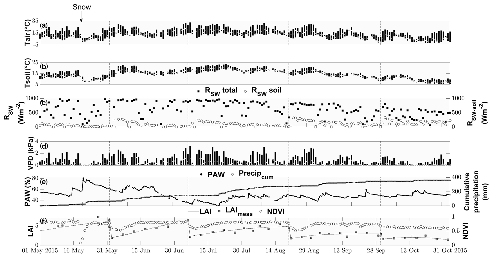
Figure 1Seasonal cycle of ancillary variables. Daily minimum, maximum and median (a) air and (b) soil temperatures (∘C) indicated by the lower and upper end of the bars and the white circle, respectively. (c) Daily maximum incident shortwave radiation (W m−2) reaching the top of the canopy (black squares) and reaching the soil surface (white circles). (d) Daily minimum, maximum and median vapor pressure deficit (kPA) indicated by the lower and upper end of the bars and the white circle, respectively. (e) Plant-available water (%) depicted by black squares and cumulative precipitation (mm) depicted by open circles. (f) Modeled leaf area index (black lines), measured LAI (gray squares) and normalized difference vegetation index (open circles).

Figure 2The response of the daily midday medians of NDVI (yellow circles), COS (green circles) and CO2 (orange circles) ecosystem fluxes around the four cutting events (a–d) of the grassland. The error bars depict the respective median absolute deviations. The cuts are marked by a dashed red line.
3.2 COS mole fractions above and within the canopy
While the canopy depleted the ambient χCOS during day as well as at night, we found that the χCOS reached values as low as 134 ppt (depletion of 102 ppt with respect to the mole fraction at canopy height) during nighttime (see Fig. 3) at the bottom of the canopy in contrast to the midday χCOS, which only went down to 389 ppt (depletion of 125 ppt with respect to the mole fraction at canopy height). We observed a decrease in (up to 26 ppm) within the uppermost layers of the canopy compared to at canopy height during daytime, while increased within the lowest layers compared to at the canopy height due to soil respiration. The above canopy χCOS increased considerably starting at the onset of the day and reached 587 ppt at 16:00 with a steep increase until 11:00 CET. Over the course of the season the midday ambient χCOS decreased from 500±28 ppt from mid-June to mid-July to 405±29 ppt in October, with the trend of increasing χCOS starting at the end of September (see Fig. S6).
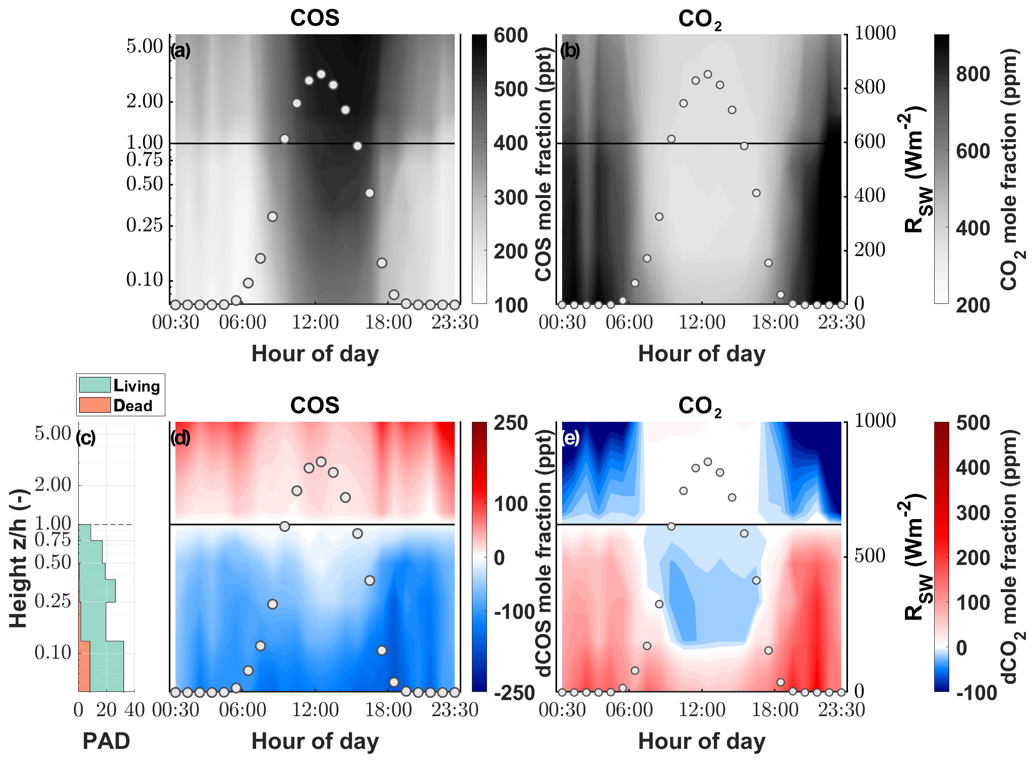
Figure 3Vertical gradient of the (a) COS and (b) CO2 mole fraction (parts per trillion and parts per million, respectively) depicted by the background color between the soil and the eddy covariance tower at 250 cm for 1 d. The left y axis shows the log of the measurement divided by the canopy height (z∕h). The white circles depict the incoming shortwave radiation (RSW; W m−2). Plant area density (PAD) split into living (green) and dead (orange) plant material (c). Vertical gradient of the difference between the mole fraction at canopy height and each measurement height for (d) COS and (e) CO2.
3.3 COS soil flux
The fluxes resulting from the soil chamber measurements ranged from −6.3 to 40.9 pmol m−2 s−1, with positive fluxes denoting emission (see Fig. 4d).
During nighttime (RSW = 0, n=43), 74.4 % of the COS fluxes were negative, implying that the soil of the grassland acted as a net sink for COS (range of −4.4 to 6.9 pmol m−2 s−1), whereas soils transitioned to a source in 88.5 % of all daytime measurements (RSW>0, n=200), reaching the highest fluxes of 40.9 pmol m−2 s−1 during midday (see Figs. 4a–c and S3). This diel pattern was maintained over the course of the season, however with decreasing maximum COS source strength of the soil towards the end of the season (Figs. 4a–c and S3). The random forest regression revealed that the most important variable for predicting the soil fluxes was the incident shortwave radiation reaching the soil surface (RSW−soil), accounting for more than 73.53 % of the total variance explained by the final model, while SWC and Tsoil only accounted for 17.84 % and 8.62 %, respectively. The fast response of the COS soil fluxes to changes in RSW can be seen in Fig. 4a, where we observed a decrease in RSW−soil as well as the COS soil flux during a cloudy period, even when the soil temperature still increased. Soil fluxes estimated with the random forest regression ranged from −1.3 to 5.0 pmol m−2 s−1, reflecting the fact that under real-world conditions very little solar radiation reaches the soil surface (Fig. 4e). The resulting emissions peaked during daytime shortly after the cuts, when a high proportion of incident radiation was reaching the soil surface, while simulated nighttime fluxes were dominated by uptake (in 93 % of all cases) for the whole season.
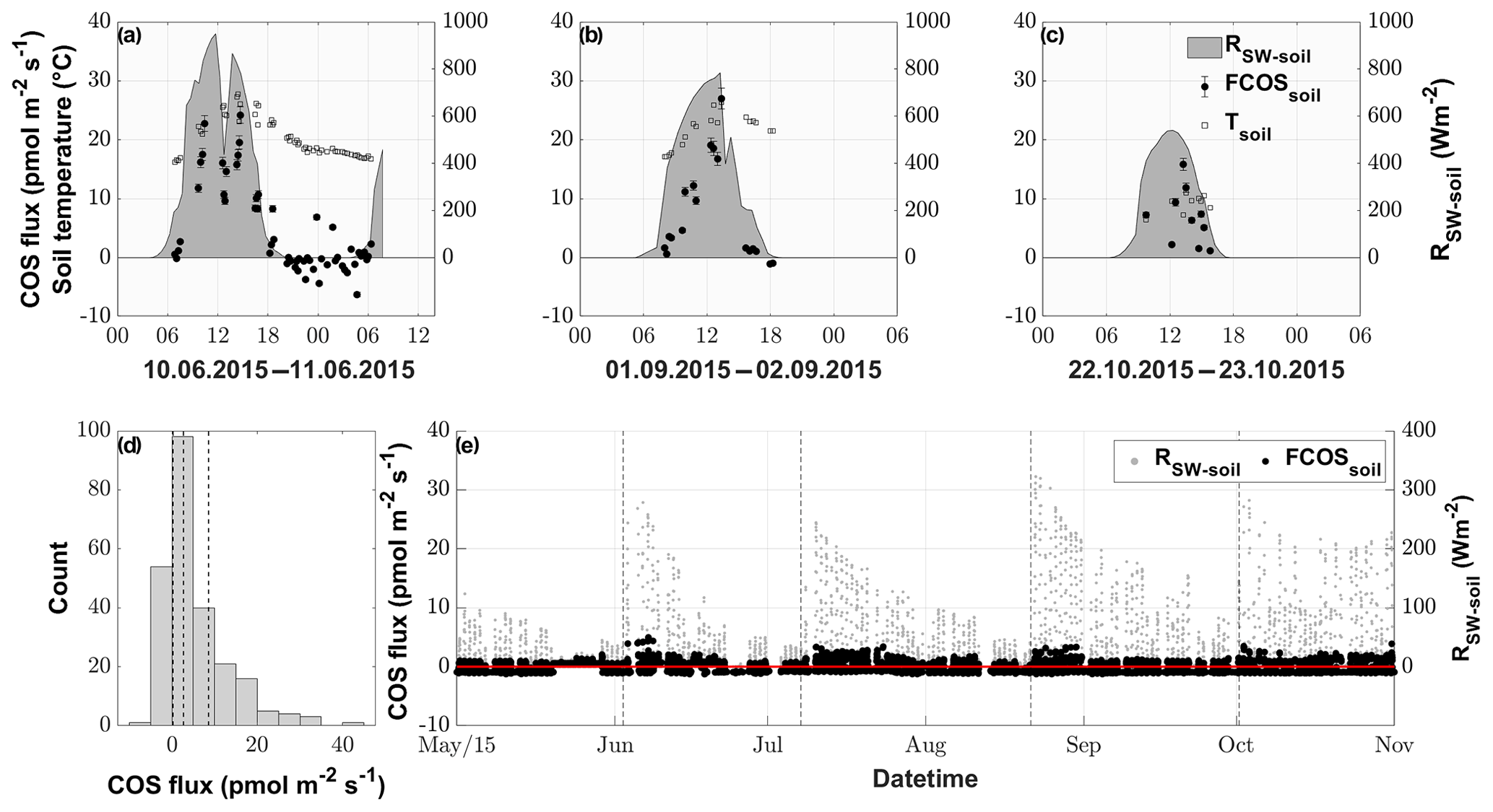
Figure 4COS soil fluxes (pmol m−2 s−1) originating from manual chamber measurements of 3 selected days, (a), (b) and (c), depicted by black circles; incident shortwave radiation reaching the soil (RSW−soil), depicted by the gray area; and soil temperature (Tsoil), depicted by empty black bordered squares. (d) Histogram of all conducted COS soil chamber observations, with the dashed vertical lines depicting the 25 %, 50 % and 75 % quantiles. (e) Season plot of the modeled COS soil fluxes (FCOSsoil), depicted by the black circles; incident shortwave radiation reaching the soil surface (RSW−soil), depicted by gray circles; and the black dashed lines depicting the cuttings of the grassland.
3.4 COS and CO2 ecosystem-scale fluxes
The grassland acted as a net sink for COS during the majority of our study period, with 80 % of the COS ecosystem fluxes between −56.0 and −4.5 pmol m−2 s−1 during daytime and −37.8 and 9.2 pmol m−2 s−1 during nighttime. We observed a net release of COS at the field site 11.2 % of the time. The net CO2 fluxes ranged from −20.4 to 4.8 µmol m−2 s−1 and −30.3 to 36.4 µmol m−2 s−1 for 80 % of all observations during daytime and nighttime, with daytime net emissions occurring after the cuttings of the grassland (Figs. 2a–c and 5a). While the COS nighttime fluxes remained unaffected by the cuts (Fig. 5c), the daytime fluxes showed a high variability (see Fig. 5b). Especially after the cuts, we observed a strong decline in COS uptake (Fig. 4b), and the grassland even turned into a net source for COS during middays (Fig. 2a–c), with a maximum emission flux of 26.8 pmol m−2 s−1 (midday median) in August after the cut. We observed COS emissions for up to 8 d after the cut, when the dried litter had already been removed (Fig. 2a–c). Compared to respiration processes outpacing GPP almost instantaneously after the cuts, the grassland reached its peak COS emission on the day of the cut only in July, whereas the peak was reached 5 d after the cut in June and August (Fig. 2a–c). The cut in October led to a reduction in COS uptake, which declined across several days and did not recover as the end of the season was reached (Figs. 2d and 5b). After the fertilization of the field in October, the grassland also turned into a source for COS during midday hours for 1 d (Fig. 5b). Our flux measurements also included a time when the grassland was covered with snow (on 20 May 2015), which reduced the COS (and CO2) fluxes to values close to zero. Over the course of the season, we observed a decline in the magnitude of the daytime COS uptake from pmol m−2 s−1 during midday in the first week of May down to pmol m−2 s−1 in the last week of October, which was also correlated with the decline in the CO2 sink strength from to µmol m−2 s−1 (Fig. 5a–b). We observed an increase in COS and CO2 fluxes within the growing phases after the cuts only up to an LAI of ∼4 (m2 m−2; Figs. S4–S5), which then leveled out for COS and declined for CO2 due to ecosystem-respiration-compensating GPP.
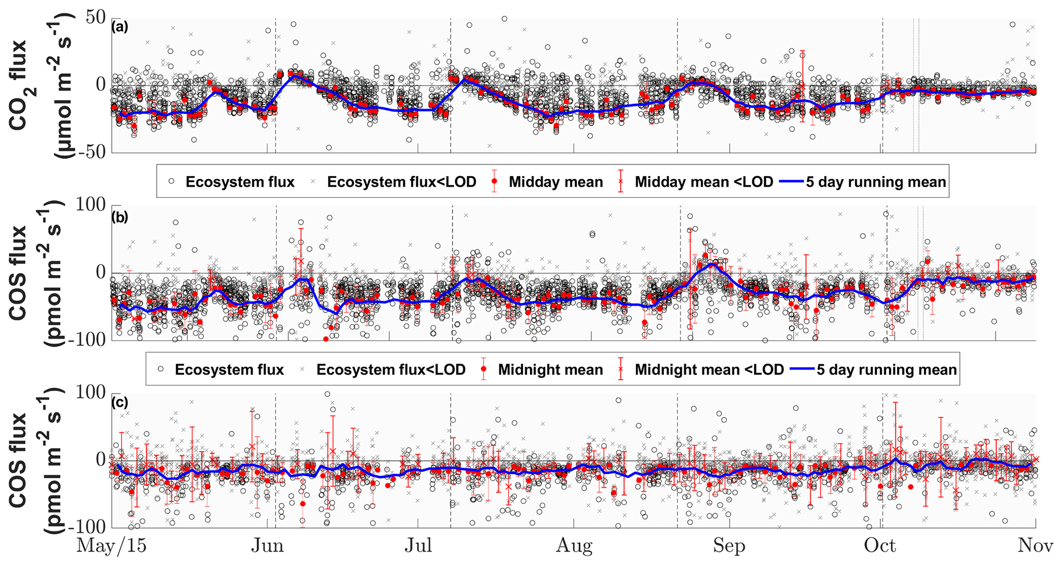
Figure 5Seasonal cycle of the half-hourly CO2 (a), COS daytime (b) and COS nighttime (c) ecosystem fluxes in micromoles per square meter per second and picomoles per square meter per second, depicted by black circles if they are above the limit of detection (LOD) and gray ×'s if they are below (Langford et al., 2015). The red circles depict the mean fluxes between 11:00 and 14:00 CET for (a) and (b) and between 23:00 and 02:00 for (c) that are above the LOD, while the red ×'s indicate means below the LOD. The red error bars depict the ±1 standard deviation of the mean. The blue lines depict the running mean (5 d) for the mean fluxes. The dashed black lines depict the cuttings of the grassland.
The seasonal pattern of a decrease in COS sink strength was similar for nighttime fluxes ( to pmol m−2 s−1; Fig. 5c). The mean nighttime respiration also decreased over the course of the season from 15.9±28.2 to 9.4±17.5 µmol m−2 s−1 between May and October (Fig. 5a).
Periods between May and August of low (after cuts) and high (before cuts) LAI were compared as diel courses (Fig. 5). Over the course of the day, both periods were characterized by a mean uptake of COS (Fig. 6c and d). Even though the uptake was similar during nighttime, the daytime pattern differed considerably. The modeled contribution of the soil to the ecosystem-scale COS flux under high LAI conditions (Fig. 6d) was minor, contributing 1.3 %, 5.5 % and 5.7 % of the ecosystem flux during midday, morning and evening, respectively. In contrast, during low LAI conditions the soil contribution to the ecosystem fluxes increased during daytime and contributed up to 82.4 % of the mean hourly COS ecosystem flux (Fig. 6c). While the grassland acted as a stronger sink for COS during daytime at a high LAI, reaching peak mean uptake values of up to pmol m−2 s−1 during midday, the mean daytime sink strength weakened, and we observed close to zero fluxes during midday in periods of low LAI. The magnitude of the soil flux (2±1 pmol m−2 s−1) was not high enough to explain the difference of up to 26.0 pmol m−2 s−1 between the measured COS ecosystem flux and COS flux resulting from the FP+ model (Fig. 6c), suggesting a missing COS source. For phases of high LAI, we saw a good agreement between hourly averaged modeled and measured COS ecosystem fluxes (Fig. 6d). While the grassland acted as a net sink for CO2 during periods of high LAI (Fig. 6b), a combination of a decline in GPP and an increase in daytime RECO turned it into a net source during midday in periods of low LAI as more incoming radiation was heating the soil surface (Fig. 6a).
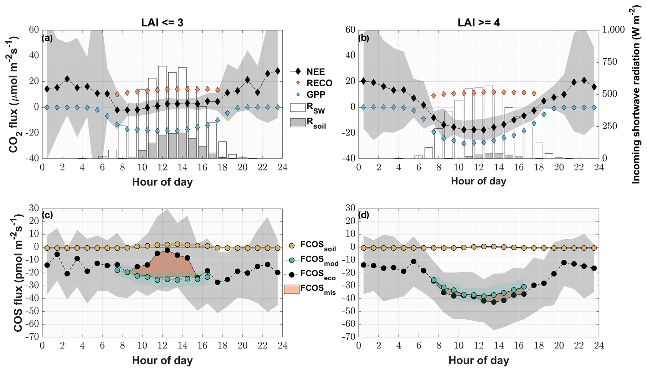
Figure 6Mean diel variation in the measured and modeled CO2 (a, b) and COS (c, d) fluxes for phases of low (LAI < = 3) (a, c) and high (LAI > = 4) LAI (b, d) from May to August. The diamonds depict the modeled gross primary productivity (blue), the modeled ecosystem respiration (orange) and the measured CO2 ecosystem fluxes (black) in micromoles per square meter per second. The circles depict the modeled COS soil flux (yellow), the modeled COS ecosystem flux (turquoise) and the measured COS ecosystem fluxes (black) in picomoles per square meter per second. The red area depicts the difference between the measured ecosystem flux and the sum of the modeled fluxes. The gray areas depict the ±1 standard deviation of the mean for all the measured fluxes. The white bars depict the diel mean total incoming shortwave radiation (W m−2), while the gray bars indicate the diel mean shortwave radiation reaching the soil surface.
3.5 Leaf and ecosystem relative uptake
The LRU at high-light conditions, ι, which we calculated using the FP+ algorithm, increased from relatively stable precut levels of 0.9–1.0 (–) before the second and the first cut to up to 1.6 (–) after the fourth cut (Fig. 7a). After the decrease in ι between the second and the third cut, ι increased steadily until the fourth cut, with the third cut seemingly not having an effect. The reason for the increase in ι after the second and fourth cut was a stronger decrease in GPP than the COS uptake, while both decreased more evenly after the third cut (Fig. 7b). We observed ι in the period before the fourth cut to be influenced not only by a decrease in COS uptake but also by a decrease in COS mole fraction (Fig. 7b). The mean midday ERUs varied between 2.0±0.1 (–) before and 4.5±0.4 (–) after the cuts. The larger difference between the ERU and ι after the cuts reflects that we observed similar respiration rates at low and high LAI (Fig. 6a–b).
Under low-light conditions, the LRU increased during pre- and postcut phases in a similar manner, with the last 15 d period in October showing an earlier increase in the morning and evening (see Fig. S7).

Figure 7(a) The seasonal cycle of ι (black line) with the 95 % confidence interval (gray area) resulting from the FP+ model and the midday mean (11:00–14:00 at PAR > 800 µmol m−2 s−1) ecosystem relative uptake (ERU; blue line) using the CO2 ecosystem flux for the calculation windows (∼15 d adjusted to cuts). The dashed black line depicts the progression of the leaf area index (LAI) of the grassland. (b) The contribution of the drivers (FCOS, χCOS, GPP and ) to the changes in ι between all calculation windows and the reference period (DOY 169–188) resulting from the linear perturbation analysis compared to the observed change in ι (δι).
4.1 COS mole fractions
The continuous seasonal decrease in above-canopy χCOS was within the range of published records observing mole fractions to decrease from 465 (in summer) to 375 ppt (in winter; Kuhn et al., 1999). This pattern is typical for the Northern Hemisphere and the COS drawdown by terrestrial ecosystems (Montzka et al., 2007). We found the lowest χCOS at the end of September, which coincides with the lowest ambient mole fractions of COS, measured in Ireland at the closest COS observation site, Mace Head (MHD), of the NOAA on 6 October (Fig. S6).
The extremely low COS canopy mole fractions we observed within the canopy have also been reported by Rastogi et al. (2018), who measured a mean χCOS minimum of 152 ppt at 1 m above the soil within an old-growth forest. Compared to the consistent decrease in COS below the canopy level during daytime and nighttime, the gradient for CO2 reverses during nighttime due to ongoing respiration processes while plants are not photosynthetically active. Even though the COS mole fraction at the layer closest to the soil was higher during the day than during nighttime, the absolute decrease in COS was lower during nighttime due to partial stomatal closure (Kooijmans et al., 2017; Campbell et al., 2017). The absolute difference in concentrations during daytime and nighttime originate from changes in the height of the planetary boundary layer (PBL). While the PBL is shallow during nighttime, and the COS mole fraction decreases due to sink strength of the grassland, at the onset of the day the PBL layer height increases fast, and COS-rich air is transported down to the ecosystem (Fig. S12; Campbell et al., 2017). A similarly steep increase until midday has also been observed by Rastogi et al. (2018). Even though CO2 and COS share a similar pathway into plants, reflected by their respective decrease in the mole fractions within the canopy, we saw a difference at the lower levels of our gradient analysis during daytime. We only observed an increase in CO2 mole fractions, caused by the release of CO2 through respiration processes in the soil, whereas COS mole fractions further declined down to the soil surface. This supports our soil model, which predicted only minor COS fluxes under conditions of high LAI, when only a small portion of incident radiation reaches the soil surface.
4.2 Soil fluxes
The nighttime soil chamber measurements compare well in terms of magnitude with the COS fluxes resulting from studies using dark chambers at agricultural and grassland sites (Whelan et al., 2018; Maseyk et al., 2014; Whelan and Rhew, 2016; Liu et al., 2010) and indicate the soil to be a small sink for COS. The current understanding of COS soil exchange links the COS consumption to soil biota, e.g., bacteria and fungi, possessing the ubiquitous enzyme CA (Kesselmeier et al., 1999; Meredith et al., 2019). The origin of COS in soils on the other hand is still highly debated, but comparisons of untreated and sterilized soils suggest yet unknown abiotic processes (Meredith et al., 2019; Kitz et al., 2019).
The high COS emissions resulting from the soil chambers during daytime lie at the upper end of the recently stated values of agricultural and grassland sites (Whelan et al., 2018; Kitz et al., 2017; Maseyk et al., 2014; Liu et al., 2010). This can partly be attributed to the type of chambers we used and their deployment. We allowed the full spectrum of incoming radiation to reach the soil surface, whereas most other studies used dark chambers. Therefore we were able to capture the influence of COS emission processes coupled to thermo- and photoproduction on our COS soil fluxes (Whelan and Rhew, 2015; Kitz et al., 2019; Meredith et al., 2018). This also led to lower peak soil emissions of COS at the end of the season, when the incoming radiation declined.
The low COS mole fractions observed in the lowermost canopy layers just above the soil surface emphasize the importance of using air from within the canopy for soil chamber measurements and not COS-richer air from above the canopy, which would increase the COS gradient and thus increase the uptake and decrease emission of COS to and from the soil.
Our modeled COS soil fluxes peak at about 12 % of the maximum emissions retrieved from the soil chambers. This is due to the difference in incident radiation reaching the soil surface between the fluxes resulting from chamber measurements and our model. For the chambers, the aboveground biomass was removed, whereas our modeled fluxes were adjusted for undisturbed canopy conditions.
Another factor contributing to the high-COS soil emissions might be the yearly fertilization using slurry as high-nitrogen content in soils has been linked to a higher source strength of COS (Kaisermann et al., 2018). This agrees well with the study of Kitz et al. (2019), who found a correlation between increased soil nitrogen content and soil COS emission in a laboratory experiment, with samples taken from the grassland on two different dates (i.e., June and September).
4.3 Ecosystem fluxes
Our observations show that the agriculturally used grassland acted as a major sink for COS during the growing season. The fluxes fit well within or even exceeded the COS uptake rates of published grassland and agricultural sites during their growing phases (Billesbach et al., 2014; Whelan and Rhew, 2016; Geng and Mu, 2004). The late snow event that occurred in the peak growing season almost completely inhibited the exchange of CO2 and COS as the snow acted as a diffusion barrier for these compounds (Björkman et al., 2010).
The cuttings and the consecutive drying of the above ground plant material at the site had a major influence on the COS exchange. COS emissions of a similar magnitude have also been reported at agricultural fields in phases of senescence (Maseyk et al., 2014; Billesbach et al., 2014). Although the soil was a strong source for COS, caused by the high Rsoil and Tsoil (Whelan and Rhew, 2015; Kitz et al., 2019; Meredith et al., 2018), and the sink strength of the grassland was low due to the reduced aboveground biomass, soil fluxes did not explain the emission on an ecosystem level (see Fig. 6a). As plants contain precursors involved in COS emission processes, e.g., methionine and cysteine (Meredith et al., 2018), the plant litter and dying plant parts remaining at the site after the cuts might be the missing source of COS. Laboratory tests of the soil of the grassland have shown that a mixing of dried litter and soil lead to a strong but short-lived emission peak of COS (Kitz et al., 2019). We did not observe strong COS emissions after the last cut as the incoming solar radiation, which we hypothesize to amplify the degradation of sulfur-containing compounds of plants, was reduced at the end of the season. Alternatively, the cutting of the grassland might induce stress-mediated COS production in the remaining living plant parts (Bloem et al., 2012; Gimeno et al., 2017). The delay in the peak COS emissions on the ecosystem scale after the cuts could indicate that some yet unknown biotic or abiotic processes take several days to release COS.
The short-lived COS emission by yet unknown biotic or abiotic processes after the fertilization of the grassland towards the end of the growing season was likely triggered by the increase in available nitrogen (Kaisermann et al., 2018) and COS precursors introduced to the soil in the form of cattle slurry (Hörtnagl et al., 2018).
Due to the independence of CA to catalyze COS without RPAR (Stimler et al., 2011), the grassland remained a sink for COS during nighttime. Again, the soil sink was too small to explain the total COS exchange (Fig. 6), which indicates that the plant stomata were not fully closed (Kooijmans et al., 2017) and were responsible for the majority of the COS uptake. The minimum or residual stomatal conductances at the field site in Neustift have been reported to be between 10 and 65 mmol m−2 s−1, depending on the species (Wohlfahrt, 2004).
The large variability in COS nighttime fluxes (Fig. 5c) is due to the combination of low wind speeds and stable stratification, which results in highly intermittent CO2 (Wohlfahrt et al., 2005) and COS fluxes compared to daytime. On a half-hourly basis, even a nighttime net uptake of CO2 has been reported at the field site, which is typically compensated for by large CO2 emissions in a subsequent averaging period (Wohlfahrt et al., 2005). We also observed this pattern for COS.
Although we observed phases of high VPD and low SWC (Fig. 1), they did not lead to a decrease in CO2 and COS ecosystem fluxes (Figs. S1–S2 in the Supplement), which has already been observed for the grassland CO2 and H2O fluxes between 2001 and 2009. The species located at the site were insensitive to progressive drought conditions (Brilli et al., 2011).
4.4 LRU
The parameter ι of this study is placed at the lower end of a recent compilation of published leaf-level LRUs that put 95 % of all data between 0.7 (–) and 6.2 (–), with a median of 1.7 (–; Whelan et al., 2018), which is lower than the LRU of 2.53 (–) estimated for grasslands by Seibt et al. (2010). Even the higher ι after the cuts was low compared to these studies. The seasonal trend of ι was strongly influenced by the cutting of the grass and can be attributed mainly to changes in the ratio of COS uptake to GPP. However, we also observed a strong decline in the ambient mole fraction of COS, which also had an equally strong influence on the change in ι as the COS flux for the 15 d window before the last cut (Fig. 7b).
Even though the changes in ι can be explained, it is important to keep in mind that the grassland was a source for COS on an ecosystem level after the cuts. For the calculation of LRUs we had to remove the canopy flux data containing COS and/or CO2 emissions since they would yield negative values for ERU and LRU (see Eq. 8). This indicates that the unknown source strength after cuts likely decreases the postcut ι's.
Due to the management interventions at the grassland site, the leaf area development was decoupled from seasonal changes in environmental forcing. This allowed us to measure concurrent CO2 and COS fluxes at the soil and ecosystem level for multiple growing periods within one season. The LAI on a seasonal scale as well as incoming solar radiation on hourly to seasonal scales determined whether soils were a source or a sink for COS. The incoming shortwave radiation reaching the soil surface had a decisive influence on the COS soil surface flux and thus supports our hypothesis H4. The covariance between the daytime CO2 and COS fluxes on a daily to seasonal level was high, and the fluxes only diverged after the cuts, leading to higher LRUs. Beside the perturbations of the ecosystem, the sink strength of the grassland was high for COS and declined over the course of the season (H1). The COS emissions on the ecosystem scale shortly after the cuts, which could not be explained by the soil source, raise questions about other unknown mechanisms of COS production within ecosystems (H2). With the exception of short periods after the cuts, the LRUs under high-light conditions were relatively constant during the season, indicating a good correlation between the COS flux and GPP under stable conditions (H3).
Data and materials are available at https://doi.org/10.5281/zenodo.3675078 (Spielmann et al., 2020).
The supplement related to this article is available online at: https://doi.org/10.5194/bg-17-4281-2020-supplement.
GW developed the concept of this study. GW acquired the funding for the project, leading to this publication. GW was responsible for the project administration. The planning and execution were supervised by GW. FMS, AH and FK were involved in the data curation. FMS, AH and FK conducted formal analyses. The investigation was done by FMS, AH, FK, KG and GW. The methodology was developed by GW, FMS and FK. The software was written by FMS, AH, FK, KG and GW. FMS visualized the data. All authors participated in writing and editing the paper.
The authors declare that they have no conflict of interest.
This study was financially supported by the Austrian National Science Fund (FWF; contracts P26931, P27176 and I03859), the Tyrolean Science Fund (contract UNI-0404/1801) and the University of Innsbruck (infrastructure funding by Research Area Alpine Space – Man and Environment to Georg Wohlfahrt). Financial support to Felix M. Spielmann was provided through a PhD scholarship by the University of Innsbruck. We thank Hofer family (Neustift, Austria) for kindly granting us access to the study site. COS flask data were provided by the Global Monitoring Division of the National Oceanic and Atmospheric Administration's Earth System Research Laboratory (NOAA ESRL/GMD).
This study was financially supported by the Austrian National Science Fund (FWF; contracts P26931, P27176 and I03859), the Tyrolean Science Fund (contract UNI-0404/1801) and the University of Innsbruck (infrastructure funding by Research Area Alpine Space Man and Environment to Georg Wohlfahrt). Financial support to Felix M. Spielmann was provided through a PhD scholarship by the University of Innsbruck.
This paper was edited by Martin De Kauwe and reviewed by Roisin Commane and two anonymous referees.
Asaf, D., Rotenberg, E., Tatarinov, F., Dicken, U., Montzka, S. A., and Yakir, D.: Ecosystem photosynthesis inferred from measurements of carbonyl sulphide flux, Nat. Geosci., 6, 186–190, https://doi.org/10.1038/ngeo1730, 2013.
Aubinet, M., Grelle, A., Ibrom, A., Rannik, U., Moncrieff, J., Foken, T., Kowalski, A. S., Martin, P. H., Berbigier, P., Bernhofer, C., Clement, R., Elbers, J., Granier, A., Grunwald, T., Morgenstern, K., Pilegaard, K., Rebmann, C., Snijders, W., Valentini, R., and Vesala, T.: Estimates of the annual net carbon and water exchange of forests: The EUROFLUX methodology, Adv. Ecol. Res., 30, 113–175, 2000.
Baldocchi, D.: Measuring fluxes of trace gases and energy between ecosystems and the atmosphere – the state and future of the eddy covariance method, Glob. Change Biol., 20, 3600–3609, https://doi.org/10.1111/gcb.12649, 2014.
Barr, A. G., Richardson, A. D., Hollinger, D. Y., Papale, D., Arain, M. A., Black, T. A., Bohrer, G., Dragoni, D., Fischer, M. L., Gu, L., Law, B. E., Margolis, H. A., McCaughey, J. H., Munger, J. W., Oechel, W., and Schaeffer, K.: Use of change-point detection for friction-velocity threshold evaluation in eddy-covariance studies, Agr. Forest Meteorol., 171, 31–45, https://doi.org/10.1016/j.agrformet.2012.11.023, 2013.
Billesbach, D. P., Berry, J. A., Seibt, U., Maseyk, K., Torn, M. S., Fischer, M. L., Abu-Naser, M., and Campbell, J. E.: Growing season eddy covariance measurements of carbonyl sulfide and CO2 fluxes: COS and CO2 relationships in Southern Great Plains winter wheat, Agr. Forest Meteorol., 184, 48–55, https://doi.org/10.1016/j.agrformet.2013.06.007, 2014.
Björkman, M. P., Morgner, E., Cooper, E. J., Elberling, B., Klemedtsson, L., and Björk, R. G.: Winter carbon dioxide effluxes from Arctic ecosystems: An overview and comparison of methodologies, Global Biogeochem. Cy., 24, GB3010, https://doi.org/10.1029/2009gb003667, 2010.
Bloem, E., Haneklaus, S., Kesselmeier, J., and Schnug, E.: Sulfur Fertilization and Fungal Infections Affect the Exchange of H2S and COS from Agricultural Crops, J. Agr. Food Chem., 60, 7588–7596, https://doi.org/10.1021/jf301912h, 2012.
Brilli, F., Hörtnagl, L., Hammerle, A., Haslwanter, A., Hansel, A., Loreto, F., and Wohlfahrt, G.: Leaf and ecosystem response to soil water availability in mountain grasslands, Agr. Forest Meteorol., 151, 1731–1740, https://doi.org/10.1016/j.agrformet.2011.07.007, 2011.
Brühl, C., Lelieveld, J., Crutzen, P. J., and Tost, H.: The role of carbonyl sulphide as a source of stratospheric sulphate aerosol and its impact on climate, Atmos. Chem. Phys., 12, 1239–1253, https://doi.org/10.5194/acp-12-1239-2012, 2012.
Campbell, J. E., Whelan, M. E., Berry, J. A., Hilton, T. W., Zumkehr, A., Stinecipher, J., Lu, Y., Kornfeld, A., Seibt, U., Dawson, T. E., Montzka, S. A., Baker, I. T., Kulkarni, S., Wang, Y., Herndon, S. C., Zahniser, M. S., Commane, R., and Loik, M. E.: Plant Uptake of Atmospheric Carbonyl Sulfide in Coast Redwood Forests, J. Geophys. Res.-Biogeo., 122, 3391–3404, https://doi.org/10.1002/2016jg003703, 2017.
Ensign, S. A.: Reactivity of Carbon Monoxide Dehydrogenase from Rhodospirillum rubrum with Carbon Dioxide, Carbonyl Sulfide, and Carbon Disulfide, Biochemistry, 34, 5372–5381, https://doi.org/10.1021/bi00016a008, 1995.
Geng, C. and Mu, Y.: Carbonyl sulfide and dimethyl sulfide exchange between lawn and the atmosphere, J. Geophys. Res.-Atmos., 109, D12302, https://doi.org/10.1029/2003jd004492, 2004.
Gerdel, K., Spielmann, F. M., Hammerle, A., and Wohlfahrt, G.: Eddy covariance carbonyl sulfide flux measurements with a quantum cascade laser absorption spectrometer, Atmos. Meas. Tech., 10, 3525–3537, https://doi.org/10.5194/amt-10-3525-2017, 2017.
Gimeno, T. E., Ogee, J., Royles, J., Gibon, Y., West, J. B., Burlett, R., Jones, S. P., Sauze, J., Wohl, S., Benard, C., Genty, B., and Wingate, L.: Bryophyte gas-exchange dynamics along varying hydration status reveal a significant carbonyl sulphide (COS) sink in the dark and COS source in the light, New Phytol., 215, 965–976, https://doi.org/10.1111/nph.14584, 2017.
Hörtnagl, L., Clement, R., Graus, M., Hammerle, A., Hansel, A., and Wohlfahrt, G.: Dealing with disjunct concentration measurements in eddy covariance applications: A comparison of available approaches, Atmos. Environ., 44, 2024–2032, https://doi.org/10.1016/j.atmosenv.2010.02.042, 2010.
Hörtnagl, L., Barthel, M., Buchmann, N., Eugster, W., Butterbach-Bahl, K., Díaz-Pinés, E., Zeeman, M., Klumpp, K., Kiese, R., Bahn, M., Hammerle, A., Lu, H., Ladreiter-Knauss, T., Burri, S., and Merbold, L.: Greenhouse gas fluxes over managed grasslands in Central Europe, Glob. Change Biol., 24, 1843–1872, https://doi.org/10.1111/gcb.14079, 2018.
Kaisermann, A., Jones, S., Wohl, S., Ogée, J., and Wingate, L.: Nitrogen Fertilization Reduces the Capacity of Soils to Take up Atmospheric Carbonyl Sulphide, Soil Syst., 2, 62, https://doi.org/10.3390/soilsystems2040062, 2018.
Kesselmeier, J., Teusch, N., and Kuhn, U.: Controlling variables for the uptake of atmospheric carbonyl sulfide by soil, J. Geophys. Res.-Atmos., 104, 11577–11584, https://doi.org/10.1029/1999jd900090, 1999.
Kitz, F., Gerdel, K., Hammerle, A., Laterza, T., Spielmann, F. M., and Wohlfahrt, G.: In situ soil COS exchange of a temperate mountain grassland under simulated drought, Oecologia, 183, 851–860, https://doi.org/10.1007/s00442-016-3805-0, 2017.
Kitz, F., Gómez-Brandón, M., Eder, B., Etemadi, M., Spielmann, F. M., Hammerle, A., Insam, H., and Wohlfahrt, G.: Soil carbonyl sulfide exchange in relation to microbial community composition: Insights from a managed grassland soil amendment experiment, Soil Biol. Biochem., 135, 28–37, https://doi.org/10.1016/j.soilbio.2019.04.005, 2019.
Kooijmans, L. M. J., Uitslag, N. A. M., Zahniser, M. S., Nelson, D. D., Montzka, S. A., and Chen, H.: Continuous and high-precision atmospheric concentration measurements of COS, CO2, CO and H2O using a quantum cascade laser spectrometer (QCLS), Atmos. Meas. Tech., 9, 5293–5314, https://doi.org/10.5194/amt-9-5293-2016, 2016.
Kooijmans, L. M. J., Maseyk, K., Seibt, U., Sun, W., Vesala, T., Mammarella, I., Kolari, P., Aalto, J., Franchin, A., Vecchi, R., Valli, G., and Chen, H.: Canopy uptake dominates nighttime carbonyl sulfide fluxes in a boreal forest, Atmos. Chem. Phys., 17, 11453–11465, https://doi.org/10.5194/acp-17-11453-2017, 2017.
Kooijmans, L. M. J., Sun, W., Aalto, J., Erkkilä, K. M., Maseyk, K., Seibt, U., Vesala, T., Mammarella, I., and Chen, H.: Influences of light and humidity on carbonyl sulfide-based estimates of photosynthesis, P. Natl. Acad. Sci. USA, 116, 2470–2475, https://doi.org/10.1073/pnas.1807600116, 2019.
Krysztofiak, G., Té, Y. V., Catoire, V., Berthet, G., Toon, G. C., Jégou, F., Jeseck, P., and Robert, C.: Carbonyl Sulphide (OCS) Variability with Latitude in the Atmosphere, Atmos. Ocean, 53, 89–101, https://doi.org/10.1080/07055900.2013.876609, 2015.
Kuhn, U., Ammann, C., Wolf, A., Meixner, F. X., Andreae, M. O., and Kesselmeier, J.: Carbonyl sulfide exchange on an ecosystem scale: soil represents a dominant sink for atmospheric COS, Atmos. Environ., 33, 995–1008, https://doi.org/10.1016/S1352-2310(98)00211-8, 1999.
Langford, B., Acton, W., Ammann, C., Valach, A., and Nemitz, E.: Eddy-covariance data with low signal-to-noise ratio: time-lag determination, uncertainties and limit of detection, Atmos. Meas. Tech., 8, 4197–4213, https://doi.org/10.5194/amt-8-4197-2015, 2015.
Lasslop, G., Reichstein, M., Papale, D., Richardson, A. D., Arneth, A., Barr, A., Stoy, P., and Wohlfahrt, G.: Separation of net ecosystem exchange into assimilation and respiration using a light response curve approach: critical issues and global evaluation, Glob. Change Biol., 16, 187–208, https://doi.org/10.1111/j.1365-2486.2009.02041.x, 2010.
Le Quéré, C., Andrew, R. M., Friedlingstein, P., Sitch, S., Pongratz, J., Manning, A. C., Korsbakken, J. I., Peters, G. P., Canadell, J. G., Jackson, R. B., Boden, T. A., Tans, P. P., Andrews, O. D., Arora, V. K., Bakker, D. C. E., Barbero, L., Becker, M., Betts, R. A., Bopp, L., Chevallier, F., Chini, L. P., Ciais, P., Cosca, C. E., Cross, J., Currie, K., Gasser, T., Harris, I., Hauck, J., Haverd, V., Houghton, R. A., Hunt, C. W., Hurtt, G., Ilyina, T., Jain, A. K., Kato, E., Kautz, M., Keeling, R. F., Klein Goldewijk, K., Körtzinger, A., Landschützer, P., Lefèvre, N., Lenton, A., Lienert, S., Lima, I., Lombardozzi, D., Metzl, N., Millero, F., Monteiro, P. M. S., Munro, D. R., Nabel, J. E. M. S., Nakaoka, S., Nojiri, Y., Padin, X. A., Peregon, A., Pfeil, B., Pierrot, D., Poulter, B., Rehder, G., Reimer, J., Rödenbeck, C., Schwinger, J., Séférian, R., Skjelvan, I., Stocker, B. D., Tian, H., Tilbrook, B., Tubiello, F. N., van der Laan-Luijkx, I. T., van der Werf, G. R., van Heuven, S., Viovy, N., Vuichard, N., Walker, A. P., Watson, A. J., Wiltshire, A. J., Zaehle, S., and Zhu, D.: Global Carbon Budget 2017, Earth Syst. Sci. Data, 10, 405–448, https://doi.org/10.5194/essd-10-405-2018, 2018.
Liaw, A. and Wiener, M.: Classification and Regression by RandomForest, R News, 2/3, 18–22, 2002.
Liu, J., Geng, C., Mu, Y., Zhang, Y., Xu, Z., and Wu, H.: Exchange of carbonyl sulfide (COS) between the atmosphere and various soils in China, Biogeosciences, 7, 753–762, https://doi.org/10.5194/bg-7-753-2010, 2010.
Lorimer, G. H. and Pierce, J.: Carbonyl sulfide: an alternate substrate for but not an activator of ribulose-1,5-bisphosphate carboxylase, J. Biol. Chem., 264, 2764–2772, 1989.
Maseyk, K., Berry, J. A., Billesbach, D., Campbell, J. E., Torn, M. S., Zahniser, M., and Seibt, U.: Sources and sinks of carbonyl sulfide in an agricultural field in the Southern Great Plains, P. Natl. Acad. Sci. USA, 111, 9064–9069, https://doi.org/10.1073/pnas.1319132111, 2014.
Meredith, L. K., Boye, K., Youngerman, C., Whelan, M., Ogee, J., Sauze, J., and Wingate, L.: Coupled Biological and Abiotic Mechanisms Driving Carbonyl Sulfide Production in Soils, Soil Syst., 2, 27, https://doi.org/10.3390/soilsystems2030037, 2018.
Meredith, L. K., Ogée, J., Boye, K., Singer, E., Wingate, L., von Sperber, C., Sengupta, A., Whelan, M., Pang, E., Keiluweit, M., Brüggemann, N., Berry, J. A., and Welander, P. V.: Soil exchange rates of COS and CO18O differ with the diversity of microbial communities and their carbonic anhydrase enzymes, ISME J., 13, 290–300, https://doi.org/10.1038/s41396-018-0270-2, 2019.
Montzka, S. A., Calvert, P., Hall, B. D., Elkins, J. W., Conway, T. J., Tans, P. P., and Sweeney, C.: On the global distribution, seasonality, and budget of atmospheric carbonyl sulfide (COS) and some similarities to CO2, J. Geophys. Res.-Atmos., 112, D09302, https://doi.org/10.1029/2006jd007665, 2007.
Notni, J., Schenk, S., Protoschill-Krebs, G., Kesselmeier, J., and Anders, E.: The missing link in COS metabolism: a model study on the reactivation of carbonic anhydrase from its hydrosulfide analogue, Chembiochem, 8, 530–536, https://doi.org/10.1002/cbic.200600436, 2007.
Ogawa, T., Noguchi, K., Saito, M., Nagahata, Y., Kato, H., Ohtaki, A., Nakayama, H., Dohmae, N., Matsushita, Y., Odaka, M., Yohda, M., Nyunoya, H., and Katayama, Y.: Carbonyl Sulfide Hydrolase from Thiobacillus thioparus Strain THI115 Is One of the β-Carbonic Anhydrase Family Enzymes, J. Am. Chem. Soc., 135, 3818–3825, https://doi.org/10.1021/ja307735e, 2013.
Protoschill-Krebs, G. and Kesselmeier, J.: ENZYMATIC PATHWAYS FOR THE CONSUMPTION OF CARBONYL SULFIDE (COS) BY HIGHER-PLANTS, Bot. Acta, 105, 206–212, 1992.
Rastogi, B., Berkelhammer, M., Wharton, S., Whelan, M. E., Itter, M. S., Leen, J. B., Gupta, M. X., Noone, D., and Still, C. J.: Large Uptake of Atmospheric OCS Observed at a Moist Old Growth Forest: Controls and Implications for Carbon Cycle Applications, J. Geophys. Res.-Biogeo., 123, 3424–3438, https://doi.org/10.1029/2018jg004430, 2018.
Sandoval-Soto, L., Stanimirov, M., von Hobe, M., Schmitt, V., Valdes, J., Wild, A., and Kesselmeier, J.: Global uptake of carbonyl sulfide (COS) by terrestrial vegetation: Estimates corrected by deposition velocities normalized to the uptake of carbon dioxide (CO2), Biogeosciences, 2, 125–132, https://doi.org/10.5194/bg-2-125-2005, 2005.
Seefeldt, L. C., Rasche, M. E., and Ensign, S. A.: Carbonyl sulfide and carbon dioxide as new substrates, and carbon disulfide as a new inhibitor, of nitrogenase, Biochemistry, 34, 5382–5389, https://doi.org/10.1021/bi00016a009, 1995.
Seibt, U., Kesselmeier, J., Sandoval-Soto, L., Kuhn, U., and Berry, J. A.: A kinetic analysis of leaf uptake of COS and its relation to transpiration, photosynthesis and carbon isotope fractionation, Biogeosciences, 7, 333–341, https://doi.org/10.5194/bg-7-333-2010, 2010.
Smeulders, M. J., Pol, A., Venselaar, H., Barends, T. R. M., Hermans, J., Jetten, M. S. M., and Op den Camp, H. J. M.: Bacterial CS2 Hydrolases from Acidithiobacillus thiooxidans Strains Are Homologous to the Archaeal Catenane CS2 Hydrolase, J. Bacteriol., 195, 4046, https://doi.org/10.1128/JB.00627-13, 2013.
Spielmann, F. M., Wohlfahrt, G., Hammerle, A., Kitz, F., Migliavacca, M., Alberti, G., Ibrom, A., El-Madany, T. S., Gerdel, K., Moreno, G., Kolle, O., Karl, T., Peressotti, A., and Delle Vedove, G.: Gross Primary Productivity of Four European Ecosystems Constrained by Joint CO2 and COS Flux Measurements, Geophys. Res. Lett., 46, 5284–5293, https://doi.org/10.1029/2019gl082006, 2019.
Spielmann, F. M., Hammerle, A., Kitz, F., Gerdel, K., and Wohlfahrt, G.: Dataset for “Seasonal dynamics of the COS and CO2 exchange of a managed temperate grassland”, Zenodo, https://doi.org/10.5281/zenodo.3675078, 2020.
Stimler, K., Berry, J. A., Montzka, S. A., and Yakir, D.: Association between Carbonyl Sulfide Uptake and (18)Delta during Gas Exchange in C-3 and C-4 Leaves, Plant Physiol., 157, 509–517, https://doi.org/10.1104/pp.111.176578, 2011.
Stoy, P. C., Katul, G. G., Siqueira, M. B. S., Juang, J. Y., Novick, K. A., McCarthy, H. R., Oishi, A. C., Uebelherr, J. M., Kim, H. S., and Oren, R.: Separating the effects of climate and vegetation on evapotranspiration along a successional chronosequence in the southeastern US, Glob. Change Biol., 12, 2115–2135, https://doi.org/10.1111/j.1365-2486.2006.01244.x, 2006.
Tucker, C. J.: Red and photographic infrared linear combinations for monitoring vegetation, Remote Sens. Environ., 8, 127–150, https://doi.org/10.1016/0034-4257(79)90013-0, 1979.
Whelan, M. E. and Rhew, R. C.: Carbonyl sulfide produced by abiotic thermal and photodegradation of soil organic matter from wheat field substrate, J. Geophys. Res.-Biogeo., 120, 54–62, https://doi.org/10.1002/2014jg002661, 2015.
Whelan, M. E. and Rhew, R. C.: Reduced sulfur trace gas exchange between a seasonally dry grassland and the atmosphere, Biogeochemistry, 128, 267–280, https://doi.org/10.1007/s10533-016-0207-7, 2016.
Whelan, M. E., Lennartz, S. T., Gimeno, T. E., Wehr, R., Wohlfahrt, G., Wang, Y., Kooijmans, L. M. J., Hilton, T. W., Belviso, S., Peylin, P., Commane, R., Sun, W., Chen, H., Kuai, L., Mammarella, I., Maseyk, K., Berkelhammer, M., Li, K.-F., Yakir, D., Zumkehr, A., Katayama, Y., Ogée, J., Spielmann, F. M., Kitz, F., Rastogi, B., Kesselmeier, J., Marshall, J., Erkkilä, K.-M., Wingate, L., Meredith, L. K., He, W., Bunk, R., Launois, T., Vesala, T., Schmidt, J. A., Fichot, C. G., Seibt, U., Saleska, S., Saltzman, E. S., Montzka, S. A., Berry, J. A., and Campbell, J. E.: Reviews and syntheses: Carbonyl sulfide as a multi-scale tracer for carbon and water cycles, Biogeosciences, 15, 3625–3657, https://doi.org/10.5194/bg-15-3625-2018, 2018.
Wohlfahrt, G.: Modelling fluxes and concentrations of CO2, H2O and sensible heat within and above a mountain meadow canopy: A comparison of three Lagrangian models and three parameterisation options for the Lagrangian time scale, Bound.-Lay. Meteorol., 113, 43–80, https://doi.org/10.1023/B:BOUN.0000037326.40490.1f, 2004.
Wohlfahrt, G., Bahn, M., Tappeiner, U., and Cernusca, A.: A multi-component, multi-species model of vegetation-atmosphere CO2 and energy exchange for mountain grasslands, Agr. Forest Meteorol., 106, 261–287, https://doi.org/10.1016/s0168-1923(00)00224-0, 2001.
Wohlfahrt, G., Anfang, C., Bahn, M., Haslwanter, A., Newesely, C., Schmitt, M., Drosler, M., Pfadenhauer, J., and Cernusca, A.: Quantifying nighttime ecosystem respiration of a meadow using eddy covariance, chambers and modelling, Agr. Forest Meteorol., 128, 141–162, https://doi.org/10.1016/j.agrformet.2004.11.003, 2005.
Wohlfahrt, G., Hammerle, A., Haslwanter, A., Bahn, M., Tappeiner, U., and Cernusca, A.: Seasonal and inter-annual variability of the net ecosystem CO2 exchange of a temperate mountain grassland: Effects of weather and management, J. Geophys. Res.-Atmos., 113, D08110, https://doi.org/10.1029/2007jd009286, 2008.
Wohlfahrt, G., Brilli, F., Hoertnagl, L., Xu, X., Bingemer, H., Hansel, A., and Loreto, F.: Carbonyl sulfide (COS) as a tracer for canopy photosynthesis, transpiration and stomatal conductance: potential and limitations, Plant Cell Environ., 35, 657–667, https://doi.org/10.1111/j.1365-3040.2011.02451.x, 2012.
Yang, F., Qubaja, R., Tatarinov, F., Rotenberg, E., and Yakir, D.: Assessing canopy performance using carbonyl sulfide measurements, Glob. Change Biol., 24, 3486–3498, https://doi.org/10.1111/gcb.14145, 2018.