Structure and function of epipelagic mesozooplankton and their response to dust deposition events during the spring PEACETIME cruise in the Mediterranean Sea

The PEACETIME cruise (May–June 2017) was a basin-scale survey covering the Provencal, Algerian, Tyrrhenian, and Ionian basins during the post-spring bloom period and was dedicated to tracking the impact of Saharan dust deposition events on the Mediterranean Sea pelagic ecosystem. Two such events occurred during this period, and the cruise strategy allowed for the study of the initial phase of the ecosystem response to one dust event in the Algerian Basin (during 5 d at the so-called “FAST long-duration station”) as well as the study of a latter response to another dust event in the Tyrrhenian Basin (by sampling from 5 to 12 d after the deposition). This paper documents the structural and functional patterns of the zooplankton component during this survey, including their responses to these two dust events. The mesozooplankton were sampled at 12 stations using nets with two different mesh sizes (100 and 200 µm) that were mounted on a Bongo frame for vertical hauls within the depth layer from 0 to 300 m.

The Algerian and Tyrrhenian basins were found to be quite similar in terms of hydrological and biological variables, which clearly differentiated them from the northern Provencal Basin and the eastern Ionian Basin. In general, total mesozooplankton showed reduced variations in abundance and biomass values over the whole area, with a noticeable contribution from the small size fraction (<500 µm) of up to 50 % with respect to abundance and 25 % with respect to biomass. This small size fraction makes a significant contribution (15 %–21 %) to the mesozooplankton fluxes (carbon demand, grazing pressure, respiration, and excretion), which is estimated using allometric relationships to the mesozooplankton size spectrum at all stations. The taxonomic structure was dominated by copepods, mainly cyclopoid and calanoid copepods, and was completed by appendicularians, ostracods, and chaetognaths. Zooplankton taxa assemblages, analyzed using multivariate analysis and rank frequency diagrams, slightly differed between basins, which is in agreement with recently proposed Mediterranean regional patterns.

However, the strongest changes in the zooplankton community were linked to the abovementioned dust deposition events. A synoptic analysis of the two dust events observed in the Tyrrhenian and Algerian basins, based on the rank frequency diagrams and a derived index proposed by Mouillot and Lepretre (2000), delivered a conceptual model of a virtual time series of the zooplankton community responses after a dust deposition event. The initial phase before the deposition event (state 0) was dominated by small-sized cells consumed by their typical zooplankton filter feeders (small copepods and appendicularians). The disturbed phase during the first 5 d following the deposition event (state 1) then induced a strong increase in filter feeders and grazers of larger cells as well as the progressive attraction of carnivorous species, leading to a sharp increase in the zooplankton distribution index. Afterward, this index progressively decreased from day 5 to day 12 following the event, highlighting a diversification of the community (state 2). A 3-week delay was estimated for the index to return to its initial value, potentially indicating the recovery time of a Mediterranean zooplankton community after a dust event.

To our knowledge, PEACETIME is the first in situ study that has allowed for the observation of mesozooplankton responses before and soon after natural Saharan dust depositions. The change in the rank frequency diagrams of the zooplankton taxonomic structure is an interesting tool to highlight short-term responses of zooplankton to episodic dust deposition events. Obviously dust-stimulated pelagic productivity impacts up to mesozooplankton in terms of strong but short changes in taxa assemblages and trophic structure, with potential implications for oligotrophic systems such as the Mediterranean Sea.

1 Introduction

The Mediterranean Sea is a semi-enclosed basin connected to the Atlantic Ocean and the Black Sea. It is composed of two major subbasins, the eastern and western Mediterranean, which are connected by the Sicilian Strait (Skliris, 2014). Due to its characteristics, such as its unique thermohaline circulation pattern and deep-water formation process, the Mediterranean Sea can be considered as a model of the world's oceans (Bethoux et al., 1999; Lejeusne et al., 2010). In addition, it is considered to be oligotrophic with an excess of carbon, a deficiency of phosphorus relative to nitrogen (Durrieu de Madron et al., 2011), and a decreasing west–east chlorophyll-a (Chl-a) gradient (i.e., Siokou-Frangou et al., 2010).

For the last 200 years, numerous investigations have documented the pelagic zooplankton community inhabiting the Mediterranean Sea (Saiz et al., 2014), including long-term time series (i.e., Fernández de Puelles et al., 2003; Mazzocchi et al., 2007; Molinero et al., 2008; García-Comas et al., 2011; Berline et al., 2012) and a succession of oceanographic surveys covering wide transects during different periods of the year (Kimor and Wood, 1975; Nowaczyk et al., 2011; Donoso et al., 2017; Siokou et al., 2019). The regular monitoring of the zooplankton community is essential when considering the high sensitivity of the Mediterranean Sea to anthropogenic and climate disturbance (Sazzini et al., 2014). Some of these disturbances may alter the structure and function of the pelagic ecosystem, and this is critical considering that marine ecosystems are being altered by anthropogenic climate change at an unprecedented rate (Chust et al., 2017).

Dust deposition is a major source of micro- and macro-nutrients (Wagener et al., 2010) that can stimulate primary production (Ridame et al., 2014), accelerate carbon sedimentation, and possibly accelerate the aggregation of marine particles (i.e., Neuer et al., 2004; Ternon et al., 2011; Bressac et al., 2014). Large amounts of Saharan dust can be transported in the atmosphere throughout the western and eastern Mediterranean Sea region and can then be deposited onto the sea surface by wet or dry deposition. The PEACETIME oceanographic cruise, carried out between 10 May and 11 June 2017, was designed to study the processes occurring in the Mediterranean Sea after atmospheric dust deposition in situ, including their impact on marine nutrient budget and fluxes and their affect on the biogeochemical function of the pelagic ecosystem. Thus, the survey strategy was designed to be flexible in order to be able to change the sampling area depending on atmospheric events (Guieu et al., 2020). Consequently, the survey sampling program realized consisted of 14 oceanographic stations in the central and western parts of the Mediterranean Sea.

The aims of the present contribution to the PEACETIME project are (1) to document the zooplankton abundance, biomass, and size distribution along the survey transect, paying special attention to small-sized zooplankton; (2) to analyze the relationship between zooplankton structure and environmental variability, including dust deposition; and (3) to estimate the bottom-up (nutrient regeneration) and the top-down (grazing) impact of zooplankton on phytoplankton stock and production by estimating its ingestion, respiration, and ammonium and phosphate excretions using allometric models.

These objectives will serve to test the following research questions:

1. Did the Saharan dust events impact the zooplankton community structure following deposition?

2. If the Saharan dust events did impact the zooplankton community structure, would the effect be immediately observable or would there be a lag time?

3. Would changes in zooplankton community structure driven by dust deposition exceed regional differences under oligotrophic conditions?

2 Material and methods

2.1 Study area and environmental variables

The PEACETIME cruise survey was conducted in May–June 2017 in the western Mediterranean Sea (Fig. 1) onboard the R/V POURQUOI PAS?. Among the 12 stations studied, 10 were sampled once for zooplankton (the short-duration stations ST1–ST9 and the long-duration station TYR), whereas two long-duration stations (ION and FAST, lasting 3 and 5 d, respectively) were sampled three times. The station positions along the transect were planned before the cruise in order to sample the principal ecoregions (see Fig. 4 in Guieu et al., 2020) with the exception of FAST, which was an opportunistic station to monitor a wet dust deposition event that occurred on 5 June – a few hours after the first sampling date (Table 1). A dust event occurred over a large area, including the southern Tyrrhenian Basin, starting on 10 May and could have impacted the samples at ST5, TYR, and ST6 which were sampled on 16, 19, and 22 May, respectively (Cécile Guieu, personal communication, 2020).

Table 1 Stations sampled during the PEACETIME survey: geographical information, date, and time of zooplankton net sampling. AB refers to the Algerian Basin, PB refers to the Provencal Basin, TB refers to the Tyrrhenian Basin, and IB refers to the Ionian Basin.

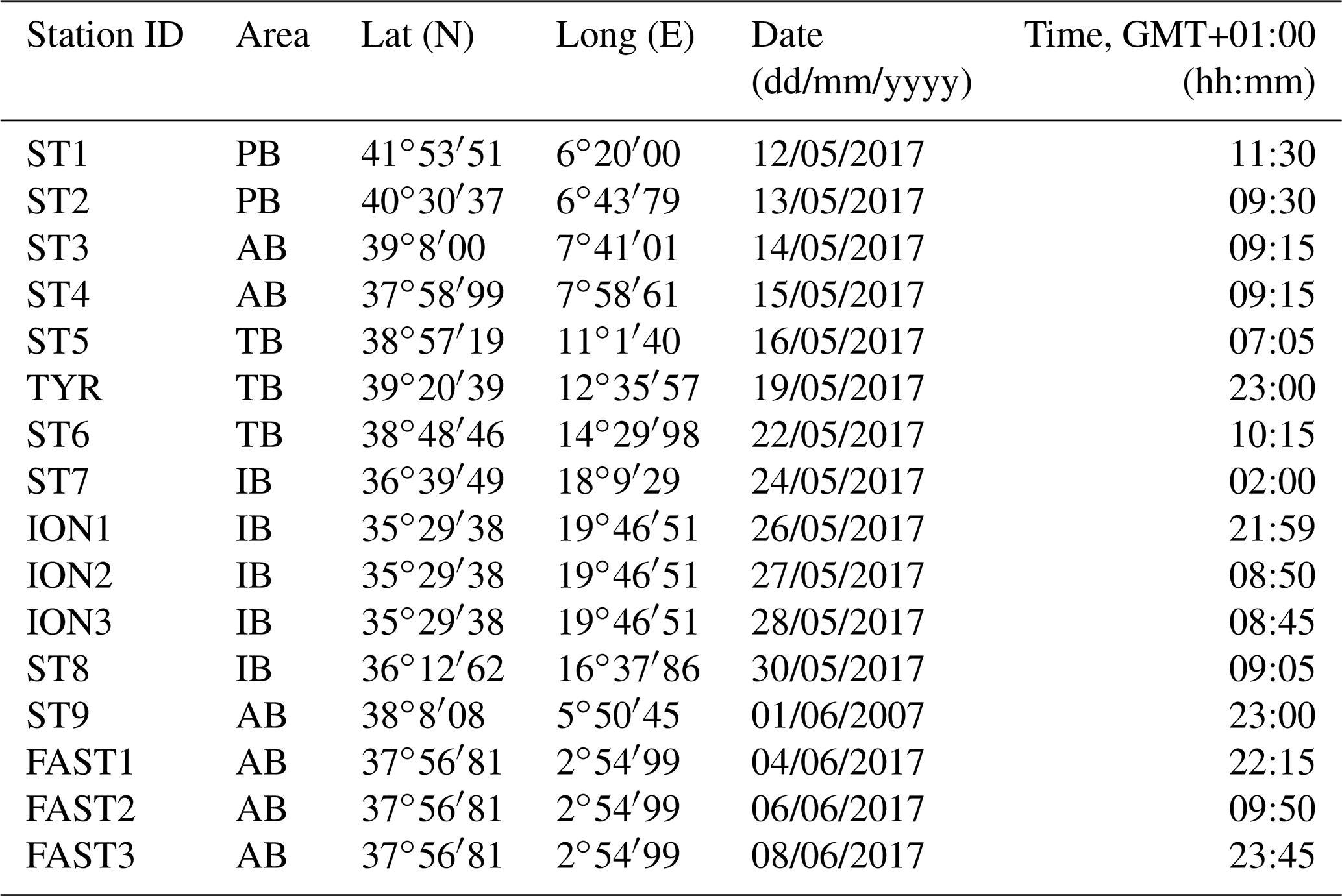
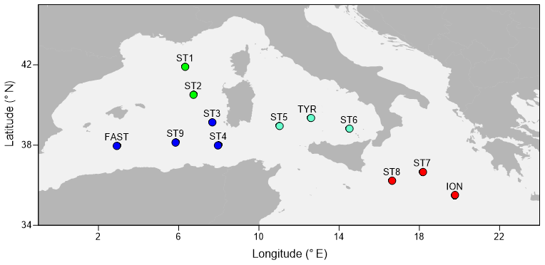
Figure 1 A map showing the sampling points during the PEACETIME cruise 2017. The colors of the points indicate the different areas considered over the course of the study: green dots denote the Provencal Basin (PB), dark blue dots denote the Algerian Basin (AB), light blue dots denote the Tyrrhenian Basin (TB), and red dots denote the Ionian Basin (IB).

Hydrological variables (temperature, density, and salinity) were measured on vertical profiles using a CTD (conductivity, temperature, and depth profiler). Dissolved oxygen was measured using a SBE43 sensor, and the Chl-a concentration was determined from Niskin bottle samples by high-performance liquid chromatography (HPLC), following the protocol of Ras et al. (2008), and with a fluorescence sensor coupled to the CTD. Primary production was measured using the ¹⁴C-uptake technique, following the methods detailed in Marañón et al. (2000). The mixing layer depth (MLD) was computed using the density difference criterion Δσ_θ=0.03kg m⁻³ defined in de Boyer Montégut et al. (2004).

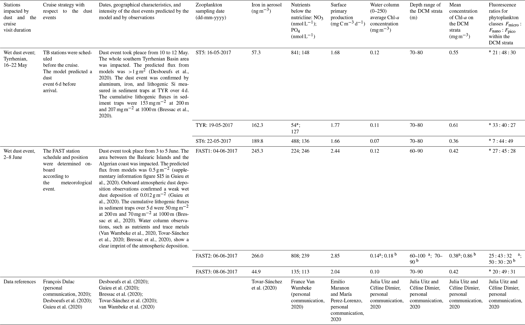
Table 2 Overview of the main characteristics of the wet dust events occurring during PEACETIME. Zooplankton sampling was carried out very close to a CTD cast at all stations except FAST2; at FAST2, sampling was undertaken between two casts: 9 h after the first cast ^a and 16 h before the second cast ^b. “^*” denotes that the value was measured on 17 May 2017. DCM refers to deep chlorophyll maximum.

2.2 Ancillary data on dust deposition events occurring during the PEACETIME survey

Guieu et al. (2020) detailed how they used three regional dust transport models to identify major dust events during the PEACETIME cruise. Two major wet dust events occurred during the study period (Table 2). The first event concerned the whole southern Tyrrhenian Basin, had a predicted flux of >1 g  m⁻² (Desboeufs et al., 2020), and started on May 10, several days before the arrival of the vessel in this area. The dust event was confirmed by aluminum, iron, and lithogenic Si measured in sediment traps at TYR station 6 to 9 d after the event and had a cumulative (4 d) lithogenic flux of 153 mg m⁻² at 200 m and 207 mg m⁻² at 1000 m (Bressac et al., 2020). The second event was located in the area between the Balearic Islands and the Algerian coast, occurred from 3 to 5 June, and had a predicted flux of 0.5 g m⁻² (Cécile Guieu, personal communication, 2020) after the arrival of the vessel in this area (FAST station). The dust event was confirmed by onboard atmospheric dust deposition samples (Desboeufs et al., 2020); water column observations, such as nutrients and trace metals, (Tovar-Sánchez et al., 2020); and tracers of dust deposition in sediment traps that had a cumulative (5 d) lithogenic flux of 50 mg m⁻² at 200 m and 70 mg m⁻² at 1000 m (Bressac et al., 2020). The lithogenic flux values at TYR and FAST are likely underestimated: considering that traps were placed with a time delay of 6 and 1 d following the dust event, the reported values could represent only a fraction of the total fluxes. The highest aerosol mass concentrations (around 25 µg m⁻³) with the highest iron content (245 ng m⁻³) were measured at FAST between 1 and 5 June, and the highest trace metal concentrations in the surface micro-layer were measured on 4 June (Co concentration of 773.6 pM, Cu concentration of 20.1 nM, Fe concentration of 1433.3 nM, and Pb concentration of 1294.7 pM; Tovar-Sánchez et al., 2020). The chemical composition of rain samples at FAST confirmed the wet deposition of dust that reached a total particulate flux of 0.012 g m⁻² (Fu et al., 2020). The Ionian Basin was the only southern area not impacted by dust deposition during the PEACETIME cruise; therefore, the results obtained at the long-duration ION station are considered (for comparison) to be results from an area that was not recently impacted.

2.3 Zooplankton sampling and sample processing

A total of 16 zooplankton samples were collected at 12 stations (Table 1) using a Bongo frame (double net ring of 60 cm mouth diameter) equipped with nets with a respective 100 and 200 µm mesh size (referred to as N₁₀₀ and N₂₀₀ in the following, respectively) mounted with filtering cod ends. At all sampling stations, the Bongo frame was vertically towed from a depth of 300 m to the surface at a constant speed of 1 ms⁻¹. The sample volume was estimated based on the ring diameter and the towed cable length. The sampling was mostly performed during the morning, except at ST7, ST9, and TYR, and night tows were also performed for the long-duration stations FAST and ION. The samples were preserved in 4 % borax-buffered formalin immediately after the net was hauled back onto the deck.

The samples were processed using a FlowCAM (Yokogawa Fluid Imaging Technologies Inc. Series VS-IV, benchtop model) (Sieracki et al., 1998) and a ZOOSCAN (Gorsky et al., 2010). One of the goals of this study was to achieve the determination of the complete size structure of the zooplankton community by combining plankton nets with different mesh sizes as well as different analysis techniques (FlowCAM and ZOOSCAN) in order to optimize the observed size spectrum. The formalin-preserved samples were rinsed with tap water to remove the formalin. For net N₁₀₀, the sample was then split into three size fractions: <200 µm (referred to as N₁₀₀F_<200 in the following), 200–1000 µm (referred to as N₁₀₀F_200∕1000 in the following), and >1000 µm (referred to as N₁₀₀F_>1000 in the following). For net N₂₀₀, the sample was split into two size fractions: <1000 µm (referred to as N₂₀₀F_<1000 in the following) and >1000 µm (referred to as N₂₀₀F_>1000 in the following).

To determine the complete size spectrum, different combinations of size fractions from the two nets and the two analytical techniques were tested using a two-way ANOVA. Taking the two mesh sizes (N₁₀₀ and N₂₀₀) into account, the limits of the size spectrum were defined from the N₁₀₀F_<200 fraction for the lower limit and from the N₂₀₀F_>1000 fraction for the upper limit. Considering that our FlowCAM does not detect particles larger than 1200 µm equivalent spherical diameter (ESD) and our ZOOSCAN does not detect particles smaller than 300 µm ESD, N₁₀₀F_<200 was analyzed by FlowCAM and N₂₀₀F_>1000 was analyzed by ZOOSCAN. The intermediate size fractions N₁₀₀F_200∕1000 and N₂₀₀F_<1000 were analyzed with both ZOOSCAN and FlowCAM. These analyses delivered abundance and biomass values for successive ESD size classes: <200 µm (referred to as C_<200), 200–300 µm (referred to as C_200−300), 300–500 µm (referred to as C_300−500), 500–1000 µm (referred to as C_500−1000), 1000–2000 µm (referred to as C_1000−2000), and >2000 µm (referred to as C_200−300). The challenge was to choose the best net–analysis technique combination for the intermediate size fractions (C_200−300, C_300−500, and C_500−1000). The abundance of each class for the two nets and the two treatments was statistically compared. Parts of the spectrum corresponding to the C_200−300 and C_300−500 fractions from N₁₀₀ measured with FlowCAM and to the C_500−1000 fraction from N₂₀₀ measured with the ZOOSCAN have significantly higher abundances than other net–analysis technique combinations (P<0.000). Consequently, we combined data from N₁₀₀F_<200 and N₁₀₀F_200−1000 measured with FlowCAM to compute ESD size classes <500 µm (Fig. 2a), and we combined data from N₂₀₀F_<1000 and N₂₀₀F_>1000 measured with ZOOSCAN to compute ESD size classes >500 µm (see Fig. 2b). The combination of these data enabled us to compute the final size spectrum (Fig. 2c) that was used to estimate abundance, biomass, and metabolic rates for each ESD size class as well as for the whole sample (sum of all of the size classes) and for the total mesozooplankton (sum of the size classes C_200−300, C_300−500, C_500−1000, and C_1000−2000).

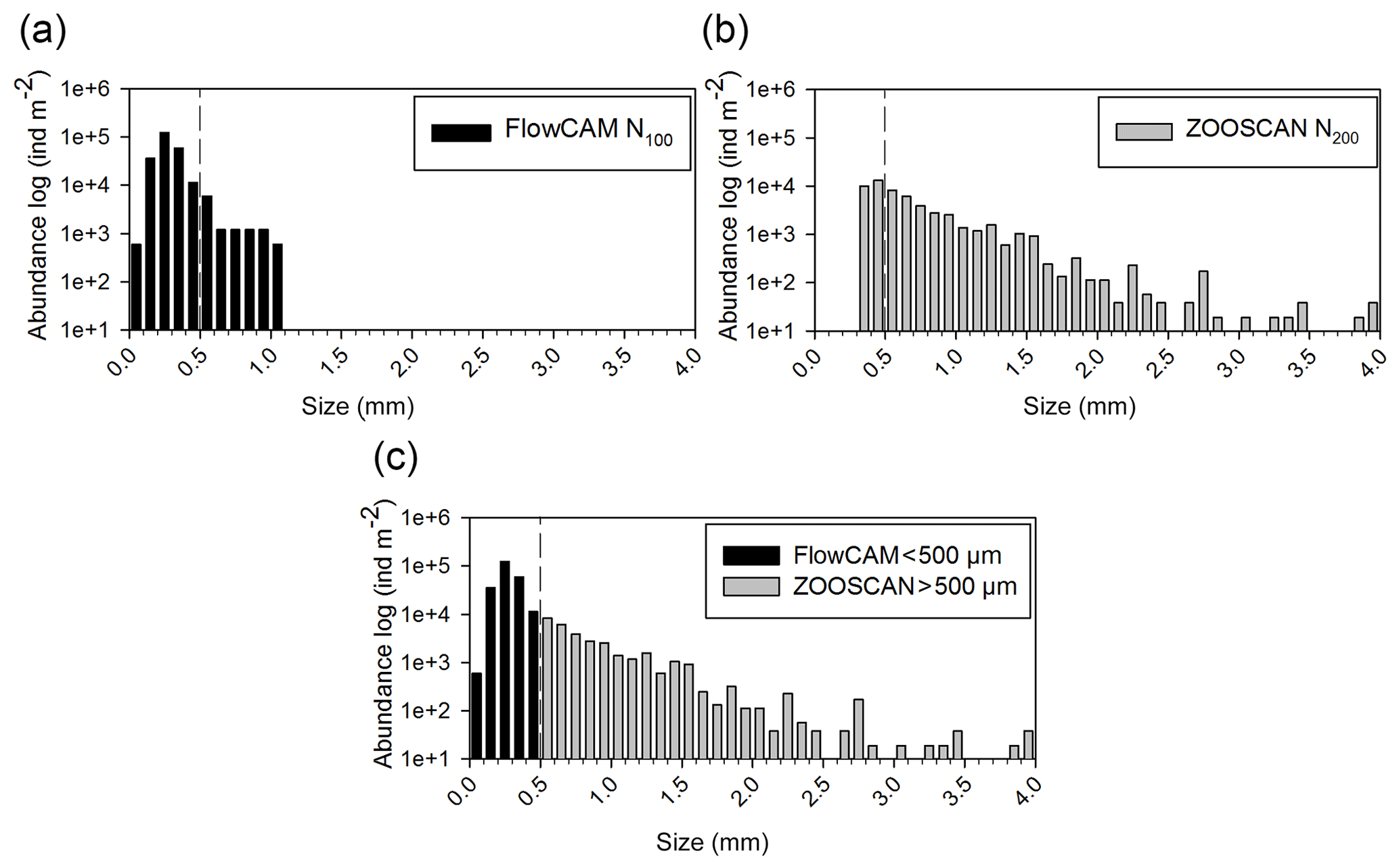
Figure 2 Size spectrum of ION1 (as an example) obtained by (a) FlowCAM (N₁₀₀), (b) ZOOSCAN (N₂₀₀), and (c) a combination of FlowCAM (N₁₀₀ counting only zooplankton smaller than 500 µm ESD) and ZOOSCAN (N₂₀₀ counting only zooplankton bigger than 500 µm ESD).

For the FlowCAM analyses, the sample was concentrated in a given water volume. An aliquot of each sample was then analyzed using FlowCAM in auto-image mode. For the N₁₀₀F_<200 fraction, a 4× magnification and a 300 µm field of view (FOV) flow cell were used, and the analysis was carried out up to 3000 counted particles. For the N₁₀₀F_200−1000 fraction a 2× magnification and 800 µm FOV flow cell were used, and the analysis was carried out up to 1500 counted particles.

The digitalized images were analyzed using the VisualSpeadsheet^® software and were manually classified into taxonomic categories. The living organism groups considered for the FlowCAM data were copepods, nauplii, crustaceans, appendicularians, gelatinous, chaetognaths, and other diverse zooplankton groups (such as Polychaeta and Ostracods). Non-organism particles were classified as detritus, and duplicates and bubbles were deleted.

To calculate the number of particles in the sample, the following equation was used:

$$\begin{array}{}\text{(1)}& A={\displaystyle \frac{p_{\mathrm{a}}\times V_{\mathrm{c}}}{V_{\mathrm{a}}\times V_{\mathrm{s}}}},\end{array}$$

where A is the abundance (individuals m⁻³), P_a is the number of particles in the analyzed aliquot, V_c is the given volume in the concentrated sample, V_a is the volume of the analyzed aliquot (m³), and V_s is the volume of sea water sampled by the zooplankton net (m³).

For the ZOOSCAN analyses, the sample was homogenized and split using a Motoda box until a minimum of 1000 particles were obtained. For the digitalization, the subsample was then placed onto the glass slide of the ZOOSCAN, and the organisms were manually separated using a wooden spike to avoid overlapping. After scanning, the images were processed with ZOOPROCESS (version 7.32) using the Image J image analysis software (Grosjean et al.,2004; Gorsky et al., 2010). Particles were automatically classified into taxonomic categories using the Plankton Identifier software (http://www.obs-vlfr.fr/~gaspari/Plankton_Identifier/index.php, last access: 27 October 2020). The classification was then manually verified to ensure that every vignette was in the correct category. The living groups of organisms considered for the ZOOSCAN were copepods, nauplii, crustaceans, appendicularians, gelatinous, chaetognaths, and diverse zooplankton (such as Polychaeta and Ostracods). Non-organism particles were classified as detritus, and blurs and bubbles were deleted.

2.4 Normalized biomass size spectrum

The size spectra were computed for each station using combined FlowCAM and ZOOSCAN data, following Suthers et al. (2006). The data were first classified into 0.1 mm ESD size categories from 0.2 to 2.0 mm. The zooplankton biovolume (mm³) was estimated for each category using the following equation:

$$\begin{array}{}\text{(2)}& \mathrm{biovolume}={\displaystyle \frac{\mathrm{1}}{\mathrm{6}}}\times \mathit{\pi }\times (\mathrm{ESD}{)}^{\mathrm{3}},\end{array}$$

with ESD expressed in millimeters. The x axis of the normalized biomass size spectrum (NBSS) was calculated by dividing the biovolume by the abundance of each category and was transformed into Log10. For the y axis, the biovolume of each category was divided by the difference in biovolume between two consecutive categories and was transformed into Log10. The NBSS slope and intercept were determined using a linear regression model. The slope of the NBSS reflects the balance between small and large individuals, with a steeper slope corresponding to a higher proportion of small individuals (bottom-up control) and a flatter slope corresponding to a higher proportion of large individuals (top-down control) (Donoso et al., 2017; Naito et al., 2019).

2.5 Zooplankton carbon demand, respiration, and excretion rates

The zooplankton carbon demand (ZCD, in mg C m⁻³ d⁻¹) was computed based on estimates of biomass from ZOOSCAN and FlowCAM samples and on estimates of the growth rate:

$$\begin{array}{}\text{(3)}& \mathrm{ZCD}=\mathrm{ration}\times B_{\mathrm{zoo}},\end{array}$$

where B_zoo is the biomass of zooplankton (in mg C m⁻³), which is calculated using the area–weight relationships from Lehette and Hernández-León (2009) and converted to carbon assuming that carbon represents 40 % of the total body dry weight (Omori and Ikeda, 1984). The ration (d⁻¹) is defined as the amount of food consumed per unit of biomass per day, and it is calculated as follows:

$$\begin{array}{}\text{(4)}& \mathrm{ration}=g_z+{\displaystyle \frac{r}{A}},\end{array}$$

where g_z is the growth rate, r is the weight-specific respiration, and A is the assimilation efficiency. g_z was calculated following Zhou et al. (2010):

$$\begin{array}{}\text{(5)}& g_z(w,T,\mathrm{Ca})=\mathrm{0.033}\left({\displaystyle \frac{\mathrm{Ca}}{\mathrm{Ca}+\mathrm{205}{e}^{-\mathrm{0.125}T}}}\right)e^{\mathrm{0.09}T}{w}^{-\mathrm{0.06}}\end{array}$$

and is a function of sea water temperature (T, ^∘C); food availability (Ca, mg C m⁻³), which is estimated from Chl a; and the weight of individuals (w, mg C). Here, we consider that the food is phytoplankton, following Calbet et al. (1996). Following Alcaraz et al. (2007) and Nival et al. (1975), values of r and A were 0.16 d⁻¹ and 0.7, respectively. ZCD was compared to the phytoplankton stock (converted to carbon assuming a C / Chl-a ratio of 50 / 1) and to primary production in order to estimate the potential clearance of phytoplankton by zooplankton.

Ammonium and phosphorus excretion and oxygen consumption rates were estimated using the multiple regression model by Ikeda et al. (1985) with carbon body weight and temperature as independent variables:

$$\begin{array}{}\text{(6)}& \ln y=a_{\mathrm{0}}+a_{\mathrm{1}}\ln x_{\mathrm{1}}+a_{\mathrm{2}}{x}_{\mathrm{2}},\end{array}$$

where lny represent the ammonium excretion, phosphorus excretion, or oxygen consumption; α₀, α₁, and α₂ are constants (see Ikeda et al., 1985); x₁ is the body mass (dry weight, carbon, nitrogen, or phosphorus weight); and x₂ is the habitat temperature (^∘C).

The contribution from zooplankton to nutrient regeneration was estimated using the values of primary production and was converted to nitrogen and phosphorus requirement using the Redfield ratio. Respiration was converted to respiratory carbon loss assuming a respiratory quotient for zooplankton of 0.97, following Ikeda et al. (2000), and was used as the carbon requirement for zooplankton metabolism.

2.6 Data analysis

Spatial patterns of the environmental variables were explored using a principal component analysis (PCA). We considered temperature, salinity, dissolved oxygen, and Chl-a values from a fluorescence sensor coupled to a CTD, using the mean values of the layer from 0 to 300 m as well as the estimated MLD. The data were normalized prior to the analyses, which were performed using PRIMER v7 software (Anderson et al., 2008).

Differences in zooplankton abundance and biomass between size classes and areas were tested using a two-way ANOVA. A one-way ANOVA with a Scheffé post hoc analysis was applied to compare mean values between areas for total zooplankton and within each size class. Data from prior analyses were log transformed and tested for homogeneity. Dunnett's test was used in case of inhomogeneity. Potential associations between univariate zooplankton and environmental data were tested using Spearman's rank correlations. These analyses were performed with Statistica 7 Software. The 100 µm sample from station TYR was discarded from these analyses due to the poor preservation state of the sample.

In order to study the spatial patterns of zooplankton communities, a taxonomic group–station matrix was created using the abundance values and was square root transformed to estimate station similarity using Bray–Curtis similarity. The similarity matrix was then ordinated using nonmetric multidimensional scaling (NMDS). The contributions of significant taxa to the similarity or dissimilarity between stations and areas were tested using SIMPER. The BIOENV algorithm was then used to select the environmental variables that best explained the spatial pattern observed for the zooplankton communities. A PERMANOVA was utilized to test the differences between areas based on environmental or zooplankton multivariate data. All of these analyses were performed using PRIMER v7 software (Anderson et al., 2008).

The relationships between the biological and the environmental variables were also studied by coupling multivariate analyses of two datasets. The first dataset featured the abundances of all the zooplankton taxa identified from the 200 µm net samples and the second dataset recorded environmental variables (the same as for the PCA analysis). A factorial correspondence analysis (FCA) and a principal component analysis (PCA) were performed on these two datasets, respectively. The results of the two analyses were then associated using a co-inertia analysis (Doledec and Chessel, 1994) that was performed using ADE-4 software (Thioulouse et al., 1997). Prior to the analyses, the data were log transformed to tend towards the normality of the distributions.

Rank frequency diagrams (RFD) were created using the data from N₂₀₀ in order to visualize differences in taxonomic composition between the samples. To improve the interpretation of the RFDs, we first used a method derived from Saeedghalati et al. (2017) based on the ordination of the normalized rank abundance distribution. A rank abundance matrix was created in which the data were standardized by the total abundance. Resemblance was measured with Bray–Curtis similarity, and a cluster was created using the complete linkage criterion. Second, a rank abundance distribution index was estimated following Mouillot and Lepretre (2000). The RFD for each station was separated into two portions: first the ranks with relative abundance <0.5 % were discarded (rare taxa, between 0 % and 30 % of the taxa according to all stations; by taking <1 % we would discard between 18 % and 49 % of the taxa) and then the two parts were fitted with a linear regressions. One part comprised the four highest ranks (see Mouillot and Lepretre, 2000 for the justification), and the remaining portion comprised the following ranks (between 15 and 23 taxa, depending on the station). The slope for both the upper and lower RFD portions was calculated (p₁ and p₂, respectively), and the p₁∕p₂ ratios were then estimated to quantify the differences between the RFDs of all of the stations.

3 Results

3.1 Spatial patterns of environmental variables

The principle component analysis (PCA) on environmental data explains 90.3 % of the total variance on the first two axes and delivers three clusters of oceanographic areas plus two distinct stations (Fig. 3). The first axis (62 % of the variance) is mostly influenced by temperature and dissolved oxygen, as shown by their high correlations with the scores of the sampling points on this axis (r=0.95 with p=0.000 and r=0.92 with p=0.000, respectively), whereas the second axis (28.3 %) is mostly influenced by MLD ($r=-\mathrm{0.75}$, p=0.01), salinity ($r=-\mathrm{0.75}$, p=0.001), and Chl-a ($r=-\mathrm{0.57}$, p=0.022; Table S1 in the Supplement).

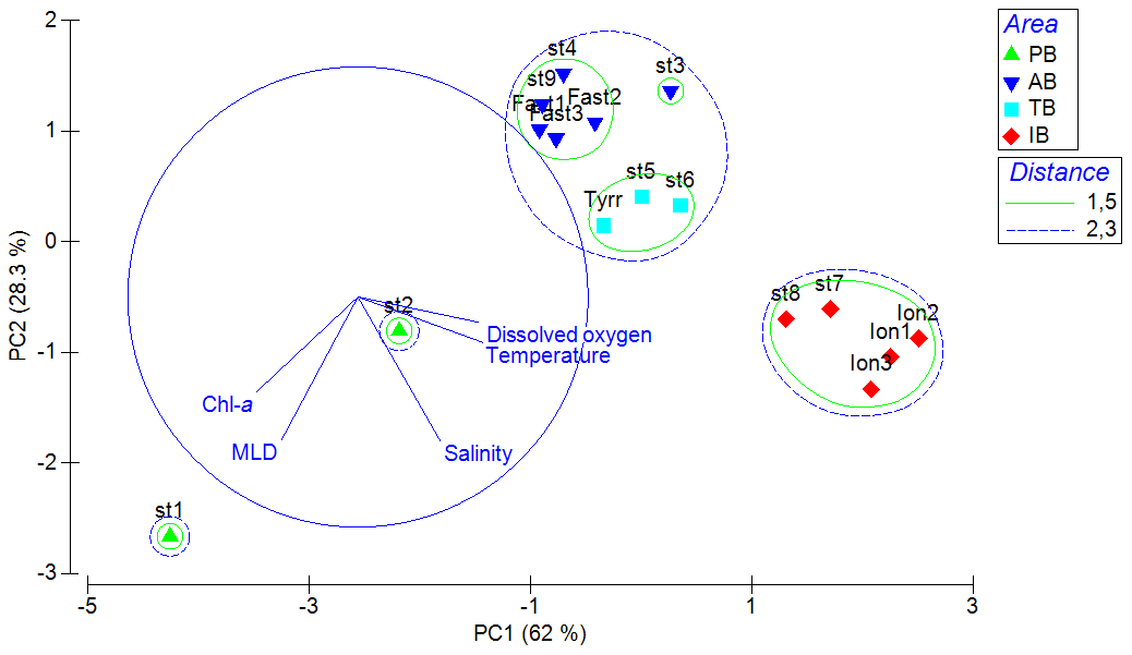
Figure 3 Principal component analysis (PCA) ordination of five environmental indicators: mixing layer depth (MLD), integrated values of the Chl-a concentration, and mean values in the upper $\mathrm{0}--\mathrm{300}$ m for temperature, salinity, and dissolved oxygen. AB refers to the Algerian Basin, PB refers to the Provencal Basin, TB refers to the Tyrrhenian Basin, and IB refers to the Ionian Basin.

The cluster of western stations in the Algerian Basin (AB) includes ST3, ST4, ST9, and FAST, which are characterized by low temperature, salinity, and MLD values. The cluster located in the Tyrrhenian Basin (TB) comprises ST5, ST6, and TYR and is very close to the first group but with lower Chl-a concentrations and higher temperature and salinity values. Eastern stations (ST7, ST8, and ION) located in the Ionian Basin (IB) are characterized by the highest temperature and salinity values and the lowest dissolved oxygen concentrations found during the survey. ST1 and ST2 in the Provencal Basin (PB) do not cluster with any of the other stations due to the deeper MLD and higher Chl-a concentrations.

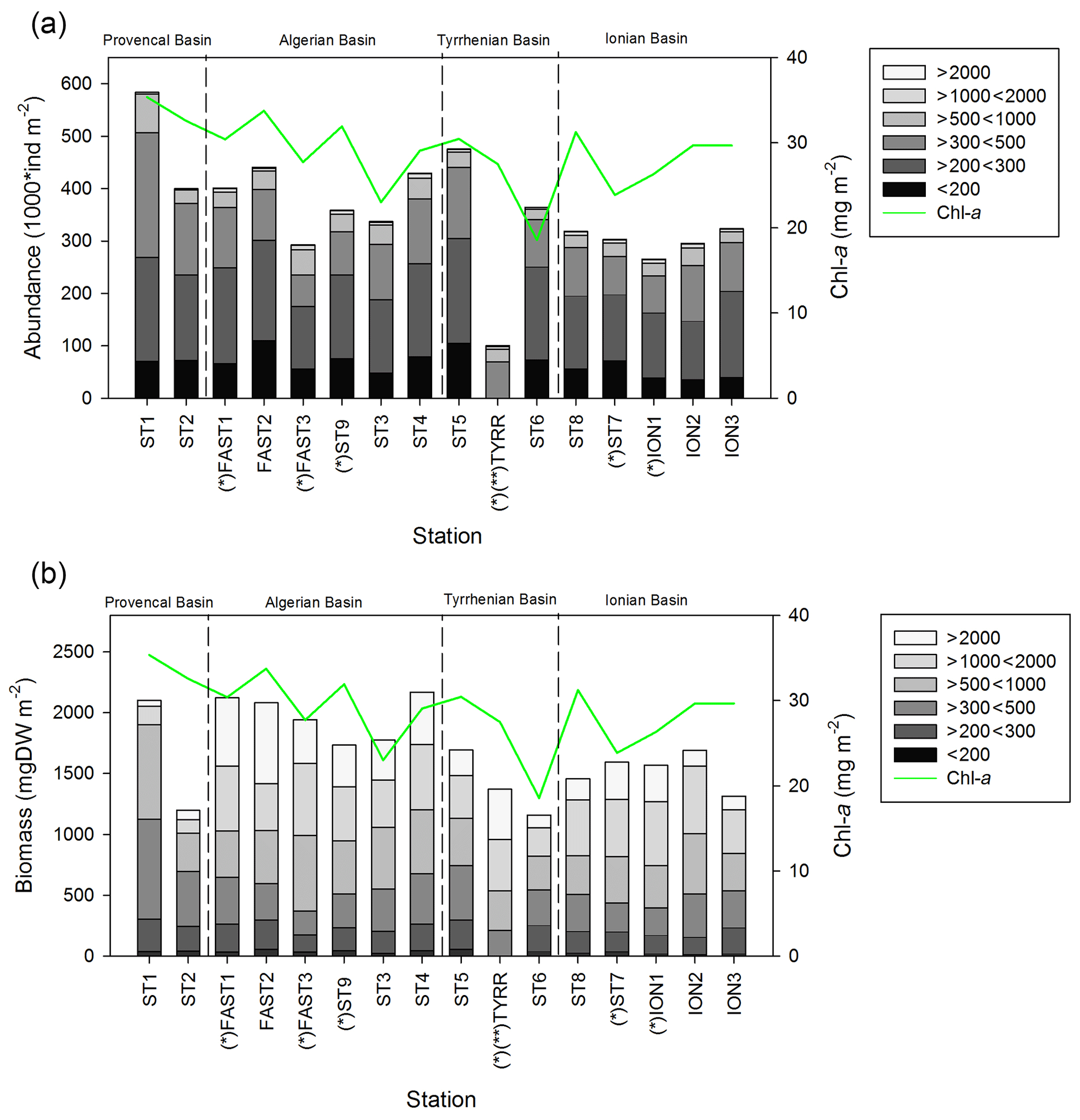
Figure 4 Values of zooplankton abundance (a) and biomass (b) cumulated by ESD size classes across different stations of the PEACETIME cruise. The green line shows the integrated Chl-a concentrations, “^*” denotes stations sampled during the night, and “${}^{**}$” denotes that only the abundance and biomass values above 300 µm are presented for TYR.

3.2 Spatial patterns of zooplankton structure

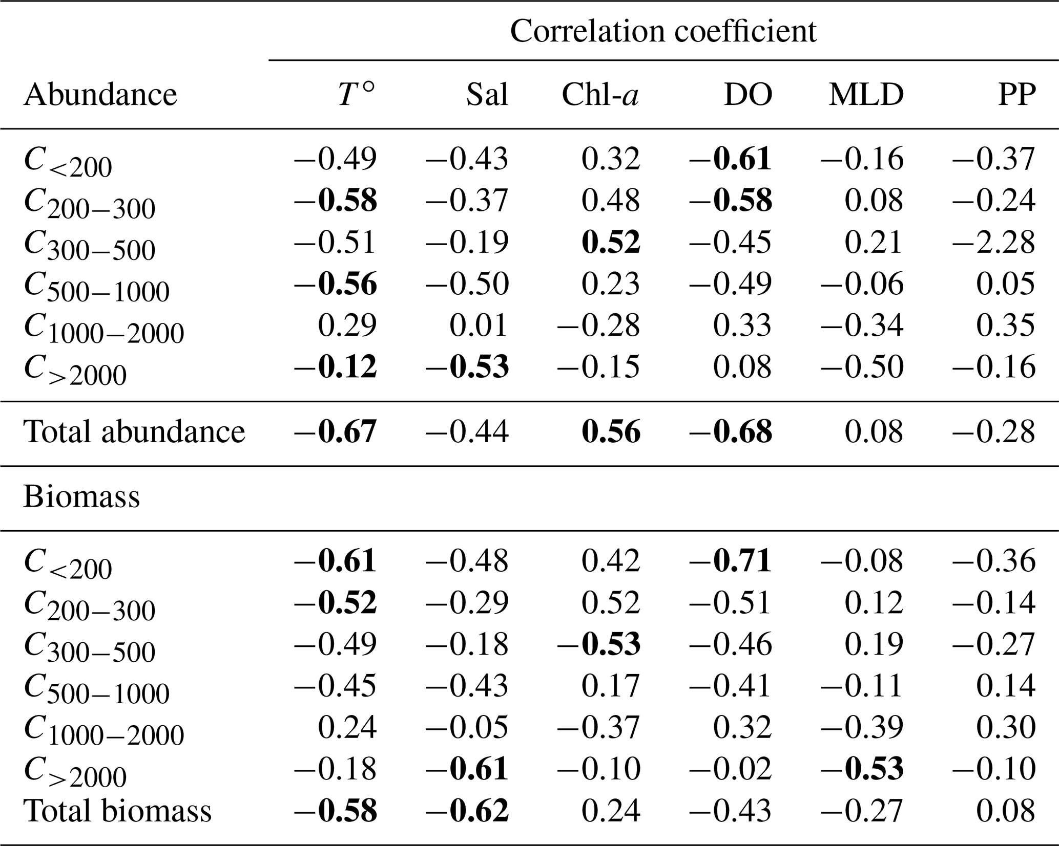
Zooplankton abundance (Fig. 4a) during the PEACETIME cruise ranges between 265×10³ and 583×10³ individuals m⁻², with an average of $\mathrm{372}\times {\mathrm{10}}^{\mathrm{3}}\pm \mathrm{84}\times {\mathrm{10}}^{\mathrm{3}}$ individuals m⁻², and zooplankton biomass (Fig. 4b) ranges from 1160 to 2170 mg DW m⁻², with an average of 1707±333 mg DW m⁻². The highest abundances are found in PB and AB, and the highest biomass is found in AB. The averaged total biomass in PB is lower than in AB due to the very low contribution of the C_1000−2000 and C_>2000 size classes, but the size classes from C_<200 to C_500−1000 present higher biomass values than in AB. In TB, the total biomass values decrease between ST4 and ST6, with the latter presenting the lowest biomass value of the whole survey. Note that the biomass values at TYR are only obtained for the size classes above 500 µm ESD, and the corresponding abundance value is comparable to those obtained at ST5 and ST6 for these larger size classes. In IB, total biomass and abundance are lower than at AB and have low variability between stations. The detritus estimated by FlowCAM and ZOOSCAN for all analyzed classes represents between 14.6 % and 39.1 % of the total biomass. The C_200−300 ESD size class has the highest average contribution (42.9 %) to the total zooplankton abundance, followed by C_300−500 (28.5 %), C_<200 (17.8 %), C_500−1000 (8,9 %), C_1000−2000 (1.7 %), and C_>2000 (0.22 %). In terms of biomass, C_500−1000 has the highest average contribution (25.3 %), followed by the C_1000−2000 (23.8 %), C_300−500 (21.3 %), C_>2000 (15.5 %), C_200−300 (11 %, 9 %), and C_<200 µm (2.1 %) fractions. There is no correlation between the total zooplankton abundance or biomass and the integrated Chl-a, but the C_300−500 biomass is negatively correlated with Chl-a ($r=-\mathrm{0.52}$, p=0.044). The total abundance is negatively correlated with temperature ($r=-\mathrm{0.67}$, p=0.006; Table 3).

Table 3 Table summarizing the Spearman's rank correlations. T^∘ represents temperature, Sal represents salinity, Chl-a represents chlorophyll, MLD represents the mixing layer depth, and PP represents primary production. Bold characters indicate a significant Rs value (p<0.05).

Copepods are the most abundant taxonomic group at all stations (Fig. 5), representing 40 % to 79 % of the abundance and 32 % to 85 % of the total biomass. The abundance of zooplankton smaller than 300 µm is dominated by cyclopoid and calanoid copepodites. In N₂₀₀, 51 taxonomic groups are found, 34 of which are copepod genera. The adult stages of the copepod community are dominated by the following genera: Para/Clausocalanus spp. (28.7 %), Oithona spp. (13.7 %), Corycaeus spp. (6.2 %), Oncaea spp. (4.1 %), and undefined calanoid copepods (7.0 %). The most abundant non-copepod groups are appendicularians (5.1 %), ostracods (4.8 %), and chaetognaths (3.6 %). The highest contributions of copepods to abundance and biomass are found in PB; this proportion then tends to decrease southwards as the abundance and biomass of the other groups such as chaetognaths and gelatinous zooplankton increase. The ratio between copepods with a length smaller than 1 mm and those larger than 1 mm (Fig. 5) ranges from 2.8 to 8.3 (5.1 on average), with the maximum mean values found in TB and the minimum values found in IB.

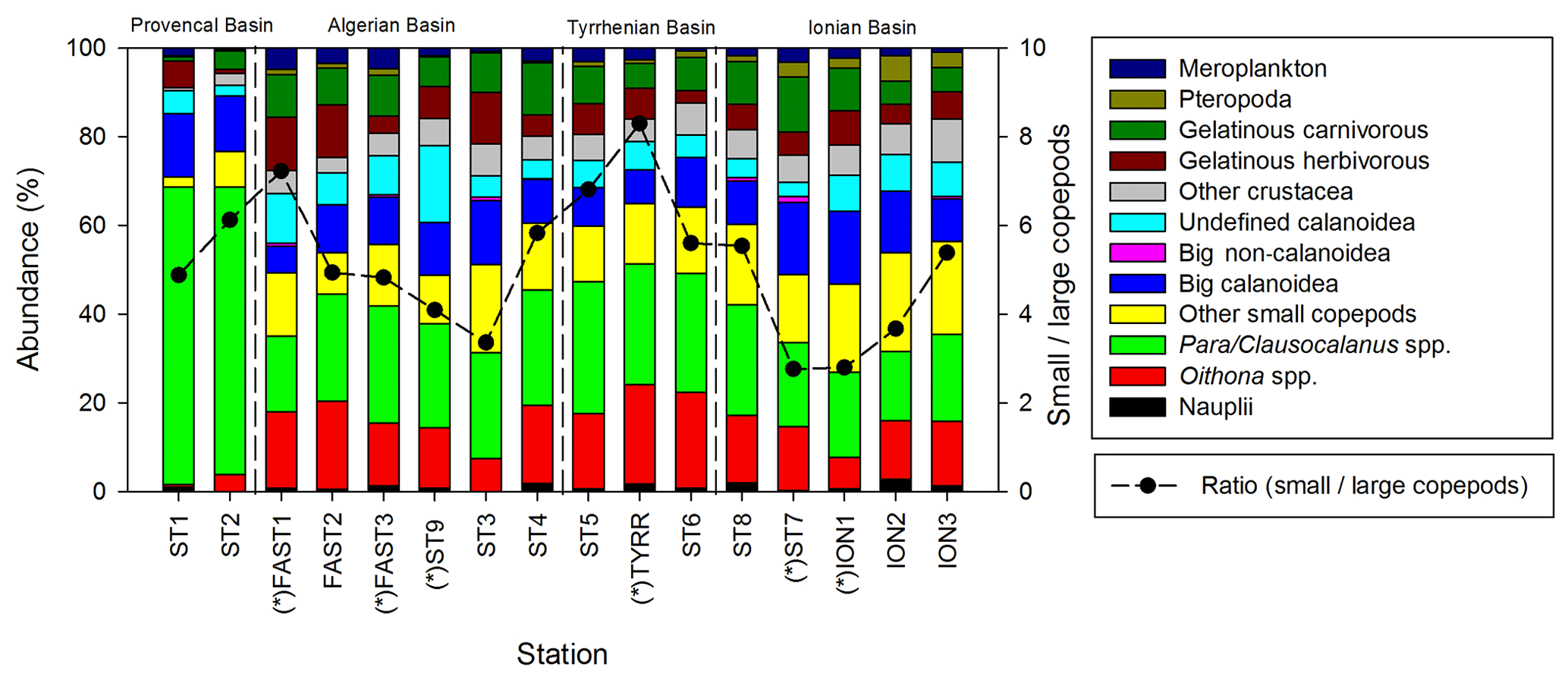
Figure 5 Spatial variation in taxonomic groups (bars) and the small (length <1 mm)/large (length >1 mm) copepod ratio (dashed line). “^*” denotes stations sampled during the night.

The two-way ANOVA shows that the PB is characterized by a significantly lower abundance and biomass in the upper size classes (1000–2000 and >2000 µm) compared with the other areas (p<0.05). One-way ANOVA results show that both total zooplankton and mesozooplankton present a significantly higher abundance in PB than in IB, whereas their total biomass was not significantly different between the areas (p>0.05). Significant differences in abundance and biomass between areas were found in the C_300−500, C_1000−2000, and C>2000 size classes and in the biomass for the C<200 class (P<0.05; Table 4 and Supplement Fig. S1).

Table 4 Results of the one-way ANOVA tests performed to test differences between areas (PB, AB, IB, and TB) with respect to the abundance and biomass data for the different zooplankton size classes, for total zooplankton (all size classes), and for mesozooplankton (ESD between 200 and 2000 µm) between the areas. Significant differences (p value <0.05) are marked in bold. “ns” denotes no significant difference. Italic F and p values mark where a Dunnett's test was used. In the post hoc analysis, the homogeneous groups with the lowest and highest values are noted using “a” and “b”, respectively. PB refers to Provencal Basin, AB refers to Algerian Basin, TB refers to Tyrrhenian Basin, and IB refers to Ionian Basin.

The NBSS is calculated for each station, as shown in Fig. 6, using ION1 as an example. During the PEACETIME survey, the NBSS slopes (Fig. 7) range from −0.60 to 1.27, with an average value of −0.80. The most negative slopes are found in PB, whereas the IB area has the fewest negative slopes. At the long-duration stations FAST and ION, strong variations in slope values appear depending on the sampling time, with the steeper slopes in the samples collected during the daytime indicating the higher contributions of small zooplankton compared with large zooplankton, which is potentially linked to the daily migration of larger forms to depths below 300 m.

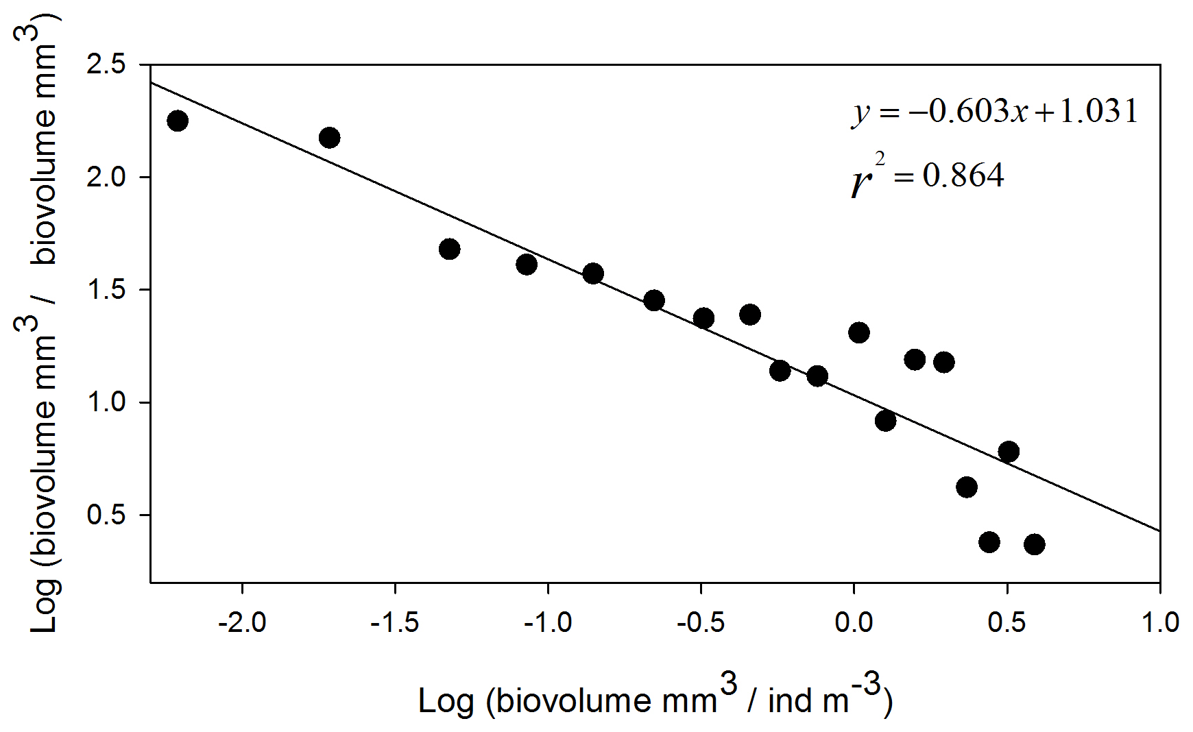
Figure 6 Normalized biomass size spectrum (NBSS) of mesozooplankton at ION1. Black dots show the normalized biomass values in the successive size classes, and the straight line represents the linear regression, giving the slope value.

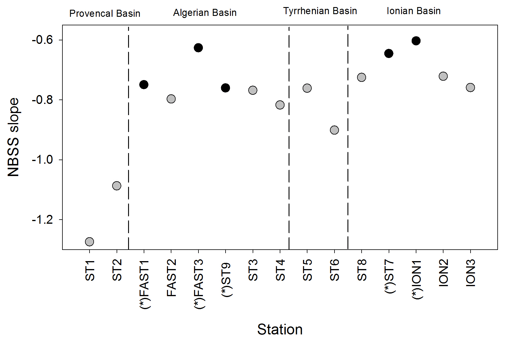
Figure 7 NBSS slope values of mesozooplankton obtained for all stations during the PEACETIME survey. Black dots represent night samples, and gray dots represent day samples.

The NMDS analysis (Fig. 8) on the mesozooplanktonic taxa abundances based on N₂₀₀ delivers a distribution pattern for the stations that is rather similar to that of the PCA on environmental variables. ST1 and ST2 in PB are the most dissimilar stations due to the higher abundance of copepods – especially the abundance of Para/Clausocalanus spp. at ST1, which is twice as high as at ST2 and between 5 and 13 times higher than the rest of the transect (Figs. 5, 8a). Similarly, the Centropages spp. abundance is 10 times higher at ST1 and ST2 than at other stations in the survey. In contrast, the abundances of Oithona spp. and Corycaeus spp. are 6 and 10 times lower at ST1 and ST2, respectively, than at other stations. The zooplankton community in AB is slightly different from those in TB and IB due to appendicularians and unidentified calanoid copepods being more abundant in AB and due to Haloptilus spp. being more abundant in TB and IB. Within TB and IB, the three sampling dates (ION1, ION2, and ION3) at ION form a unique cluster, whereas ST7 and ST8 are grouped with station TB in another cluster. This differentiation of ST7 and ST8 from the ION sampling dates in the NMDS analysis is mainly due to differences in the relative abundance of Mesocalanus spp. (more abundant), ostracods (less abundant), Clytemnestra spp. (absent in ION), and Pontellidae. (absent at ST7 and ST8).

Figure 8 NMDS analysis of the zooplankton taxa for all stations (a) excluding ST 1 and ST2. (b) A plot of the stations and the taxa correlated at >0.65 with the axes. The color of the stations represents the areas identified by the PCA in the environmental analysis (see Fig. 2). This analysis was performed on the zooplankton collected with the data from N₂₀₀. PB refers to Provencal Basin, AB refers to Algerian Basin, TB refers to Tyrrhenian Basin, and IB refers to Ionian Basin.

The SIMPER analysis shows that the lower average similarity between the stations (64.79 %) is mainly due to Para/Clausocalanus spp. in PB. The rest of the basins share a higher internal similarity: 78.43 %, 79.79 %, and 78.03 % for AB, TB, and IB, respectively. Another interesting point highlighted in the SIMPER analysis is the lower average dissimilarity between TB and stations ST7 and ST8 (20.25 %). This dissimilarity increases when the comparison is made between TB and the rest of the stations included in IB (29.04 %); this finding is in agreement with the NMDS analysis (Fig. 8) that related ST7 and ST8 to TB rather than to the stations in their basin.

3.3 Relationship between the environmental variables and the zooplankton community

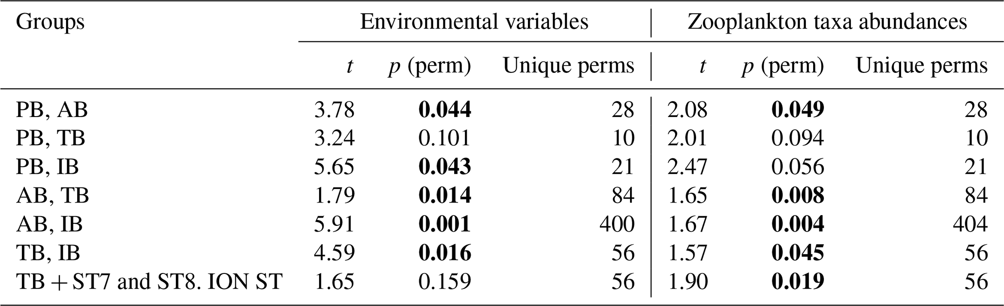
Results of the PERMANOVA analysis on the environmental variables and on the diversity of taxa are summarized in Table 5. Interestingly, based on the zooplankton diversity of TB and IB, their difference is more significant when ST7 and ST8 are removed from IB and placed in TB (based on the NMDS cluster, Fig. 8), whereas this is not the case when considering environmental variables (see Table 5). This suggests that the similarity between ST7 and ST8 and the TB stations is not linked to the environmental context.

Table 5 PERMANOVA analysis on the environmental variables and on zooplankton taxa abundances: pair-wise tests with unrestricted permutation of raw data (number of permutations: 999) were used for the comparison between the zones. Resemblance worksheets are based on Euclidean distance. Significant p values (p <0.05) are marked in bold.

The BIOENV results show that salinity and chlorophyll were the environmental variables that best explained the overall spatial distribution of the zooplankton community (BIOENV; Rs=0.657).

The first factorial plane of the co-inertia analysis (Fig. 9) explained 96 % of the total variance, with 79 % due to the first axis. For both spaces (“Environment” and “Zooplankton”), the IB stations on the first axis are associated with high temperature and salinity values and several zooplankton taxa (namely echinoderm larvae and some copepod taxa, e.g., Pontellidae, Rhincalanus spp., Haloptilus spp., and Phaena spp.) and are separated from the PB and AB stations correlated with higher chlorophyll concentrations and with some copepod taxa (mainly Pseudodiaptomus spp., Tortanus spp., and Pleuromamma spp.). On this axis, TB stations have an intermediate position, close to the coordinate zero. The second axis opposes northern (ST1 and ST2 in PB) and southern (AB) stations sampled in the western Mediterranean Basin. On this axis, PB stations are characterized by higher chlorophyll and salinity values and a deeper MLD compared with AB and by the association with Pseudodiaptomus spp., whereas southern AB stations are associated with the copepods Heterorhabdus spp., Labidocera spp., and Euterpina spp. As in the preceding multivariate analyses, we note that ST8 and ST9 from the IB tend to be closer to the TB stations than to the ION station on the first factorial plane, particularly in the “Zooplankton system”. The association between the environmental context and the zooplankton community is high with good correlation between the normalized scores of the stations (R²=0.844 and R²=0.820 for the x₁ and x₂ axes, respectively) and with the positions of the plots of these stations close to the equality lines (i.e., x₁ Zooplankton =x₁ Environment or x₂ Zooplankton =x₂ Environment).

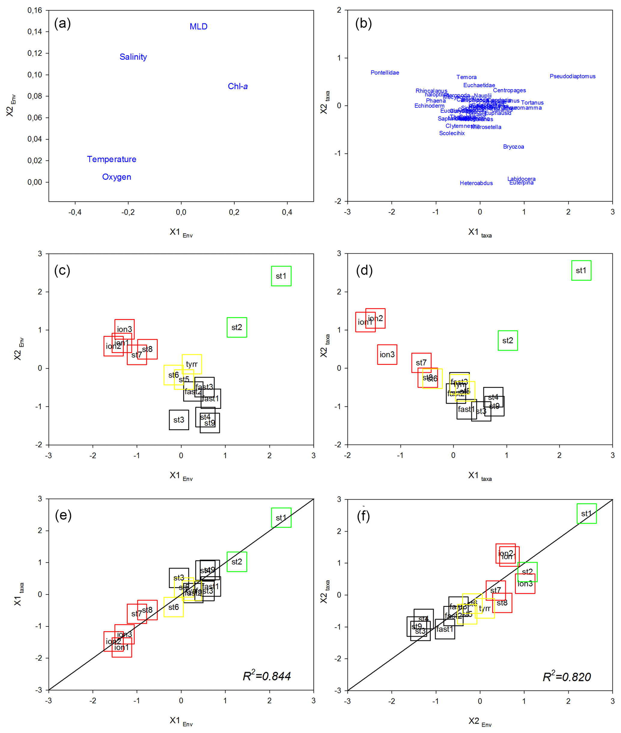
Figure 9 Co-inertia analysis. Ordination on the plans (1, 2) of the environmental variables (a) and the abundance of the zooplankton taxa (b). Ordination on the plans (1, 2) of the stations in the “Environment system” (c) and in the “Zooplankton system” as well as plots of the stations on the first (c) and second (d) axes of the two systems. Lines represent the equality between the coordinates on the two systems. Colored squares identify the different regions: green denotes PB, black denotes AB, yellow denotes TB, and red denotes IB.

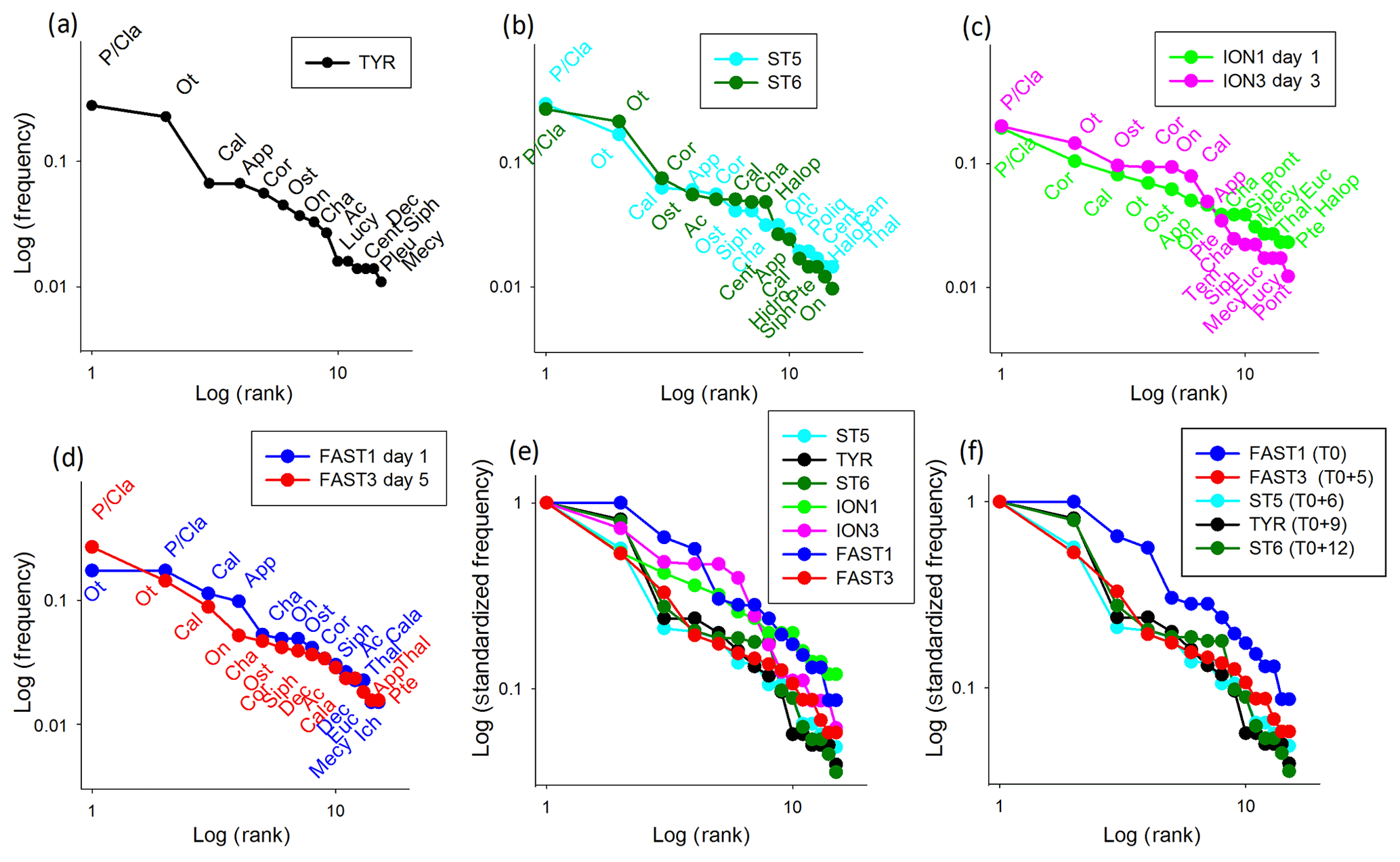
Figure 10 Rank frequency diagram at TYR (a), ST5 and ST6 (b), ION (c), FAST (d), and the Log-standardized frequency for all stations (e) and stations influenced by dust deposition (f). Ac denotes Acartia spp., Cal denotes calanoid copepods, Cala denotes Calanus spp., Cent denotes Centropages spp., Cor denotes Corycaeus spp., Euc denotes Eucalanus spp., Halop denotes Haloptilus spp., Luci denotes Lucicutia spp., Mecy denotes Mecynocera spp., On denotes Oncaea spp., Ot denotes Oithona spp., P∕Cla denotes Para/Clausocalanus spp., Pleu denotes Pleuromamma spp., Pont denotes Pontellidae, Tem denotes Temora spp., App denotes Appendicularia, Cha denotes Chaetognatha, Dec denotes decapods, Hydro denotes hydrozoans, Ich denotes ichtyoplankton, Ost denotes ostracods, Poly denotes Polychaeta, Pte denotes pteropods, Siph denotes siphonophores, and Thal denotes thaliaceans.

3.4 Zooplankton community changes linked to dust deposition events during the PEACETIME survey

The zooplankton community changes were analyzed using the variations in the RFDs between samplings. The RFDs for TYR, ST5, ST6, ION, and FAST are presented separately in Fig. 10a–d and are grouped in Fig. 10e and f. As only one sample was carried out at TYR, 9 d after a large dust deposition event in the southern Tyrrhenian Basin, the RFDs of ST5 and ST6 also sampled in TB (6 and 12 d after the dust event, respectively) are added for comparison (Fig. 10a, b). At all three TB stations, the RFDs are characterized by the high dominance of the filter-feeding zooplankton Para/Clausocalanus spp. and Oithona spp. in the first and second positions and a strong drop in abundance for the following ranked taxa (undefined calanoid copepods or Corycaeus spp.). Appendicularians drop from the fourth position at ST5 and TYR to the tenth position at ST6. The shapes of the RFDs change more between ST5 and TYR than between TYR and ST6. At ION, which was not impacted by dust deposition, the RFD shapes are similar for both sampling dates (ION1 and ION3), and the community is dominated by Para/Clausocalanus spp. (Fig. 10c). Corycaeus spp. changes from the second position to the fourth, calanoid copepods change from the third position to the sixth, and Oithona spp. changes from the fourth position to the second. Appendicularians occupy a very similar position in both RFDs (sixth and seventh rank at ION1 and ION3, respectively). At FAST, the taxonomic composition is dominated by copepods (Fig. 10d), but the rank order of the most dominant species changes between the two sampling dates (FAST1 and FAST3). Oithona spp. and Para/Clausocalanus spp. have the first and second ranks during FAST1, but this order is reversed during FAST 3. The third place on both days is occupied by calanoid copepods. Appendicularians present one of the most significant changes, with their rank dropping from fourth to fourteenth between the two dates. It is remarkable that the RFDs change from a convex shape at FAST1 to a more concave one at FAST2, which is influenced by the high dominance of Para/Clausocalanus spp. at the first rank (Fig. 10d). The comparison of the standardized RFDs for all of the stations (Fig. 10e) highlights that the greatest change in shape is visible at FAST, whereas it remains moderate at ION and negligible at TB. Figure 10f is similar to Fig. 10e, except without ION, in order to visualize changes in the zooplankton community composition at different time lags after a dust event. This will be commented on in more detail in Sect. 4. The RFDs for all stations are shown in Fig. S2 in the Supplement.

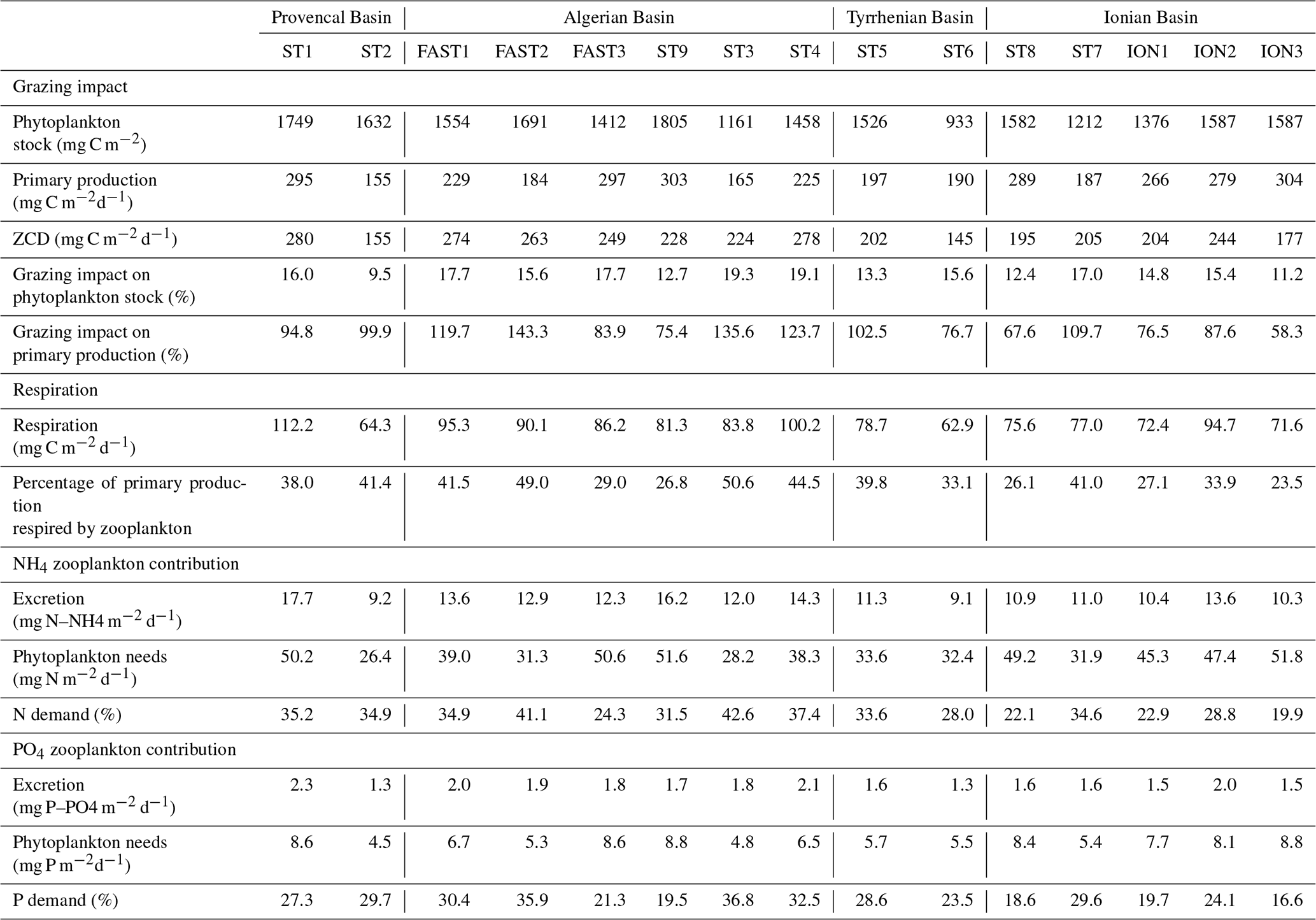
Table 6 Estimated grazing, respiration, and excretion rates of zooplankton based on allometric models (see Sect. 2) and their impact on the phytoplankton stock and production along the PEACETIME survey transect.

3.5 Estimated zooplankton carbon demand, grazing pressure, respiration, and excretion rates

Zooplankton carbon demand ZCD (Table 6) varies between 145.9 and 280.1 mg C m⁻² d⁻¹ at ST6 and FAST1, respectively. Assuming that phytoplankton is the major food source, zooplankton consumption potentially represents 15 % of the phytoplankton stock on average per day and 97 % of the primary production (see Table 6). ZCD follows the zooplankton biomass pattern with higher values in AB and lower values in TB, and it does not increase with primary production ($r=-\mathrm{0.18}$, p>0.05). The average respiration (mean of 83.1 mg C m⁻² d⁻¹ and range between 62.9 and 112.2 mg C m⁻² d⁻¹) corresponds to 36.4 % of the integrated primary production. Almost half of this zooplankton respiration is due to organisms smaller than 500 µm ESD. Mean ammonium excretion is 12.3 mg NH₄ m⁻² d⁻¹ (range between 9.1 and 17.7 mg NH₄ m⁻² d⁻¹), and mean phosphate excretion is 1.7 mg PO₄ m⁻² d⁻¹ (range between 1.3 and 2.3 PO₄ m⁻² d⁻¹). The potential contributions of excreted nitrogen and phosphorus to primary production are 31.5 % (range between 19.9 % and 42.6 %) and 26.3 % (range between 19.9 % and 42.6 %), respectively. Zooplankton size classes smaller than 500 µm ESD contribute 45 % and 47 % of the total ammonium and phosphate excretion, respectively. Estimated values for all zooplankton size classes for grazing, respiration, and excretion rates and for their impact on the phytoplankton stock and production along the PEACETIME survey transect are presented in Table S2 in the Supplement.

4 Discussion

4.1 Methodological concerns and the importance of the small zooplankton fraction

The methodology used in this study – combining two nets (N₁₀₀ and N₂₀₀) and two sample treatments (FlowCAM and ZOOSCAN) – enables us to deliver a more accurate mesozooplankton community size spectrum (200–2000 µm), although the C_<200 and C_>2000 size classes at the edges of the spectrum range remain undersampled and require different equipment for proper sampling (bottles and a larger mesh size net, respectively). The length / width ratio of mesozooplankton organisms is quite variable and ranges from 1 for nearly spherical organisms, such as nauplii or cladoceran, to more than 10 for long organisms, such as chaetognaths (Pearre, 1982) or some copepods like Macrosetella gracilis (Böttger-Schnack, 1989), with an average value of between 3 and 4 for copepods (Mauchline, 1998). If we consider that organisms with a length / width ratio of 6 caught by the 200 µm mesh size will present an ESD of at least 490 µm, it is consistent that this net quite correctly samples organisms with an ESD above 500 µm. For these organisms (>500 µm ESD), ZOOSCAN is the most appropriate tool to deliver the size spectrum. Similarly, the 100 µm mesh size net allows small organisms with a width just below 100 µm to pass through; however, most of them might have an ESD of up to 200 µm because the length / width ratio is mostly below 4 for these smaller sizes (Mauchline, 1998). Due to the threshold of ZOOSCAN at 300 µm ESD, FlowCAM is the best tool to process organisms in the fraction below 500 µm.

Several authors have already highlighted the limitation of the 200 µm mesh size with respect to catching small zooplankton individuals. Comparisons of different zooplankton nets' mesh sizes between 60 and 330 µm have systematically shown a decrease in plankton abundance with an increasing mesh size (Turner, 2004; Pasternak et al., 2008; Riccardi, 2010; Makabe et al., 2012; Altukhov et al., 2015). When the goal of the study is to achieve a full understanding of the complete mesozooplankton community structure and function, the size selectivity of the sampling nets is an important issue: clearly, a large fraction of organisms between 200 and 500 µm ESD is undersampled using a single 200 µm mesh size. Pasternak et al. (2008) reported that a 220 µm mesh can lose up to 98 % of the abundance of Oithona spp. and 80 % of copepodite stages of Calanus spp. Riccardi (2010) found that a classical 200 µm net catches only 11 % of the abundance and 54 % of the biomass compared with a 80 µm mesh size, which, in that study, led to differences in the observed species composition in the Venice Lagoon. During the PEACETIME survey, the small size classes (C_200−300 and C_300−500) of mesozooplankton have been optimally sampled using a 100 µm mesh size (N₁₀₀). Consequently, these size classes represent very large percentages of the total abundance (52.3 % and 34.8 %, respectively) and a significant contribution to the total biomass (14.5 % and 25.9 %, respectively). These reliable estimations have direct consequences for the estimated fluxes (see below).

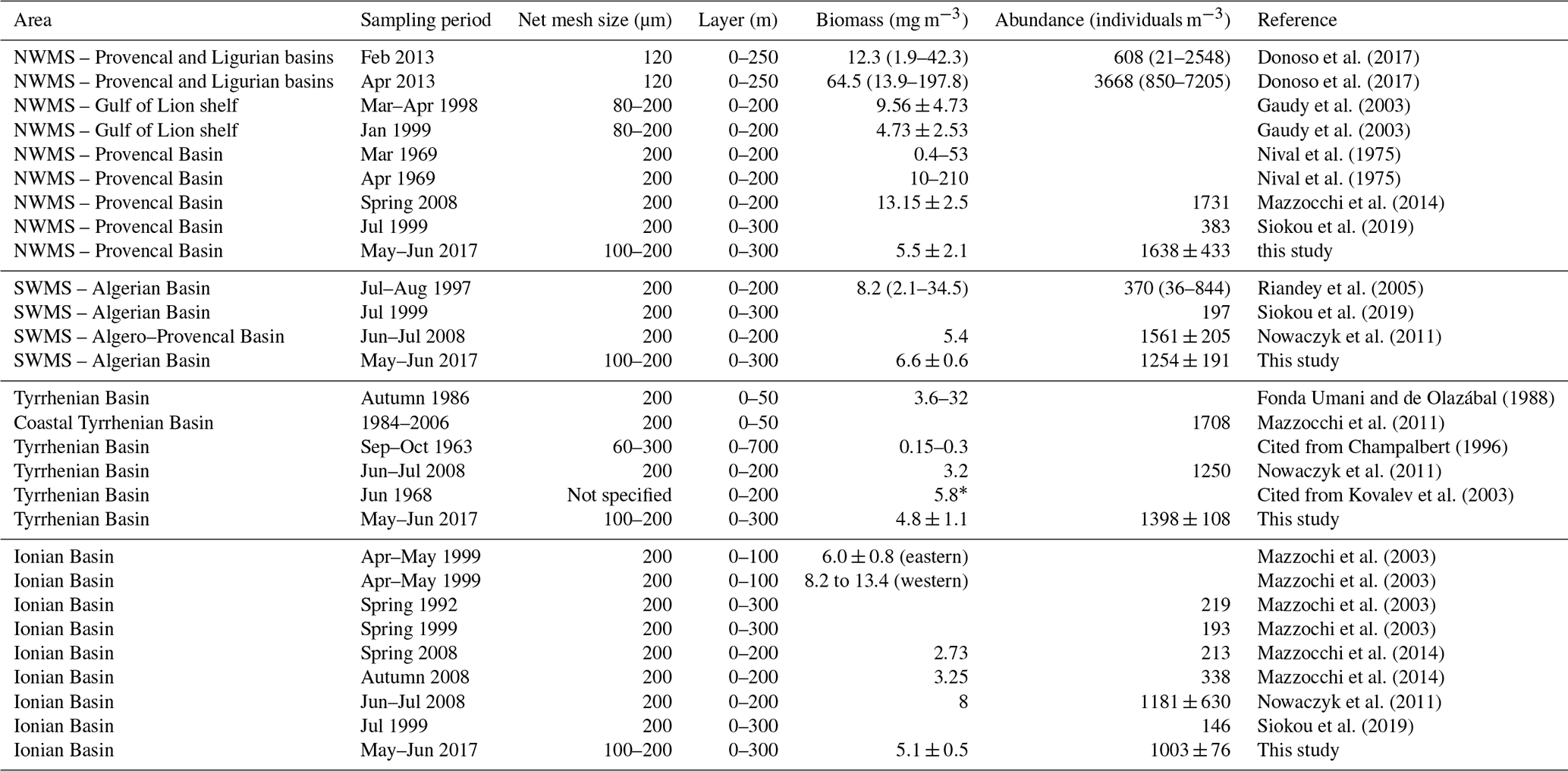
Table 7 Comparison of zooplankton biomass and abundance in different areas of the Mediterranean Sea. “*” denotes the wet weight. NWMS refers to the northwestern Mediterranean Sea, and SWMS refers to the southwestern Mediterranean Sea.

4.2 Differences in abundance, biomass, and zooplankton community structure in relation to regional environmental characteristics

A review of the most relevant information available on zooplankton biomass and abundance in different regions of the central and western Mediterranean Sea (Table 7) shows a wide range of variation that can be attributed to location, sampling seasons, and/or sampling methods (e.g., net mesh size and depth of tow). In general, the values from the PEACETIME survey are of the same order of magnitude as values from previous studies, although most of the other studies were performed with a 200 µm mesh size net and often over a shallower surface layer. However, during this post-bloom period, no clear regional patterns in abundance and biomass were found, unlike other descriptions showing a north–south and west–east decrease in zooplankton stocks (Dolan et al., 2002; Siokou-Frangou, 2004). In PB, Donoso et al. (2017) and Nival et al. (1975) highlighted a strong variability that is consistent with the strong gradient found between ST1 and ST2 during PEACETIME (see Fig. 4). In AB, abundance and biomass values obtained during the survey are similar to those recorded in late spring by Nowaczyk et al. (2011), whereas Riandey et al. (2005) found lower abundance and higher biomass values. However, the latter study focused on the high resolution of a mesoscale eddy, highlighting an important fine-scale variability in abundance and biomass values. For TB, the data are difficult to compare due to the different sampling conditions (net mesh size, depth of tow, and sampling season). In IB, all biomass values presented in Table 7 are of the same order of magnitude, although abundances found by Mazzocchi et al. (2003, 2014) are 3 times lower than those observed during PEACETIME, which is probably due to the high contribution of C_<200 and C_200−300 obtained with N₁₀₀ (see Fig. 4). In general, the better sampling of small size classes with N₁₀₀ should lead to higher abundance values. However, the comparison of data in Table 7 shows that the regional and temporal variability of these values partially masks this benefit.

In PEACETIME, clear regional differences are found both in terms of environmental variables and zooplankton taxonomic composition. ST1 and ST2 are clearly differentiated from all of the other stations by a deeper MLD, higher Chl-a concentrations, and a zooplankton community dominated by herbivorous copepods typical of the PB (e.g., Centropages, Para/Clausocalanus, and Acartia,), as mentioned by Gaudy et al. (2003) and Donoso et al. (2017), and characterized by a scarcity of thaliaceans which normally occur in ephemeral and aperiodic patches (Deibel and Paffenhöfer, 2009). AB and TB are very closely related to each other in terms of hydrological features and Chl-a, but they are slightly differentiated with respect to salinity and zooplankton taxonomy, probably because they are both strongly influenced by the Modified Atlantic Water (MAW) and its associated mesoscale features (Millot and Taupier-Letage, 2005). In AB, 17 d separated the sampling of ST3 and ST4 from that of ST9 and FAST; however, despite this time gap, they are very close in terms of hydrological features, Chl-a level, and zooplankton community structure. IB is clearly differentiated from these groups in terms of environmental parameters (see Fig. 3) due to a higher salinity and a lower Chl-a concentration; however, in terms of zooplankton community, the western Ionian stations (ST7 and ST8) present more analogy with TB than with the ION (see Fig. 8). During PEACETIME, ION appears to be clearly separated from ST7 and ST8 that are located further westwards by a north–south jet (ADCP and MVP observations, Leo Berline, personal communication, 2020), which might correspond to the “Mid-Mediterranean Jet” (Malanotte-Rizzoli et al., 2014, their Fig. 5). The location of ST7 and ST8 within the anticyclonic structures of the portion of the Modified Atlantic Water (MAW) flowing through the Strait of Sicily could explain their similarity to the TB stations in terms of zooplankton assemblages – as TB is directly influenced by the main part of the MAW flowing through the Sardinian Channel. Ayata et al. (2018) also classified the Tyrrhenian Basin as heterogeneous due to complex circulation patterns including transient hydrodynamic structures in the south, which could also explain the similarity of ST7 and ST8 to the TB stations in terms of zooplankton assemblages during PEACETIME. This area of the IB visited during PEACETIME certainly represents a transition area between the eastern and western Mediterranean basins (Siokou-Frangou et al., 2010; Mazzocchi et al., 2003).

These regional differences, highlighted both in terms of environmental characteristics and zooplankton taxa assemblages, are in agreement with the regionalization of the Mediterranean Basin by Ayata et al. (2018) based on historical biogeochemical, biological, and physical data of the epipelagic zone. For example, ST1 of PEACETIME, which is characterized by high Chl-a, high zooplankton abundance, and the dominance of small copepods, is clearly located in the “consensual Ligurian Sea Region” sensu Ayata et al. (2018), which has been identified as the most productive region of the Mediterranean due to intense deep convection events. Among the AB stations, ST3, ST4, and ST9 are clearly within the “consensual Algerian region” (Ayata et al., 2018), whereas FAST corresponds to the “western Algerian heterogeneous region”. Among the IB stations, ST7 and ST8 from the ION stations in terms of zooplankton communities and, to a lesser extent, environmental variables, also correspond to the distinction between the “consensual North Ionian” region and the western part of the “Ionian Sea region”, which is considered to be a heterogeneous region (Ayata et al., 2018).

4.3 Estimated zooplankton-mediated fluxes during the PEACETIME survey

By using allometric relationships relating zooplankton grazing and metabolic rates to size structure, zooplankton impacts (top-down vs. bottom-up impacts) on primary production have been investigated. We are aware that using constant conversion factors may limit the analysis of the spatial variation, as these factors may display temporal and geographical variations (Minutoli and Guglielmo, 2009). However, our sampling strategy based on a limited number of stations sampled did not enable us to consider temporal and spatial variations accurately, and our main goal was to roughly estimate the epipelagic zooplankton-mediated fluxes at the scale of the PEACETIME cruise.

Figure 11 Cluster analysis on rank frequency diagrams (a) and changing trends in the p₁∕p₂ ratio (b) on the stations impacted by wet dust deposition.

ZCD estimations show that zooplankton required 15 % of the daily phytoplankton stock, with narrow variations over the whole area (between 9.5 and 19.3), which is twice as low as the values estimated by Donoso et al. (2017) during the spring bloom in the northwestern Mediterranean Sea. However, estimated grazing rates are of the same order as the estimated primary production, which corresponds to the highest range of the values summarized by Siokou-Frangou et al. (2010) for the whole Mediterranean Sea (from 14 % to 100 %). Estimating ZCD on the basis of mesozooplankton alone certainly leads to an overestimation of its top-down impact on phytoplankton. In the Mediterranean Sea, primary production is consumed by a “multivorous web” including microbial and zooplankton components (Siokou-Frangou et al., 2010). Mesozooplankton simultaneously grazes on phytoplankton and heterotrophic prey, such as heterotrophic dinoflagellates (Sherr and Sherr, 2007) or ciliates (Dolan et al., 2002), and might be quite flexible in its feeding strategy depending on the composition and size of prey as well as the environmental variables such as turbulence (Kleppel, 1993; Yang en al., 2010). On the one hand, a large part of the primary production can be consumed by ciliates (Dolan and Marrasé et al., 1995), but, on the other hand, mesozooplankton can consume almost the entire ciliate production (Pitta et al., 2001; Pérez et al., 1997; Zervoudaki et al., 2007), which potentially explains the wide variations in the ciliate standing stock over the Mediterranean Sea (Dolan et al., 1999; Pitta et al., 2001; Dolan et al., 2002). The extensively described east–west pattern of decreasing grazing impact (Siokou-Frangou et al., 2010) could not be observed during this study as only one station (ION) was typical of the eastern Mediterranean Sea.

Estimated NH₃ and PO₄ excretion rates by mesozooplankton during PEACETIME are consistent with the few observations collected in the Mediterranean Sea (Alcaraz, 1988; Alcaraz et al., 1994; Gaudy et al., 2003) and with those obtained at similar latitudes (see review in Hernández-León at al., 2008). From our estimation, zooplankton excretion would contribute to 21 %–44 % and 17 %–38 % of the N and P requirements for phytoplankton production, respectively. In the NWMS, Alcaraz et al. (1994) estimated a zooplankton nitrogen excretion contribution to primary production of >40 %, whereas Gaudy et al. (2003) reported 31 %–32 % and 10 %–100 % N and P contributions, respectively. This impact on phytoplankton production can be even greater in proximity to the DCM where zooplankton tend to aggregate, fueling regenerated production (Saiz and Alcaraz, 1990) and enhancing bacterial production (Christaki et al., 1998). Zooplankton grazing impact and nutrient contribution to primary production are higher in the western basin than in the Ionian Basing, which is mainly linked to variations in zooplankton biomass.

Mean carbon released through zooplankton respiration represents 36 % of the primary production during PEACETIME, which is higher than previous measurements in the NWMS (by Alcaraz, 1988; Gaudy et al., 2003) from onboard incubation experiments on zooplankton collected with a 200 µm mesh size net.

Metabolic estimations clearly show that the size fractions <500 µm (optimally captured with the 100 µm mesh size) make a significant contribution to the whole mesozooplankton estimated fluxes: 14.9 % of the ZCD is due to organisms <300 µm, and this size class contributes 21 % and 20 % of the total ammonium and phosphate excretion, respectively.

4.4 Impact of dust deposition on the zooplankton community

In the past, responses to Saharan dust inputs in marine systems have mostly been studied in microcosm and mesocosm experiments or, more rarely, observed in situ. Most studied responses to dust are focused on the microbial biota and are generally marked by an increase in metabolic rates rather than by standing stock changes, which is probably due to trophic transfer along the food web (Ternon et al., 2011; Guieu et al., 2014; Ridame et al., 2014; Herut et al., 2016). In mesocosms, changes in zooplankton stocks are strongly dependent on the initial conditions, and cannot really reflect what could occur in natural waters within the Mediterranean “multivorous planktonic food web” (Siokou-Frangou et al., 2010). Pitta et al. (2017) found an increase in mesozooplankton biomass 9 d after the beginning of a mesocosm experiment, probably as a result of an earlier increase in prey (flagellates, ciliates, and dinoflagellates). Tsagaraki et al. (2017) described an increase in productivity after an artificial dust deposition event that was transferred to higher trophic levels by the classical food web, resulting in an increase in copepod egg production 5 d after the beginning of the experiment. Very few in situ studies have documented mesozooplankton responses to Saharan dust. An increase in plankton abundance was observed by Thingstad et al. (2005) in the eastern Mediterranean Sea, and Hernández-León et al. (2004) also noted an increase in abundance in Atlantic waters close to the Canary Islands 1 week after dust deposition. In the latter area, Franchy et al. (2013) detected increases in zooplankton grazing and zooplankton biomass after another event. Thus, the PEACETIME survey, which was dedicated to the tracking of such events, was an opportunity to observe real in situ zooplankton responses in the epipelagic layer (0–300 m).

At FAST (an opportunistic station after a Saharan dust deposition event), an increase in nitrate (from 50 to 120 nM) and phosphate (from 8 to 16 nM) concentrations occurred in the mixed layer (Cécile Guieu, personal communication, 2020), which led to an increase in primary production from FAST1 to FAST3, although with no visible changes in phytoplankton biomass (see Table 2). For zooplankton, the total abundance slightly decreases, but the community composition presents obvious changes, mainly a decrease in appendicularians and an increase in Para/Clausocalanus spp. and carnivorous taxa (e.g., Candacia spp., chaetognaths, and siphonophores; see Fig. 10d). The sharp decrease in appendicularian abundance (4-fold decrease) and rank position (see Fig. 10d) could potentially be linked to either food limitation or predation. The size and species composition of the phytoplankton community in FAST suggest a change toward larger cells (Table 2) that are poorly ingested by appendicularians and induce filter clogging. There were also potential increases in food competition with Para/Clausocalanus spp. (Lombard et al., 2010) and/or in predation from chaetognaths and siphonophores (Purcell et al., 2005). Although the total zooplankton biomass remains relatively stable at FAST, the contribution of the C_500−1000 and C_1000−2000 size classes increase relative to the smaller size classes (see Fig. 4b), inducing variations on the NBSS slope from −0.76 to −0.63 (see Fig. 6). This 15 % increase in biomass is mainly due to large migrating taxa such as copepods (Eucalanus spp., Rhincalanus spp., and Candacia spp.), chaetognaths, and siphonophores. The daily observation of sediment traps at 200 and 500 m over 5 d between FAST1 and FAST3 (Cécile Guieu, personal communication, 2020) shows a relative increase in swimmers collected at 500 m vs. those collected at 200 m, which also suggests an increasing number of migrants. An obvious planktonic transition occurred during this period, but it is difficult to conclude which of the bottom-up (changes in primary producers) or top-down (increase in carnivorous migrants) effects was dominant. The change in the RFDs (Fig. 10d) from a convex shape at FAST1, indicating a more stable system with no dominance from the first taxonomic groups, to a more concave shape at FAST3, influenced by the high dominance of Para/Clausocalanus at the first rank, could reflect a disturbance effect (sensu Pinca and Dallot, 1997) on the zooplankton community due to dust deposition.

A synoptic analysis of the RFDs linked to the dust events observed in the Tyrrhenian Basin and at FAST offers a basis for proposing a conceptual model of a virtual time series of zooplankton community responses after a dust deposition event (Fig. 10f): the first sampling is carried out before the event (FAST1) and several other samplings are undertaken with a time lag of 5 d (FAST3), 6 d (ST5), 9 d (TYR), and 12 d (ST6) after the event. FAST1 represents an initial steady state (state 0) with no dominance in the first taxa ranks, whereas FAST3 and ST5 represent a disturbed state of the community (state 1) with strong dominance from the first taxa and the collapse of the following taxa. TYR and ST6 represent the beginning of recovery towards a stable system (state 2) as the second rank moves up. State 0, before the dust event, is characterized by oligotrophic conditions with low nutrients, a low phytoplankton concentration dominated by small-size cells, and their typical zooplankton grazers (e.g., appendicularians and thaliaceans), leading to a convex RFD shape (like FAST1; Fig. 10f) and reflecting a mature community (sensu Frontier, 1976). State 1 is characterized by a nutrient input linked to the dust event that stimulates larger phytoplankton cells and their herbivorous grazers (copepods) and attracts carnivorous migrants, leading to a more concave RFD shape (like FAST3, ST5, and TYR; Fig. 10f) that is typical of a disturbed community (sensu Frontier, 1976). State 2 is characterized by the diversification of herbivorous taxa, leading to changes in the RFD towards a convex shape (like ST6; Fig. 10f).

The cluster analysis on the RFDs (Fig. 11a) is in agreement with this succession of the time series (Fig. 10f) by grouping the stations according to the impact level of the wet dust deposition. It separates the initial condition (FAST1) from the most disturbed state (FAST3 and ST6) and identifies a transition phase before (FAST2) and after (TYR and ST6) the peak disturbance. The changing trends in the p₁∕p₂ ratios (Fig. 11b) show an interesting development, with a sharp increase until day 5 after the dust deposition and a progressive decrease towards the end of the virtual time series. The linear regression suggests that the community structure will deliver a p₁∕p₂ ratio value similar to the initial value of the time series after 22 d. Is interesting to note that this delay corresponds to an average generation time of zooplankton organisms for this region. Cluster analysis on the RFDs and the p₁∕p₂ ratio for all stations are shown in Figs. S3 and S4, respectively. Interestingly, in the co-inertia analysis (see Fig. 9), the stations impacted by dust (FAST and TB) are grouped on the left side of the relationship between the x₂ axis of environment and zooplankton. In addition, their succession in this graph is consistent with the sequence observed in the virtual time series of the RFD (with FAST1 as the initial station before dust deposition and TYR and ST6 corresponding to 9 and 12 d after the dust event, respectively) and shows the coupled impact of dust on both environment and zooplankton.

5 Conclusions

To our knowledge, PEACETIME was the first study in the Mediterranean Sea that managed to collect zooplankton samples before and soon after natural Saharan dust deposition events and to highlight in situ zooplankton responses in terms of community composition and size structure. Our study suggests that a complete understanding of the mesozooplankton community response to a single massive dust event would require continuous observation over 2 to 3 weeks – from an initial state just before the event to a complete process of zooplankton community succession after the event. To identify such a succession, the RFDs of the zooplankton taxonomic structure appear to be a more practical and sensitive index than observable changes in stock (abundance and biomass) or in metabolic rates, and they should be tested further. In particular, the changes in the p₁∕p₂ ratio might characterize the response of the zooplankton community to a pulse of dust (or any massive disturbance) and its resilience capacity after the forcing event.

This approach requires a complete overview of the mesozooplankton size spectrum and community composition which was achieved in our study by combining data from two net mesh sizes (100 and 200 µm) and two analytical techniques (FlowCAM and ZOOSCAN). In our study, this strategy also enabled us to show the importance of small forms (<500 µm ESD), both in terms of stocks and fluxes.