the Creative Commons Attribution 4.0 License.
the Creative Commons Attribution 4.0 License.
 | 09 Dec 2020
Biogenic volatile organic compound ambient mixing ratios and emission rates in the Alaskan Arctic tundra
Katelyn McErlean
Dylan B. Millet
Jacques Hueber
Kaixin Cui
Jacob Moss
Catherine Wielgasz
Tyler Milligan
Damien Ketcherside
M. Syndonia Bret-Harte
Detlev Helmig
Rapid Arctic warming, a lengthening growing season, and the increasing abundance of biogenic volatile-organic-compound-emitting shrubs are all anticipated to increase atmospheric biogenic volatile organic compounds (BVOCs) in the Arctic atmosphere, with implications for atmospheric oxidation processes and climate feedbacks. Quantifying these changes requires an accurate understanding of the underlying processes driving BVOC emissions in the Arctic. While boreal ecosystems have been widely studied, little attention has been paid to Arctic tundra environments. Here, we report terpenoid (isoprene, monoterpenes, and sesquiterpenes) ambient mixing ratios and emission rates from key dominant vegetation species at Toolik Field Station (TFS; 68∘38′ N, 149∘36′ W) in northern Alaska during two back-to-back field campaigns (summers of 2018 and 2019) covering the entire growing season. Isoprene ambient mixing ratios observed at TFS fell within the range of values reported in the Eurasian taiga (0–500 parts per trillion by volume – pptv), while monoterpene and sesquiterpene ambient mixing ratios were respectively close to and below the instrumental quantification limit (∼2 pptv). Isoprene surface emission rates ranged from 0.2 to 2250 µgC m−2 h−1 (mean of 85 µgC m−2 h−1) and monoterpene emission rates remained, on average, below 1 µgC m−2 h−1 over the course of the study. We further quantified the temperature dependence of isoprene emissions from local vegetation, including Salix spp. (a known isoprene emitter), and compared the results to predictions from the Model of Emissions of Gases and Aerosols from Nature version 2.1 (MEGAN2.1). Our observations suggest a 180 %–215 % emission increase in response to a 3–4 ∘C warming, and the MEGAN2.1 temperature algorithm exhibits a close fit with observations for enclosure temperatures in the 0–30 ∘C range. The data presented here provide a baseline for investigating future changes in the BVOC emission potential of the under-studied Arctic tundra environment.
- Article
(6059 KB) - Full-text XML
-
Supplement
(8578 KB) - BibTeX
- EndNote


As a major source of reactive carbon to the atmosphere, biogenic volatile organic compounds (BVOCs) emitted from vegetation play a significant role in global carbon and oxidation cycles (Fehsenfeld et al., 1992). Global emission estimates of BVOCs are in the range of 700–1100 TgC yr−1, ∼ 70 %–80 % of which corresponds to terpenoid species, namely isoprene, monoterpenes (MTs), and sesquiterpenes (SQTs; Guenther et al., 1995, 2006; Sindelarova et al., 2014). Despite their relatively short atmospheric lifetimes (a few minutes to 1 d for terpenoids), BVOCs affect climate through their effects on the hydroxyl radical (OH, which dictates the lifetime of atmospheric methane), tropospheric ozone (O3, a key greenhouse gas), and aerosols (which influence radiative scattering) (Arneth et al., 2010; Fuentes et al., 2000; Peñuelas and Staudt, 2010). The oxidation of those BVOCs also drives the formation of secondary organic aerosols (SOAs) through both gas- and aqueous-phase mechanisms (Carlton et al., 2009; Lim et al., 2005). The potential for increased SOA formation, expected to result in climate cooling (Kulmala et al., 2004), complicates the climate feedbacks of BVOC emissions (Tsigaridis and Kanakidou, 2007; Unger, 2014).
Global models of BVOC emissions assume minimal emissions from the Arctic due to low leaf area index and relatively cold temperatures (Guenther et al., 2006; Sindelarova et al., 2014). However, this assumption relies on few observations and has been increasingly challenged by field data (Tang et al., 2016). Recent measurements have revealed significant BVOC emissions from Arctic tundra and vegetation, including Sphagnum mosses, wetland sedges, and dwarf shrubs (Ekberg et al., 2009, 2011; Faubert et al., 2010; Holst et al., 2010; Lindfors et al., 2000; Potosnak et al., 2013; Rinnan et al., 2011; Schollert et al., 2014; Tiiva et al., 2008). These results are of importance because BVOC emissions are expected to increase in the Arctic due to climate warming and associated vegetation and land cover change (Faubert et al., 2010; Potosnak et al., 2013; Rinnan et al., 2011; Tiiva et al., 2008). Field warming studies have shown strong increases in BVOC emissions from shrub heath (Michelsen et al., 2012; Tiiva et al., 2008). Furthermore, the temperature dependence of Arctic BVOC fluxes appears to be significantly greater than for tropical and subtropical ecosystems (Holst et al., 2010; Rinnan et al., 2014), with up to two-fold increases in MT emissions and five-fold increases in SQT emissions by subarctic heath for a 2 ∘C warming (Valolahti et al., 2015). Similarly, Kramshøj et al. (2016) and Lindwall et al. (2016) examined the response of BVOC emissions to an experimental 3–4 ∘C warming and reported a 260 %–280 % increase in total emissions. Together, the above results emphasize the strong temperature sensitivity of BVOC emissions from Arctic ecosystems.
Changing BVOC emissions in the Arctic due to climate and land cover shifts can thus be expected to perturb the overall oxidative chemistry of the region. Previous studies have hypothesized that BVOCs might already impact the diurnal cycle of ozone in the Arctic boundary layer (Van Dam et al., 2016). Changing BVOC emissions can also further affect climate through various feedback mechanisms. Quantifying these changes requires an accurate understanding of the underlying processes driving BVOC emissions in the Arctic. While BVOC ambient mixing ratios and emission rates have been studied in boreal ecosystems, less attention has been paid to Arctic tundra environments (Lindwall et al., 2015). Here, we report BVOC ambient mixing ratios and emission rates at Toolik Field Station (TFS) in the Alaskan Arctic. This study builds on the previous isoprene study at TFS by Potosnak et al. (2013), while also providing a major step forward from that work. In particular, we present the first continuous summertime record of ambient BVOCs (including isoprene and MT) and their first-generation oxidation products in the Arctic tundra environment. The data presented here provide a baseline for investigating future changes in the BVOC emission potential of the under-studied Arctic tundra environment. Due to increasing shrub prevalence across northern Alaska (Berner et al., 2018; Tape et al., 2006), and the Eurasian (Macias-Fauria et al., 2012) and Russian Arctic (Forbes et al., 2010), the results of this study have significance to tundra ecosystems across a vast region of the Arctic. We further compare the observed temperature dependence of isoprene emissions with predictions from the Model of Emissions of Gases and Aerosols from Nature version 2.1 (MEGAN2.1), a widely used modeling framework for estimating ecosystem–atmosphere BVOC fluxes (Guenther et al., 2012).
2.1 Study site
This study was carried out at TFS, a Long-Term Ecological Research (LTER) site located in the tundra on the northern flank of the Brooks Range in northern Alaska (68∘38′ N, 149∘36′ W; see Fig. 1). Vegetation speciation and dynamics, and their changes over time, have been well documented at the site. Betula (birch) and Salix (willow) are the most common deciduous shrubs (Kade et al., 2012). Common plant species include Betula nana (dwarf birch), a major player in ongoing Arctic greening (Hollesen et al., 2015; Sistla et al., 2013), Rhododendron tomentosum (formerly Ledum palustre; Labrador tea), Vaccinium vitis-idaea (lowbush cranberry), Eriophorum vaginatum (cotton grass), Sphagnum angustifolium (peat moss), Alectoria ochroleuca (witches hair lichen), and many other perennial species of Carex, mosses, and lichens. Vegetation cover at this site is classified as tussock tundra (see Fig.1), which is the most common vegetation type in the northern foothills of the Brooks Range (Elmendorf et al., 2012; Kade et al., 2012; Shaver and Chapin, 1991; Survey, 2012; Walker et al., 1994).
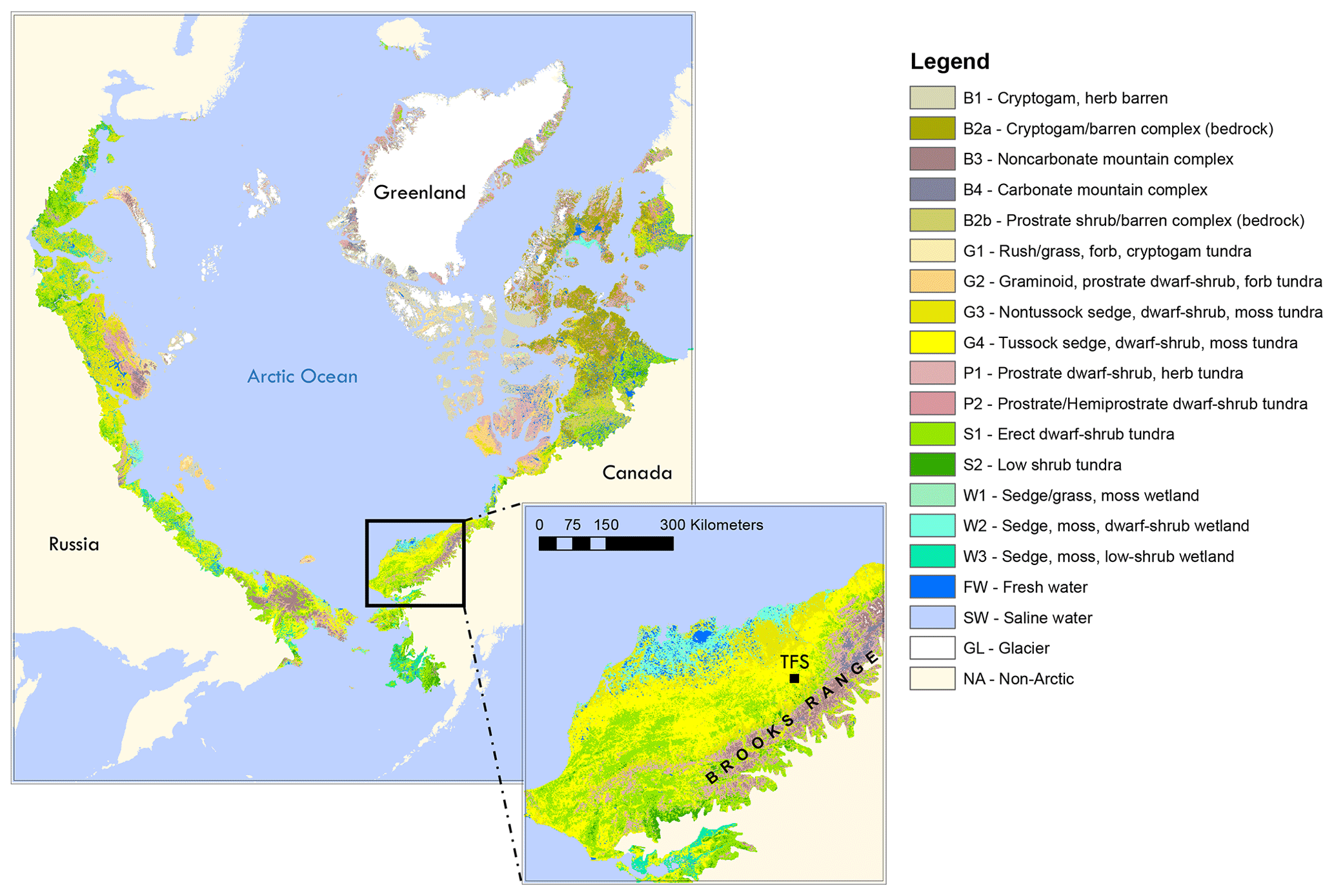
Figure 1Location of Toolik Field Station (TFS) on the north flanks of the Brooks Range in northern Alaska along with arctic vegetation type. This figure was made using the raster version of the circumpolar Arctic vegetation map prepared by Raynolds et al. (2019), which is publicly available at https://www.geobotany.uaf.edu (last access: 19 May 2020).
Emission measurements and atmospheric sampling were conducted from a weatherproof instrument shelter located ∼ 350 m to the west of TFS (see Fig. S1 in the Supplement). Winds at TFS are predominantly from the southerly and northerly sectors (Toolik Field Station Environmental Data Center, 2019), minimizing any influence from camp emissions at the site. Two field campaigns were carried out; the first was from mid-July to mid-August 2018, and the second was from mid-May to the end of June 2019. These two back-to-back campaigns cover the entire growing season (Sullivan et al., 2007), from the onset of snowmelt in mid-May to the first snowfall in mid-August.
2.2 Ambient online measurements of BVOCs and their oxidation products
2.2.1 Gas chromatography and mass spectrometry with flame ionization detector (GC-MS/FID)
An automated gas chromatography and mass spectrometry with flame ionization detector (GC-MS/FID) system was deployed for continuous measurements of atmospheric BVOCs at ∼ 2 h time resolution during the 2018 and 2019 field campaigns. In addition, the system was operated remotely following the 2018 campaign (through 15 September) in order to collect background values at the beginning of autumn. Air was pulled continuously from an inlet on a 4 m meteorological tower located approximately 30 m from the instrument shelter (Van Dam et al., 2013). Air passed through a sodium thiosulfate-coated O3 scrubber for selective O3 removal – to prevent sampling losses and artifacts for reactive BVOCs (Helmig, 1997; Pollmann et al., 2005) – and through a moisture trap to dry the air to a dew point of −45 ∘C. The moisture trap was a u-shaped Silcosteel™ tube (stainless steel treated) cooled using thermoelectric coolers. Analytes were concentrated on a Peltier-cooled (−40 ∘C) multistage microadsorbent trap (50 % Tenax-GR and 50 % Carboxen 1016). Analysis was accomplished by thermal desorption and injection for cryogen-free GC using a DB-1 column (60 m × 320 µm × 5 µm) and helium as a carrier gas. The oven temperature was set to 40 ∘C for 6 min, then increased to 260 ∘C at 20 ∘C min−1, and held isothermally at 260 ∘C for 13 min. The column flow was split between an FID and a MS for simultaneous quantification and identification. Blanks and calibration standards were regularly injected from a manifold. Isoprene (m∕z 67 and 68), methacrolein (MACR) and methyl vinyl ketone (MVK) (m∕z 41, 55, and 70), MT (m∕z 68, 93, 121, and 136), and SQT (m∕z 204, 91, 93, 119, and 69) were identified and quantified using the MS in selected ion-monitoring mode (SIM). The response to isoprene was calibrated using a primary gas standard supplied by the National Physical Laboratory (NPL), certified as containing 4.01±0.09 parts per billion (ppb) of isoprene in a nitrogen matrix. The analytical uncertainty for isoprene was estimated at 16 %, based on the certified uncertainty of the standard and on the repeatability of the standard analysis throughout the campaigns. Instrument responses for MACR, MVK, α-pinene, and acetonitrile were calibrated with multicomponent standards containing 1007 ppb MACR, 971 ppb MVK, 967 ppb α-pinene, and 1016 ppb acetonitrile (Apel-Riemer Environmental Inc., Miami, FL, USA) dynamically diluted into a stream of ultra-zero-grade air to ∼ 3 ppb. Quantification of other terpenoid compounds was based on GC peak area (FID response) plus relative response factors using the effective carbon number concept (Faiola et al., 2012; Scanlon and Willis, 1985). The limit of quantification (LOQ) was ∼ 2 parts per trillion by volume – pptv (pmol mol−1 by volume). In order to monitor and correct for long-term trends in the detection system, including detector drift and decreasing performance of the adsorbent trap, we used peak areas for long-lived chlorofluorocarbons (CFCs) that were monitored in the air samples together with the BVOCs as an internal reference standard. The atmospheric trace gases, CCl3F (CFC-11) and CCl2FCCl2F2 (CFC-113), are ideal in this regard because they are ubiquitous in the atmosphere and exhibit little spatial and temporal variability (Karbiwnyk et al., 2003; Wang et al., 2000).
2.2.2 Proton transfer reaction time-of-flight mass spectrometry (PTR-ToF-MS)
During the summer 2019 campaign, isoprene mixing ratios in ambient air were also measured by proton transfer reaction time-of-flight mass spectrometry (PTR-ToF-MS; model 4000, Ionicon Analytik GmbH, Innsbruck, Austria). The sample inlet was located on the 4 m meteorological tower, right next to the GC-MS/FID inlet. In brief, ambient air was continuously pulled through the PTR-ToF-MS drift tube, where volatile organic compounds (VOCs) with proton affinities higher than that of water (>165.2 kcal mol−1) were ionized via a proton-transfer reaction with primary H3O+ ions, then subsequently separated and detected by a time-of-flight mass spectrometer (with a mass resolving power up to 4000). At TFS, the PTR-ToF-MS measured ions from m∕z 17–400 every 2 min. Ambient air was drawn to the instrument at 10–15 L min−1 via ∼ 30 m of (6.35 mm) outer diameter (OD) perfluoroalkoxy (PFA) tubing maintained at ∼ 55 ∘C and then subsampled by the instrument through ∼ 100 cm of (1.59 mm) OD polyetheretherketone (PEEK) tubing maintained at 60 ∘C. The residence time from the inlet on the 4 m meteorological tower to the drift tube was less than 5 s. Instrument backgrounds were quantified approximately every 5 h for 20 min during the campaign by measuring VOC-free air generated by passing ambient air through a heated catalytic converter (375 ∘C, platinum bead, 1 wt % Pt; Sigma Aldrich). Calibrations were typically performed every 4 d via dynamic dilution of certified gas standard mixtures containing 25 distinct VOCs, including isoprene (Apel-Riemer Environmental Inc., Miami, FL). Here, we report isoprene mixing ratios in order to intercompare them with GC-MS measurements; other species will be reported in future work. The measurement uncertainty for isoprene is ∼ 25 %, which includes uncertainties in the gas standards, calibration method, and data processing.
2.2.3 Instrument intercomparison
Figure S2 shows a comparison of the GC-MS and PTR-ToF-MS isoprene mixing ratios in ambient air. With a correlation coefficient of 0.93 and a linear regression slope of 0.7–1.0, the two measurements agreed within their combined measurement uncertainties, in line with earlier intercomparison studies (e.g., Dunne et al., 2018; de Gouw et al., 2003). Similarly, we found a correlation coefficient of 0.96 between GC-MS and PTR-ToF-MS MVK and MACR mixing ratios (not shown). The good agreement between these two independent techniques gives us confidence that the ambient air results presented here are robust.
2.3 Ambient air vertical profiles
Vertical isoprene mixing ratio profiles were obtained using a 12 ft. (3.66 m) diameter SkyDoc tethered balloon. A total of eight vertical profiles were performed at ∼ 3 h intervals between 12:30 Alaska standard time (AST; hereafter all times are given in AST) on 15 June 2019 and 11:00 on 16 June 2019 in order to capture a full diurnal cycle (solar noon around 14:00). Sampling packages were connected to the tether line such that resulting sampling heights were ∼ 30, ∼ 100, ∼ 170, and ∼ 240 m above ground level (a.g.l.). One identical sampling package was deployed at the surface. Each sampling package contained an adsorbent cartridge for sample collection (see below) that was connected to a downstream battery-powered SKC pocket pump controlled using a mechanical relay, a programmable Arduino, and a real-time clock. Once the balloon reached its apex (∼ 250–300 m a.g.l.), the five pumps were activated simultaneously, and samples were collected for 30 min to ensure that enough material was collected. It should be noted that changes in wind speed and turbulence during the 30 min sampling period often affected the shape of the tethered line and the sampling altitude, adding further uncertainty to the vertical profiles presented here. At the end of the 30 min sampling period, the balloon was brought back down. The adsorbent cartridges were prepared in-house, using glass tubing (89 mm long × 6.4 mm OD; 4.8 mm inner diameter – ID), and loaded with Tenax-GR and Carboxen 1016 adsorbents (270 mg of each), following established practice (Ortega and Helmig, 2008 and references therein). An inlet ozone scrubber was installed on each cartridge to prevent BVOC sampling losses. Field blanks were collected by opening a cartridge (with no pumped airflow) during each balloon flight. Following collection, adsorbent cartridges were sealed with Teflon-coated brass caps and stored in the dark at ∼ 4 ∘C until the chemical analysis. Samples were analyzed at the University of Colorado Boulder, following the method described in Sect. S1 in the Supplement. Our previous intercomparison of this cartridge–GC-MS/FID method with independent and concurrent PTR-MS observations showed that the two measurements agree to within their combined uncertainties at ∼ 25 % (Hu et al., 2015). Meteorological conditions were monitored and recorded during each balloon flight with a radiosonde (Met One Instruments, Inc., Grants Pass, OR, USA) attached to the tethered line just below the balloon.
2.4 BVOC emission rates
2.4.1 Dynamic enclosure measurements
We used dynamic enclosure systems operated at low residence time to quantify vegetative BVOC emissions, following the procedure described by Ortega et al. (2008) and Ortega and Helmig (2008). Two types of enclosures were used, namely branch and surface chambers. For branch enclosures, a Tedlar® bag (Jensen Inert Products, Coral Springs, FL) was sealed around the trunk side of a branch. For surface enclosures, the bag was placed around a circular Teflon base (25 cm width × 16 cm height; see Fig. 2). For both the branch and surface enclosures, the bag was connected to a purge-air line and a sampling line and positioned around the vegetation, minimizing contact with foliage. While purging the enclosure (see Sect. 2.4.3), the vegetation was allowed to acclimate for 24 h before BVOC sampling began. Samples were collected from the enclosure air, concentrated onto solid-adsorbent cartridges (see Sect. 2.3) with an automated sampler, and analyzed in the laboratory at the University of Colorado Boulder following the campaign (see Sect. S1). Temperature and relative humidity were recorded inside and outside the enclosure (see Fig. 2; S-THB-M002 sensors, HOBO, Onset, Bourne, MA) with a data logger (H21-USB, HOBO, Onset, Bourne, MA). Additionally, photosynthetically active radiation (400–700 nm; S-LIA-M003; HOBO, Onset, Bourne, MA) was measured inside the enclosure. Once installed, enclosures were operated for 2–10 d. The tundra vegetation around TFS is heterogeneous, but the most dominant species (except Rubus chamaemorus) were sampled. Table 1 presents the median relative percent cover of plant species in LTER experimental control plots at TFS (Gough, 2019) and indicates whether plant species were present in surface or bag enclosures. The complete list of species sampled and pictures of the enclosures are shown in Figs. S3–S15; the two sampling sectors are highlighted in Fig. S1. Surface enclosures were divided into three vegetation types, namely Salix spp. (high isoprene emitter), Betula spp. (e.g., Betula nana dominance), and miscellaneous (a mix of different species, including lichens and mosses).
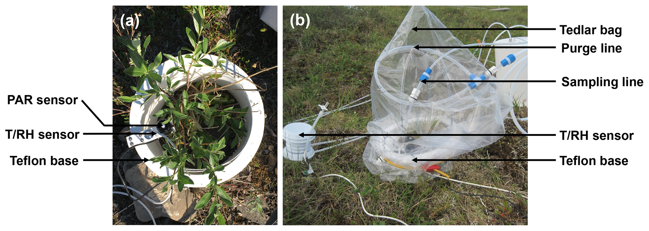
Figure 2Photographs of a surface enclosure experiment setup at Toolik Field Station, Alaska. (a) The first step of the installation consisted of positioning the Teflon base around the vegetation of interest along with temperature (T), relative humidity (RH), and photosynthetically active radiation (PAR) sensors. (b) The second step consisted of positioning the Tedlar® bag around the base. The bag was connected to a purge-air and a sampling line. An additional T∕RH sensor was also positioned outside the bag.
Table 1Year 2017 median relative percent cover of plant species in moist acidic tundra Long-Term Ecological Research (LTER) experimental control plots at Toolik Field Station. The last column indicates whether plant species were present in surface or bag enclosure experiments in this study.

2.4.2 Emission rates
The emission rate (ER in µgC m−2 h−1) for surface enclosures was calculated as follows:
where Cin and Cout are the inlet and outlet analyte concentrations (in µgC L−1), Q is the purge-air flow rate (in L h−1), and S is the surface area of the enclosure (in m2).
The ER for branch enclosures (in µgC g−1 h−1) was calculated as follows:
where mdry is the dried mass (in grams) of leaves enclosed, determined by drying the leaves – harvested after the experiment – at 60–70 ∘C until a consistent weight was achieved (Ortega and Helmig, 2008).
ERs were standardized to 30 ∘C and to a PAR level of 1000 µmol m−2 s−1 using the algorithms described in Guenther et al. (1993, 1995).
2.4.3 Enclosure purge air
Purge air was provided by an upstream, high-capacity oil-free pump providing positive pressure to the enclosure and equipped with an in-line O3 scrubber to avoid a loss in reactive BVOCs from reaction with O3 in the enclosure air and during sampling (Helmig, 1997; Pollmann et al., 2005). The purge-air flow was set to 25 L min−1 and regularly checked using a volumetric flow meter (DryCal Defender, Mesa Labs Bios, Butler, NJ). Excess air escaped from the open end (tied around the Teflon base) while the sample air flow was pulled into the sampling line (see below).
2.4.4 Sample collection
A continuous airflow of 400–500 mL min−1 was drawn from the enclosure through the sampling line. A fraction of this flow was periodically collected at 265–275 mL min−1 on adsorbent cartridges (see Sect. 2.3) using a 10-cartridge autosampler (Helmig et al., 2004). During sampling, cartridges were kept at 40 ∘C, i.e., above ambient temperature, to prevent water accumulation on the adsorbent bed (Karbiwnyk et al., 2002). Samples were periodically collected in series to verify lack of analyte breakthrough. Time-integrated samples were collected for 120 min every 2 h to establish diurnal cycles of BVOC emission. Upon collection, samples were stored in the dark at ∼ 4 ∘C until the chemical analysis at the University of Colorado Boulder.
2.4.5 Internal standards
In order to identify potential BVOC losses during transport, storage, and chemical analysis, 255 of the employed cartridges were preloaded with a four-compound standard mixture prior to the field campaigns. These internal standard compounds (toluene, 1,2,3-trimethylbenzene, 1,2,3,4-tetrahydronaphthalene, and 1,3,5-triisopropylbenzene) were carefully chosen to span a wide range of volatility (C7–C15) and to not interfere (i.e., coelute) with the targeted BVOCs. The recovery of these four compounds was assessed at the end of the campaign, following the analytical procedure described in Sect. S1. Recovery rates were 101.8±13.5 % (toluene), 95.2±20.1 % (1,2,3-trimethylbenzene), 95.6±26.6 % (1,2,3,4-tetrahydronaphthalene), and 100.9±18.7 % (1,3,5-triisopropylbenzene). These results indicate that, overall, BVOC losses during transport, storage, and chemical analysis were negligible. Ortega et al. (2008) previously evaluated the systematic losses of analytes to enclosure systems similar to those used here. The same four-component standard was introduced into the purge-air flow of the enclosures to quantify losses as a function of volatility. That work found median losses of MT and SQT of the order of 20 %–30 %. The emission rates presented here are therefore possibly biased to be lower by a similar amount.
2.5 Peak fitting algorithm
The analysis of ambient air and enclosure chromatograms was performed using the TERN (Thermal desorption aerosol gas chromatography ExploreR and iNtegration package) peak fitting tool implemented in Igor Pro and available online at https://sites.google.com/site/terninigor/ (last access: 19 January 2020; Isaacman-VanWertz et al., 2017).
2.6 Ancillary parameters
Meteorological parameters. A suite of meteorological instruments was deployed on the 4 m tower. Wind speed and direction were measured at ∼ 4 m a.g.l. with a 034B-L sensor (Met One Instruments, Inc., Grants Pass, OR, USA). As described by Van Dam et al. (2013), temperature was measured at three different heights using resistance temperature detector (RTD) temperature probes (model 41342, R. M. Young Company, Traverse City, MI) housed in aspirated radiation shields (model 43502; R. M. Young Company, Traverse City, MI). Regular same-height intercomparisons were conducted to test for instrumental offsets. Incoming and reflected solar radiation were recorded with LI200X pyranometers (Campbell Scientific).
In addition, historical (1988–2019) meteorological data recorded by the TFS Environmental Data Center are available at: https://toolik.alaska.edu/edc/abiotic_monitoring/data_query.php (last access: 15 April 2020).
Particle measurements. A Met One Instruments, Inc., Model 212-2 eight-channel (0.3 to 10 µm) particle profiler was operated continuously on the roof of the weatherproof instrument shelter. This instrument uses a laser-diode-based optical sensor and light-scatter technology to detect, size, and count particles (http://mail.metone.com/particulate-Aero212.htm, last access: 12 February 2020).
Nitrogen oxides. Nitrogen oxides (NOx) were measured with a custom-built, high sensitivity (∼ 5 pptv detection limit) single-channel chemiluminescence analyzer (Fontijn et al., 1970). The instrument monitors nitric oxide (NO) and nitrogen dioxide (NO2) in ambient air using a photolytic converter. Automated switching valves alternated between the NO and NO2 mode every 30 min. Calibration was accomplished by dynamic dilution of a 1.5 parts per million (ppm) compressed NO gas standard (Scott-Marrin, Inc., Riverside, CA).
2.7 Theoretical response of isoprene emissions to temperature in MEGAN2.1
We applied our isoprene emission measurements to evaluate the temperature response algorithms embedded in MEGAN2.1 (Guenther et al., 2012). Theoretical isoprene emission rates (FT) were calculated for TFS as follows:
where CCE is the canopy environment coefficient (assigned a value that results in γT=1 under standard conditions), and εj is the emission factor under standard conditions for vegetation type j with fractional grid box areal coverage κj. We used µg m−2 h−1 at TFS, based on the high resolution (1 km) global emission factor input file available at https://bai.ess.uci.edu/megan/data-and-code/megan21 (last access: 21 May 2020). The temperature activity factor (γT) was calculated as the following:
with
where T is the enclosure ambient air temperature, and T10 is the average enclosure air temperature over the past 10 d.
3.1 Ambient air mixing ratios
3.1.1 Isoprene and oxidation products
Figure 3a and b show the time series of isoprene mixing ratios in ambient air recorded over the course of this study at TFS with the GC system. Mixing ratios were highly variable and ranged from below the quantification limit to 505 pptv (mean of 36.1 pptv). The PTR-ToF-MS gave similar results (see Fig. S16a). These mixing ratios fall within the range of values reported in the Eurasian taiga (e.g., Hakola et al., 2000, 2003; Lappalainen et al., 2009). For example, Hakola et al. (2003) reported a maximum monthly mean mixing ratio of 98 pptv (in July) in central Finland, while Hakola et al. (2000) observed mixing ratios ranging from a few pptv to ∼ 600 pptv in eastern Finland. In general, however, BVOC emissions in the Eurasian taiga are relatively low compared to forest ecosystems in warmer climates and are dominated by monoterpenes (Rinne et al., 2009).
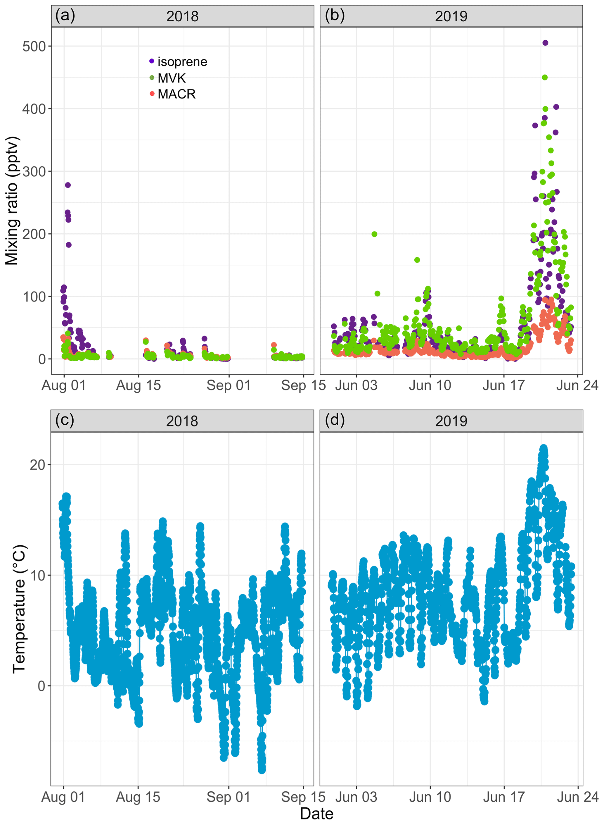
Figure 3Time series of isoprene (purple), methyl vinyl ketone (MVK; green), and methacrolein (MACR; salmon) mixing ratios (in parts per trillion by volume – pptv) in ambient air at Toolik Field station (a, b) and of 30 min averaged ambient temperature (in degrees Celsius) at 4 m above ground level (c, d).
Isoprene mixing ratios peaked on 1 August 2018 around 16:00 and on 20 June 2019 around 22:00, respectively. These two peaks occurred 3–5 h after the daily maximum ambient temperature was reached (17.8 ∘C in 2019 and 21.8 ∘C in 2019; see Fig. 3). The isoprene peak on 20 June 2019 was concomitant with enhanced acetonitrile mixing ratios and particle counts (see Fig. 4), reflecting unusually hazy conditions that day at TFS. We attribute the particle and acetonitrile enhancements to intense wildfires occurring across the Arctic Circle at that time, with most of them being in southern Alaska and Siberia (Earth Observatory, 2019). Acetonitrile increased by a factor of 4 during this event, compared to a factor of 21 increase for isoprene. The higher emission factor for acetonitrile vs. isoprene from biomass burning in boreal forests (Akagi et al., 2011) and the relatively short lifetime of isoprene (Atkinson, 2000) indicate that the observed isoprene enhancement was due to fresh local biogenic emissions rather than transported wildfire emissions.
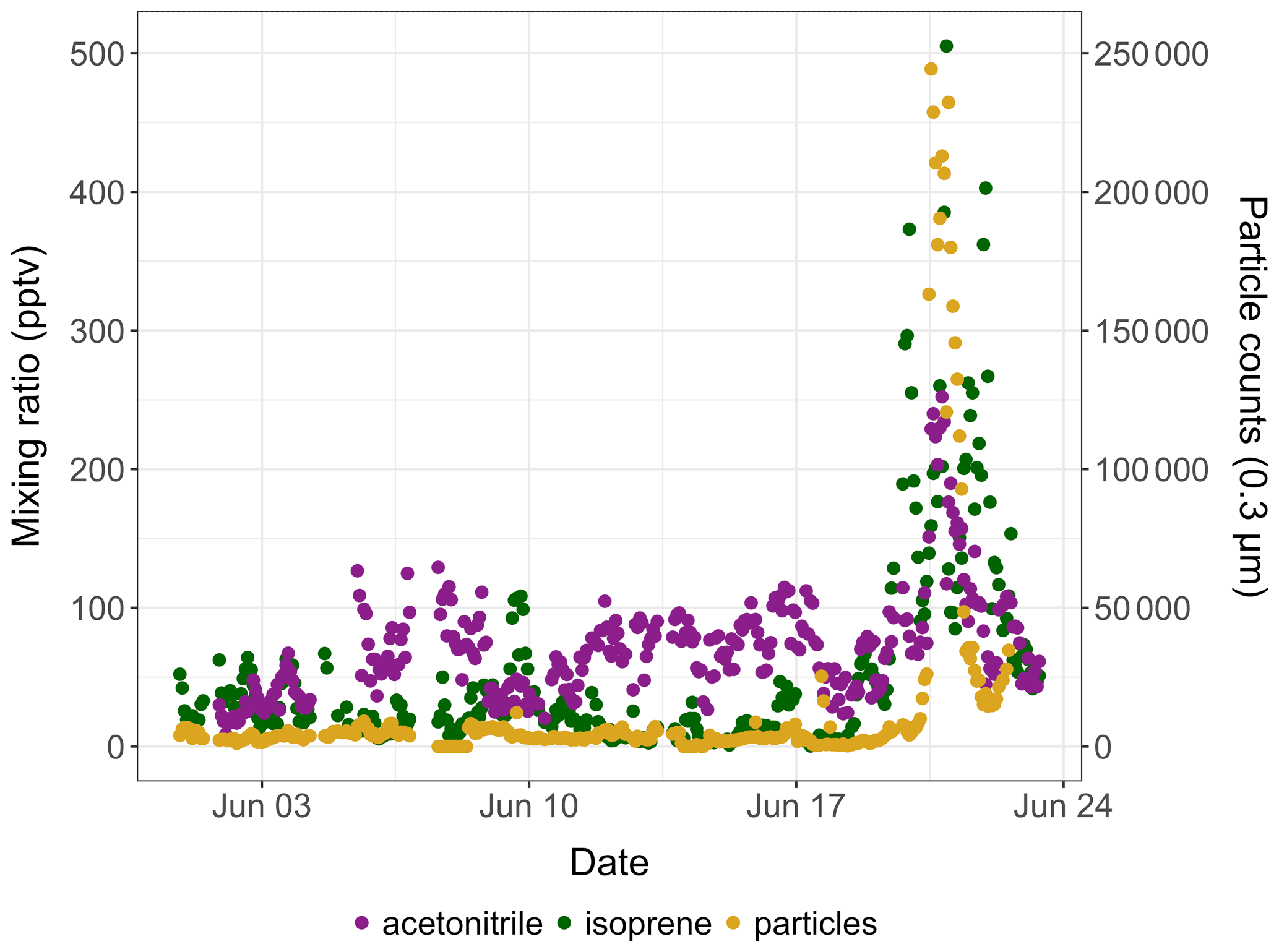
Figure 4Time series of isoprene (green) and acetonitrile (purple) mixing ratios (in pptv) and of 0.3 µm particle counts (yellow) in ambient air at Toolik Field station in June 2019.
Over the course of this study, we recorded MACR and MVK mixing ratios, respectively, ranging from below the quantification limit to 95 pptv (12.4±16.1 pptv; mean ± standard deviation) and from below the quantification limit to 450 pptv (43.1±66.7 pptv; see Fig. 3a, b). The PTR-ToF-MS gave similar results (see Fig. S16b). Median NO and NO2 mixing ratios of 21 and 74 pptv, respectively, during the 2019 campaign (not shown) suggest a low NOx environment, in line with previous studies at several Arctic locations (Bakwin et al., 1992; Honrath and Jaffe, 1992). Under such conditions, MACR and MVK mixing ratios should be used as upper estimates as it has been noted that some low NOx isoprene oxidation products (isoprene hydroxyhydroperoxides) can undergo rearrangement in GC and PTR-MS instruments and be misidentified as MACR and MVK (Rivera-Rios et al., 2014). We found a high correlation between MACR and MVK (R2=0.95, p<0.01) and between these two compounds and isoprene (R2∼0.80, p<0.01). Increases in MACR and MVK mixing ratios above the background were mostly concomitant with isoprene increases, suggesting that atmospheric or within-plant oxidation of isoprene was their main source (Biesenthal et al., 1997; Hakola et al., 2003; Jardine et al., 2012). The mean ratio of MVK to MACR was 2.7, within the range reported by earlier studies (e.g., Apel et al., 2002; Biesenthal and Shepson, 1997; Hakola et al., 2003; Helmig et al., 1998), and no clear diurnal cycle in the ratio was found. This record of ambient air isoprene, MACR, and MVK mixing ratios is, to the best of our knowledge, the first in an Arctic tundra environment. The combined measurement of isoprene and its oxidation products provides a new set of observations to further constrain isoprene chemistry under low NOx conditions in atmospheric models (e.g., Bates and Jacob, 2019).
3.1.2 Isoprene vertical profiles
Figure 5 shows vertical profiles (0 to ∼ 250 m a.g.l.) of isoprene mixing ratios derived from the 30 min tethered balloon samples collected on 15 and 16 June 2019. Temperature profiles (see Fig. S17) indicate that most of the flights were performed in a convective boundary layer (Holton and Hakim, 2013). A nocturnal boundary layer was, however, observed in the first ∼ 50 m from ∼ 02:00 to ∼ 04:30 (see Fig. S17e–f), with temperature increasing with elevation.

Figure 5Vertical profiles of isoprene mixing ratios as inferred from 30 min samples collected with a tethered balloon. The error bars show the analytical uncertainty for isoprene (20 %). Samples with an isoprene mixing ratio lower than blanks were discarded. Times are given as Alaska standard time (UTC−9).
Except during the last flight, isoprene mixing ratios were in the range of background levels (∼ 0–50 pptv) reported with the GC-MS (see Sect. 3.1.1). Samples collected from 10:00–10:30 on 16 June (see Fig. 5h) showed a pronounced gradient, with 200 pptv at ground level and decreasing mixing ratios with elevation. This maximum at ground level is expected for a VOC with a surface source (Helmig et al., 1998), while the 200 pptv mixing ratio can likely be attributed to a temperature-driven increase in isoprene emissions by the surrounding vegetation. Indeed, the ambient temperature at ground level was higher during that flight than during the previous ones (see Fig. S17h). The diurnal cycles of isoprene emissions and temperature are further discussed in Sect. 3.2.2. Interestingly, the GC-MS and the PTR-ToF-MS did not capture this 200 pptv maximum (see Figs. 3 and S16), which may be because the balloon flights were performed at a different location (near sampling sector B; see Fig. S1) surrounded by a higher fraction of isoprene-emitting shrubs (willow).
Samples collected on 16 June 2019 from 04:00 to 04:30 (see Fig. 5f) show decreasing isoprene mixing ratios with increasing elevation, suggesting higher levels (25–50 pptv) in the nocturnal boundary layer than above. This result suggests continuing isoprene emissions by the surrounding vegetation under low PAR conditions. This is further discussed in Sect. 3.2.2.
3.1.3 Monoterpenes and sesquiterpenes
MT mixing ratios ranged from 3 to 537 pptv (14±18 pptv; median ± standard deviation) during the 2019 campaign, according to the PTR-ToF-MS measurements. Using the GC-MS/FID, we were able to detect and quantify the following MT in ambient air: α-pinene, camphene, sabinene, p-cymene, and limonene. Mean mixing ratios are reported in Table 2 (for values lower than the LOQ, mixing ratios equal to half of the LOQ are used). These compounds have been previously identified as emissions of the widespread circumpolar dwarf birch Betula nana (Li et al., 2019; Vedel-Petersen et al., 2015) and other high Arctic vegetation (Schollert et al., 2014). The quantification frequency of camphene, sabinene, p-cymene, and limonene was low (see Table 2), and MT mixing ratios in ambient air were dominated by α-pinene. Several prior studies performed at boreal sites have similarly identified α-pinene as the most abundant monoterpene throughout the growing season (e.g., Hakola et al., 2000; Lindfors et al., 2000; Spirig et al., 2004; Tarvainen et al., 2007). We did not detect any sesquiterpene in ambient air above the 2 pptv instrumental LOQ.
Table 2Average mixing ratios with standard deviation, along with minimum (min) and maximum (max) values and the quantification frequency (QF) of the measured monoterpenes in ambient air. LOQ stands for limit of quantification. For values lower than the LOQ, mixing ratios equal to half of the LOQ were used to calculate the mean.
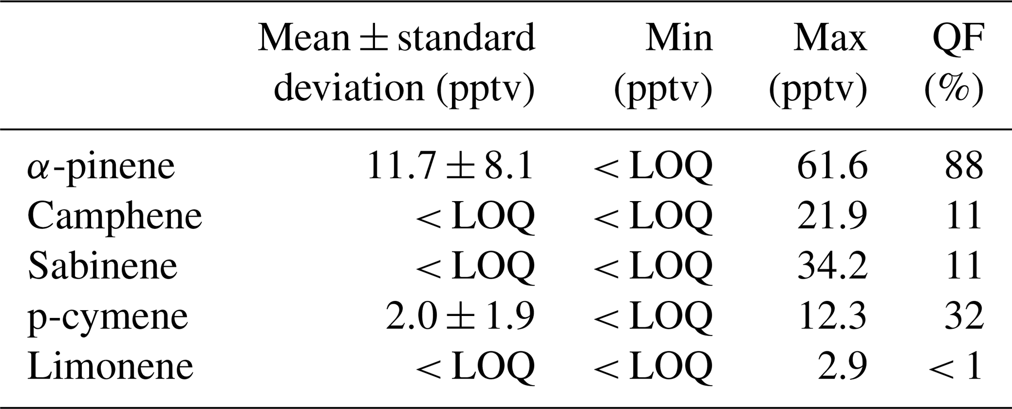
Overall, isoprene and α-pinene dominated the ambient air BVOC profile at TFS, respectively constituting ∼ 72 % and ∼ 24 % of total BVOCs quantified in ambient air (on a mixing-ratio basis).
3.2 Emission rates
3.2.1 Branch enclosures
A branch enclosure experiment was performed from 27 July to 2 August 2018 on Salix glauca to investigate BVOC emission rates per dry weight plant biomass (see Fig. S5). Isoprene emission rates ranged from < 0.01 to 11 µgC g−1 h−1 (with a mean enclosure temperature of 16.5 ∘C and mean PAR of 880 µmol m−2 s−1), in line with nonnormalized emission rates reported at Kobbefjord, Greenland, by Kramshøj et al. (2016; Table 5 in their Supplement) for the same species under slightly different environmental conditions (mean temperature of 24.6 ∘C and mean PAR of 1052 µmol m−2 s−1). Once standardized to 30 ∘C and 1000 µmol m−2 s−1, our emission rates averaged 5 µgC g−1 h−1, in good agreement with standardized emissions reported at Kobbefjord (mean of 7 µgC g−1 h−1) by Vedel-Petersen et al. (2015). The quantified MTs had emissions averaging 2 orders of magnitude lower than those of isoprene (0.01 vs. 1 µgC g−1 h−1). Emission rates for the sum of α-pinene, β-pinene, limonene, camphene, and 1,8-cineole ranged from <0.01 to 0.06 µgC g−1 h−1. These results are again in good agreement with those reported for the same species at Kobbefjord (∼ 0.01 µgC g−1 h−1) by Kramshøj et al. (2016; Table 5 in their Supplement).
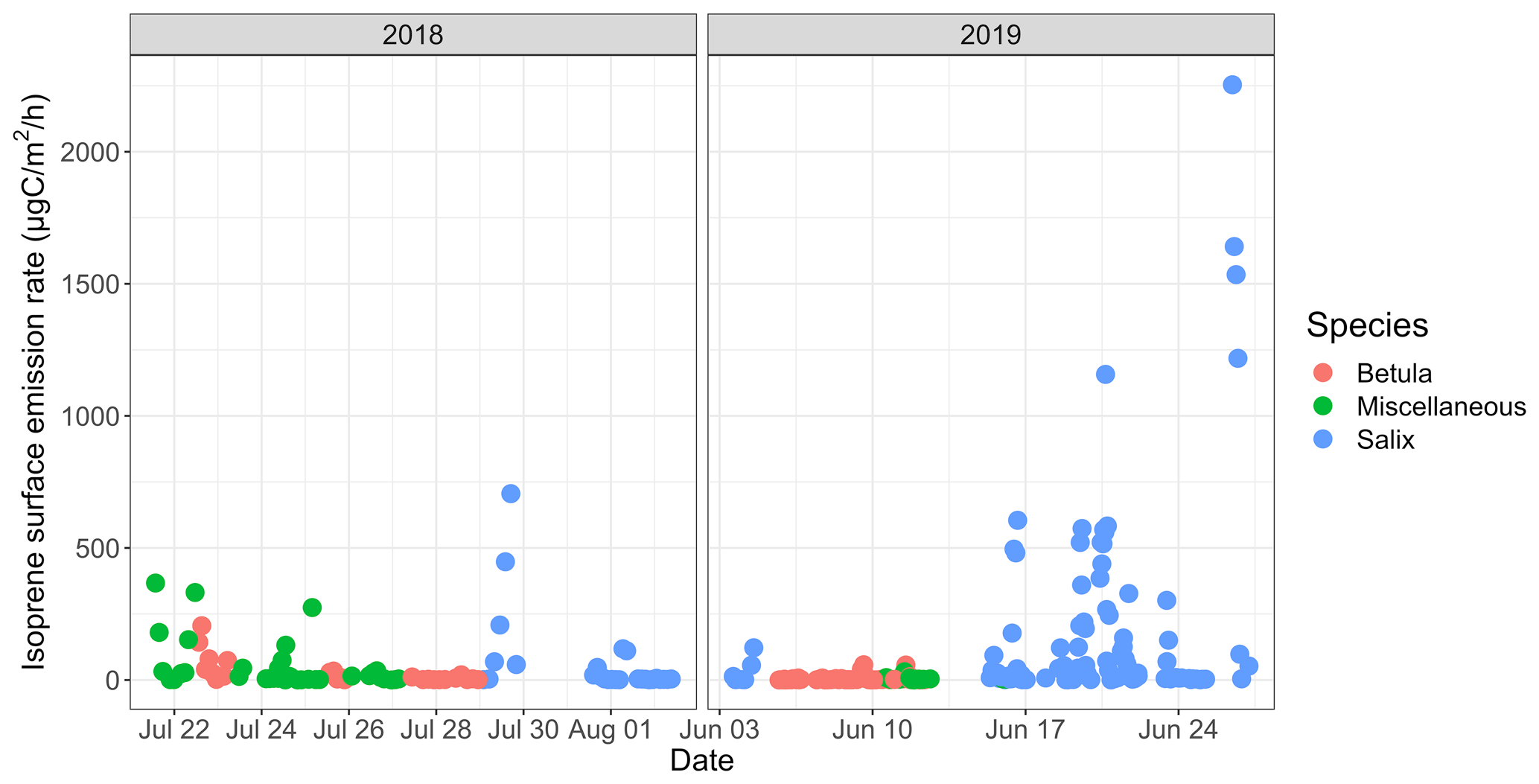
Figure 6Time series of isoprene surface emission rates (in µgC m−2 h−1) for different vegetation types. Miscellaneous refers to a mix of different species, including lichens and moss tundra.
3.2.2 Surface emission rates
The isoprene surface emission rate, as inferred from surface enclosures, was highly variable and ranged from 0.2 to ∼ 2250 µgC m−2 h−1 (see Fig. 6). The 2250 µgC m−2 h−1 maximum, reached on 26 June 2019, with an enclosure temperature of 32 ∘C, is higher than maximum values reported at TFS by Potosnak et al. (2013) (1200 µgC m−2 h−1 at an air temperature of 22 ∘C). It should be noted that these maximum values were observed at different ambient temperatures; we further investigate the temperature dependency of isoprene emissions in Sect. 3.3. Elevated surface emission rates (i.e., >500 µgC m−2 h−1) were all observed while sampling enclosures dominated by Salix spp. At TFS, the overall 24 h mean isoprene emission rate amounted to 85 µgC m−2 h−1, while the daytime (10:00–20:00) and midday (11:00–14:00) means were 140 and 213 µgC m−2 h−1, respectively. To put this in perspective, the average isoprene surface emission rate standardized to 30 ∘C and 1000 µmol m−2 s−1 (∼ 300 µgC m−2 h−1) was an order of magnitude lower than emission rates reported for warmer midlatitude or tropical forests. For example, average midday fluxes of 3000 µgC m−2 h−1 were reported in a northern hardwood forest in Michigan (Pressley et al., 2005), while several reports of isoprene emissions from tropical ecosystems give daily estimates of 2500–3000 µgC m−2 h−1 (Helmig et al., 1998; Karl et al., 2004; Rinne et al., 2002).

Figure 7Surface emission rates of various monoterpenes (in µgC m−2 h−1) for different vegetation types. The lower and upper hinges correspond to the first and third quartiles. The upper (lower) whisker extends from the hinge to the largest (smallest) value no further than 1.5×IQR from the hinge, where IQR is the interquartile range (i.e., the distance between the first and third quartiles). The notches extend and give a ∼ 95 % confidence interval for medians. Miscellaneous refers to a mix of different species, including lichens and moss tundra.
Figure 7 shows the measured surface emission rates for α-pinene, β-pinene, limonene, and 1,8-cineole. While p-cymene, sabinene, 3-carene, and isocaryophyllene (SQT) were detected in some of the surface enclosure samples, we focus the discussion on the most frequently quantified compounds. It is worth noting that the most frequently observed compounds in enclosure samples are among the most frequently seen MT in ambient air (see Sect. 3.1.3). Regardless of the species, emission rates remained, on average, below 1 µgC m−2 h−1 over the course of the study (see Table 3). These results are at the low end of emission rates reported for four vegetation types in high Arctic Greenland (Schollert et al., 2014) but are in line with results reported at Kobbefjord, Greenland, by Kramshøj et al. (2016; Table 4 in their Supplement).
Table 3Isoprene and monoterpenes (sum of α-pinene, β-pinene, limonene, and 1,8-cineole) surface emission rates per vegetation type. Miscellaneous refers to a mix of different species, including lichens and moss tundra (see Figs. S3–S15). Daytime refers to 10:00–20:00, midday to 11:00–14:00, and nighttime to 23:00–05:00 (Alaska standard time – UTC−9). The values in parentheses represent the average enclosure temperature for each emission rate.

Figure 8a–c show the mean diurnal cycle (over the two campaigns) of isoprene surface emission rates for different vegetation types (see Fig. S3–S15 for nomenclature). The two field campaigns were carried out during the midnight sun period, which could possibly sustain BVOC emissions during nighttime. It should, however, be noted that low sun angles translate to very low PAR, and a typical diurnal pattern is observed in summer at TFS despite 24 h of light (see Fig. 8h). Regardless of the vegetation type, isoprene emission rates exhibited a significant diurnal cycle with an early afternoon maximum, in line with the mean diurnal cycle of the enclosure temperature and PAR. These results are in line with the well-established diurnal variation in BVOC emissions in environments ranging from Mediterranean to boreal forests (e.g., Fares et al., 2013; Liu et al., 2004; Ruuskanen et al., 2005; Zini et al., 2001) and with the correlation between isoprene ambient air mixing ratios and temperature at TFS (see Sect. 3.1). Despite the relatively low MT emission rates, a significant diurnal cycle was also observed, with peak total MT emissions of ∼ 1 µgC m−2 h−1 during early afternoon for both Salix spp. and Betula spp. (Fig. 8e–f). A summary of emission rates per vegetation type and time of day is given in Table 3. As can be seen in Table 3 and Fig. 8, PAR and BVOC emissions significantly decreased at night but were still detectable. These sustained BVOC emissions during nighttime confirm observations by Lindwall et al. (2015) during a 24 h experiment with five different Arctic vegetation communities and explain the higher isoprene levels observed in rather than above the nocturnal boundary layer during the diurnal balloon experiment (see Sect. 3.1.2).
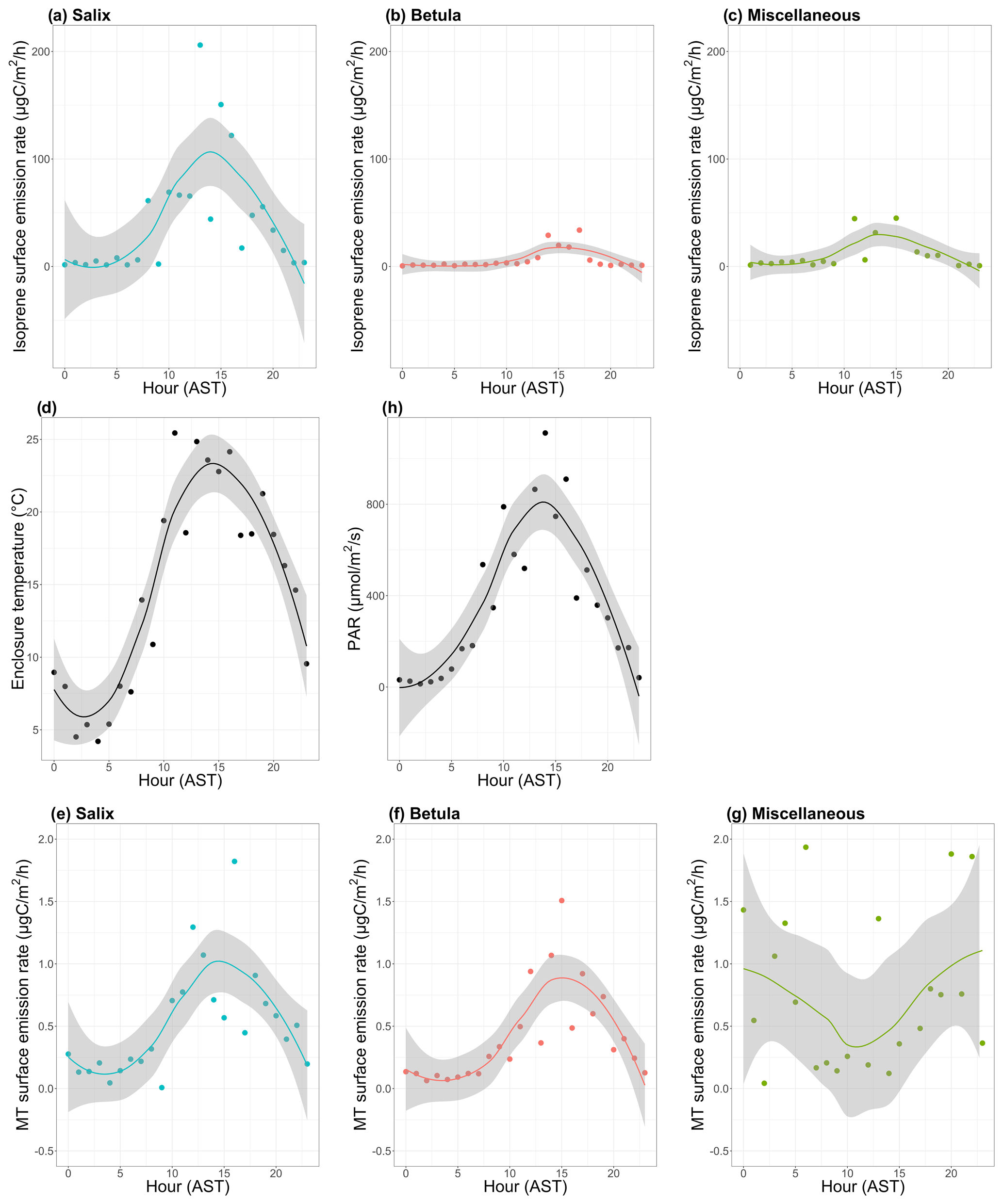
Figure 8Mean diurnal cycle of isoprene (a–c) and monoterpenes (MT; e–g) surface emission rates (in µgC m−2 h−1; note the difference scale on the y axis), (d) enclosure temperature (in degrees Celsius), and (h) enclosure photosynthetically active radiation (PAR in µmol m−2 s−1). The dots represent the hourly means. The line is the smoothed conditional mean while the gray shaded region indicates the 95 % confidence interval. Hours are in Alaska standard time (UTC−9) and correspond to the end of the 2 h sampling period for isoprene and MT emission rates. MT corresponds here to the sum of α-pinene, β-pinene, limonene, and 1,8-cineole. Miscellaneous refers to a mix of different species, including lichens and moss tundra.
The ratio of total MT (given by the sum of α-pinene, β-pinene, limonene, and 1,8-cineole) emissions to isoprene emissions was an order of magnitude higher for Betula spp. (0.22) than for Salix spp. (0.03). This result, driven by the relatively lower isoprene emissions of Betula spp., is in line with earlier studies, suggesting similar emission characteristics for Arctic plants (e.g., Kramshøj et al., 2016; Vedel-Petersen et al., 2015).
4.1 Response of isoprene emissions to temperature
The Arctic has warmed significantly during the last three decades and temperatures are projected to increase by an additional 5–13 ∘C by the end of the century (Overland et al., 2014). Heat wave frequency is also increasing in the terrestrial Arctic (Dobricic et al., 2020). For example, western Siberia experienced an unusually warm May in 2020, with temperatures of 20–25 ∘C (Freedman and Cappucci, 2020). In that context, numerous studies have pointed out the likelihood of increased BVOC emissions due to Arctic warming and associated vegetation and land cover change (Faubert et al., 2010; Potosnak et al., 2013; Rinnan et al., 2011; Tiiva et al., 2008).
Over the course of the two field campaigns at TFS, BVOC surface emission rates were measured over a large span of enclosure temperatures (2–41 ∘C). While isoprene and MT emissions respond to leaf temperature (Guenther et al., 1993), air temperature was used here instead of leaf temperature, which has been assumed before in the literature for high-latitude ecosystems (e.g., Olofsson et al., 2005; Potosnak et al., 2013). Several studies have, however, suggested a decoupling of leaf and air temperature in tundra environments (Lindwall et al., 2016; Potosnak et al., 2013). With a predicted increase in air temperature in the Arctic, it still remains largely unknown how leaf temperature will change and impact BVOC emissions. As suggested by Tang et al. (2016), long-term parallel observations of both leaf and air temperature are needed. The response of BVOC emissions to temperature discussed here should be interpreted with this potential caveat in mind.
While MT emissions remained low and close to the detection limit, thus preventing robust quantification of any emission–temperature relationship, isoprene emissions significantly increased with temperature (Fig. 9). Figure 9 combines daytime (e.g., with relatively high PAR values) isoprene emission rates from different surface enclosures, with results normalized to account for differing total biomass and species distributions (with Salix spp. being the dominant emitter). Specifically, we divided all fluxes by the enclosure-specific mean emission at 20±1 ∘C. Emission rates are often standardized to 30 ∘C, but we employ 20 ∘C here owing to the colder growth environment at TFS (Ekberg et al., 2009). The isoprene emission–temperature relationship observed at TFS (in blue) is very similar to that reported by Tang et al. (2016) at Abisko (Sweden; in pink) for tundra heath (dominated by evergreen and deciduous dwarf shrubs). Results at TFS and Abisko both point to a high isoprene temperature response for Arctic ecosystems (Tang et al., 2016). This is further supported by two warming experiments performed in mesic tundra heath (dominated by Betula nana, Empetrum nigrum, Empetrum hermaphroditum, and Cassiope tetragona) and dry dwarf shrub tundra (codominated by Empetrum hermaphroditum and Salix glauca) in western Greenland (Kramshøj et al., 2016; Lindwall et al., 2016). Kramshøj et al. (2016) observed a 240 % isoprene emission increase with 3 ∘C warming, while Lindwall et al. (2016) reported a 280 % increase with 4 ∘C warming. The observationally derived emission–temperature relationship derived here for TFS reveals a 180 %–215 % emission increase with 3–4 ∘C warming.

Figure 9Normalized isoprene surface emission rate (emissions at 20 ∘C set equal to 1.0) as a function of enclosure temperature (in degrees Celsius). This figure shows the response to temperature as observed at Toolik Field Station (TFS, in blue) and Abisko, Sweden (in pink; Tang et al., 2016), and as parameterized in MEGAN2.1 (in green). The blue solid line is the exponential fit at TFS. The term n denotes the number of measurements in each enclosure temperature bin. It should be noted that the enclosure temperature was on average 5–6 ∘C warmer than ambient air due to greenhouse heating.
The MEGAN2.1 modeling framework is commonly used to estimate BVOC fluxes between terrestrial ecosystems and the atmosphere (e.g., Millet et al., 2018). Here, we apply the TFS observations to evaluate the MEGAN2.1 emission–temperature relationship for this Arctic environment. Figure 9 shows that the model temperature algorithm provides a close fit with observations below 30 ∘C, with a 170 %–240 % emission increase for a 3–4 ∘C warming. While the model predicts a leveling-off of emissions at approximately 30–35 ∘C, our observations reveal no such phenomenon within the 0–40 ∘C enclosure temperature range (Fig. 9). However, given the limited number of enclosure measurements above 30 ∘C, a leveling off of emissions cannot be statistically ruled out. The key result here is that MEGAN2.1 adequately reproduces the temperature dependence response of Arctic ecosystems in the 0–30 ∘C temperature range, with ambient temperature >30 ∘C being unlikely. The highest air temperature on record at TFS (1988–2019) is 26.5 ∘C, and the mean summertime (June–August) temperature over that period is 9 ∘C. Additionally, for each year in the 1988–2019 historical data set, there were only 1 to 23 d (0 to 4 d) per year with a maximum temperature above 20 ∘C (above 25 ∘C). If global greenhouse gas emissions continue to increase, temperatures are expected to rise 6–7 ∘C in northern Alaska by the end of the century (annual average; Markon et al., 2012), while the number of days with temperatures above 25 ∘C could triple (Lader et al., 2017). Based on current climate conditions and this rate of change, the MEGAN2.1 algorithm adequately represents the temperature dependence response of Arctic ecosystems for the near and intermediate-term future.
4.2 Long-term effects of warming
BVOCs produced by plants are involved in plant growth, reproduction, and defense, and plants use isoprene emissions as a thermotolerance mechanism (Peñuelas and Staudt, 2010; Sasaki et al., 2007). The exponential response of isoprene emissions to temperature observed at TFS adds to a growing body of evidence indicating a high isoprene temperature response in Arctic ecosystems. However, observations at TFS do not necessarily reflect long-term effects of warming. Schollert et al. (2015) examined how long-term warming affects the leaf anatomy of individual arctic plant shoots (Betula nana, Cassiope tetragona, Empetrum hermaphroditum, and Salix arctica). They found that long-term warming results in significantly thicker leaves, suggesting anatomical acclimation. While the authors hypothesized that this anatomical acclimation may limit the increase of BVOC emissions at plant shoot level, Kramshøj et al. (2016) later showed that BVOC emissions from Arctic tundra, exposed to 6 years of experimental warming, increase at both the plant shoot and ecosystem levels.
In addition to the direct impact of long-term warming on BVOC emissions, ecosystem level emissions are expected to increase in the Arctic due to climate-driven changes in plant biomass and vegetation composition. For instance, the widespread increase in shrub abundance in the Arctic – due to a longer growing season and enhanced nutrient availability (Berner et al., 2018; Sturm et al., 2001) – will likely significantly affect the BVOC emission potential of the Arctic tundra. Additionally, as mentioned above and as discussed extensively by Peñuelas and Staudt (2010) and Loreto and Schnitlzer (2010), emissions of BVOCs might be largely beneficial for plants, conferring them higher protection from abiotic stressors which are predicted to be more severe in the future. Long-term arctic warming may thus favor BVOC-emitting species even further.
While BVOC ambient concentrations and emission rates have been frequently measured in boreal ecosystems, Arctic tundra environments are under studied. We provide summertime BVOC ambient air mixing ratios and emission rates at Toolik Field Station, on the north flank of the Brooks Range in northern Alaska, here. We present the first continuous summertime record of ambient air isoprene and its first-generation oxidation products in the Arctic tundra environment. This data set provides a new set of observations to constrain isoprene chemistry in low NOx environments. This data set also provides a baseline for investigating future changes in the BVOC emission potential of the Arctic tundra environment. While the overall mean isoprene emission rate amounted to 85 µgC m−2 h−1, elevated (>500 µgC m−2 h−1) isoprene surface emission rates were observed for Salix spp., a known isoprene emitter. We also show that the response to the temperature of isoprene emissions in enclosures dominated by Salix spp. increased exponentially in the 0–40 ∘C range, likely conferring greater thermal protection for these plants. Given the widespread increase in shrub abundance in the Arctic (including Salix spp.), our results support earlier studies (e.g., Valolahti et al., 2015) suggesting that climate-induced changes in the Arctic vegetation composition will significantly affect the BVOC emission potential of the Arctic tundra, with implications for atmospheric oxidation processes and climate feedbacks.
Data are available upon request to the corresponding author.
The supplement related to this article is available online at: https://doi.org/10.5194/bg-17-6219-2020-supplement.
DH, LH, and DBM designed the experiments and acquired funding. HA led the two field campaigns, with significant on-site contributions from KM, JH, LH, DBM, KC, JM, CW, TM, and DH. JH designed and built most of the instruments used in this study. CW acquired the PTR-ToF-MS data during the second campaign, and DK performed data analysis. MSBH identified the plant species and provided guidance during the field campaigns. KM and HA analyzed the samples in the laboratory. HA analyzed all the data and prepared the paper with contributions from all coauthors.
The authors declare that they have no conflict of interest.
The authors would like to thank CH2MHill Polar Services for the logistical support, the Toolik Field Station staff for assistance with the measurements, and Ilann Bourgeois and Georgios Gkatzelis for the helpful discussions. The authors also appreciate the help of Anssi Liikanen, who offered kind assistance when collecting BVOC samples with the tethered balloon, and Wade Permar, who helped with the PTR-ToF-MS measurements. Finally, the authors gratefully acknowledge Claudia Czimczik and Shawn Pedron at the University of California Irvine for letting us use their soil chamber collars.
This research was funded by the National Science Foundation (grant no. 1707569). Undergraduate students Katelyn McErlean, Jacob Moss, and Kaixin Cui received financial support from the University of Colorado Boulder's Undergraduate Research Opportunities Program (UROP; grant nos. 5352323, 4422751, and 4332562, respectively).
This paper was edited by Paul Stoy and reviewed by three anonymous referees.
Akagi, S. K., Yokelson, R. J., Wiedinmyer, C., Alvarado, M. J., Reid, J. S., Karl, T., Crounse, J. D., and Wennberg, P. O.: Emission factors for open and domestic biomass burning for use in atmospheric models, Atmos. Chem. Phys., 11, 4039–4072, https://doi.org/10.5194/acp-11-4039-2011, 2011.
Apel, E. C., Riemer, D. D., Hills, A., Baugh, W., Orlando, J., Faloona, I., Tan, D., Brune, W., Lamb, B., Westberg, H., Carroll, M. A., Thornberry, T., and Geron, C. D.: Measurement and interpretation of isoprene fluxes and isoprene, methacrolein, and methyl vinyl ketone mixing ratios at the PROPHET site during the 1998 Intensive, J. Geophys. Res.-Atmos., 107, ACH 7-1–ACH 7-15, https://doi.org/10.1029/2000JD000225, 2002.
Arneth, A., Harrison, S. P., Zaehle, S., Tsigaridis, K., Menon, S., Bartlein, P. J., Feichter, J., Korhola, A., Kulmala, M., O'Donnell, D., Schurgers, G., Sorvari, S., and Vesala, T.: Terrestrial biogeochemical feedbacks in the climate system, Nat. Geosci., 3, 525–532, https://doi.org/10.1038/ngeo905, 2010.
Atkinson, R.: Atmospheric chemistry of VOCs and NOx, Atmos. Environ., 34, 2063–2101, https://doi.org/10.1016/S1352-2310(99)00460-4, 2000.
Bakwin, P. S., Wofsy, S. C., Fan, S.-M., and Fitzjarrald, D. R.: Measurements of NOx and NOy concentrations and fluxes over Arctic tundra, J. Geophys. Res.-Atmos., 97, 16545–16557, https://doi.org/10.1029/91JD00929, 1992.
Bates, K. H. and Jacob, D. J.: A new model mechanism for atmospheric oxidation of isoprene: global effects on oxidants, nitrogen oxides, organic products, and secondary organic aerosol, Atmos. Chem. Phys., 19, 9613–9640, https://doi.org/10.5194/acp-19-9613-2019, 2019.
Berner, L. T., Jantz, P., Tape, K. D., and Goetz, S. J.: Tundra plant above-ground biomass and shrub dominance mapped across the North Slope of Alaska, Environ. Res. Lett., 13, 035002, https://doi.org/10.1088/1748-9326/aaaa9a, 2018.
Biesenthal, T. A. and Shepson, P. B.: Observations of anthropogenic inputs of the isoprene oxidation products methyl vinyl ketone and methacrolein to the atmosphere, Geophys. Res. Lett., 24, 1375–1378, https://doi.org/10.1029/97GL01337, 1997.
Biesenthal, T. A., Wu, Q., Shepson, P. B., Wiebe, H. A., Anlauf, K. G., and Mackay, G. I.: A study of relationships between isoprene, its oxidation products, and ozone, in the Lower Fraser Valley, BC – ScienceDirect, Atmos. Environ., 31, 2049–2058, 1997.
Carlton, A. G., Wiedinmyer, C., and Kroll, J. H.: A review of Secondary Organic Aerosol (SOA) formation from isoprene, Atmos. Chem. Phys., 9, 4987–5005, https://doi.org/10.5194/acp-9-4987-2009, 2009.
de Gouw, J. A., Goldan, P. D., Warneke, C., Kuster, W. C., Roberts, J. M., Marchewka, M., Bertman, S. B., Pszenny, A. A. P., and Keene, W. C.: Validation of proton transfer reaction-mass spectrometry (PTR-MS) measurements of gas-phase organic compounds in the atmosphere during the New England Air Quality Study (NEAQS) in 2002, J. Geophys. Res.-Atmos., 108, 4682, https://doi.org/10.1029/2003JD003863, 2003.
Dobricic, S., Russo, S., Pozzoli, L., Wilson, J., and Vignati, E.: Increasing occurrence of heat waves in the terrestrial Arctic, Environ. Res. Lett., 15, 024022, https://doi.org/10.1088/1748-9326/ab6398, 2020.
Dunne, E., Galbally, I. E., Cheng, M., Selleck, P., Molloy, S. B., and Lawson, S. J.: Comparison of VOC measurements made by PTR-MS, adsorbent tubes–GC-FID-MS and DNPH derivatization–HPLC during the Sydney Particle Study, 2012: a contribution to the assessment of uncertainty in routine atmospheric VOC measurements, Atmos. Meas. Tech., 11, 141–159, https://doi.org/10.5194/amt-11-141-2018, 2018.
Earth Observatory: Arctic Fires Fill the Skies with Soot, available at: https://earthobservatory.nasa.gov/images/145380/arctic-fires-fill-the-skies-with-soot#targetText=In June and July 2019,harmful particles into the air, last access: 16 October 2019.
Ekberg, A., Arneth, A., Hakola, H., Hayward, S., and Holst, T.: Isoprene emission from wetland sedges, Biogeosciences, 6, 601–613, https://doi.org/10.5194/bg-6-601-2009, 2009.
Ekberg, A., Arneth, A., and Holst, T.: Isoprene emission from Sphagnum species occupying different growth positions above the water table, Boreal Environ. Res. Int. Interdiscip. J., 16, 47–59, 2011.
Elmendorf, S. C., Henry, G. H. R., Hollister, R. D., Björk, R. G., Boulanger-Lapointe, N., Cooper, E. J., Cornelissen, J. H. C., Day, T. A., Dorrepaal, E., Elumeeva, T. G., Gill, M., Gould, W. A., Harte, J., Hik, D. S., Hofgaard, A., Johnson, D. R., Johnstone, J. F., Jónsdóttir, I. S., Jorgenson, J. C., Klanderud, K., Klein, J. A., Koh, S., Kudo, G., Lara, M., Lévesque, E., Magnússon, B., May, J. L., Mercado-Díaz, J. A., Michelsen, A., Molau, U., Myers-Smith, I. H., Oberbauer, S. F., Onipchenko, V. G., Rixen, C., Schmidt, N. M., Shaver, G. R., Spasojevic, M. J., Þórhallsdóttir, Þ. E., Tolvanen, A., Troxler, T., Tweedie, C. E., Villareal, S., Wahren, C.-H., Walker, X., Webber, P. J., Welker, J. M., and Wipf, S.: Plot-scale evidence of tundra vegetation change and links to recent summer warming, Nat. Clim. Change, 2, 453–457, https://doi.org/10.1038/nclimate1465, 2012.
Faiola, C. L., Erickson, M. H., Fricaud, V. L., Jobson, B. T., and VanReken, T. M.: Quantification of biogenic volatile organic compounds with a flame ionization detector using the effective carbon number concept, Atmos. Meas. Tech., 5, 1911–1923, https://doi.org/10.5194/amt-5-1911-2012, 2012.
Fares, S., Schnitzhofer, R., Jiang, X., Guenther, A., Hansel, A., and Loreto, F.: Observations of Diurnal to Weekly Variations of Monoterpene-Dominated Fluxes of Volatile Organic Compounds from Mediterranean Forests: Implications for Regional Modeling, Environ. Sci. Technol., 47, 11073–11082, https://doi.org/10.1021/es4022156, 2013.
Faubert, P., Tiiva, P., Rinnan, Å., Michelsen, A., Holopainen, J. K., and Rinnan, R.: Doubled volatile organic compound emissions from subarctic tundra under simulated climate warming, New Phytol., 187, 199–208, https://doi.org/10.1111/j.1469-8137.2010.03270.x, 2010.
Fehsenfeld, F., Calvert, J., Fall, R., Goldan, P., Guenther, A. B., Hewitt, C. N., Lamb, B., Liu, S., Trainer, M., Westberg, H., and Zimmerman, P.: Emissions of volatile organic compounds from vegetation and the implications for atmospheric chemistry, Glob. Biogeochem. Cy., 6, 389–430, https://doi.org/10.1029/92GB02125, 1992.
Fontijn, A., Sabadell, A. J., and Ronco, R. J.: Homogeneous chemiluminescent measurement of nitric oxide with ozone. Implications for continuous selective monitoring of gaseous air pollutants, Anal. Chem., 42, 575–579, https://doi.org/10.1021/ac60288a034, 1970.
Forbes, B. C., Fauria, M. M., and Zetterberg, P.: Russian Arctic warming and “greening” are closely tracked by tundra shrub willows, Glob. Change Biol., 16, 1542–1554, https://doi.org/10.1111/j.1365-2486.2009.02047.x, 2010.
Freedman, A. and Cappucci, M.: Parts of Siberia are hotter than Washington, with temperatures nearly 40 degrees above average, Wash. Post, 22 May, available at: https://www.washingtonpost.com/weather/2020/05/22/siberia-heat-wave/, last access: 29 May 2020.
Fuentes, J. D., Lerdau, M., Atkinson, R., Baldocchi, D., Bottenheim, J. W., Ciccioli, P., Lamb, B., Geron, C., Gu, L., Guenther, A., Sharkey, T. D., and Stockwell, W.: Biogenic Hydrocarbons in the Atmospheric Boundary Layer: A Review, B. Am. Meteorol. Soc., 81, 1537–1576, https://doi.org/10.1175/1520-0477(2000)081<1537:BHITAB>2.3.CO;2, 2000.
Gough, L.: Relative percent cover of plant species for years 2012–2017 in the Arctic Long-term Ecological Research (ARC-LTER) 1989 moist acidic tundra (MAT89) experimental plots, Toolik Field Station, Alaska, EDI Data Portal, https://doi.org/10.6073/PASTA/F31DEF760DB3F8E6CFEE5FEE07CC693E, 2019.
Guenther, A., Hewitt, C. N., Erickson, D., Fall, R., Geron, C., Graedel, T., Harley, P., Klinger, L., Lerdau, M., Mckay, W. A., Pierce, T., Scholes, B., Steinbrecher, R., Tallamraju, R., Taylor, J., and Zimmerman, P.: A global model of natural volatile organic compound emissions, J. Geophys. Res.-Atmos., 100, 8873–8892, https://doi.org/10.1029/94JD02950, 1995.
Guenther, A., Karl, T., Harley, P., Wiedinmyer, C., Palmer, P. I., and Geron, C.: Estimates of global terrestrial isoprene emissions using MEGAN (Model of Emissions of Gases and Aerosols from Nature), Atmos. Chem. Phys., 6, 3181–3210, https://doi.org/10.5194/acp-6-3181-2006, 2006.
Guenther, A. B., Zimmerman, P. R., Harley, P. C., Monson, R. K., and Fall, R.: Isoprene and monoterpene emission rate variability: Model evaluations and sensitivity analyses, J. Geophys. Res.-Atmos., 98, 12609–12617, https://doi.org/10.1029/93JD00527, 1993.
Guenther, A. B., Jiang, X., Heald, C. L., Sakulyanontvittaya, T., Duhl, T., Emmons, L. K., and Wang, X.: The Model of Emissions of Gases and Aerosols from Nature version 2.1 (MEGAN2.1): an extended and updated framework for modeling biogenic emissions, Geosci. Model Dev., 5, 1471–1492, https://doi.org/10.5194/gmd-5-1471-2012, 2012.
Hakola, H., Laurila, T., Rinne, J., and Puhto, K.: The ambient concentrations of biogenic hydrocarbons at a northern European, boreal site, Atmos. Environ., 34, 4971–4982, https://doi.org/10.1016/S1352-2310(00)00192-8, 2000.
Hakola, H., Tarvainen, V., Laurila, T., Hiltunen, V., Hellén, H., and Keronen, P.: Seasonal variation of VOC concentrations above a boreal coniferous forest, Atmos. Environ., 37, 1623–1634, https://doi.org/10.1016/S1352-2310(03)00014-1, 2003.
Helmig, D.: Ozone removal techniques in the sampling of atmospheric volatile organic trace gases, Atmos. Environ., 31, 3635–3651, https://doi.org/10.1016/S1352-2310(97)00144-1, 1997.
Helmig, D., Balsley, B., Davis, K., Kuck, L. R., Jensen, M., Bognar, J., Smith, T., Arrieta, R. V., Rodríguez, R., and Birks, J. W.: Vertical profiling and determination of landscape fluxes of biogenic nonmethane hydrocarbons within the planetary boundary layer in the Peruvian Amazon, J. Geophys. Res.-Atmos., 103, 25519–25532, https://doi.org/10.1029/98JD01023, 1998.
Helmig, D., Bocquet, F., Pollmann, J., and Revermann, T.: Analytical techniques for sesquiterpene emission rate studies in vegetation enclosure experiments, Atmos. Environ., 38, 557–572, https://doi.org/10.1016/j.atmosenv.2003.10.012, 2004.
Hollesen, J., Buchwal, A., Rachlewicz, G., Hansen, B. U., Hansen, M. O., Stecher, O., and Elberling, B.: Winter warming as an important co-driver for Betula nana growth in western Greenland during the past century, Glob. Change Biol., 21, 2410–2423, 2015.
Holst, T., Arneth, A., Hayward, S., Ekberg, A., Mastepanov, M., Jackowicz-Korczynski, M., Friborg, T., Crill, P. M., and Bäckstrand, K.: BVOC ecosystem flux measurements at a high latitude wetland site, Atmos. Chem. Phys., 10, 1617–1634, https://doi.org/10.5194/acp-10-1617-2010, 2010.
Holton, J. R. and Hakim, G. J. (Eds.): Chapter 8 – The Planetary Boundary Layer, in: An Introduction to Dynamic Meteorology, 5th Edn., 255–277, Academic Press, Boston, 2013.
Honrath, R. E. and Jaffe, D. A.: The seasonal cycle of nitrogen oxides in the Arctic troposphere at Barrow, Alaska, J. Geophys. Res.-Atmos., 97, 20615–20630, https://doi.org/10.1029/92JD02081, 1992.
Hu, L., Millet, D. B., Baasandorj, M., Griffis, T. J., Turner, P., Helmig, D., Curtis, A. J., and Hueber, J.: Isoprene emissions and impacts over an ecological transition region in the U.S. Upper Midwest inferred from tall tower measurements, J. Geophys. Res.-Atmos., 120, 3553–3571, https://doi.org/10.1002/2014JD022732, 2015.
Isaacman-VanWertz, G., Sueper, D. T., Aikin, K. C., Lerner, B. M., Gilman, J. B., de Gouw, J. A., Worsnop, D. R., and Goldstein, A. H.: Automated single-ion peak fitting as an efficient approach for analyzing complex chromatographic data, J. Chromatogr. A, 1529, 81–92, https://doi.org/10.1016/j.chroma.2017.11.005, 2017.
Jardine, K. J., Monson, R. K., Abrell, L., Saleska, S. R., Arneth, A., Jardine, A., Ishida, F. Y., Serrano, A. M. Y., Artaxo, P., Karl, T., Fares, S., Goldstein, A., Loreto, F., and Huxman, T.: Within-plant isoprene oxidation confirmed by direct emissions of oxidation products methyl vinyl ketone and methacrolein, Glob. Change Biol., 18, 973–984, https://doi.org/10.1111/j.1365-2486.2011.02610.x, 2012.
Kade, A., Bret-Harte, M. S., Euskirchen, E. S., Edgar, C., and Fulweber, R. A.: Upscaling of CO2 fluxes from heterogeneous tundra plant communities in Arctic Alaska, J. Geophys. Res.-Biogeo., 117, G04007, https://doi.org/10.1029/2012JG002065, 2012.
Karbiwnyk, C. M., Mills, C. S., Helmig, D., and Birks, J. W.: Minimization of water vapor interference in the analysis of non-methane volatile organic compounds by solid adsorbent sampling, J. Chromatogr. A, 958, 219–229, https://doi.org/10.1016/s0021-9673(02)00307-2, 2002.
Karbiwnyk, C. M., Mills, C. S., Helmig, D., and Birks, J. W.: Use of chloroflurocarbons as internal standards for the measurement of atmospheric non-methane volatile organic compounds sampled onto solid adsorbent cartridges, Environ. Sci. Technol., 37, 1002–1007, https://doi.org/10.1021/es025910q, 2003.
Karl, T., Potosnak, M., Guenther, A., Clark, D., Walker, J., Herrick, J. D., and Geron, C.: Exchange processes of volatile organic compounds above a tropical rain forest: Implications for modeling tropospheric chemistry above dense vegetation, J. Geophys. Res.-Atmos., 109, D18306, https://doi.org/10.1029/2004JD004738, 2004.
Kramshøj, M., Vedel-Petersen, I., Schollert, M., Rinnan, Å., Nymand, J., Ro-Poulsen, H., and Rinnan, R.: Large increases in Arctic biogenic volatile emissions are a direct effect of warming, Nat. Geosci., 9, 349–352, https://doi.org/10.1038/ngeo2692, 2016.
Kulmala, M., Suni, T., Lehtinen, K. E. J., Dal Maso, M., Boy, M., Reissell, A., Rannik, Ü., Aalto, P., Keronen, P., Hakola, H., Bäck, J., Hoffmann, T., Vesala, T., and Hari, P.: A new feedback mechanism linking forests, aerosols, and climate, Atmos. Chem. Phys., 4, 557–562, https://doi.org/10.5194/acp-4-557-2004, 2004.
Lader, R., Walsh, J. E., Bhatt, U. S., and Bieniek, P. A.: Projections of Twenty-First-Century Climate Extremes for Alaska via Dynamical Downscaling and Quantile Mapping, J. Appl. Meteorol. Clim., 56, 2393–2409, https://doi.org/10.1175/JAMC-D-16-0415.1, 2017.
Lappalainen, H. K., Sevanto, S., Bäck, J., Ruuskanen, T. M., Kolari, P., Taipale, R., Rinne, J., Kulmala, M., and Hari, P.: Day-time concentrations of biogenic volatile organic compounds in a boreal forest canopy and their relation to environmental and biological factors, Atmos. Chem. Phys., 9, 5447–5459, https://doi.org/10.5194/acp-9-5447-2009, 2009.
Li, T., Holst, T., Michelsen, A., and Rinnan, R.: Amplification of plant volatile defence against insect herbivory in a warming Arctic tundra, Nat. Plants, 5, 568–574, https://doi.org/10.1038/s41477-019-0439-3, 2019.
Lim, H.-J., Carlton, A. G., and Turpin, B. J.: Isoprene Forms Secondary Organic Aerosol through Cloud Processing:? Model Simulations, Environ. Sci. Technol., 39, 4441–4446, https://doi.org/10.1021/es048039h, 2005.
Lindfors, V., Laurila, T., Hakola, H., Steinbrecher, R., and Rinne, J.: Modeling speciated terpenoid emissions from the European boreal forest, Atmos. Environ., 34, 4983–4996, https://doi.org/10.1016/S1352-2310(00)00223-5, 2000.
Lindwall, F., Faubert, P., and Rinnan, R.: Diel Variation of Biogenic Volatile Organic Compound Emissions- A field Study in the Sub, Low and High Arctic on the Effect of Temperature and Light, PLOS ONE, 10, e0123610, https://doi.org/10.1371/journal.pone.0123610, 2015.
Lindwall, F., Schollert, M., Michelsen, A., Blok, D., and Rinnan, R.: Fourfold higher tundra volatile emissions due to arctic summer warming, J. Geophys. Res.-Biogeo., 121, 895–902, https://doi.org/10.1002/2015JG003295, 2016.
Liu, X., Pawliszyn, R., Wang, L., and Pawliszyn, J.: On-site monitoring of biogenic emissions from Eucalyptus dunnii leaves using membrane extraction with sorbent interface combined with a portable gas chromatograph system, Analyst, 129, 55–62, https://doi.org/10.1039/b311998j, 2004.
Loreto, F. and Schnitzler, J.-P.: Abiotic stresses and induced BVOCs, Trends Plant Sci., 15, 154–166, https://doi.org/10.1016/j.tplants.2009.12.006, 2010.
Macias-Fauria, M., Forbes, B. C., Zetterberg, P., and Kumpula, T.: Eurasian Arctic greening reveals teleconnections and the potential for structurally novel ecosystems, Nat. Clim. Change, 2, 613–618, https://doi.org/10.1038/nclimate1558, 2012.
Markon, C. J., Trainor, S. F., and Chapin, F. S.: The United States National Climate Assessment – Alaska Technical Regional Report, available at: https://pubs.usgs.gov/circ/1379/pdf/circ1379.pdf (last access: 23 May 2020), 2012.
Michelsen, A., Rinnan, R., and Jonasson, S.: Two decades of experimental manipulations of heaths and forest understory in the subarctic, Ambio, 41, 218–230, https://doi.org/10.1007/s13280-012-0303-4, 2012.
Millet, D. B., Alwe, H. D., Chen, X., Deventer, M. J., Griffis, T. J., Holzinger, R., Bertman, S. B., Rickly, P. S., Stevens, P. S., Léonardis, T., Locoge, N., Dusanter, S., Tyndall, G. S., Alvarez, S. L., Erickson, M. H., and Flynn, J. H.: Bidirectional Ecosystem–Atmosphere Fluxes of Volatile Organic Compounds Across the Mass Spectrum: How Many Matter?, ACS Earth Space Chem., 2, 764–777, https://doi.org/10.1021/acsearthspacechem.8b00061, 2018.
Olofsson, M., Ek-Olausson, B., Jensen, N. O., Langer, S., and Ljungström, E.: The flux of isoprene from a willow coppice plantation and the effect on local air quality, Atmos. Environ., 39, 2061–2070, https://doi.org/10.1016/j.atmosenv.2004.12.015, 2005.
Ortega, J. and Helmig, D.: Approaches for quantifying reactive and low-volatility biogenic organic compound emissions by vegetation enclosure techniques – Part A, Chemosphere, 72, 343–364, https://doi.org/10.1016/j.chemosphere.2007.11.020, 2008.
Ortega, J., Helmig, D., Daly, R. W., Tanner, D. M., Guenther, A. B., and Herrick, J. D.: Approaches for quantifying reactive and low-volatility biogenic organic compound emissions by vegetation enclosure techniques – Part B: Applications, Chemosphere, 72, 365–380, https://doi.org/10.1016/j.chemosphere.2008.02.054, 2008.
Overland, J. E., Wang, M., Walsh, J. E., and Stroeve, J. C.: Future Arctic climate changes: Adaptation and mitigation time scales, Earths Future, 2, 68–74, https://doi.org/10.1002/2013EF000162, 2014.
Peñuelas, J. and Staudt, M.: BVOCs and global change, Trends Plant Sci., 15, 133–144, https://doi.org/10.1016/j.tplants.2009.12.005, 2010.
Pollmann, J., Ortega, J., and Helmig, D.: Analysis of Atmospheric Sesquiterpenes: Sampling Losses and Mitigation of Ozone Interferences, Environ. Sci. Technol., 39, 9620–9629, https://doi.org/10.1021/es050440w, 2005.
Potosnak, M. J., Baker, B. M., LeStourgeon, L., Disher, S. M., Griffin, K. L., Bret-Harte, M. S., and Starr, G.: Isoprene emissions from a tundra ecosystem, Biogeosciences, 10, 871–889, https://doi.org/10.5194/bg-10-871-2013, 2013.
Pressley, S., Lamb, B., Westberg, H., Flaherty, J., Chen, J., and Vogel, C.: Long-term isoprene flux measurements above a northern hardwood forest, J. Geophys. Res.-Atmos., 110, D07301, https://doi.org/10.1029/2004JD005523, 2005.
Raynolds, M. K., Walker, D. A., Balser, A., Bay, C., Campbell, M., Cherosov, M. M., Daniëls, F. J. A., Eidesen, P. B., Ermokhina, K. A., Frost, G. V., Jedrzejek, B., Jorgenson, M. T., Kennedy, B. E., Kholod, S. S., Lavrinenko, I. A., Lavrinenko, O. V., Magnússon, B., Matveyeva, N. V., Metúsalemsson, S., Nilsen, L., Olthof, I., Pospelov, I. N., Pospelova, E. B., Pouliot, D., Razzhivin, V., Schaepman-Strub, G., Šibík, J., Telyatnikov, M. Yu., and Troeva, E.: A raster version of the Circumpolar Arctic Vegetation Map (CAVM), Remote Sens. Environ., 232, 111297, https://doi.org/10.1016/j.rse.2019.111297, 2019.
Rinnan, R., Rinnan, Å., Faubert, P., Tiiva, P., Holopainen, J. K., and Michelsen, A.: Few long-term effects of simulated climate change on volatile organic compound emissions and leaf chemistry of three subarctic dwarf shrubs, Environ. Exp. Bot., 72, 377–386, https://doi.org/10.1016/j.envexpbot.2010.11.006, 2011.
Rinnan, R., Steinke, M., McGenity, T., and Loreto, F.: Plant volatiles in extreme terrestrial and marine environments, Plant Cell Environ., 37, 1776–1789, https://doi.org/10.1111/pce.12320, 2014.
Rinne, H. J. I., Guenther, A. B., Greenberg, J. P., and Harley, P. C.: Isoprene and monoterpene fluxes measured above Amazonian rainforest and their dependence on light and temperature, Atmos. Environ., 36, 2421–2426, https://doi.org/10.1016/S1352-2310(01)00523-4, 2002.
Rinne, J., Bäck, J., and Hakola, H.: Biogenic volatile organic compound emissions from the Eurasian taiga: current knowledge and future directions, Boreal. Environ. Res., 14, 807–826, 2009.
Rivera-Rios, J. C., Nguyen, T. B., Crounse, J. D., Jud, W., Clair, J. M. S., Mikoviny, T., Gilman, J. B., Lerner, B. M., Kaiser, J. B., Gouw, J. de, Wisthaler, A., Hansel, A., Wennberg, P. O., Seinfeld, J. H., and Keutsch, F. N.: Conversion of hydroperoxides to carbonyls in field and laboratory instrumentation: Observational bias in diagnosing pristine versus anthropogenically controlled atmospheric chemistry, Geophys. Res. Lett., 41, 8645–8651, https://doi.org/10.1002/2014GL061919, 2014.
Ruuskanen, T. M., Kolari, P., Bäck, J., Kulmala, M., Rinne, J., Hakola, H., Taipale, R., Raivonen, M., Altimir, N., and Hari, P.: On-line field measurements of monoterpene emissions from Scots pine by proton-transfer-reaction mass spectrometry, Boreal Environ. Res., 10, 553–567, 2005.
Sasaki, K., Saito, T., and Lamsa, M.: Plants utilize isoprene emission as a thermotolerance mechanism, Plant Cell Physiol., 48, 1254–1262, 2007.
Scanlon, J. T. and Willis, D. E.: Calculation of Flame Ionization Detector Relative Response Factors Using the Effective Carbon Number Concept, J. Chromatogr. Sci., 23, 333–340, https://doi.org/10.1093/chromsci/23.8.333, 1985.
Schollert, M., Burchard, S., Faubert, P., Michelsen, A., and Rinnan, R.: Biogenic volatile organic compound emissions in four vegetation types in high arctic Greenland, Polar Biol., 37, 237–249, https://doi.org/10.1007/s00300-013-1427-0, 2014.
Schollert, M., Kivimäenpää, M., Valolahti, H. M., and Rinnan, R.: Climate change alters leaf anatomy, but has no effects on volatile emissions from arctic plants, Plant Cell Environ., 38, 2048–2060, https://doi.org/10.1111/pce.12530, 2015.
Shaver, G. R. and Chapin, F. S.: Production: Biomass Relationships and Element Cycling in Contrasting Arctic Vegetation Types, Ecol. Monogr., 61, 1–31, https://doi.org/10.2307/1942997, 1991.
Sindelarova, K., Granier, C., Bouarar, I., Guenther, A., Tilmes, S., Stavrakou, T., Müller, J.-F., Kuhn, U., Stefani, P., and Knorr, W.: Global data set of biogenic VOC emissions calculated by the MEGAN model over the last 30 years, Atmos. Chem. Phys., 14, 9317–9341, https://doi.org/10.5194/acp-14-9317-2014, 2014.
Sistla, S. A., Moore, J. C., Simpson, R. T., Gough, L., Shaver, G. R., and Schimel, J. P.: Long-term warming restructures Arctic tundra without changing net soil carbon storage, Nature, 497, 615–618, https://doi.org/10.1038/nature12129, 2013.
Spirig, C., Guenther, A., Greenberg, J. P., Calanca, P., and Tarvainen, V.: Tethered balloon measurements of biogenic volatile organic compounds at a Boreal forest site, Atmos. Chem. Phys., 4, 215–229, https://doi.org/10.5194/acp-4-215-2004, 2004.
Sturm, M., Racine, C., and Tape, K.: Climate change: Increasing shrub abundance in the Arctic, Nature, 411, 546–547, https://doi.org/10.1038/35079180, 2001.
Sullivan, P. F., Sommerkorn, M., Rueth, H. M., Nadelhoffer, K. J., Shaver, G. R., and Welker, J. M.: Climate and species affect fine root production with long-term fertilization in acidic tussock tundra near Toolik Lake, Alaska, Oecologia, 153, 643–652, https://doi.org/10.1007/s00442-007-0753-8, 2007.
Survey: Maps – Toolik Lake Area Vegetation, available at: http://www.arcticatlas.org/maps/themes/tl5k/tl5kvg (last access: 30 September 2019), 2012.
Tang, J., Schurgers, G., Valolahti, H., Faubert, P., Tiiva, P., Michelsen, A., and Rinnan, R.: Challenges in modelling isoprene and monoterpene emission dynamics of Arctic plants: a case study from a subarctic tundra heath, Biogeosciences, 13, 6651–6667, https://doi.org/10.5194/bg-13-6651-2016, 2016.
Tape, K., Sturm, M., and Racine, C.: The evidence for shrub expansion in Northern Alaska and the Pan-Arctic, Glob. Change Biol., 12, 686–702, https://doi.org/10.1111/j.1365-2486.2006.01128.x, 2006.
Tarvainen, V., Hakola, H., Rinne, J., Hellàn, H., and Haapanala, S.: Towards a comprehensive emission inventory of terpenoids from boreal ecosystems, Tellus B, 59, 526–534, 2007.
Tiiva, P., Faubert, P., Michelsen, A., Holopainen, T., Holopainen, J. K., and Rinnan, R.: Climatic warming increases isoprene emission from a subarctic heath, New Phytol., 180, 853–863, https://doi.org/10.1111/j.1469-8137.2008.02587.x, 2008.
Toolik Field Station Environmental Data Center: Toolik Field Station: Weather Data Query, available at: https://toolik.alaska.edu/edc/abiotic_monitoring/data_query.php, last access: 30 September 2019.
Tsigaridis, K. and Kanakidou, M.: Secondary organic aerosol importance in the future atmosphere, Atmos. Environ., 41, 4682–4692, https://doi.org/10.1016/j.atmosenv.2007.03.045, 2007.
Unger, N.: Human land-use-driven reduction of forest volatiles cools global climate, Nat. Clim. Change, 4, 907–910, https://doi.org/10.1038/nclimate2347, 2014.
Valolahti, H., Kivimäenpää, M., Faubert, P., Michelsen, A., and Rinnan, R.: Climate change-induced vegetation change as a driver of increased subarctic biogenic volatile organic compound emissions, Glob. Change Biol., 21, 3478–3488, https://doi.org/10.1111/gcb.12953, 2015.
Van Dam, B., Helmig, D., Burkhart, J. F., Obrist, D., and Oltmans, S. J.: Springtime boundary layer O3 and GEM depletion at Toolik Lake, Alaska, J. Geophys. Res.-Atmos., 118, 3382–3391, https://doi.org/10.1002/jgrd.50213, 2013.
Van Dam, B., Helmig, D., Doskey, P. V., and Oltmans, S. J.: Summertime surface O3 behavior and deposition to tundra in the Alaskan Arctic, J. Geophys. Res.-Atmos., 121, 8055–8066, https://doi.org/10.1002/2015JD023914, 2016.
Vedel-Petersen, I., Schollert, M., Nymand, J., and Rinnan, R.: Volatile organic compound emission profiles of four common arctic plants, Atmos. Environ., 120, 117–126, https://doi.org/10.1016/j.atmosenv.2015.08.082, 2015.
Walker, M. D., Walker, D. A., and Auerbach, N. A.: Plant communities of a tussock tundra landscape in the Brooks Range Foothills, Alaska, J. Veg. Sci., 5, 843–866, https://doi.org/10.2307/3236198, 1994.
Wang, J.-L., Chew, C., Chen, S.-W., and Kuo, S.-R.: Concentration Variability of Anthropogenic Halocarbons and Applications as Internal Reference in Volatile Organic Compound Measurements, Environ. Sci. Technol., 34, 2243–2248, https://doi.org/10.1021/es991128n, 2000.
Zini, C. A., Augusto, F., Christensen, T. E., Smith, B. P., Caramão, E. B., and Pawliszy, J.: Monitoring biogenic volatile compounds emitted by Eucalyptus citriodora using SPME, Anal. Chem., 73, 4729–4735, https://doi.org/10.1021/ac0103219, 2001.