the Creative Commons Attribution 4.0 License.
the Creative Commons Attribution 4.0 License.
 | 23 Dec 2020
Evidence of eddy-related deep-ocean current variability in the northeast tropical Pacific Ocean induced by remote gap winds
André Paul
Annemiek Vink
Maren Walter
Michael Schulz
Matthias Haeckel
There has been a steady increase in interest in mining of deep-sea minerals in the Clarion–Clipperton Zone (CCZ) in the eastern Pacific Ocean during the last decade. This region is known to be one of the most eddy-rich regions in the world ocean. Typically, mesoscale eddies are generated by intense wind bursts channeled through gaps in the Sierra Madre mountains in Central America. Here, we use a combination of satellite and in situ observations to evaluate the relationship between deep-sea current variability in the region of potential future mining and eddy kinetic energy (EKE) in the vicinity of gap winds.
A geometry-based eddy detection algorithm has been applied to altimetry sea surface height data for a period of 24 years, from 1993 to 2016, in order to analyze the main characteristic parameters and the spatiotemporal variability of mesoscale eddies in the northeast tropical Pacific Ocean (NETP). Significant differences between the characteristics of eddies with different polarity (cyclonic vs. anticyclonic) were found.
For eddies with lifetimes longer than 1 d, cyclonic polarity is more common than anticyclonic rotation. However, anticyclonic eddies are larger in size, show stronger vorticity, and survive longer in the ocean than cyclonic eddies (often 90 d or more). Besides the polarity of eddies, the location of eddy formation should be taken into consideration when investigating the impacted deep-ocean region as we found eddies originating from the Tehuantepec (TT) gap winds lasting longer in the ocean and traveling farther distances in a different direction compared to eddies produced by the Papagayo (PP) gap winds. Long-lived anticyclonic eddies generated by the TT gap winds are observed to travel distances up to 4500 km offshore, i.e., as far as west of 110∘ W.
EKE anomalies observed in the surface of the central ocean at distances of ca. 2500 km from the coast correlate with the seasonal variability of EKE in the region of the TT gap winds with a time lag of 5–6 months. A significant seasonal variability of deep-ocean current velocities at water depths of 4100 m was observed in multiple-year time series data, likely reflecting the energy transfer of the surface EKE generated by the gap winds to the deep ocean. Furthermore, the influence of mesoscale eddies on deep-ocean currents is examined by analyzing the deep-ocean current measurements when an anticyclonic eddy crosses the study region. Our findings suggest that despite the significant modulation of dominant current directions driven by the bottom-reaching eddy, the current magnitude intensification was not strong enough to trigger local sediment resuspension in this region. A better insight into the annual variability of ocean surface mesoscale activity in the CCZ and its effects on deep-ocean current variability can be of great help to mitigate the impact of future potential deep-sea mining activities on the benthic ecosystem. On an interannual scale, a significant relationship between cyclonic eddy characteristics and El Niño–Southern Oscillation (ENSO) was found, whereas a weaker correlation was detected for anticyclonic eddies.
- Article
(5258 KB) - Full-text XML
- BibTeX
- EndNote


The Clarion–Clipperton Zone (CCZ) holds the world's largest known contiguous resource of polymetallic (manganese) nodules on its deep-ocean floor (von Stackelberg and Beiersdorf, 2003). Economic interest for mining of these nodules has led to a rapid increase in the number of exploration licenses that have been granted by the International Seabed Authority (ISA), totaling 16 contracts in the CCZ in 2019 and covering about 1.2 million km2 of seafloor. Potential future deep-sea mining (DSM) activities will inevitably produce a plume of suspended sediment above the seafloor. The footprint of the suspended sediment plume and its ecological impact on the pelagic and benthic fauna will depend on several factors such as the bottom-water current regime, seafloor topography, sediment particle size distribution and concentration, and particle settling rates (e.g., Gillard et al., 2019). Current variability at the seafloor has been shown to be closely related to the passage of mesoscale eddies in the CCZ (Aleynik et al., 2017). These authors postulate that mining-related sediment plumes could spread more widely and rapidly during eddy-induced elevated bottom-water current flow periods. Thus, understanding the long-term characteristics of eddies in the CCZ and their effects on abyssal current variability and plume behavior can be pivotal for developing mitigation measures to minimize the spatial scale of mining impacts on the seafloor.
Advances in high spatiotemporal resolution of sea surface height measurements from satellite altimeters have enhanced our knowledge of ubiquitous features in the world's oceans, such as mesoscale eddies. Mesoscale eddies are large bodies of swirling water typically with radii of the order of 100 km and with lifetimes ranging from days to a few months (Chelton et al., 2007). Their sizes vary with latitude, bottom topography, and the nature of their generation (Rhines, 2001).
The northeast tropical Pacific Ocean (NETP) is known as one of the most eddy-rich regions, typically at the mesoscale, in the world ocean (Fiedler, 2002; Chelton et al., 2007). Understanding eddy genesis processes in the NETP is very complex and is known to be different from other basins in the tropical Pacific (Hansen and Paul, 1984). The intense wind burst, channeled through gaps in the Sierra Madre mountains in Central America, is known to be the main reason for eddy genesis and propagation in this region (Chelton et al., 2000). Strong winds occur when the northern midlatitude cold fronts penetrate into the American tropics in winter in association with high atmospheric pressure over the Gulf of Mexico and a strong pressure gradient across the isthmus (Hansen and Paul, 1984; Romero-Centeno et al., 2003). However, not all of the observed eddies in the NETP can be explained by the effect of gap winds. Other generation mechanisms including Ekman pumping and conservation of potential vorticity as the North Equatorial Countercurrent is deflected north by the coast to form the Costa Rica Coastal Current are known to generate mesoscale eddies in this region (for more details, see Hansen and Maul, 1991, and Willett et al., 2006). Moreover, the numerical study of Liang et al. (2012) shows that neglecting Kelvin wave forcing in the generation of mesoscale eddies in the NETP causes underestimation of mesoscale variability by 6 %–12 % in the Tehuantepec region and by 2 %–13 % in the Papagayo region.
Mesoscale eddies in the ocean interior are more energetic than the surrounding water and are the influential component of dynamic oceanography in the oceans. They can interact with background ocean currents and thus play a key role in the anomalous transport of momentum (Farneti et al., 2010; Hill et al., 2015), sediment (Washburn et al., 1993; Zhang et al., 2014; Aleynik et al., 2017), heat (Lyman and Johnson, 2015), oxygen (Stramma et al., 2014; Czeschel et al., 2018), and nutrients (Müller-Karger and Fuentes-Yaco, 2000; Liang et al., 2009) into the ocean interior.
Most of the previous studies of mesoscale eddies in the Pacific Ocean have focused on the surface processes, and little is known about the impact of mesoscale eddies in the deep ocean, specifically on their current characteristics (for the northwestern Pacific see, e.g., Lee et al., 2013, and Xu et al., 2019; for the southwestern Pacific see, e.g., Qu and Lindstrom, 2001; Keppler et al., 2018; and Liu et al., 2012; and for the southeastern Pacific see, e.g., Chaigneau and Pizarro, 2005; Chaigneau et al., 2008; Stramma et al., 2014; and Thomsen et al., 2015). The study of Stramma et al. (2014), however, had a particular focus on investigating the role of mesoscale eddies in the ocean current characteristics. Their study shows that an extremely long-lived anticyclonic eddy carried an anomalous, oxygenated water mass from the Chilean coast to the open ocean with a mean propagation velocity of 5.5 cm s−1 and stayed isolated during the 11 months of its travel time. The authors also identified the eddy signature in current velocity observation recorded by current meter instruments between 13 and 601 m depth.
Eddy detection and tracking algorithms using altimetry data seem to be extremely useful tools for studying mesoscale eddies (Chelton et al., 2007; Chaigneau et al., 2008; Nencioli et al., 2010; Dong et al., 2012). Employing such algorithms has been successful in characterizing different aspects of mesoscale eddies such as size, intensity, track, translation velocity, and lifetime. However, despite advances in satellite altimetry observation and eddy detection algorithms, most of our knowledge about mesoscale eddy characteristics in the NETP is limited to only few studies which have been carried out in the last decade (Müller-Karger and Fuentes-Yaco, 2000; Willett et al., 2006). It has been reported that between 4 and 18 eddies are formed annually in the NETP during the boreal winter. It has been reported that anticyclones are more numerous, larger, and last longer than cyclonic eddies in this region.
Many aspects remain largely unknown, especially the eddy characteristics in the ocean interior and their impact on the deep-ocean current properties. Furthermore, we still do not know, for example, how far into the ocean eddies travel, how surface mesoscale eddies impact the deep-ocean current properties, and whether the variability of eddy characteristics is related to large-scale climate variability such as El Niño–Southern Oscillation (ENSO) in this region. The understanding of the role of Tehuantepec (TT) and Papagayo (PP) gap winds in the generation of long-lived mesoscale eddies in this region is another interesting issue as the gap winds have different periods of annual activity. Due to potential future DSM in the NETP, the response of deep-ocean current characteristics to the passage of surface mesoscales is of interest in order to assess its impact on the spatial and temporal footprint of the sediment plume generated by mining and the possibility of resuspending the freshly deposited sediment blanket.
The main goal of this study is to identify mesoscale eddies using the sea surface height anomaly (SSHA) data and to compare the main characteristic parameters of cyclonic and anticyclonic eddies in the NETP. Secondly, we focus on the physical response of deep-ocean current properties to passage of surface mesoscale eddies to elucidate the vital role of mesoscale eddies in sediment dispersal in connection to future potential DSM activity in the CCZ.
Data
The combinations of satellite altimetry data, deep-ocean current velocity measurements, and a set of reanalysis model products were used to identify eddies and to explore the impact of long-lived eddies on the deep-sea environment in the NETP. AVISO data (archiving, validation, and interpretation of satellite oceanographic data; see https://www.aviso.altimetry.fr, last access: 20 February 2020) have been successfully applied in previous studies to identify mesoscale eddies and track them in different basins (e.g., Palacios and Bograd, 2005; Chaigneau et al., 2008; Dong et al., 2012). Thus, the altimetry products of merged daily mean sea surface height data were obtained from AVISO for this study, with 1∕4∘ grid spacing from 1993 to 2016, in order to understand the spatiotemporal evolution of mesoscale eddies. To obtain the SSHA, the climatological sea level in this period was subtracted from the corresponding sea surface height.
A set of long-term current measurements is used, which is obtained from just above the seafloor by ocean bottom mooring (OBM) systems that were deployed in the northeast Pacific Ocean in a potential future DSM site between April 2013 and May 2016. At a water depth of ca. 4100 m, three moorings were deployed 8 km apart at the vertices of an equilateral triangle with geographical coordinates of 11∘51.11′ N, 116∘58.43′ W; 11∘48.30′ N, 116∘59.36′ W; and 11∘53.19′ N, 117∘00.48′ W. Each mooring was equipped with an upward-looking, 600 kHz acoustic Doppler current profiler (ADCP) that measured the velocity and direction of ocean currents in the lower 40 m of the water column, with bin sizes around 2 m starting from 7 m above the seafloor and a sampling interval of 60 min during the first year and 45 min during the following 2 years. Moreover, a short-term array of single-point current meters attached to a thermistor chain including three Aquadopps at different depths of 6, 206, and 406 m above the seafloor was deployed from 20 March to 2 June 2015 in a location with a depth of 4180 m in the potential DSM region. The ocean-current-measuring array is located at the center of the OBM triangle and recorded data every 150 s, which provides us with the best available estimates of current properties of the deep ocean at the last 400 m above the seafloor in this region.
Finally, an eddy-resolving global ocean reanalysis product with a horizontal resolution of 1∕12∘ and 50 vertical layers covering the period between 1993 and 2016 was used for further comparison and examination of hypotheses in our study (Drévillion et al., 2018).
Eddy detection algorithm
The automated eddy detection method developed by Nencioli et al. (2010) was applied to the data to quantify mesoscale eddies in the NETP. The eddy detection algorithm operates on the basis of the following four principal attributes:
-
The zonal velocity component has to change its sign along a meridional section across the eddy center, and its magnitude has to increase away from the center.
-
The same applies as condition 1, but the meridional velocity has to change its sign along a lateral section across the eddy center.
-
The eddy center has a minimum local velocity.
-
The direction of the velocity vectors should follow the same direction of rotation.
The rotating bodies of water are detected and are taken as eddies when all conditions above are satisfied. The potential center of an eddy is identified when the conditions are satisfied by all the vectors along the boundaries of the searching area, and there is a closed circulation around the velocity minimum; therefore the point is recorded as a center of an eddy. Closed streamlines are computed surrounding each detected eddy center, with the area enclosed in the outer streamlines defined as the eddy region. If an eddy has been successfully detected at time t, the same type of eddy (cyclonic or anticyclonic) at time t+1 is checked in the search region, defined by two dimensionless, arbitrary parameters a and b. The size of the search area strongly affects the accuracy of the detecting algorithm in this method. An optimal combination of a=4 and b=3 was set in this study due to the higher success of the detection rate and lower excess of the detection rate (Nencioli et al., 2010). Another important limit which may cause inaccuracy in detecting eddies is the splitting of a long-life eddy into two or more distinct eddies. To reduce the chance of this type of error, if a center cannot be located within the search area at t+1, a second search will be employed at t+2 with half of the radius in t+1. This will avoid merging eddies with different centers, specifically when the search radius is too large, or the grid points are too coarse. For further detailed information on the eddy detection algorithm, readers are referred to Nencioli et al. (2010).
3.1 Seasonal variability of eddy kinetic energy
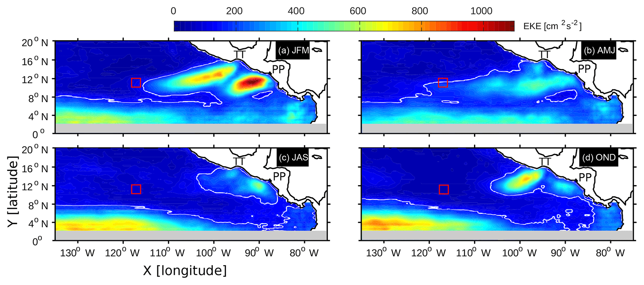
Figure 1Spatial distribution of seasonal mean eddy kinetic energy (EKE) over a period from 1993 to 2016 obtained from AVISO satellite altimetry data for (a) January–February–March, (b) April–May–June, (c) July–August–September, and (d) October–November–December. The solid white contours represent an EKE of 150 cm2 s−2, which is assumed as a threshold for highly energetic regions. The red square indicates the location of the study region (abbreviated as SR in the text).
The eddy kinetic energy (EKE) as a measure of mesoscale eddy activity is calculated from SSHAs derived from high-pass-filtered satellite products as follows:
where and are deviations from monthly mean geostrophic velocities, which are computed from SSHA gradients as
where g is the gravitational acceleration, f is the Coriolis parameter, and x and y are the eastward and northward distances (Stammer, 1997). Note that the SSHA and EKE include low-frequency variability, seasonal cycles, and mesoscale eddies; however, the eddy detection algorithm ensures through limitations that the detected eddies are mesoscale. The spatial distribution of mean seasonal EKE constructed from the 24-year SSHA data in the NETP for the time period between 1993 and 2016 is shown in Fig. 1.
In addition to the region of the North Equatorial Countercurrent (south of 6∘ N), where the EKE permanently shows values higher than 500 cm2 s−2, a greatly elevated EKE signal is located in the region of the gap winds off the coast of Mexico, albeit with a strong seasonal variability. An EKE with values larger than 700 cm2 s−2 is found in autumn and winter, when strong gap wind events initiate ageostrophic ocean currents (see Fig. 1a–d). In the spring season (Fig. 1b), the EKE reduces to values of about 400 cm2 s−2 in the Tehuantepec (TT) and Papagayo (PP) gulfs. In summer, the intensity and occurrence of northerly winds in the TT gap wind region are reduced (Romero-Centeno et al., 2003); thus the EKE drops to values below 300 cm2 s−2, and its effect on the background EKE of the ocean is restricted to a much smaller region (see the white contours in Fig. 1c). A comparison of seasonal variation in EKE in the NETP reveals an interesting feature. Despite the lower amount of EKE in April–June, with no significant peak, the energetic region is pushed further offshore in this period (see the position of the white solid line in Fig. 1). A biseasonal variation in EKE in the region of the PP and TT gap winds in summer and autumn is also evident. The summer peak in EKE in the PP gap wind region is due to an increase in easterly winds during August in this region (Romero-Centeno et al., 2003).

Figure 2An example for applying the eddy detection algorithm on sea surface height altimetry data for 31 January 2016. Detected eddies are shown as closed black contours. The associated geostrophic field is shown by the black arrows. Cyclonic and anticyclonic eddies can be identified as differences in direction of water mass rotations. Centers of eddies are indicated as the black stars for each individual vortex. The amplitude of sea surface height is color-coded.
3.2 Eddy detection, numbers, and lifetimes
An example of the application of the eddy detection algorithm on SSHA data is shown in Fig. 2. On 31 January 2016, 15 eddies with different sizes, strengths, and shapes are shown as closed black contours. Sea level height and associated geostrophic currents are shown in the background throughout the entire studied region (NETP). The center of each eddy, which is defined as the location with minimum local velocity, is depicted as a black star. The current fields are shown by the arrows, and the direction of current rotation reveals the polarity of eddies.
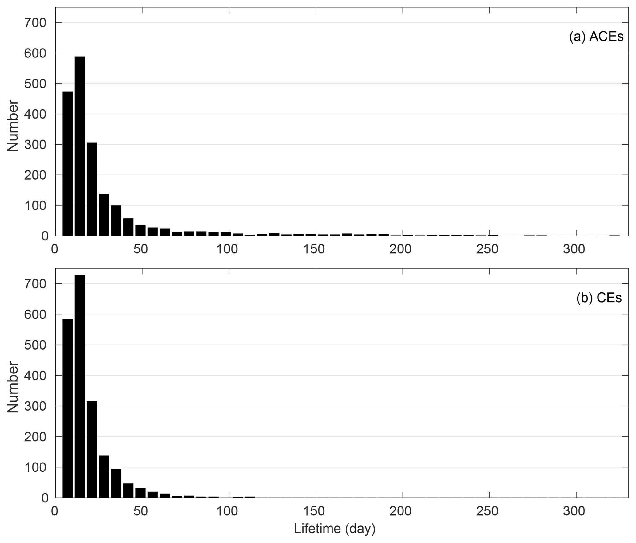
Figure 3Number of (a) anticyclonic eddies (ACEs) and (b) cyclonic eddies (CEs) from 1993 to 2016, plotted as a function of their lifetime. Eddies with lifetimes shorter than 7 d were excluded from the analysis. The bin width for eddy lifetime is 7 d.
Applying the eddy detection geometry algorithm to the long-term SSHA data from 1993 to 2016 in the NETP enables us to extract some important information on characteristic eddy parameters such as abundance, size, lifetime, polarity, translation, and swirl velocity. Any eddy that satisfies the eddy detection algorithm attributes and lasts for longer than 2 d is counted as a significant eddy in our analysis. An eddy is not counted at each time step of its lifetime but is dealt with as a single eddy (for its entire lifetime) from the time of formation until its decay. In total, 6202 cyclonic eddies (CEs) and 5363 anticyclonic eddies (ACEs) were detected. This can be translated to a mean annual number of 258 CEs and 223 ACEs in this region. Thus, the total number of CEs exceeds the ACEs by about 16 %. It should be noted, however, that the number of detected eddies very much depends on the arbitrary parameters defined earlier in Sect. 2. Most of the detected eddies have a lifetime shorter than 7 d. Figure 3 shows the distribution of eddy abundance when eddies with lifetimes shorter than 7 d are excluded. ACEs with lifetimes longer than 50 d occur frequently, whereas CEs with such lifetimes are uncommon. Eddies of both types have peak lifetimes of around 14 d. The average lifetimes of CEs and ACEs over the period of our study are 18 and 28 d, respectively, meaning that ACEs last almost 50 % longer in the ocean than CEs. The average lifetime of ACEs detected in the NETP is of the same order as those described from the southeastern Pacific Ocean (Chaigneau et al., 2008), although the lifetime of CEs in the NETP is shorter than CEs in that region. Eddy analysis in the subtropical zonal band of the northern Pacific Ocean (Liu et al., 2012) has revealed much longer eddy lifetimes, resulting from the instability of the Kuroshio current. Though in the same basin of the Pacific Ocean, Dong et al. (2012) show that eddies in the Southern California Bight have relatively short lifetimes, with an average lifetime of 5–14 d, comparing well to our results. Varying origins, advection processes, and decaying factors might be the reason for the different eddy lifetimes observed in the various basins of the Pacific Ocean.
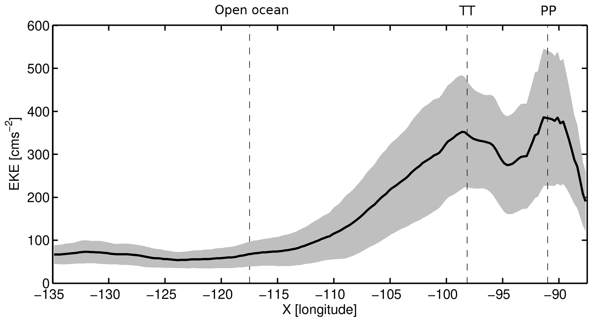
Figure 4Zonal variability of meridionally averaged EKE between 9 and 16∘ N. The values are then averaged over the period of study, from 1993 to 2016. The shaded area shows the ± 0.5 SD, averaged over the whole period at each position. The dashed lines show the EKE of the ocean circulation in the open ocean and two local maxima driven by TT and PP gap winds, respectively. The continental shelf is on the right side of the figure.
3.3 Spatial distribution of eddies
Identifying regions of eddy genesis and high eddy abundance is important for understanding eddy lifetimes and trajectories. The zonal variability of meridionally averaged EKE over the entire period of 24 years between 9 and 16∘ N is shown in Fig. 4. The figure shows that regions with high EKE are restricted to the continental shelf, with a rapid decrease towards EKE values in the open ocean. Two significant peaks are observed in the EKE values, which correspond geographically to the zonal location of the Tehuantepec and Papagayo gap winds. These are thus hotspots for eddy genesis. No eddy formation hotspot is found offshore. Moreover, west of 110∘ W, the EKE and its variation are reduced by a factor of 5, showing that the energy level in the open ocean cannot be satisfactorily explained by offshore eddy formation. As eddies propagate into the open ocean, they encounter the East Pacific Rise (EPR) at ca. 105∘ W. The EPR is a long, north-to-south-oriented midocean ridge system whose height is about 1200 m shallower than the surrounding seafloor. The rapid drop in EKE west of 105∘ W is most likely caused by this topographic feature (Palacios and Bograd, 2005).

Figure 5Spatial distribution of the probability of eddy occurrence in bins of resolution for (a) anticyclonic eddies (ACEs) and (b) cyclonic eddies (CEs).
In order to further explore the spatial distribution of eddies in the NETP, the probability of eddy occurrence (CE vs. ACE) was calculated using the available data from 1993 to 2016, with a horizontal resolution of 1∘ (Fig. 5a and b). The probability of eddy occurrence is defined at each cell as the percentage of time that the cell is located within a vortex. The eddy probability ranges between 0 % and 68 % for anticyclonic and 0 % and 62 % for cyclonic eddies. The coastal regions close to the gap winds show the highest probability for both types of eddies, with values larger than 30 % (compare the number of cells with the high probability in Fig. 5a and b). Moreover, the region with high eddy probability for ACEs is extended far offshore west of 100∘ W, while for CEs the region of high eddy probability is limited to the east of 100∘ W.
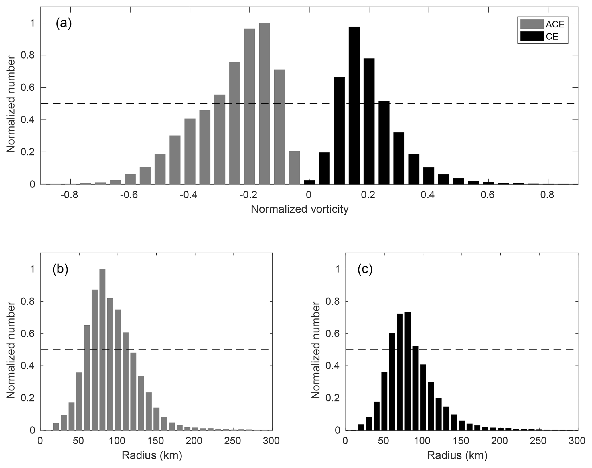
Figure 6(a) Histogram of eddy vorticity for eddies with a lifetime longer than 7 d for the time interval between 1993 and 2016 with a bin width of 0.05. Cyclonic eddies (CEs) and anticyclonic eddies (ACEs) are mirrored for better visualization. The eddy vorticity is normalized to the local Coriolis parameter. (b) Histogram of eddy radius for anticyclonic eddies with lifetimes longer than 7 d during the time interval from 1993 to 2016. (c) Histogram of eddy radius for cyclonic eddies with lifetimes longer than 7 d during the time interval from 1993 to 2016. The number of eddies has been normalized to the maximum number of anticyclonic eddies (736 ACEs with a radius of 80 km). The thick gray line depicts a normalized number of 0.5.
3.4 Eddy vorticity and radius
We define the vertical relative vorticity () of an eddy at its center. A histogram of the relative vorticities for cyclonic and anticyclonic eddies with lifetimes longer than 7 d is shown in Fig. 6a. Generally, ACEs have higher absolute values of relative vorticity than CEs. The peak of absolute vorticity for both types of eddies is between 1.5 × 10⁻⁶ and 2 × 10⁻⁶ s−1 but with stronger asymmetries towards eddies with higher vorticities for ACEs. The normalized distribution of ACEs is more skewed to the larger vorticities compared to the CEs. The mean vorticity of all ACEs for the entire period of time (−0.26 × 10⁻⁵ s−1) also has a larger magnitude than that for all CEs (0.2 × 10⁻⁵ s−1).
As anticyclonic eddies move westward from the coast of Mexico, they encounter the East Pacific Rise, with a change in seafloor depth from 4000 to 2800 m. In order to conserve the potential vorticity as the depth decreases, the absolute vorticity (ζ+f) must also decrease. Therefore, eddies with strong intensity deviate toward the Equator and lose their planetary vorticity. Our analysis shows that the relative vorticity of ACEs for each degree of meridional displacement reduces by a factor of 3.5 × 10⁻⁶. For the weaker eddies that do not have enough energy to move equatorward, the topographic blocking might be the main reason for decay of eddies due to the combined effects of reduced relative vorticity and increased frictional dissipation of eddy kinetic energy caused by the elevated seafloor.
As eddies are not necessarily circular in shape, an eddy radius is defined as , where A is the area delimited by the eddy's edges.
Understanding the size of eddies in the ocean can help us to analyze the eddy intensity and determine their impact on the open ocean. Histograms of eddy radius distribution for CEs and ACEs with lifetimes longer than 7 d during the time interval between 1993 and 2016 are shown in Fig. 6b and c. The number of eddies of each type is normalized to the maximum abundance accordingly.
A non-Gaussian distribution of eddy radius with strong asymmetries is observed for both types of eddies. The radius of ACEs with a normalized number higher than 0.5 (shown by the dashed black line in Fig. 6b) shows a wide range, from 60 to 110 km. In contrast, CEs are limited to a radius between 60 and 90 km.
A high number of ACEs have radii between 60 and 110 km. Eddies of both types with a large radius (> 150 km) are infrequent but cannot be neglected. The temporal mean eddy radius between 1993 to 2016 for ACEs is 92 km, whereas CEs have a smaller mean radius of 84.5 km. Further analysis on the radius of ACEs obtained from year to year between 1993 and 2016 shows only a small long-term variation in eddy size. The small changes in long-term SD of eddy radius (32 km ± 2.5 km) illustrate that decadal climate variability has a negligible impact on eddy size in this region. However, the large value of mean annual SD of eddy radius (32 km) indicates inhomogeneity in the size of eddies, reflecting a strong seasonality in eddy formation in this region.
Besides the seasonal variability in the size of eddies, the analysis of spatial distribution of eddy radius in this region shows that the size of eddies increases with decreasing latitude. This is associated with the baroclinic Rossby deformation radius changing with latitude, from 60 km at 20∘ N to 150 km at 6∘ N (Chelton et al., 1998).
3.5 Translation speed and swirl velocity of eddies
The average translation velocity of an eddy is determined by considering the distance between the location of eddy generation and eddy degeneration and the time traveled by the eddy. Significant differences are found between the averaged translation velocities of ACEs and CEs. The analysis of all ACEs with lifetimes longer than 7 d indicates that the average translation speed of ACEs is 12.5 cm s−1, with a minimum and maximum speed of 3.4 and 18.1 cm s−1, respectively. The high translation velocity of ACEs is attributed to the large southward velocity component of eddies. In contrast, CEs show notably slower translation speeds, varying between 4.1 and 10.7 cm s−1, with a mean translation speed of 6.8 cm s−1.
Previous analyses of eddy translation speeds in the zonal band of the North Pacific Ocean (Liu et al., 2012) and in the Chile–Peru basin (Chaigneau et al., 2008; Stramma et al., 2014) indicate a lower mean translation speed of 4–7 cm s−1 for ACEs and CEs, with almost no difference between the two eddy types. Therefore, the higher mean eddy translation velocity found for ACEs in this region can be considered as a specific characteristic of eddies in the NETP. The mean translation speed of CEs in the NETP is very similar to those reported in previous studies mentioned above.
The average surface swirling velocities (Vθ) of the eddies increase outward and reach values of around 25 cm s−1 and 10 cm s−1 at the outer boundaries of the eddies for ACEs and CEs, respectively. The higher average swirl velocity of ACEs might be also a reason for their longer lifetime in the ocean. The nonlinearity parameter of eddies, which is characterized by the ratio of swirl velocity to translation velocity (Vθ∕VT), was calculated. Most of the eddies of both types in this region indicate a significant degree of nonlinearity (), implying that eddies can maintain a coherent structure, which may isolate the interior water mass, without interaction with ambient water while propagating in the ocean. Similar to previous studies (Stramma et al., 2014; Czeschel et al., 2018) in the South Pacific Ocean, the activity of nonlinear long-lived eddies may result in a large-scale anomalous water mass distribution in this region.
3.6 Trajectory of long-lived eddies
We consider eddies with lifetimes equal to or longer than 90 d to be long-lived eddies. From 1993 to 2016, 106 long-lived ACEs and only 7 CEs were detected in this region. The number of long-lived ACEs substantially exceeds the CEs detected in the NETP, which is different from the distribution of eddy abundance when all eddies longer than 1 d were considered (see Sect. 3.2).
The number of long-lived CEs present a challenge to our statistical analysis, and therefore they were removed from our trajectory analyses. The trajectories of ACEs with a lifetime longer than 90 d are shown in Fig. 7. To ease the comparison, eddies are divided into different lifetime classes between 91 and 321 d, with a time interval of 37 d.
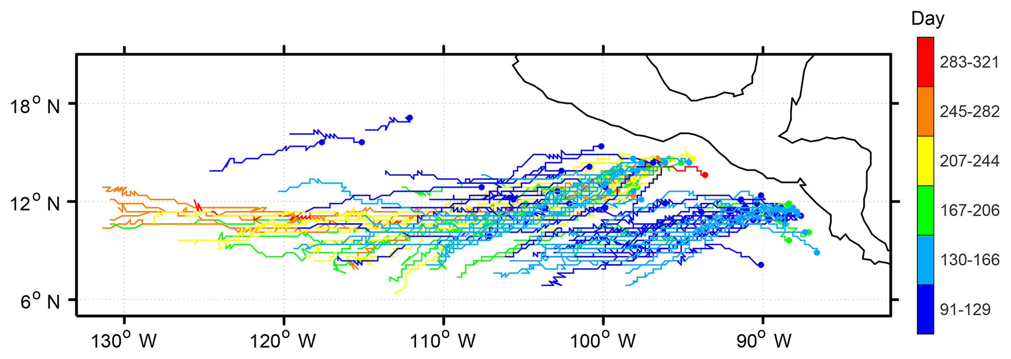
Figure 7Trajectories of long-lived anticyclonic eddies (ACEs) with a lifetime equal to or longer than 90 d during the time interval from 1993 to 2016. The lifetimes of detected eddies are divided into six classes. Tracks of eddies are shown in colors corresponding to each lifetime class.
Table 1Mean distance traveled, mean translation velocity, and number of long-lived ACEs per age class as shown in Fig. 7.
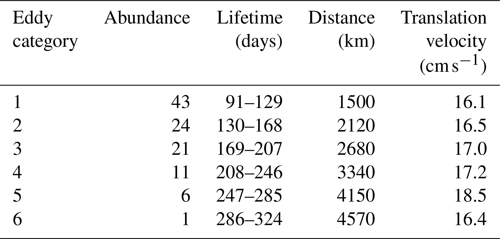
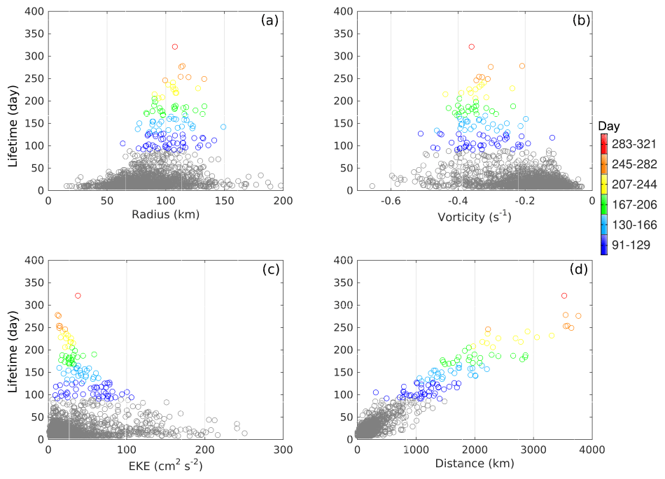
Figure 8Relationships between eddy lifetime and (a) eddy radius, (b) eddy vorticity, (c) EKE, and (d) propagation distance into the ocean for all anticyclonic eddies with lifetimes longer than or equal to 7 d. Long-lived eddies are shown using the color scheme as used in Fig. 7. Eddies with lifetimes shorter than 90 d are depicted as gray circles. Note that each circle represents the mean value of every parameter throughout its life period against the eddy lifetime.
The number of ACEs with lifetimes between 91 and 129 d almost equally derive from both the Tehuantepec (TT) and Papagayo (PP) gap wind regions, with a slightly larger number of eddies formed in PP than in TT. The number of eddies formed in the TT and PP gap wind regions for the next two lifetime classes, 130–166 and 167–206 d, do not show significant differences. For the eddies with lifetimes longer than 207 d (eddies depicted by yellow, orange, and red colors in Fig. 7), the eddy generation region is different, with all eddies originating in the TT gap wind region. The genesis of long-lived eddies in the TT gap wind region is consistent with the more energetic Tehuantepec jet winds (both in magnitude and duration) compared to the Papagayo jet winds (McCreary et al., 1989; Chelton et al., 2000; Romero-Centeno et al., 2003).
Long-lived eddies have a preferred range of eddy size. Neither small nor very large eddies last long in the ocean, and they dissipate due to their low intensity (Fig. 8a). Most of the long-lived eddies have a vorticity range between 0.2 × 10⁻⁵ s−1 and 0.4 × 10⁻⁵ s−1 and a radius between 60 and 150 km (Fig. 8a and b). An inverse relationship between eddy size and eddy vorticity particularly for long-lived eddies is found. The eddy size appears to decrease when the vorticity of long-lived eddies increases.
In most cases, long-lived eddies travel for a distance of more than 1000 km into the interior ocean (Table 1). In fact, long-lived eddies generated in the TT gap wind region can travel a distance of about 4500 km, which is almost twice as far as the travel distance observed for eddies that originate in the PP gap wind region (Fig. 7). Furthermore, except for the eddy category 6, which is the longest-lived eddy observed in the studied region, the mean translation velocity of eddies increases with lifetime (Table 1).
3.7 Interannual variability of eddy parameters
In the eastern Pacific Ocean, the El Niño–Southern Oscillation (ENSO) is the most dominant climate mode on interannual timescales, and this could well have an effect on the variability of eddy characteristics in the NETP. To remove effects of seasonal fluctuations on eddy properties, the annual mean of each characteristic eddy parameter was compared with the Oceanic Niño 3.4 Index (ONI) for the time period under consideration (1993–2016). The study period has clear phases of warm (cold) events associated with El Niño (La Niña) cycles.
Figure 9a shows the relationship between the ocean EKE in the TT and PP gap wind regions and the ONI. The EKE of the ocean in the PP appears to be strongly related to the ONI and thus to large-scale climate variability. These findings are confirmed by sea surface temperature anomalies in the gap wind regions (Alexander et al., 2012). The amount of wind energy induced to the ocean in the PP increases during warm episodes of the ENSO cycles due to equatorward movement of the Intertropical Convergence Zone (ITCZ), which enhances the positive wind curl on the southern flank of the PP wind jet (Karnauskas et al., 2008).
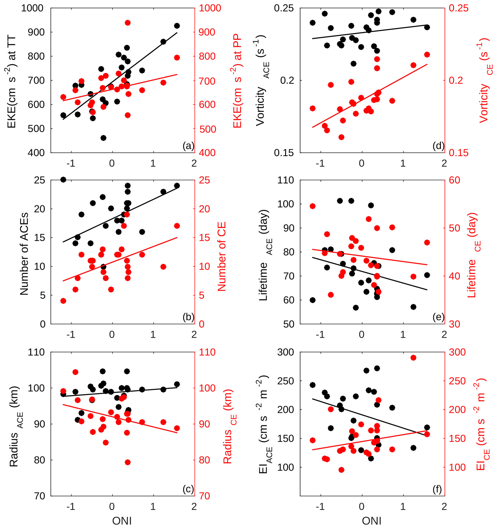
Figure 9Relationship between the Ocean Niño Index (ONI) based on the Oceanic Niño 3.4 Index and (a) EKE in the TT and PP gap wind regions, (b) number of eddies, (c) radius of eddies, (d) vorticity of eddies, (e) lifetime of eddies, and (f) intensity of eddies, all with lifetimes longer than 28 d. The black and red dots in (a) refer to EKE in the TT and PP, and in (b–f) they refer to eddy characteristics of ACEs and CEs, respectively. The best fits for the scatterplots are shown as solid red and black lines. EKE values used in (a) correspond to areas with an EKE value larger than the average EKE throughout the period 1993 to 2016.
The impact of ENSO events on the intensity and frequency of northerly winds in the TT is more complicated and has been addressed in previous studies (e.g., Romero-Centeno et al., 2003; Zamudio et al., 2006). In contrast to the La Niña years, during which winds are significantly weaker, and the occurrence of northerly winds is significantly rarer, during El Niño years the more frequent occurrence of strong northerly winds is restricted only to May and September. This can be further demonstrated by comparing chlorophyll a (CHL) concentration in TT and PP gap winds during the famous 1997–1998 El Niño, during which the wind stress was weaker (see Figure 5 in McClain et al., 2002). The lower level of CHL concentration in the PP shows a strong relation with weaker wind stress. No correlation between these two parameters in the TT gulf confirms the weaker influence of El Niño on TT gap winds.
The number of eddies, both for ACEs and CEs, shows a clear but weak positive relationship to the ONI (Fig. 9b). Strong La Niña events (ONI < −0.5) apparently induce a decline in the number of eddies of both types. An increase in the number of eddies was evident for the case of strong El Niño events (ONI > 0.5). The effect of weaker ENSO cycles, with −0.5 < ONI < 0.5, on the variability of eddy number is more complicated and does not show a clear trend. Despite the lack of a significant increase in suitable winds for mesoscale eddy formation in the TT during El Niño years, a larger number of mesoscale eddies in agreement with our results is reported in this region in previous studies (Zamudio et al., 2001, 2006; Palacios and Bograd, 2005). Thus, in contrast to the initial hypothesis, eddy formation and its interannual variability in the TT region cannot be solely explained by strong and intermittent wind events. The analysis of a high-resolution ocean model forced by European Centre for Medium-Range Weather Forecasts (ECMWF) meteorological data from this region shows that an increase in propagating, downwelling, coastally trapped waves (CTWs) during El Niño years plays a crucial role in the modulation and generation of TT eddies (Zamudio et al., 2006). While the CTWs propagate along the coast of Central America and Mexico, a strong horizontal and vertical shear of the horizontal velocity is generated, which can trigger barotropic and baroclinic instabilities. The breaking of long-wavelength CTW meanders generates mesoscale eddies in this region (Zamudio et al., 2006).
The relationship between size and interannual climate variability is different to that of eddy number. The correlation analysis shows a negative dependency of −0.41 between the radius of CEs and the ONI. This means that during La Niña (El Niño) events, larger (smaller) CEs are generated in the ocean. The very weak correlation between the radius of ACEs and the ONI (0.21) implies no meaningful relationship in this case.
The eddy vorticity of CEs has been found to follow the ENSO variability, with a positive and significant correlation of around 0.7. During a strong La Niña period, the vorticity of CEs decreases to the lowest value (Fig. 9d). Eddy vorticity reaches its peak value during strong El Niño phases. This may explain the inverse relationship of the ONI and the size of CEs, assuming the conservation of angular momentum for a vortex in the ocean.
The correlation of eddy lifetimes and the ONI shows a negligible (−0.15) and a weak (−0.25) relationship, respectively for CEs and ACEs, which in both cases are inverse (Fig. 9e). This may indicate that ACEs live longer during La Niña phases, while a strong El Niño event does not have a significant impact on the lifetime of ACEs in the ocean.
The eddy intensity (EI), which is calculated as the mean EKE over the vortex area, shows a different behavior for eddies with distinct polarity. Although the CEs show a moderate positive correlation (0.44) with ENSO cycles, the intensity of ACEs demonstrates a negative low relationship with the ONI. This means that the highest intensity of ACEs (CEs) takes place when strong La Niña (El Niño) events develop (Fig. 9f).
In summary, the strength and direction of the relationship between the ONI and characteristic parameters of mesoscale eddies of both types illustrate that ENSO cycles have a profound effect on their development in the NETP.
4.1 Lag response of ocean bottom current properties to an anticyclonic surface mesoscale eddy
Large eddies passing through the open ocean can have a profound effect on the variability of near-bottom currents even at depths of 4000 m or more (e.g., Demidova et al., 1993; Kontor and Sokov, 1994; Liang and Thurnherr, 2012; Zhang et al., 2014; Aleynik et al., 2017). To illustrate the response of the deep-ocean environment to ocean surface mesoscale eddies, we look at the changes in current properties from 19 March to 2 June 2015 in the vicinity of the seafloor while an anticyclone eddy passes through the study region (SR; Fig. 10).
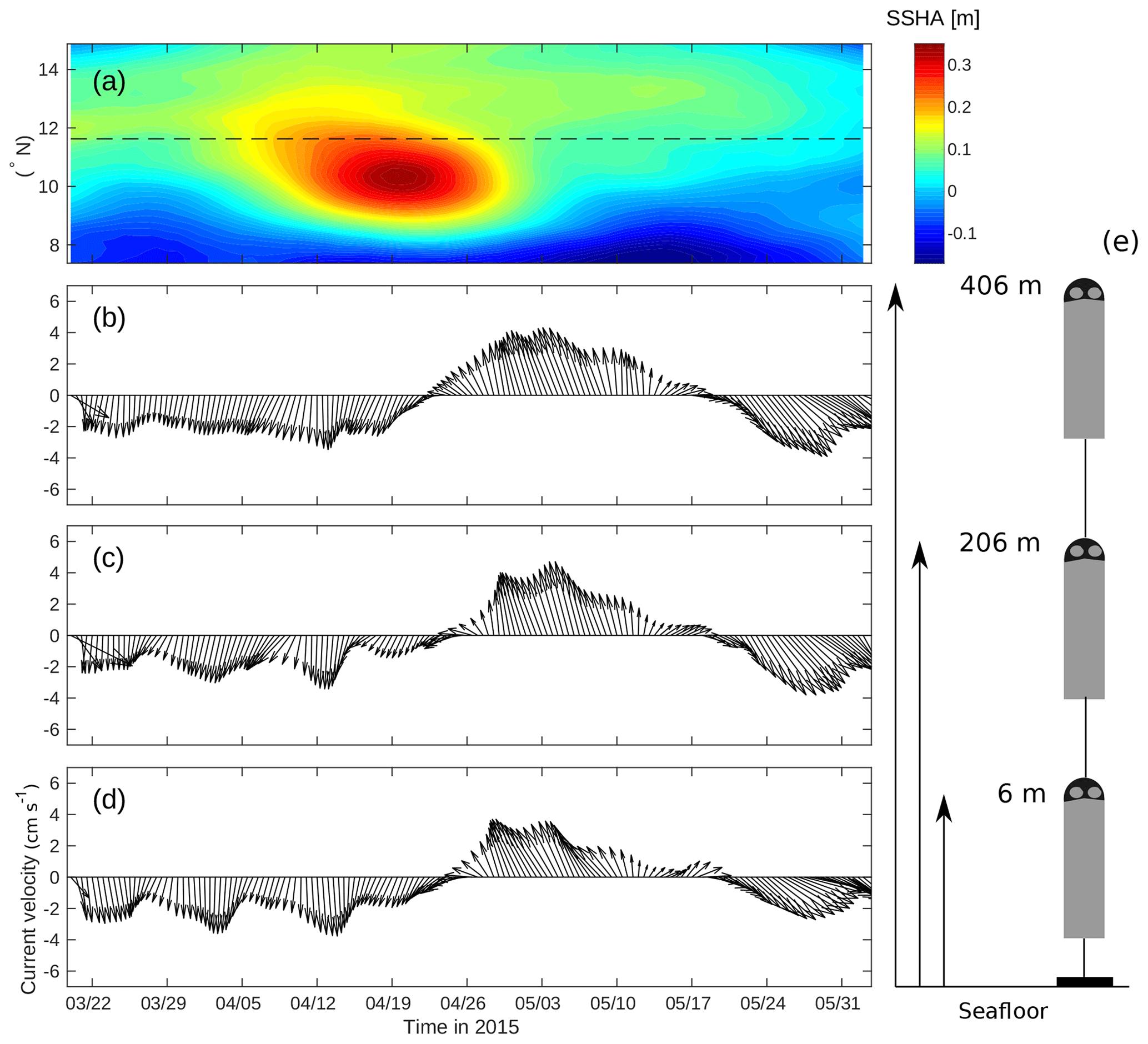
Figure 10(a) Temporal evolution of the SSHA at a zonal transect in the SR from 7∘ to 15∘ N from 20 March to 2 July 2015. Ocean current velocity recorded by an array of single-point Aquadopp current meters at 406 m above the seafloor (b), at 206 m above the seafloor (c), and at 6 m above the seafloor (d). These heights above the seafloor correspond to 3788, 3971, and 4180 m water depth. (e) A schematic figure of the current meter array. The dashed black line in (a) shows the latitude where the geographical center of the moorings is located. All current velocities are averaged over a half-day period and shown here.
An anticyclonic long-lived eddy with an average radius of 130 km was tracked from its genesis in the TT region on 14 October 2014 using the automated eddy-tracking algorithm. This mesoscale eddy traveled a distance of about 2580 km in the ocean interior with an average translation velocity of 13.8 cm s−1 and passed south of the observation array moored in the SR while collecting oceanographic data in the potential region for future DSM (see Fig. 10e).
The outer edges of the anticyclonic eddy with positive sea surface height anomalies higher than 10 cm reach the SR on 5 April 2015. The ocean currents tilt in to a northward direction on 22 and 25 April at 406 m and 6 m above the seafloor, respectively. As the eddy approaches the location of the mooring, the current direction reaches its consistent northward direction in early May. The clear impact of surface anticyclonic eddies is found in the deep layer of the ocean, with a strong rotation of the dominant current direction from south to the north at all layers. The northward changes in current direction fit well with the clockwise rotation of anticyclonic eddies. The impact of the maximum SSHA that occurs on 19 April is observed when the current velocities reach their maximum strength, and the current direction shows a strong deviation from its dominant southward direction. The slightly stronger northward currents continuously last for 3 weeks until 18 May, and the current direction returns to the main southward direction afterward (see current direction after 20 May at Fig. 10b–d). The impact of the observed eddy is more attributed to the rotation of the dominant current direction than to current intensification. Nevertheless, the current velocities show values slightly larger than 4.5 cm s−1 for a period of 4 weeks at the upper layers (compare Fig. 10b–d). The weak intensification observed in current velocity during May 2015 is due to the large distance of the eddy center, which is about 1∘ away from the current meter array to the south, which reduces the eddy impact on current velocity intensification. The lag times for changes in current velocity and direction observed in our measurements are consistent with the interactions of hydrodynamic processes caused by the surface eddies.
Comparing the current magnitude at different depths shows a declining tendency, suggesting that the feedback of the deep ocean to the surface eddies is attenuated with increasing depth. However, as indicated here, the eddy-induced hydrodynamic influence on the observed near-bottom ocean current characteristics lasted for 1 month, and it can be assumed that similar modulations of current properties can be seen for the entire water column.
The impact of surface eddies on deep-sea current velocities in the NETP has been addressed earlier by Adams et al. (2006). The current velocities measured at a depth of 2430 m from May to June 2007 at 9∘50.0 N, 104∘17.4 W show deep-sea current velocity exceeding 15 cm s−1 during the sea surface height anomaly, which is almost 3 times faster compared with the mean current speed of 5.5 cm s−1 in this region. The stronger current velocities observed in this study as compared to our measurements are likely due to the more significant impact of eddies on the deep sea due to the shorter distance of the eddy center from the mooring arrays, while our moorings are located at a distance of almost 100 km away from the eddy center. Besides, the larger EKE of the young eddies and the shallower water depth in this region could be another reason for larger deep-sea current velocities. Due to the geographical location of the observations in their study, eddies in their stable life stage with relatively larger EKE content reach this region first. The shallower water depth in this region may also cause less energy dissipation in the ocean layers, and thus currents in the deep sea contain greater EKE.
The lagging feature of deep-ocean current response to the passage of a surface eddy observed in this region is similar to the results showed by Zhang et al. (2014) in the South China Sea (SCS), where they found a lag of 12 d between current velocities at the deep layer and the surface geostrophic velocity. The longer time lag observed by Zhang et al. (2014) can be related to the different water column stratification in the SCS. These authors also showed that there are longer lags between the observed near-bottom suspended-sediment concentration and surface geostrophic velocities. Adams et al. (2006) also found that near-bottom current intensification lags the surface height anomalies by 8 d. Considering the water depth of approximately 2400 m in this study and 4100 m in the SR, the longer time lag of 15 d between surface anomalies and the observed responses of the deep sea in our measurements is shown to be linearly related to the water depth.
Despite some general similarities in the responses of deep-sea to surface mesoscale eddies in the SCS and observed eddies in the SR, the lagging response and current magnitude intensifications are different. The different lagging response of bottom current properties to passing surface mesoscale eddies can be mainly attributed to the different water depth and vertical stratification in the two basins. The measurements in the SCS are taken at a water depth of 2600 m, which causes a faster transfer of EKE to the deeper layers in this region. Moreover, the slower translation speed of ACEs in the SCS (10 cm s−1) more likely causes higher energy uptake by the deeper layer of ocean and results in a significant current intensification in the SCS.
With respect to the hydrographic response of the deep ocean to the mesoscale surface eddies, several studies have shown that sediments in deep oceanic basins may be actively resuspended and redistributed where the bottom current regime is significantly enhanced due to eddy activity (Gardner and Sullivan, 1981; McCave, 1986; Isley et al., 1990). In the Gulf of Lions, episodes of local sediment resuspension appear to occur for current speeds between 17 and 30 cm s−1 (Durrieu de Madron et al., 2017). Moreover, Gardner et al. (2017) showed that minimum current speeds required to resuspend material from the local seabed in the western North Atlantic Ocean are likely in the range of 10–20 cm s−1, which is observed to happen often and closely matches with deep high-EKE episodes. The eddy-induced current velocities observed between April and May 2015 in the CCZ region reached only 5–6 cm s−1. This is below the required bottom current velocities of 9–12 cm s−1 observed in laboratory experiments by Gillard et al. (2019) with local sediment from the German license area in the CCZ. The optical sensors attached to the OBM did not record an increase in turbidity level while the surface mesoscale eddies passed the location of the moorings. Hence, the observed eddy-induced bottom current velocity at the bottom was not strong enough to resuspend naturally deposited deep-sea sediment in the investigated CCZ region. However, it can be assumed that freshly redeposited sediment from a mining-generated plume most likely requires lower shear stress at the seabed for resuspension, which might be achieved even by the low-EKE bottom regime driven by a weak surface mesoscale eddy.
Our short-term observation suggests that eddy-driven impacts not only extend into the deep-sea benthic environment but also – depending on the eddy strength, eddy track, and seawater hydrographic condition – can modulate the hydrodynamics of the deep-ocean environment, which plays a vital role in the distribution of suspended sediment plumes from mining activities and their redeposition on the seafloor. Stronger bottom currents will inevitably drastically enlarge the spatial footprint of the mining-induced sediment plume; however, sediment concentrations will decrease due to the increased dispersion. As a consequence, the resettled sediment blanket on the seafloor, adjacent to the mined area, will become thinner and more extended. Hence, eddies will strongly alter the expected spatial footprint and severeness of the environmental impact. A key parameter for assessing the environmental impact of sediment plumes is the EKE.
4.2 Long-term ocean current variability and its relationship to EKE in the region of gap winds
In this section we aim to assess the importance and linkage of sea surface mesoscale eddies which are generated in the vicinity of the gap winds to the annual variability of deep-ocean current properties in the SR. A combination of relatively long-term deep-ocean current measurements (3 years, between 2013 and 2016) in the SR, merged satellite SSHA data, and an eddy-resolving global ocean reanalysis product is employed.
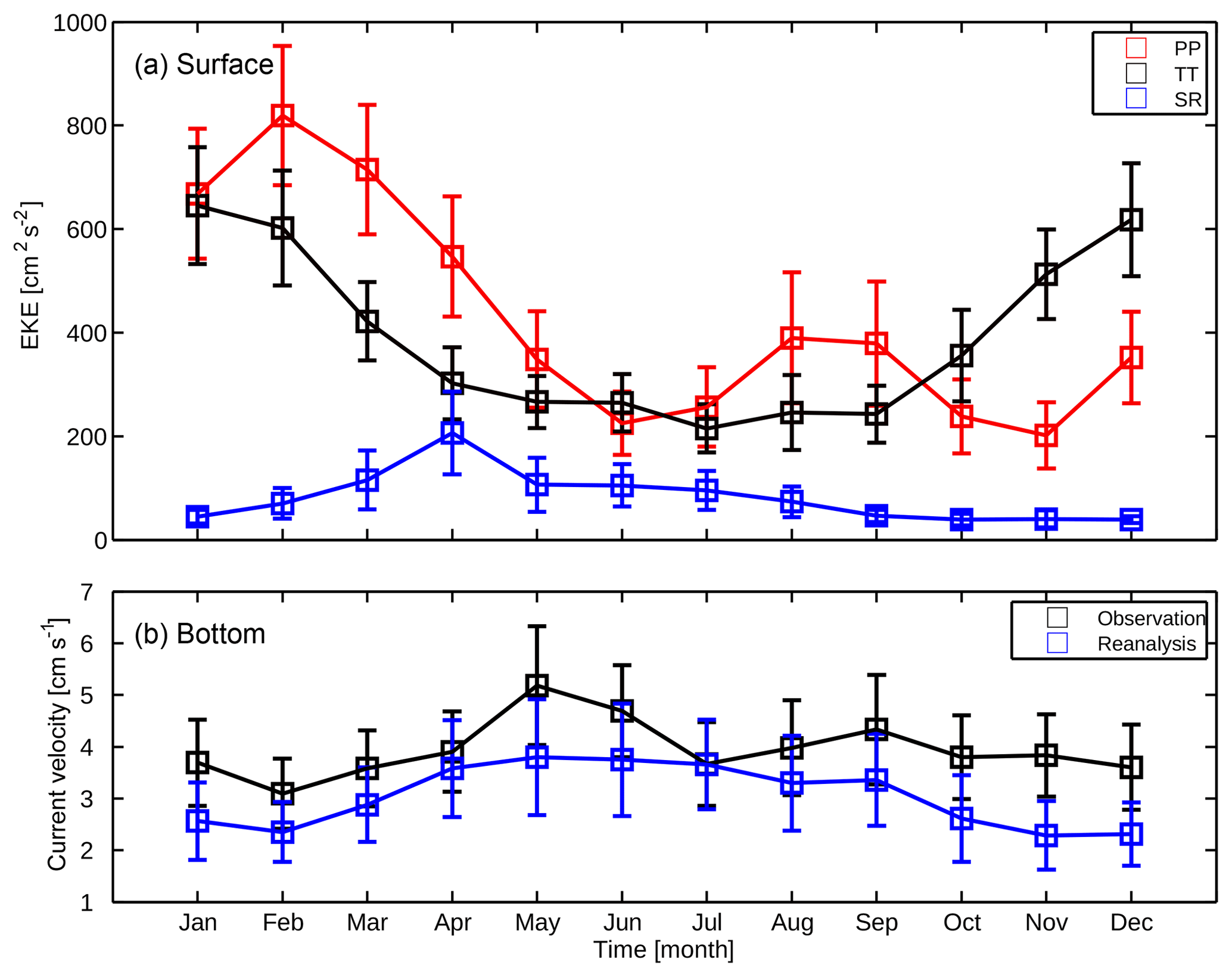
Figure 11(a) Annual cycle of monthly mean sea surface EKE, averaged over 24 years for the Papagayo (PP) gap wind region (averaged over 10.5–12.5∘ N, 93.5–88.5∘ W), the Tehuantepec (TT) gap wind region (averaged over 12.5–14.5∘ N, 100–95∘ W), and the offshore study region (SR; averaged over 10.5–12.5∘ N, 118–116∘ W). (b) Monthly averaged current magnitude (black line) at the seafloor of the SR from April 2013 until May 2016, obtained from three moored ADCPs. The blue line represents the same but with data obtained from the reanalysis model and averaged from 1993 to 2016. SD with a 95 % confidence level is shown as error bars. The error bars have been reduced to half of their size to avoid overlapping.
To investigate the interaction between the EKE in the region of the gap winds and in the SR approximately 2500 km away from the coast, we computed the long-term monthly mean EKE, averaged over 24 years in both regions. The impact of high-frequency wind events on the variation in EKE at the study site is limited to the period between late autumn and early spring, when higher EKEs extended into the ocean interior (Fig. 1b). A pronounced seasonal variability of EKE in the TT and PP regions is observed, with slightly different timing despite the close geographical location of TT and PP (Fig. 11a). This is due to the different mechanisms of wind generation and its development in these regions. The monthly mean EKE in the PP gap wind region is generally higher, with a maximum in the winter (> 800 cm2 s−2). A second maximum occurs in August, which is related to a local increase in wind velocity (Romero-Centeno et al., 2003). The level of EKE in the TT region is marginally lower, with an increase starting in November that lasts until the end of February (Fig. 11a). Strong seasonality in surface EKE at the ocean interior is also observed, although with a different timing (see the blue line in Fig. 11a). Here, an absolute maximum value of EKE occurs between April and June.
Unlike most of the eddies formed in the PP gap wind region, which are observed to dissipate before they reach west of 110∘ W, most of the long-lived eddies with an origin close to the TT region travel long distances into the ocean interior (see Fig. 7). Therefore, the variability of EKE in the ocean interior is suggested to be more susceptible to alteration by eddies originating from the TT region. The cross-correlation analysis of the daily EKE time series in the TT and SR regions indicates a significant correlation of 83 %, with a time lag of 165 d. To test the hypothesis of no correlation, the P values are calculated. All the P values for the Pearson correlation coefficients of EKE in the TT and SR are too small, indicating a significant correlation. The time lag between EKE in gap winds and EKE in the SR is now consistent with the required time for a long-lived ACE, with an average translation velocity of 16.9 cm s−1 (see Table 1) to travel a distance of 2400 km from TT gap winds to the SR region. However, no significant correlation between EKE in the PP region and the far offshore region was obtained.
Therefore, we conclude that the observed seasonal variability of EKE in the open ocean is primarily driven by the eddy-dependent anomalous transport of EKE originating from the TT gap wind region.
To illustrate the relationship between passing surface eddies in the ocean interior and deep-ocean current characteristics close to the seafloor at a water depth of 4100 m, monthly mean deep-sea current speed obtained from the three OBMs over a period of 3 years, from April 2013 to May 2016, was calculated (black line in Fig. 11b). The qualitative feature of EKE seasonality at the ocean surface is transferred through the entire water column to the bottom of the ocean with a time lag of about 1 month. More intense current velocities with higher variability are observed between April and September at the seafloor (Fig. 11b). The average monthly current velocity reaches its maximum value of 5.8 cm s−1 in May, indicating an increase in current velocity from the mean value of 3.9 cm s−1 of almost 40 %.
A more detailed analysis of the linkage between the ocean surface and the deep ocean is not possible without current measurements throughout the water column. The evidence of a seasonal trend of deep-ocean current velocities even over a period of 3 years is, however, persuasive as it may invoke uncertainty in the essence of the observed signal and its intensity for the longer periods. Nevertheless, we hypothesize that the observed seasonality is an important feature of deep-ocean current variability in this region. To examine this hypothesis, eddy-resolving global ocean reanalysis products with 1∕12∘ horizontal resolution and 50 vertical levels covering the time period between 1993 and 2016 were used (Drévillion et al., 2018). For comparability, the model data were interpolated to the depth of the mooring measurements. Long-term reanalysis results also indicate a clear seasonal behavior in the variation in deep-ocean current velocities, although with a generally weaker magnitude (blue line in Fig. 11b). Similar trends and the occurrence of a local peak in current velocity in May for both observation and reanalysis of deep-ocean current data confirm the observed evidence of deep-ocean current seasonality and the time lag in energy transfer from the ocean surface to the seafloor in this region.
We also suggest that the strengthening of near-surface ocean stratification and upward doming of isopycnals due to strong rainfall and weak surface wind in the offshore ocean, especially during April–May, can prevent immediate transfer of kinetic energy from the surface to the deeper layers and thus can be responsible for the observed lagging in the deep-ocean current velocities. Monthly mean upper-ocean potential density stratification in the North Pacific, based on Argo data obtained between 2006 and 2016, indicates that the highest stratification will occur in April in the regions close to the SR (Yamaguchi et al., 2019, see Figure 1).
It is noteworthy to mention that seasonality in seafloor current strength may have a significant impact on the benthic community structure of the aphotic deep ocean, where light intensity is assumed to be unimportant (Aguzzi and Company, 2010). Biological monitoring in the Barkley Canyon, in the northeastern Pacific Ocean, has shown that deep current seasonality can be considered as a proxy for local seasonal drivers of species abundance due to its great influence on food availability and the growth and reproduction cycle of benthic organisms (Doya et al., 2010).
A mining operation in the deep sea will have environmental impacts due to the creation of a sediment plume by mining equipment and eventually redeposition of suspended sediment in the water column. The insights gained from this study by analysis of time series collected from OBM deployments that include observation of current properties together with the SSHA data describe the eddy impact on deep-ocean current variability in far offshore regions. The results of this study should assist policy makers in adjusting their precautionary strategies to mitigate potentially harmful influences of future DSM in this region.
Despite the general perception of a low energetic regime in the deep-ocean environment, our study has shown that the significant seasonality of deep-ocean currents and its diverse long-term variability are a natural feature of the deep-ocean environment of the NETP and are closely related to the surface mesoscale eddy activity in this region. The passage of sea surface mesoscale eddies may result in current velocity intensifications or a strong deviation from their dominant direction. In either case, deep-ocean current variability due to the passage of a surface mesoscale eddy can control the environmental impact of DSM in this region (Aleynik et al., 2017) and might be able to mitigate the destructive impact in the near-field mining region by increased suspended sediment dispersal as a consequence of stronger currents.
Using SSHA data in the NETP region from 1993 to 2016 and a geometry-based eddy detection algorithm developed by Nencioli et al. (2010), significant differences between cyclonic and anticyclonic eddies in terms of eddy number, eddy radius, eddy vorticity, eddy translation velocity, and eddy lifetimes were detected. In total, 6206 CEs and 5363 ACEs were identified during 24 years. For all detected eddies with lifetimes longer than 1 d, the total number of cyclonic eddies developing off the coast of Central America due to gap wind activity exceeds that of anticyclonic eddies by 16 %. However, for eddies with lifetimes longer than 90 d, there is a strong anticyclonic dominance in this region. The longest-lived cyclonic eddy survived for a period of 113 d, whereas the longest-lived anticyclonic eddy survived for 321 d. No eddy with a lifetime longer than 1 year was observed in the NETP. The average size of ACEs reaches 92 km, while CEs show a significantly smaller size, with a radius of 84 km. The mean translation speeds of long-lived eddies for ACEs and CEs are 12.5 and 6.8 cm s−1, respectively.
The analysis of the probability of eddy occurrence shows that long-lived eddies are principally generated near the coast, when locally intense gap winds in the TT and PP gulfs blow persistently into the ocean. Long-lived eddies with lifetimes in the category between 90 and 206 d are equally distributed between the TT and PP gap winds. In contrast, the TT gap wind is the only responsible agent for generation of eddies with lifetimes longer than 207 d. The eddy pathway is highly dependent on the place of eddy formation. Our eddy track analysis shows that most of the eddies generated by PP travel in a southwest direction and terminate before they pass 110∘ W, while eddies formed in the vicinity of the TT seem to travel longer distances in the ocean interior in a westward direction without moving meridionally after passing the EPR. The ACEs show faster translation velocity than the CEs regardless of their source of generation. Moreover, it is found that ACEs are larger in size and intensity than the CEs.
All of the long-lived eddies were found to be nonlinear, with travel distances between 1500 and 4570 km in the ocean interior, which means that they may have a significant impact on anomalous transport of heat and salt while propagating into the ocean interior. Temporal elevation of EKE in the surface ocean interior at a potential future DSM site about 2500 km away from the coast is driven mainly by seasonal fluctuations of EKE in the TT gap wind region, with a time lag of about 7 months. The comparison of reanalysis data, current property measurements, and satellite altimetry data shows an enhancement of deep-ocean currents with a lag of about 3 weeks in response to passing anticyclonic mesoscale eddies at the ocean surface.
On the interannual scale, characteristics of cyclonic eddies appear to be significantly related to different cycles of ENSO, whereas anticyclonic eddies are weakly or in most cases not related to ENSO.
The process of vertical energy transfer throughout the ocean layer, including the impeditive effect of stratification on lagging the response of deep-sea currents to surface eddies, is a complex issue that requires further analysis. Moreover, the mechanism of merging eddies and the impact of merged eddies on anomalous transport of water masses in the ocean require more in-depth studies in this region.
Furthermore, deep-reaching eddies can have a significant influence on the settling velocity of marine snow and the alteration of the physical parameters of suspended sediment particles (sinking velocities, sediment transport, sediment resuspension) due to effects of current-induced aggregation and disaggregation processes. Such influences are tested in the laboratory (e.g., Gillard et al., 2019) but will also benefit from additional in situ observations as DSM trials become a reality.
The fundamental knowledge of eddy-related deep-sea current variability and its linkage to the ocean surface processes are essential to inform the development of the precautionary approaches by the ISA to mitigate the effects of plume dispersion based on the SSHA and surface mesoscale eddies in this region. It is, however, not yet clear whether reduction in near-field redeposition and increment of far-field sediment dispersion, which are the most possible impacts of passing eddies on sediment distribution, are beneficial or detrimental for the deep-sea environment. This study illustrates that other potential DSM regions around the world with a chance of passing surface mesoscale eddies require greater attention due to their possible deep-sea impacts to establish a dynamic regulatory framework for DSM operations based on the ocean surface eddy regime.
The altimeter products were produced by Ssalto/Duacs and are freely distributed by AVISO (https://www.aviso.altimetry.fr/es/data/products/sea-surface-heightproducts/global/ssha.html/#c6652, last access: 20 September 2020). The eddy-resolving global ocean reanalysis products are available online at MERCATOR GLORYS12V1 (https://www.mercator-ocean.fr/en/science-publications/glorys/, last access: 20 September 2020). The current property data are available in the PANGEA database at https://doi.pangaea.de/10.1594/PANGAEA.891474, last access: 20 December 2020, Van Haren, 2018.
KP, AP, MW, and AV contributed to conception and design of the paper. KP and AV contributed to data acquisition. KP, AP, and MW contributed to analysis and interpretation of data. KP wrote the manuscript. MH extensively revised the final draft. All authors contributed to the draft, revised the article, and approved it for publication.
The authors declare that they have no conflict of interest.
This article is part of the special issue “Assessing environmental impacts of deep-sea mining – revisiting decade-old benthic disturbances in Pacific nodule areas”. It is not associated with a conference.
We would like to thank the two anonymous reviewers for their helpful suggestions.
The article processing charges for this open-access publication were covered by the University of Bremen. This study is supported financially by the German Federal Ministry of Education and Research through the MiningImpact project (grant nos. 03F0707A+B, 03F0708A) as a part of the Joint Programming Initiative of Healthy Seas and Oceans (JPI Oceans).
This paper was edited by Tina Treude and reviewed by two anonymous referees.
Adams, D., McGillicuddy, D., Zamudio, L., Thurnherr, A., Liang, X., Rouxel, O., German, C., and Mullineaux, L.: Surface -generated Mesoscale Eddies Transport Deep-Sea Products from Hydrothermal Vents, Science, 332, 580–582, 2006. a, b
Aguzzi, J. and Company, J.: Chronobiology of deep-water decapod crustaceans on continental margins, Adv. Mar. Biol., 58, 155–225, 2010. a
Alexander, M. A., Seo, H., Xie, S., and Scott, J.: ENSO's impact on the gap wind regions of the eastern tropical Pacific Ocean, J. Climate, 25, 3549–3565, 2012. a
Aleynik, D., Inall, M. E., Dale, A., and Vink, A.: Impact of remotely generated eddies on plume dispersion at abyssal mining in the Pacific, Sci. Rep.-UK, 7, 1–14, 2017. a, b, c, d
Chaigneau, A. and Pizarro, O.: Eddy characteristics in the eastern South Pacific, J. Geophys. Res.-Oceans, 110, 1–12, 2005. a
Chaigneau, A., Gizolme, A., and Grados, C.: Mesoscale eddies off Peru in altimeter records: Identification algorithms and eddy spatio-temporal patterns, Prog. Oceanogr., 79, 106–119, 2008. a, b, c, d, e
Chelton, D., deSzoeke, R., Schlax, M., Nagger, K., and Siwertz, N.: Geographical variability of the first-baroclinic Rossby radius deformation, J. Phys. Oceanogr., 28, 433–460, 1998. a
Chelton, D., Freilich, M., and Esbensen., S.: Satellite Observation of the Wind Jets off the Pacific Coast of Central America. Part I: Case Studies and Statistical Characteristics, J. Geophys. Res., 96, 6965–6979, 2000. a, b
Chelton, D., Schlax, M., Samelson, R. M., and de Szoeke, R. A.: Global observation of large oceanic eddies, Geophys. Res. Lett., 34, 1–5, 2007. a, b, c
Czeschel, R., Schütte, F., Weller, R. A., and Stramma, L.: Transport, properties, and life cycles of mesoscale eddies in the eastern tropical South Pacific, Ocean Sci., 14, 731–750, https://doi.org/10.5194/os-14-731-2018, 2018. a, b
Demidova, T. A., Kontor, E. A., Sokov, A. V., and Belyaev, A. M.: The bottom currents in the area of abyssal hills in the north-east tropical Pacific Ocean, Phys. Oceanogr., 4, 53–61, 1993. a
Dong, C., Lin, X., Liu, Y., Nencioli, F., Chao, Y., Guan, Y., Chen, D., Dickery, T., and McWilliams, J.: Three-dimensional oceanic eddy analysis in the Southern California bight from a numerical product, J. Geophys. Res., 117, 1–17, 2012. a, b, c
Doya, C., Chatzievangelou, D., Bahamon, N., Purser, A., De Leo, F., Jniper, S., Thomsen, L., and Aguzzi, J.: Seasonal monitoring of deep-sea megabenthos in Barkley Canyon cold seep by internet operated vehicle (IOV), Plos ONE, 12, 1–20, 2010. a
Drévillion, M., Régnie, C., Lellouche, J., Garris, G., Bricaud, C., and Hernandez, O.: Quality Information Document For Global Ocean Reanalysis Products GLOBAL-REANALYSIS-PHY-001-030, COPERNICUS, MARINE ENVIRONMENT MONITORING SERVICE, 48 pp, 2018. a, b
Durrieu de Madron, X., Ramondenc, S., Berline, L., Houpert, L., Bosse, A., Martini, S., Guidi, L., Conan, P., Curtil, C., Delsaut, N., Kunesch, S., Ghiglione, J. F., Marsaleix, P., Pujo-Pay, M., Séverin, T., Testor, P., Tamburini, C., and the ANTARES collaboration: Deep sediment resuspension and thick nepheloid layer generation by open-ocean convection, J. Geophys. Res.-Oceans, 122, 2291–2318, 2017. a
Farneti, R., Delworth, T., Rosati, A., Griffies, S., and Zeng, F.: The Role of Mesoscale Eddies in the Rectification of the Southern Ocean Response to Climate Change, J. Phys. Oceanogr., 40, 1539–1557, 2010. a
Fiedler, P. C.: The annual cycle and biological effects of the Costa Rica Dome, Deep-Sea Res. Pt. I, 49, 321–338, 2002. a
Gardner, W. and Sullivan, L.: Benthic storms: Temporal variability in a deep-ocean nepheloid layer, Science, 213, 329–331, 1981. a
Gardner, W., Tucholke, B., Richardson, M., and Biscaye, P.: Benthic storms, nepheloid layers, and linkage with upper ocean dynamics in the western North Atlantic, Mar. Geol., 385, 304–327, 2017. a
Gillard, B., Purkiani, K., Chatzievangelou, D., Vink, A., Iversen, M. H., and Thomsen, L.: Physical and hydrodynamic properties of deep sea mining-generated, abyssal sediment plumes in the Clarion Clipperton Fracture Zone (eastern-central Pacific), Elm. Sci. Anth., 7, 1–14, 2019. a, b, c
Hansen, D. and Paul, C.: Genesis and effects of long waves in the equatorial Pacific, J. Geophys. Res., 89, 431–440, 1984. a, b
Hansen, D. and Maul, G.: Anticyclonic Currents in the Eastern Tropical Pacific Ocean, J. Geophys. Res., 96, 6965–6967, 1991. a
Hill, S., Ming, Y., and Held, I.: Mechanisms of Forced Tropical Meridional Energy Flux Change, J. Climate, 28, 1725–1742, 2015. a
Isley, A., Pillsbury, R., and Laine, E.: The genesis and character of benthic turbid events, Northern Hatters Abyssal plain, Deep-Sea Res. Pt. I, 37, 1099–1119, 1990. a
Karnauskas, K. B., Busalacchi, A., and Murtugudde, R.: Low-frequency variability and remote forcing of gap winds over the east Pacific warm pool, J. Climate., 69, 181–217, 2008. a
Keppler, L., Cravatte, S., Chaigneau, A., Pegliasco, C., Gourdeau, L., and Singh, A.: Observed Characteristics and Vertical Structure of Mesoscale Eddies in the Southwest Tropical Pacific, J. Geophys. Res.-Oceans, 123, 2731–2756, 2018. a
Kontor, E. A. and Sokov, A. V.: A benthic storm in the northeastern tropical Pacific over the fields of manganese nodules, Deep-Sea Res. Pt. I, 41, 1069–1089, 1994. a
Lee, I., Ko, D., Wang, Y., Centurioni, L., and Wang, D.: The mesoscale eddies and Kuroshio transport in the western North Pacific east of Taiwan from 8-year (2003–2010) model reanalysis, Ocean Dynam., 63, 1027–1040, 2013. a
Liang, J., McWilliams, J. C., and Gruber, N.: High-frequency response of the ocean to mountain gap winds in the northeastern tropical Pacific, J. Geophys. Res.-Oceans, 114, 1–12, 2009. a
Liang, J., McWilliams, J., Kurian, J., Colas, F., Wang, P., and Uchiyama, Y.: Mesoscale variability in the northeastern tropical Pacific: Forcing mechanisms and eddy properties, J. Geophys. Res.-Oceans, 117, 1–17, 2012. a
Liang, X. and Thurnherr, A. M.: Eddy-Modulated Internal Waves and Mixing on a Midocean Ridge, J. Phys. Oceanogr., 42, 1242–1248, https://doi.org/10.1175/JPO-D-11-0126.1, 2012. a
Liu, Y., Dong, C., Guan, Y., Chen, D., and McWilliams, J.: Eddy Analysis in the Subtropical Zonal band of the North Pacific Ocean, Deep-Sea Res. Pt. I, 68, 57–68, 2012. a, b, c
Lyman, J. and Johnson, G.: Anomalous eddy heat and freshwater transport in the Gulf of Alaska, J. Geophys. Res.-Oceans, 120, 1397–1408, 2015. a
McCave, I.: Local and global aspects of the bottom nepheloid layers in the world ocean, Neth. J. Sea Res., 20, 167–181, 1986. a
McClain, C. R., Christian, J. R., Signorini, S. R., Lewis, M. R., Asanuma, I., Turk, D., and Dupouy-Douchement, C.: Satellite ocean-color observations of the tropical Pacific Ocean, Deep-Sea Res. Pt. II, 49, 2533–2560, 2002. a
McCreary, J., Lee, H., and Enfield, D.: The response of the coastal ocean to strong offshore winds With application to circulatios in the Gulfs of Tehuantepec and Papagayo, J. Mar. Res., 47, 81–109, 1989. a
Müller-Karger, F. and Fuentes-Yaco, C.: Characteristics of wind-generated rings in the eastern tropical Pacific Ocean, J. Geophys. Res., 105, 1271–1284, 2000. a, b
Nencioli, F., Dong, C., Washburn, T., and McWilliams, J.: A vector geometry based eddy detection algorithm and its application to high-resolution numerical model products and high-frequency radar surface velocities in the southern California Bight, J. Atmos. Ocean. Tech., 27, 564–579, 2010. a, b, c, d, e
Palacios, D. and Bograd, S. J.: A census of Tehuantepec and Papagayo eddies in the northeastern tropical Pacific, Geophys. Res. Lett., 32, 1–4, 2005. a, b, c
Qu, T. and Lindstrom, E.: A Climatological Interpretation of the Circulation in the Western South Pacific, J. Phys. Oceanogr., 32, 2492–2508, 2001. a
Rhines, P. B. Mesoscale Eddies in Encyclopedia of ocean sciences, edited by: Steele, J. H., 1717–1730, Elsevier, 2001. a
Romero-Centeno, R., Zavala-Hidalgo, J., Gallegos, A., and O'Brien, J. J.: Notes and Correspondence Isthmus of Tehuantepec Wind Climatology and ENSO signal, J. Climate, 16, 2628–2639, 2003. a, b, c, d, e, f
Stammer, D.: Global characteristics of ocean variability estimated from regional Topex/Poseidon altimeter measurements, J. Phys. Oceanogr., 27, 1743–1769, 1997. a
Stramma, L., Weller, R., Czeschel, R., and Bigorre, S.: Eddies and an extreme water mass anomaly observed in the eastern south Pacific at the Stratus mooring, J. Geophys. Res.-Oceans, 119, 1068–1083, 2014. a, b, c, d, e
Thomsen, S., Kanzow, T., Krahmann, G., Greatbatch, R. J., Dengler, M., and Lavik, G.: The formation of a subsurface anticyclonic eddy in the Peru-Chile Undercurrent and its impact on the near-coastal salinity, oxygen, and nutrient distributions, J. Geophys. Res.-Oceans, 121, 476–501, 2015. a
van Haren, H.: Abyssal plain hills and internal wave turbulence, Biogeosciences, 15, 4387–4403, https://doi.org/10.5194/bg-15-4387-2018, 2018.
von Stackelberg, U. and Beiersdorf, H.: The formation of manganese nodules between the Clarion and Clipperton fracture zones southeast of Hawaii, Mar. Geol., 98, 411–423, 1991. a
Washburn, L., Swenson, M. S., Largier, J. L., Kosro, P. M., and Ramp, S. R.: Cross-Shelf Sediment Transport by an Anticyclonic Eddy Off Northern California, Science, 261, 1560–1564, 1993. a
Willett, C., Robert, R., and Lavín, M. F.: Eddies and Tropical Instability Waves in the eastern tropical Pacific: A review, Prog. Oceanogr., 69, 218 – 238, 2006. a, b
Xu, A., Yu, F., and Nan, F.: Study of subsurface eddy properties in northwestern Pacific Ocean based on an eddy-resolving OGCM, Ocean Dynam., 69, 463–474, 2019. a
Yamaguchi, R., Suga, T., Richards, K., and Qiu, B.: Diagnosing the development of seasonal stratification using the potential energy anomaly in the North pacific, Clim. Dynam., 10, 1–15, 2019. a
Zamudio, L., Leonardi, A., Meyers, S., and O'Brien, J.: ENSO and Eddies on the Southwest Coast of Mexico, Geophys. Res. Lett., 28, 13–16, 2001. a
Zamudio, L., Hurlburt, H., Metzge, J., Morey, S., O'Brien, J., Tilburg, C., and Zavala-Hidalgo, J.: Interannual variability of Tehuantepec eddies, J. Geophys. Res., 111, 1–21, 2006. a, b, c
Zhang, Y., Zhifei, L., Yulong, Z., Wenguang, W., Jianru, L., and Jiangping, X.: Mesoscale eddies transport deep-sea sediments, Sci. Rep.-UK, 4, 1–7, 2014. a, b, c, d