the Creative Commons Attribution 4.0 License.
the Creative Commons Attribution 4.0 License.
 | 15 Feb 2021
The northern European shelf as an increasing net sink for CO2
Are Olsen
Peter Landschützer
Abdirhaman Omar
Gregor Rehder
Christian Rödenbeck
Ingunn Skjelvan
We developed a simple method to refine existing open-ocean maps and extend them towards different coastal seas. Using a multi-linear regression we produced monthly maps of surface ocean fCO2 in the northern European coastal seas (the North Sea, the Baltic Sea, the Norwegian Coast and the Barents Sea) covering a time period from 1998 to 2016. A comparison with gridded Surface Ocean CO2 Atlas (SOCAT) v5 data revealed mean biases and standard deviations of 0 ± 26 µatm in the North Sea, 0 ± 16 µatm along the Norwegian Coast, 0 ± 19 µatm in the Barents Sea and 2 ± 42 µatm in the Baltic Sea. We used these maps to investigate trends in fCO2, pH and air–sea CO2 flux. The surface ocean fCO2 trends are smaller than the atmospheric trend in most of the studied regions. The only exception to this is the western part of the North Sea, where sea surface fCO2 increases by 2 µatm yr−1, which is similar to the atmospheric trend. The Baltic Sea does not show a significant trend. Here, the variability was much larger than the expected trends. Consistently, the pH trends were smaller than expected for an increase in fCO2 in pace with the rise of atmospheric CO2 levels. The calculated air–sea CO2 fluxes revealed that most regions were net sinks for CO2. Only the southern North Sea and the Baltic Sea emitted CO2 to the atmosphere. Especially in the northern regions the sink strength increased during the studied period.
- Article
(7145 KB) - Full-text XML
-
Supplement
(73 KB) - BibTeX
- EndNote


For facing global challenges, such as predicting and tracking climate change, it is important to improve our understanding of the ocean carbon sink and its variability. Open oceans, especially those of the Northern Hemisphere, are relatively well understood and described in their large-scale variability (Gruber et al., 2019; Landschützer et al., 2018, 2019; Fay and McKinley, 2017). Reliable autonomous systems for measuring carbon dioxide partial pressure from commercial vessels were developed in the early 2000s (Pierrot et al., 2009) and have since been deployed on a large number of vessels (e.g., Bakker et al., 2016). This has resulted in sufficient data to develop methods to interpolate the data and to describe large-scale air–sea CO2 exchange and its variability (Landschützer et al., 2014, 2013; Rödenbeck et al., 2013; Jones et al., 2015). These methods apply a wide variety of approaches, such as linear interpolation, machine learning and model-based estimates. By comparing the different results, it is possible to achieve a good estimate of the uncertainty associated with the respective methods (Rödenbeck et al., 2015).
Thomas et al. (2007)Salt et al. (2013)Salt et al. (2013)Fröb et al. (2019)Omar et al. (2019)Omar et al. (2019)Laruelle et al. (2018)Laruelle et al. (2018)Wesslander et al. (2010)Schneider and Müller (2018)Laruelle et al. (2018)Yasunaka et al. (2018)Laruelle et al. (2018)Table 1Overview of trends in surface ocean CO2 reported in the literature.
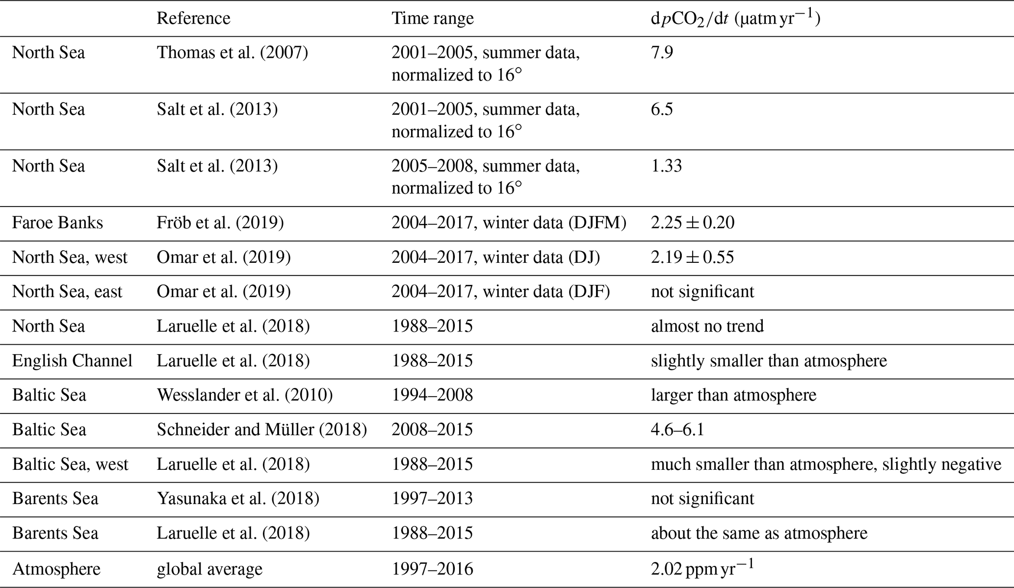
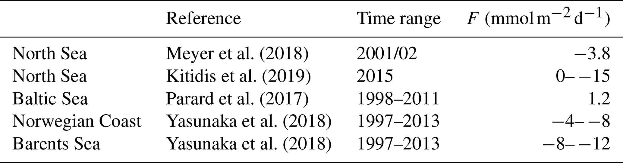
Table 2Overview of air–sea CO2 fluxes reported in the literature. Negative sign denotes flux from atmosphere to ocean.
Despite coastal seas covering 7 %–10 % of the world's oceans (Bourgeois et al., 2016), their contribution to the oceanic carbon sink is not yet fully constrained. Whether coastal seas are a net sink or source for atmospheric CO2 and how their role will change in a changing climate is still under debate (Bauer et al., 2013; Laruelle et al., 2010). Compared to the open ocean, longer time series and higher spatial and temporal resolution of the observations are needed in order to capture all relevant coastal processes. Small-scale circulation patterns governed by topographic features; thermal and haline stratification; or mixing through tidal cycles, upwelling or internal waves result in a need for more complex maps with a higher resolution (Bricheno et al., 2014; Lima and Wethey, 2012; Blanton, 1991). These physical drivers are not the only reasons for coastal seas being more complicated to understand. Generally, coastal regions are more productive than open-ocean regions due to better availability of nutrients (e.g., mixing at continental margins, river runoff). While deeper coastal regions are seasonally stratified, shallow regions are vertically mixed, allowing for exchange between the benthic and pelagic parts of the ecosystem (Griffiths et al., 2017; Wollast, 1998). Together with strong gradients of productivity this leads to spatial and temporal heterogeneity in surface CO2 content.
The different maps developed for describing the open-ocean surface pCO2 (CO2 partial pressure) dynamics and air–sea CO2 fluxes are not directly applicable in coastal regions. Many exclude data from continental shelves completely while all of them have too coarse a spatial resolution (typically between 1 and 5∘) to properly resolve coastal seas with their small-scale variability. A few studies have described coastal carbon dynamics, but most of them have strong regional or temporal limitations. Table 1 shows an overview of studies with estimated pCO2 trends over the northern European shelf, while Table 2 presents available flux estimates. Laruelle et al. (2017) used a neural network approach to produce a global pCO2 climatology for coastal seas, describing more distinct seasonal variability in the Northern Hemisphere than in the southern Pacific and Atlantic. A global climatology covering both open-ocean and coastal regions was recently constructed by combining this product with the open-ocean product of Landschützer et al. (2016, 2020). Laruelle et al. (2018) published trend estimates in regions with high data coverage based on winter data spanning up to 35 years. Their findings is that the pCO2 rise in coastal regions tends to lag the atmospheric rise in CO2. However, few studies attempted to constrain coastal air–sea fluxes before. Kitidis et al. (2019) estimated fluxes between 0 and −15 in the North Sea, depending on the season (more negative during summer than during winter) and the region (more negative fluxes in the northern North Sea compared to the south). For the Baltic Sea, Parard et al. (2016, 2017) used a neural network approach to produce surface ocean pCO2 maps from 1998 to 2011 and estimated an air–sea flux of 1.2 . Yasunaka et al. (2018) estimated a flux of 8–12 in the Barents Sea and along the Norwegian Coast using a self-organizing map technique. Most of the other available studies on the trends in coastal pCO2 are based on data from either summer or winter. Estimates based on summer-only data typically show large interannual variations (Thomas et al., 2007; Salt et al., 2013), which led to the conclusion that here the interannual variability masks the actual long-term trend. The approach to use winter-only data (Fröb et al., 2019; Omar et al., 2019), however, is based on the assumption that during this season the influence of biological processes is negligible and therefore winter data can be used to establish a baseline trend. However, also using winter-only data has its drawbacks. In particular the choice of which months to include can cause biases, and the optimal selection can differ from region to region.
In this study we present a new approach to develop monthly fCO2 (CO2 fugacity) maps based on already existing open-ocean pCO2 maps in four example regions: the North Sea, the Baltic Sea, the Norwegian Coast and the Barents Sea. A multi-linear regression (MLR) was used to fit driver data against fCO2 observations. Based on the resulting fCO2 maps and a salinity–alkalinity correlation we also produced monthly maps of coastal pH. The performance of the produced maps was evaluated, and the maps were then used to investigate trends in coastal fCO2 and pH in the entire region from 1998 to 2016. Finally, we used the fCO2 maps to determine the air–sea CO2 exchange and its temporal and spatial patterns.
2.1 Study area
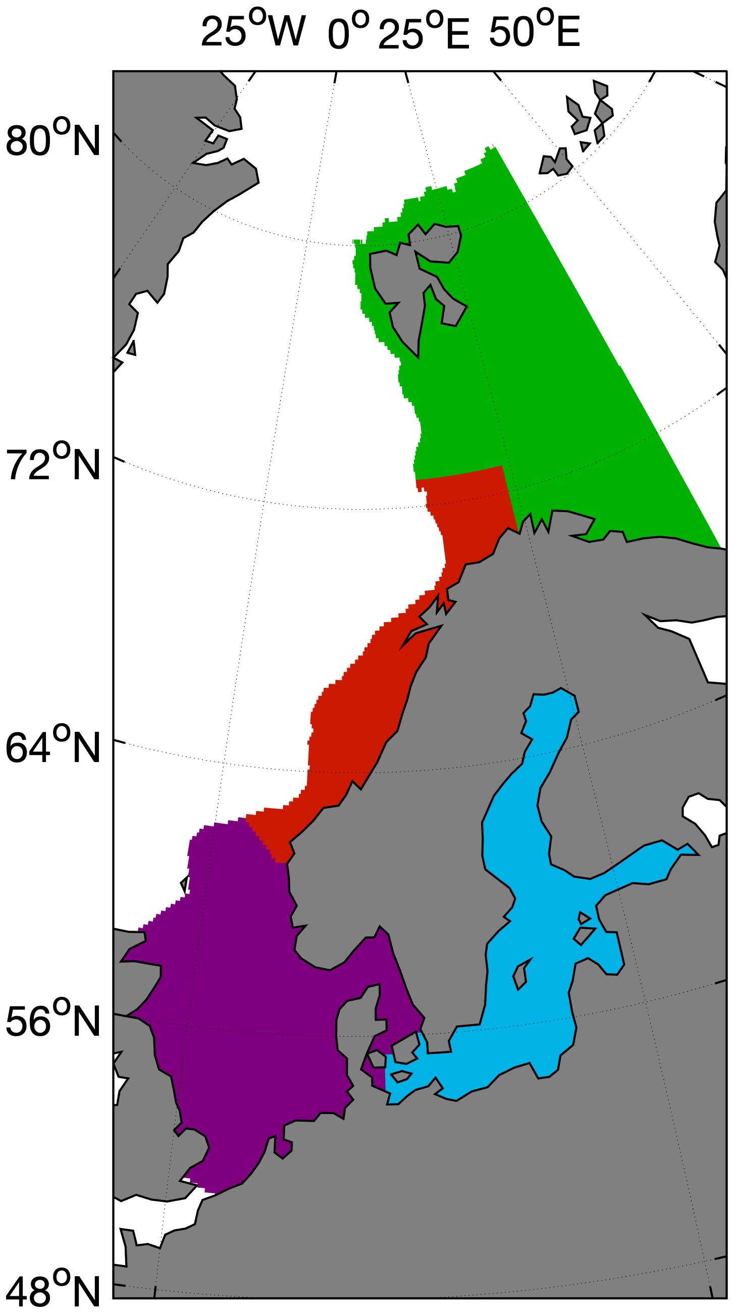
Figure 1The study area and the location of the four different regions: North Sea (purple), Norwegian Coast (red), Barents Sea (green) and Baltic Sea (blue).
This work focuses on the northern European continental shelf and marginal seas. As we want to show the performance of the MLR method we picked a number of regions with very different characteristics: the North Sea, the Baltic Sea, the Norwegian Coast and the western Barents Sea (Fig. 1). We decided to concentrate on these regions because (1) the data coverage in these regions is fairly high and (2) the authors have strong knowledge of the specific regions. This is important in order to properly evaluate the maps and to assess whether or not the output is realistic. The four regions were defined based on the COastal Segmentation and related CATchments (COSCAT) segmentation scheme (Laruelle et al., 2013). The threshold for defining a region as coastal sea was set to a depth limit of 500 m. By using this definition, we produce an overlap to the open-ocean maps, allowing our maps to be merged with the open-ocean maps. Please note that this study concentrates on the continental shelf area. The near-coastal zones (e.g., intertidal zones) are not included due to the limited availability of driver data in these regions.
2.2 Data handling
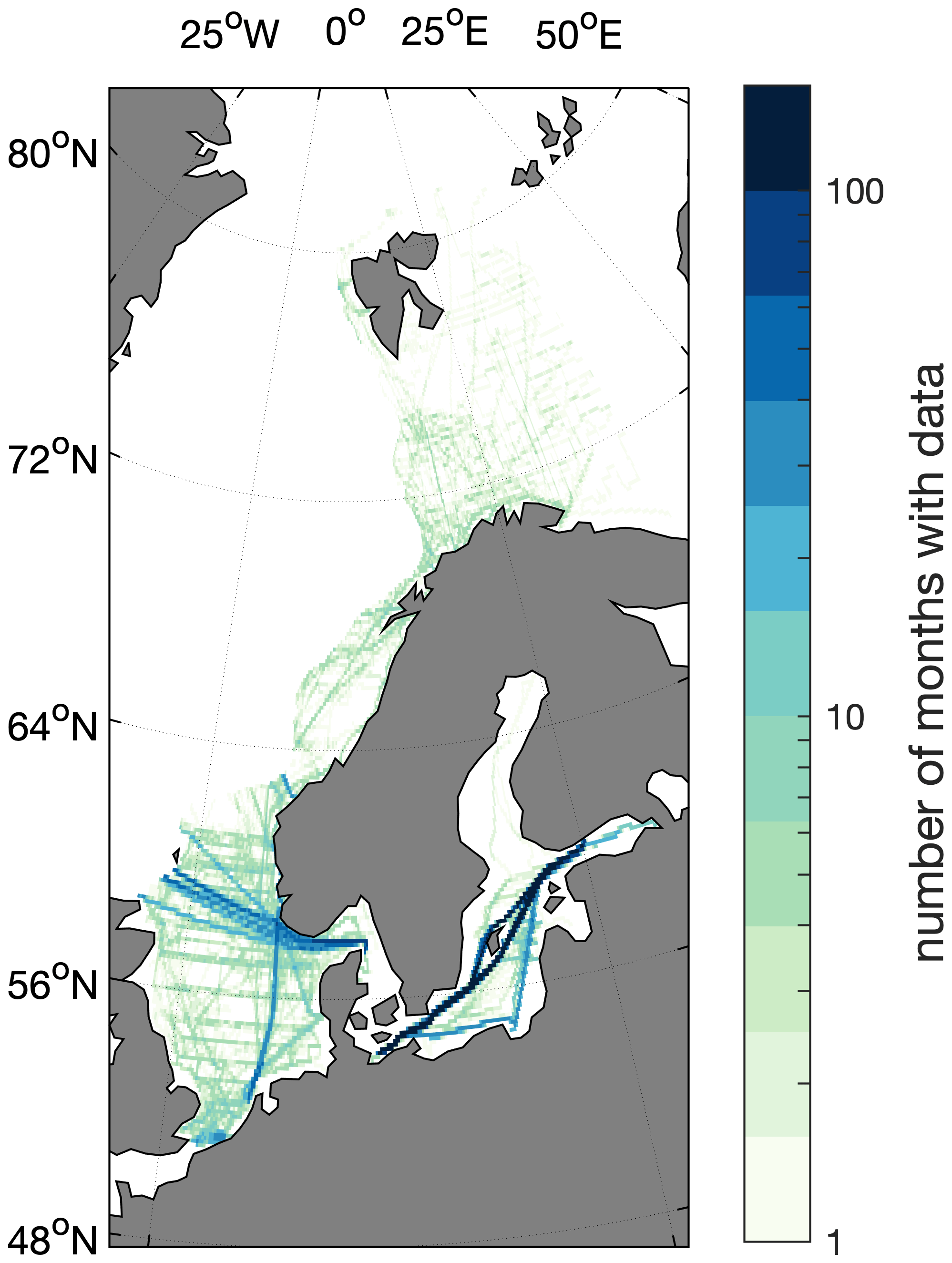
Figure 2The number of months with fCO2 data from SOCAT v5 in each grid box. The data cover a range of 20 years (240 months).
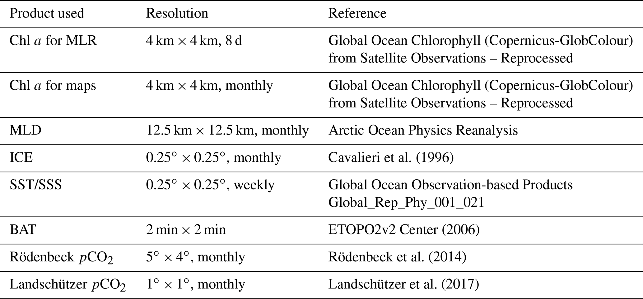
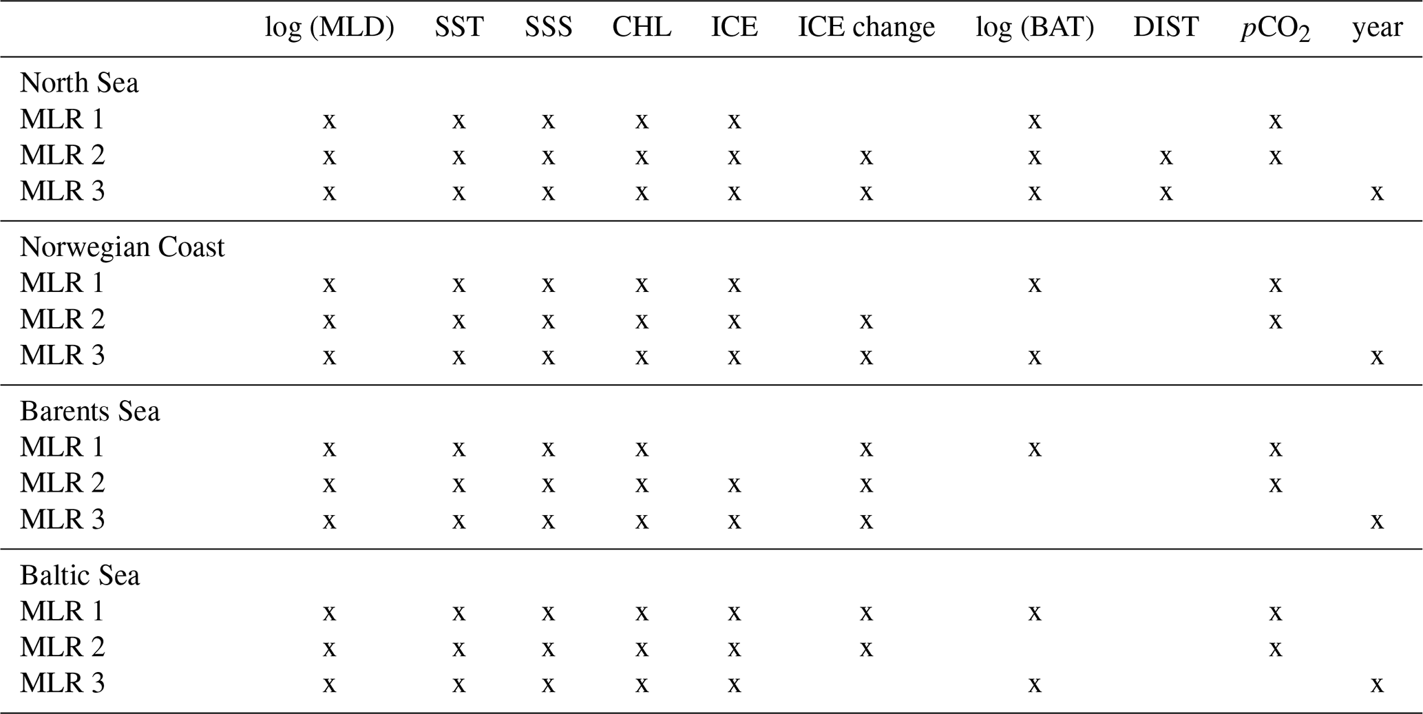
The CO2 data used in this study were extracted from Surface Ocean CO2 Atlas (SOCAT) version 5 (Bakker et al., 2016). Their coverage is shown in Fig. 2. A newer version of the SOCAT database (SOCATv2019) was used for validating the maps against independent data. An overview over the reanalysis products used as driver data is given in Table 3. We use as basic driver data sea surface temperature (SST), sea surface salinity (SSS), chlorophyll a concentration (Chl a), mixed layer depth (MLD), bathymetry (BAT), distance from shore (DIST), ice concentration (ICE) and the change in ice concentration from the month to month (prior to current). Chl a values during the dark winter season were set to 0. In addition to the reanalysis data, pCO2 values from the closest coastal grid cell of the open-ocean map were used as a driver in our MLR. We neglect the approximately 1 µatm difference between partial pressure (reported in the mapped products) and fugacity of CO2 (reported in SOCAT) as it is much smaller than the accuracy of the data extracted from SOCAT v5 (2 to 10 µatm) and the uncertainty associated with the open-ocean maps. The open-ocean pCO2 values were extracted from two different products (Rödenbeck et al., 2014, version oc_v1.5; and Landschützer et al., 2017, 2016, version 2016). Rödenbeck et al. (2014) is based on a data-driven diagnostic model of mixed layer ocean biogeochemistry fitted against surface pCO2 observations, while Landschützer et al. (2016) uses a two-step neural network (a feed-forward network coupled with self-organizing maps, FFN-SOM) trained with the pCO2 observations. Please note that the Rödenbeck open-ocean map contains data in coastal grid boxes, while the Landschützer open-ocean map is restricted to the open-ocean regions. The MLR models based on these two are called MLR 1 (based on the coastal pCO2 values from the Rödenbeck map) and MLR 2 (based on the nearest open-ocean pCO2 values of the Landschützer map), respectively. To determine the extent to which the regressions benefit from the information in the open-ocean maps, a third MLR, MLR 3, was determined. Here, we do not use any of the open-ocean maps as a driver, but to account for the annual rise in CO2, year is included in the set of driver data.
For preparing the input data for the MLR, observations closest to each SOCAT fCO2 data point in time and space were extracted from the 3-D fields with the driver data. This produces, for each of the driver data, a vector as long as the SOCAT fCO2 observations. After this, the fCO2 data as well as all extracted driver data were binned on a monthly 0.125∘ × 0.125∘ grid covering 1997 to 2016. These procedures ensure that the driver data have the same bias in space and time within each grid box as the fCO2 data. If a grid box for example only contains fCO2 observations from the first week of the month and the northwestern corner, we make sure that also the gridded driver data only contain values from the first week and the northwestern corner of the grid box, and not an average over the entire month and grid box. This is mostly important for the chlorophyll driver data, which are available at a very high resolution compared to the fCO2 maps produced in this work. These driver data were used for determining the MLRs.
For producing the final maps, a second set of the driver data was prepared, which is called field data in the following. Here the driver data were directly regridded to a monthly 0.125∘ × 0.125∘ grid, providing full spatial and temporal coverage and a homogeneous average in each grid box. The field data were used to produce the fCO2 maps based on the MLR equations.
2.3 Multi-linear regression
The multi-linear regression models were constructed by forward and backward stepwise regression using the driver data as predictor variables to model the fCO2 observations. In each step of this regression procedure, the model's tolerance to addition or exclusion of a variable is tested. This decision on whether to add or remove a term is based on the p value of the F statistic with or without the term in question. The entrance tolerance was set to 0.05 and the exit tolerance to 0.1. The model includes constant, linear, and quadratic terms as well as products of linear terms. Equation (1) gives the basic equation, with X1 … Xn being the driver data and a1 … ann the regression coefficients.
The pCO2 value of the respective open-ocean maps was used for MLR 1 and MLR 2, while year was always used as a driver variable in MLR 3. Inclusion of stationary drivers (such as month, latitude and longitude) in the MLR increased the performance of MLR 2 and MLR 3. However, these were still not better than MLR 1, and we therefore decided to limit this analysis to dynamic parameters. Using dynamic drivers only assures a dynamic description of the conditions in the field and gives us the possibility to reproduce changes caused by a regime shifts, for example the ongoing Atlantification of the Barents Sea (Oziel et al., 2017; Lind et al., 2018).
2.4 Validation
The three linear fits were compared to each other in each region by taking into account the R2 and the root mean square error (RMSE) of the fit, as well as the Nash–Sutcliffe method efficiency (ME) (Nondal et al., 2009). The method efficiency compares how well the model output (En) fits the observations (In) for every data point n to how well a simple monthly average () would fit the observations:
A method efficiency > 1 means that using just monthly averages of all data in the region would fit better to measured data than the respective model. Generally, a method efficiency > 0.8 is considered bad. Besides the statistics of the fit itself, the final maps were also compared to the gridded SOCAT v5 data, resulting in an average offset and standard deviation (SD). In order to compare the maps against data that were not used to produce the maps, we predicted the fCO2 for the years 2017 and 2018 (i.e., we applied the trained multi-linear model to driver data from 2017 and 2018) and compared these maps to fCO2 observations in SOCAT v2019, gridded on a monthly 0.125∘ × 0.125∘ grid. We also compare the maps directly with observations from repeated sampling locations in the North Sea and the Baltic Sea.
2.5 Ocean acidification
For calculating the pH, alkalinity (AT) was estimated in the North Sea, along the Norwegian Coast, and in the Barents Sea via a salinity–alkalinity correlation following Nondal et al. (2009). Alkalinity describes the capacity of the sea water to buffer changes in pH. As the concentration of most of the weak bases in seawater is strongly dependent on the salinity, alkalinity can in many regions be estimated from salinity. However, in regions with a high amount of organic bases in seawater, for example in strong blooms or at river mouths, deviations from the alkalinity–salinity relationship can occur. The carbonate system was calculated using the CO2SYS program (van Heuven et al., 2009) with carbonic acid dissociation constants of Mehrbach et al. (1973) as refitted by Dickson and Millero (1987), dissociation constants following Dickson (1990) and the boron–salinity relation following Uppström (1974). For the Baltic Sea, we did not calculate pH as the alkalinity–salinity relationship in this region is complex due to different AT–S relations in different sub-regions of the Baltic Sea and a non-negligible increase in AT over the last 25 years (Müller et al., 2016).
2.6 Calculation of trends
For calculating trends of fCO2 and ocean acidification, the data in every grid box were deseasonalized by subtracting the long-term averages of the respective months. Then a linear fit was applied to the deseasonalized time series. For illustrating the influence of interannual variability we calculated the trend for different time ranges. As a time range less than 10 years barely resulted in significant trends, we decided to limit the trend analysis to starting years 1998 through 2006 and ending years 2008 through 2016.
2.7 Flux calculation
The air–sea disequilibrium was calculated as the difference between our mapped fCO2 values and atmospheric fCO2 in each grid cell and time step. The atmospheric fCO2 was determined by converting the xCO2 from the NOAA marine boundary layer reference product from the NOAA GMD Carbon Cycle Group into fCO2 by using monthly SST and SSS data (Table 3) and monthly air pressure data from the NCEP-DOE Reanalysis 2 (Kanamitsu et al., 2002). We calculated the air–sea CO2 flux (F) according to Eq. (3), such that negative fluxes are into the ocean. The gas transfer coefficient k was determined using the quadratic wind speed (u) dependency of Wanninkhof (2014) (Eq. 4). The Schmidt number, Sc, was calculated according to Wanninkhof (2014) and the solubility coefficient for CO2, K0, following Weiss (1974).
In our calculations, we used 6-hourly winds of the NCEP-DOE Reanalysis 2 product. The coefficient aq in Eq. (4) is strongly dependent on the wind product used (Roobaert et al., 2018). We determined it to be aq = 0.16 cm h−1 for the 6-hourly NCEP 2 product following the recommendations of Naegler (2009) and by using the World Ocean Atlas sea surface temperatures (Locarnini et al., 2018). The barrier effect of sea ice on the flux was taken into account by relating the flux to the ice cover extent following Loose et al. (2009). As the gas exchange in areas that are considered 100 % ice covered from satellite images should not be completely neglected, we use a sea ice barrier effect for a 99 % sea ice cover in all grid cells where the sea ice coverage exceeded 99 %.
3.1 Maps of fCO2
Table 5Statistical evaluation of the MLR 1, MLR 2 and MLR 3 in comparison to the open-ocean maps of Rödenbeck et al. (2015) and Landschützer et al. (2017) for each region. The data for the open-ocean map of Landschützer et al. (2017) are in parentheses since this is based on an extrapolation of the nearest open-ocean grid cell towards the coast. The number of grid cells containing data is given behind the region abbreviations.

The skill assessment metrics for MLR 1, MLR 2 and MLR 3 are presented in Table 5. It shows the R2 and RMSE of the fit, the ME, and the average offset and SD to the gridded SOCAT data. The coefficients for MLR 1, MLR 2 and MLR 3 are provided in the Supplement. The MLRs substantially improve the predictions of the open-ocean maps in all studied regions, showing a better average offset and SD to SOCAT v5 and ME than the coarser-resolution open-ocean maps (for example the Rödenbeck map: North Sea, 0 ± 95 µatm; Norwegian Coast, 2 ± 17 µatm; Barents Sea, 22 ± 40 µatm; Baltic Sea, 4 ± 48 µatm; MLR1: North Sea, 0 ± 26 µatm; Norwegian Coast, 0 ± 16 µatm; Barents Sea, 0 ± 19 µatm; Baltic Sea, 2 ± 42 µatm). In all regions MLR 1 has the best model efficiency, the highest R2 and the smallest RMSE of the fit, while these statistics are worse for MLR 2 and MLR 3. This can be explained by the fact that the Rödenbeck map contains information about the continental shelf and the Barents Sea, while for MLR 2 the closest open-ocean grid cell of Landschützer et al. (2017) was used. The fact that MLR 3 showed the weakest performance shows the value of using information from the open-ocean maps in the regression.
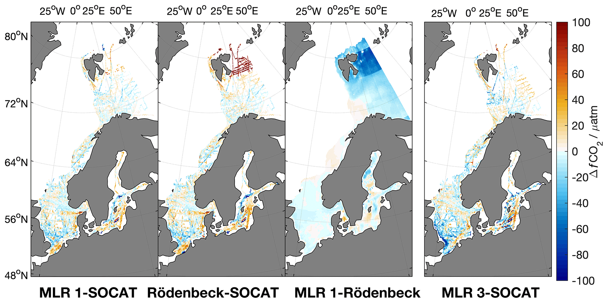
Figure 3Average regional differences between MLR 1 and gridded SOCAT v5 data, the Rödenbeck map and gridded SOCAT v5 data, MLR 1 and the Rödenbeck map, and MLR 3 and the gridded SOCAT v5 data (from left to right).
Figure 3 shows, from left to right, the spatial distribution of the average difference between the predicted fCO2 by MLR 1 and the gridded SOCAT v5 data, the Rödenbeck map and the gridded SOCAT v5 data, the difference between MLR 1 and the Rödenbeck map, and, for comparison, the difference between MLR 3 and the SOCAT v5 data. In the North Sea, MLR 1 seems to slightly overestimate the fCO2 in the constantly mixed region at the entrance of the English Channel and the area off the Danish North Sea coast. In the Baltic, MLR 1 generally describes the spatial variability in fCO2 well. However, in the Gulf of Finland it usually predicts fCO2 values that are too low during May/June while it slightly underestimates events of very high fCO2 in December/January. Regardless, the spatial biases vs. SOCAT are clearly smaller for MLR 1 than for the original Rödenbeck map. Further, as the predictions of MLR 2 and 3 are clearly inferior to those of MLR 1 (Table 5 and Fig. 3, MLR 3 only), we will use MLR 1 results for the further analyses. An extended validation of the MLR 1 maps can be found in the discussion section.
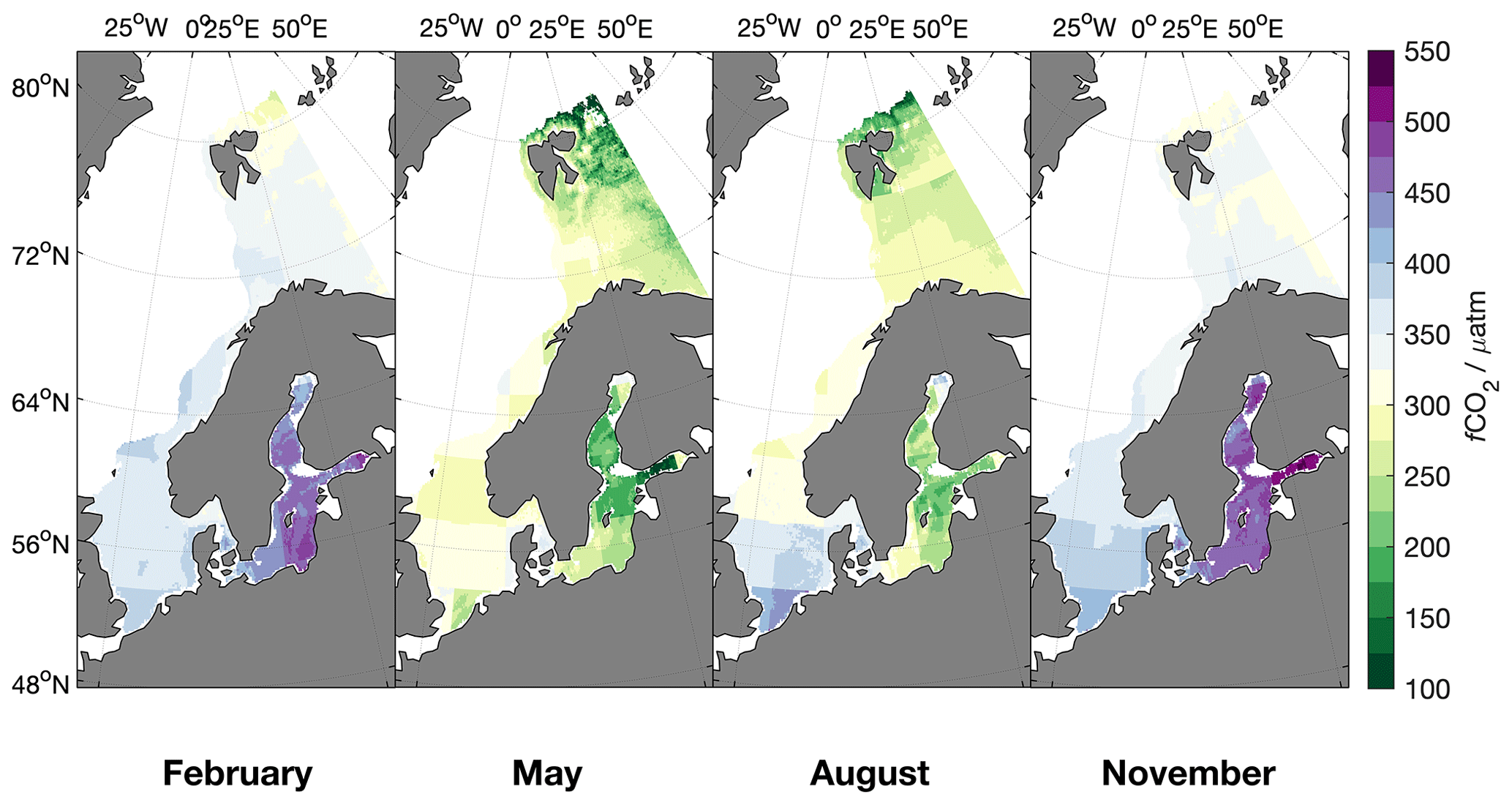
Figure 4The average fCO2 of MLR 1 (1998–2016) for 1 example month in each season (February, May, August and November).
Figure 4 shows the monthly averages of fCO2 produced by MLR 1 for February, May, August and November. In all regions, the highest fCO2 values occur in the winter, while the lowest fCO2 values occur in summer. The largest seasonal cycle could be observed in the Baltic Sea, where fCO2 reached well below 200 µatm in midsummer and over 500 µatm during the winter.
We notice that the gradients that exist between the grid cells in the Rödenbeck map are still visible in our maps in some regions, for example the sharp gradient in the southern North Sea in February or the east–west and north–south gradients in the entire North Sea in August. Such gradients are also evident in directly mapped pCO2 data (Kitidis et al., 2019); however, here they are strongly meridional and latitudinal in their extent. As such, while these gradients do reflect actual features of the fCO2 distribution in the North Sea, their specific shape here is also a consequence of the influence of the Rödenbeck maps on our estimates – from the use of these maps as a driver in the MLR and their importance in improving the statistical performance vs. the MLR that did not use these values as a driver (MLR 1 vs. MLR 3, Table 5). Also, they do reflect the uncertainty of – and our level of confidence in – the estimated pCO2 values, being approximately similar to or slightly larger than the RMSE of MLR 1 (Table 5). Any smoothing would be completely artificial and, while being more visually pleasing, would not better reflect the truth in any meaningfully quantifiable extent. We have therefore chosen to leave them untouched. These gradients are therefore also visible in subsequent pH and trend maps.
3.2 Maps of pH
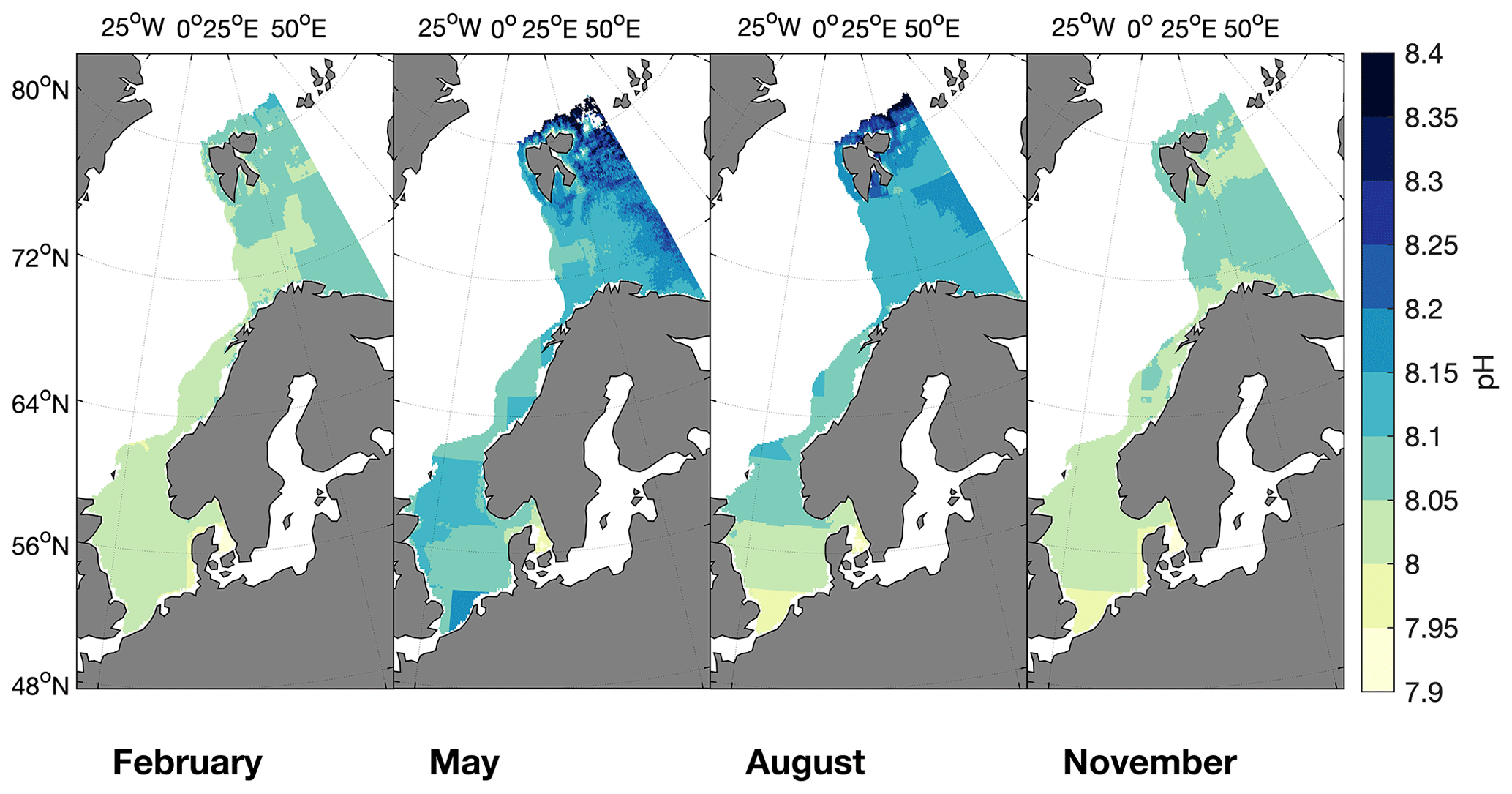
Figure 5The average pH based on MLR 1 (1998–2016) for 1 example month in each season (February, May, August and November).
The monthly average of pH calculated from MLR 1 fCO2 ranges from about 8 during winter to 8.15 during summer in the North Sea and at the Norwegian Coast (Fig. 5). Towards the Barents Sea the pH maximum during summer increases to 8.2. The pH of 8.00–8.15 in regions with a large influence from the Atlantic, such as the northern North Sea and the Norwegian Coast, is in good agreement with the range of pH determined for the open North Atlantic (Lauvset and Gruber, 2014; Lauvset et al., 2015). In the North Sea, the pH is in the same range as reported in Salt et al. (2013), and it also shows the same distribution in August/September, with higher pH in the northern North Sea and lower pH in the southern part.
4.1 Performance of the pCO2 maps
The performance of the MLR and the maps is evaluated in different ways: (1) using the R2 and the RMSE of the fit; (2) using the average deviation and its SD, as well as the ME between the produced fCO2 maps and the gridded observations as a regional average; (3) showing the median deviation between the MLR and the gridded observations on a monthly level; and (4) by comparing the data from the fCO2 maps to observations from two time series stations. (2)–(4) will be shown for the time period covered by the driver data (1998–2016) and for the prediction of the fCO2 values for 2017 and 2018. These predicted values are compared with data from the newest SOCAT release (SOCATv2019) and provide a comparison with an independent dataset. Please note that the comparability of the model performance between the different regions is limited. All statistical parameters used are influenced by characteristics that can vary substantially between the different regions, such as range of the data, their variability or the amount of grid cells with data. For example, in a diverse region with many measurements the amount of variability captured by these measurements is most likely larger and thus will lead to a weaker correlation.
Generally, the uncertainty of MLR 1 is in the same range as in other studies (Laruelle et al., 2017; Yasunaka et al., 2018) mapping coastal fCO2 dynamics: 25 µatm in the North Sea, 16 µatm along the Norwegian Coast, 12 µatm in the Barents Sea and 39 µatm in the Baltic Sea (based on the RMSE in Table 5). In the Baltic Sea, which has a large variability in itself, Parard et al. (2016) obtained lower SDs through dividing the area in smaller sub-regions.
One clear drawback of the here presented MLR 1 is the clearly visible grid pattern of the open-ocean pCO2 product that was used as input data with its grid size of 5∘ × 4∘, mentioned in Sect. 3.1. There are two ways how one could get rid of this artifact in a future release. A finer resolution of the open-ocean maps used will lead to a better representation of the actual gradients in our mapped product. Rödenbeck et al. just released a newer, finer resolution of their open-ocean product (2.5∘ × 2∘) that we intend to use in a future version of this data product. However, this will not be sufficient to eradicate the artifact completely. Another approach, running the MLR without an open-ocean pCO2 product, can provide a coastal pCO2 product without this artifact. While in principle it is preferential to have coastal maps that are independent of the open-ocean products, MLR 3, which is running without open-ocean pCO2 as a driver, clearly did not reach the same accuracy as MLR 1 (Table 5). New and better input fields or a different regression method could help improve the independent coastal maps in the future. Another impact that the open-ocean pCO2 product of Rödenbeck et al. can have on MLR 1 is the potential introduction of patterns from regions further away as the spatial correlations used in producing the Rödenbeck et al. pCO2 just ignore land barriers. However, the influence of these spatial correlations is relatively small in regions with a high data density (as the European shelf) and the multi-linear regression used to produce MLR 1 corrects for this.
The seasonal differences between MLR 1-determined values and the SOCAT v5 data for each region are shown in Fig. 6. This comparison shows a very good agreement. For MLR 1, the seasonal variations of the median bias are small in the North Sea, along the Norwegian Coast and in the Baltic Sea. In the Barents Sea, however, the bias varies seasonally. Here, MLR 1 slightly underestimates the fCO2 in winter and early spring, while it overestimates the fCO2 in summer. In all other regions, the median seasonal bias is smaller than the uncertainty of the maps. The larger seasonal bias in the Barents Sea is most likely caused by the larger seasonal bias in the number of available observations. There are no data available in October, December and January.
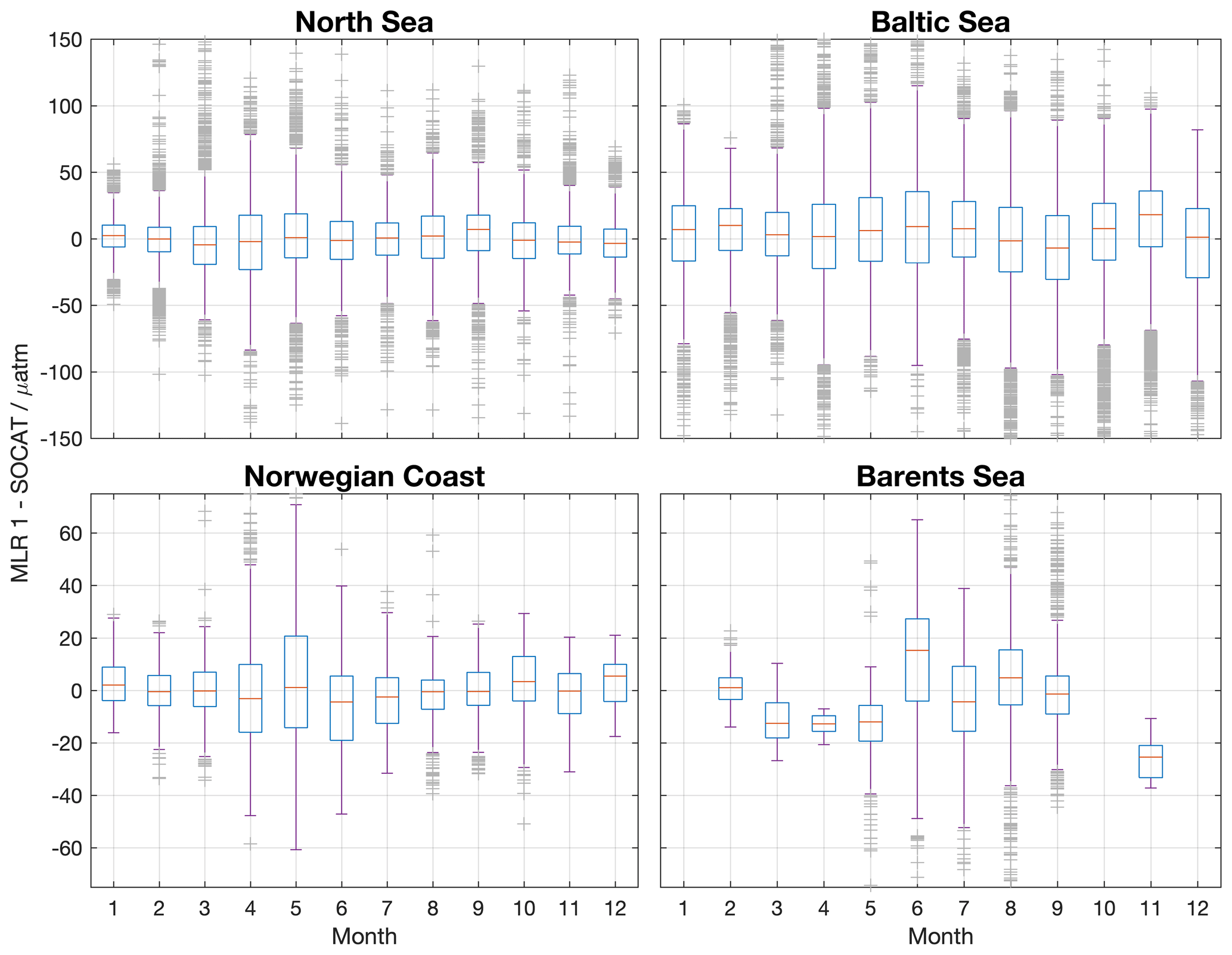
Figure 6Boxplots showing the median deviation of MLR 1 from the gridded SOCAT 5 data for each region (red line). The boxes show the upper and lower 75th percentiles. Ninety-nine percent of the data lie within the range of the purple whiskers. Extremes are shown as gray crosses.

Figure 7Boxplots showing the median deviation between MLR 1 (based on observations until 2016) and measured fCO2 values in 2017 and 2018. The boxes show the upper and lower 75th percentiles. Ninety-nine percent of the data lie within the range of the purple whiskers. Extremes are shown as gray crosses. The numbers of grid cells with data available were 5047 for the North Sea, 1543 for the Norwegian Coast, 2312 for the Barents Sea and 5414 for the Baltic Sea.
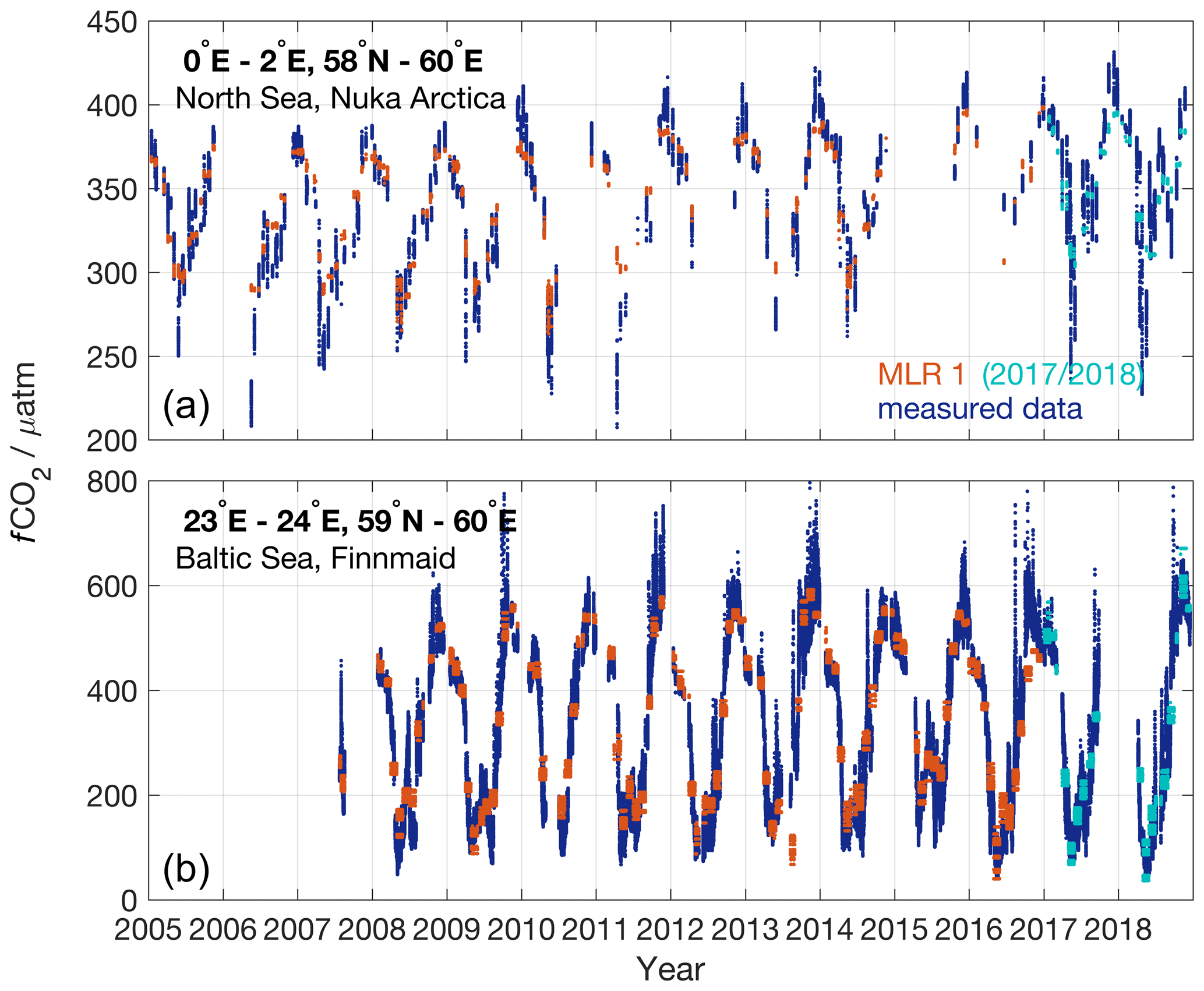
Figure 8Time series of ship-of-opportunity (SOOP) data from Nuka Arctica (a, blue) and Finnmaid (b, blue) compared with MLR 1 at the same location (red). In light blue the predictive MLR output for the years 2017 and 2018 is shown.
When comparing all observations from the years 2017 and 2018 to the predictions by the MLR 1, we find a good agreement in the North Sea (2±20 µatm) and no seasonal bias (Fig. 7). In the other regions, the agreement is somewhat reduced compared to the years 1997–2016 (−9 ± 39 µatm (Norwegian Coast), −5 ± 29 µatm (Barents Sea) and 28 ± 58 µatm (Baltic Sea)). In these regions we also observe a seasonal bias in the years 2017 and 2018. At least for the Baltic Sea this could be a result of the extraordinary warm and dry summer in 2018 that led to very low fCO2 values (see Fig. 8 and the data in SOCAT, Bakker et al., 2016). Please note that for this comparison the MLR was extrapolated in time. Only observations until December 2016 were used to produce the MLR. Therefore accuracy of the maps itself is reduced.
In a second test to investigate to which extent MLR 1 can reproduce observations we compared the MLR output with time series data from two voluntary observing ship lines in two very different regions with a good data coverage: M/V Nuka Arctica in the northern North Sea (0–2∘ E, 58–60∘ N) and M/V Finnmaid in the Baltic Sea (23–24∘ E, 59–60∘ N) (Fig. 8). The agreement between the MLR 1 and the observations is very good. MLR 1 reproduces the general seasonality and some of the interannual variability, also in the years 2017 and 2018, the observations of which were not used in the regression.
When performing interpolation exercises it is always important to be aware of the fact that the resulting maps might come with biases and do not represent all regions equally well. While the here presented maps give a good general overview about the surface ocean fCO2 variability in regions with a relatively large amount of data, the reliability, however, is limited in regions where the data coverage is more scarce. This is especially the case when the region with scarce data coverage is showing different characteristics in, for example, temperature and salinity, compared to the rest of the region. One such example is the Gulf of Bothnia in the Baltic Sea region where almost all data used to derive the MLR is from south of 60∘ N, i.e., not in the Gulf of Bothnia but in the Baltic Proper and western Baltic Sea (see Fig. 2). The MLR method can also lead to unrealistic extreme values and even negative fCO2. Some such values occur in the northeastern Barents Sea as well as in parts of the Baltic Sea (about 0.01 % of the grid cells in each region). As pH cannot be calculated for negative fCO2, we excluded all negative fCO2 values for the calculation of pH. Excluding the negative values resulted in a change in the average fCO2 of 0.05 µatm (Baltic Sea) and 0.3 µatm (Barents Sea) so they are of negligible importance for the flux estimates. While the negative values are easy to spot and discard, there are most likely other unrealistically low values in spring and summer in the very north and northeastern Barents Sea as well as some parts of the Baltic Sea. However, there are no data available in SOCAT v5 or available elsewhere to validate this.
All regions with questionable fCO2 are also questionable in their pH data. There is a number of very high pH regions in the Barents Sea (Fig. 5) that are associated with also very low fCO2 (Fig. 4) that might not be realistic. In addition, estimated pH values in low-salinity regions where the actual alkalinity–salinity deviates strongly from the Nondal et al. (2009) one used here (e.g., river mouths in the southern North Sea or the Skagerrak) should be interpreted with caution.
4.2 Trends in fCO2 and pH
Trends in surface ocean fCO2 in coastal regions are often difficult to assess because of the scarcity of data relative to the highly dynamical character of these regimes and their large interannual variability. For example, the start of the productive season can range from February to April even within a small area, such that even restricting the analysis to specific seasons (e.g., winter) can be challenging. Also, due to a lack of data, especially winter data, most observational studies are based on summer data. Further, the fact that these measurements typically do not take place every year adds even more uncertainty to the estimated trend, as interannual variability can mask the trend signal.
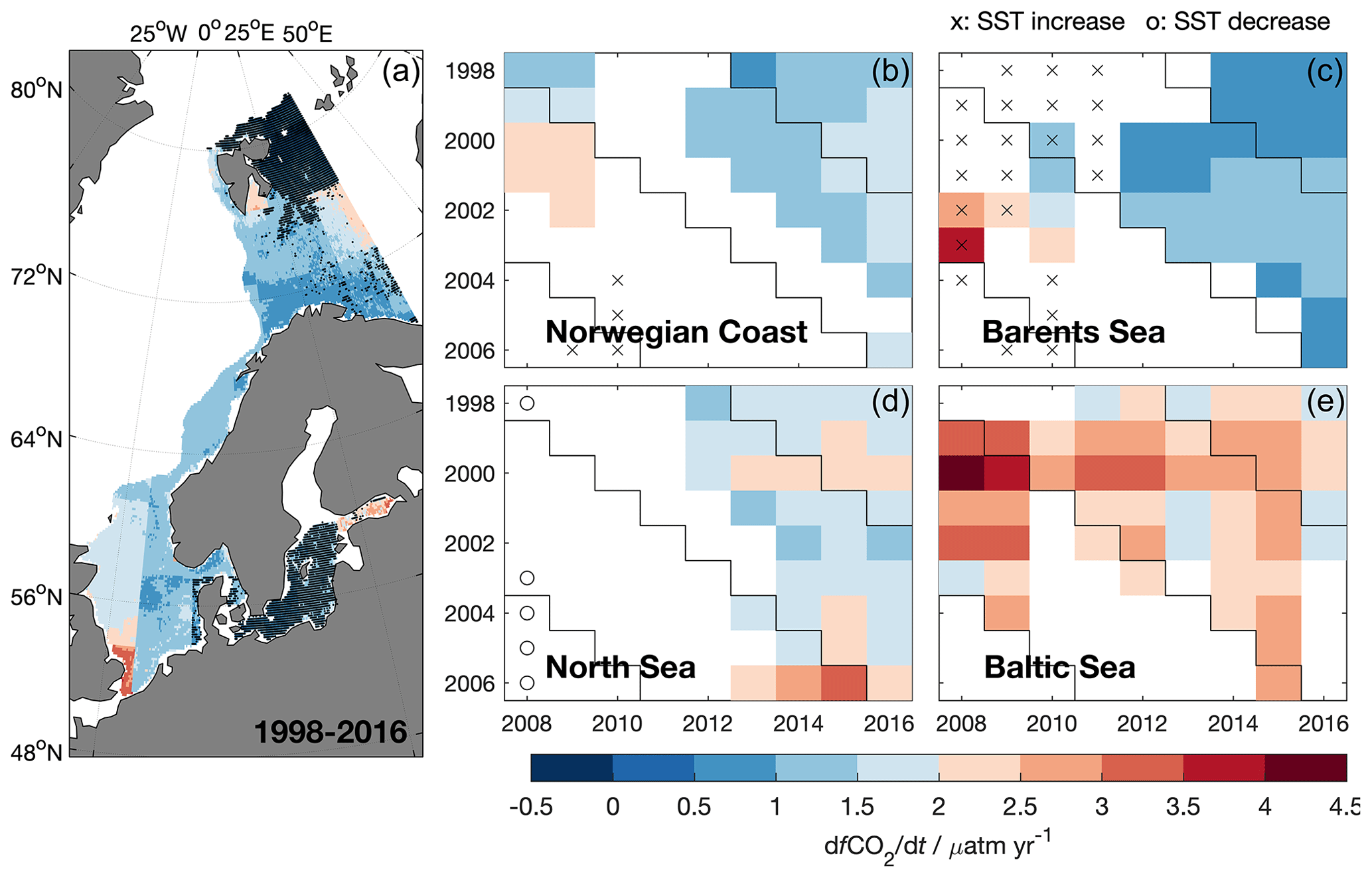
Figure 9The trend in surface ocean fCO2 estimated from deseasonalized fCO2. Panel (a) shows the spatial distribution of the trend over the time period from 1998 to 2016. Grid boxes without a significant trend are denoted with a black dot. Panels (b)–(e) show the trends in different time periods in four regions, from the various years on the y axis to the various years on the x axis. Non-significant trends were left blank. Significant trends in sea surface temperature are indicated with crosses/circles. The color bar is centered on the approximate annual fCO2 rise in the atmosphere (2 µatm yr−1).
The monthly maps of fCO2 from 1998 to 2016 enable us now to estimate the trend in surface ocean fCO2 for the entire region, equally distributed over the seasons (Fig. 9, left). All trends were computed from deseasonalized data. The interannual variability of the trend estimates in each region is shown in the panels on the right hand side in Fig. 9. We exclude the northern Baltic Sea from the trend map because we do not expect to have a robust trend estimate in that region as there are only very few data from that region in the regression. Based on the linear regression the significant trends in fCO2 have an average uncertainty of 0.5 µatm yr−1 (North Sea), 0.4 µatm yr−1 (Norwegian Coast), 0.4 µatm yr−1 (Barents Sea) and 0.7 µatm yr−1 (Baltic Sea), while the shorter time periods shown have a higher uncertainty; no time periods longer than 1998–2016 (for which the given uncertainties of the trend apply) are shown. For pH trends, the average uncertainties of the regressions over 1998–2016 are 5 × 10⁻⁴ (North Sea) and 7 × 10⁻⁴ (Norwegian Coast and Barents Sea).
In most of the regions addressed in this study, the trend in the surface ocean is lower than the trend in atmospheric xCO2 (global average 2.02 ppm yr−1 (Cooperative Global Atmospheric Data Integration Project, 2015)). Trends exceeding the atmospheric values in the period from 1998 to 2016 can only be observed at the entrance of the English Channel, in Storfjorden/Svalbard and the Gulf of Finland (2.5–3 µatm yr−1). It has to be noted that there was almost no measured fCO2 as MLR input from Storfjorden. Therefore, these trends are highly uncertain. The trend in the western North Sea is only slightly lower than the trend in the atmosphere (1.5–2 µatm yr−1), while the trends in the eastern North Sea, along the Norwegian Coast and in the Barents Sea are lower (0.5–1.5 µatm yr−1). In the North Sea this is consistent with a recent study of Omar et al. (2019), which is directly based on observations. These low trends will result in an increase in the strength of the ocean carbon sink with time.
Table 6fCO2 trend calculated from gridded, deseasonalized SOCAT v5 observations.
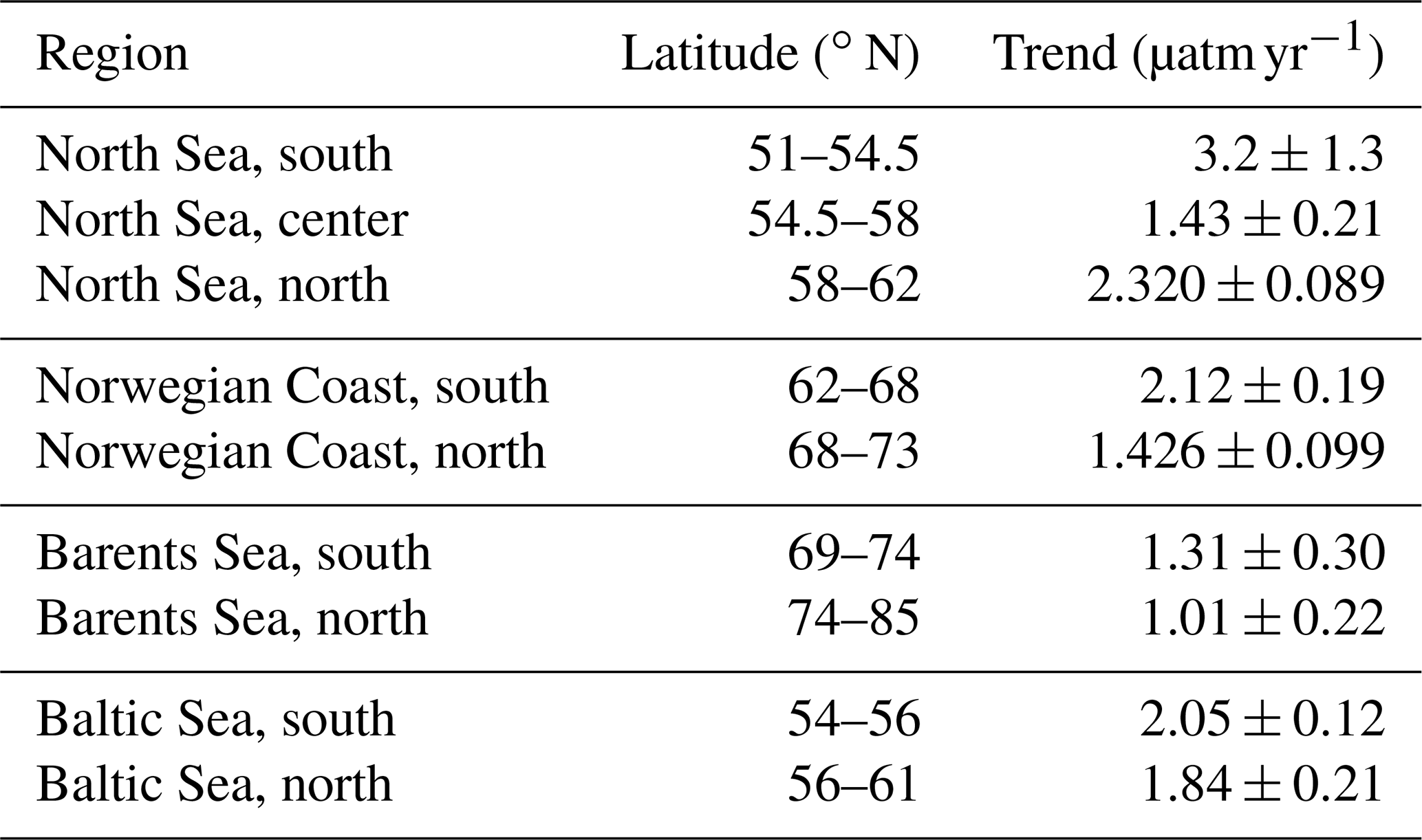
Generally, only few regressions over time ranges of less than 10 years turned out to be significant. This is an important finding when comparing the trends determined from our maps with the trends reported in literature, many of which were covering periods shorter than 10 years (Table 1). In order to compare the general patterns of fCO2 trends determined from our maps with those directly determined from observations over a similar time range, we estimated the fCO2 trends also from the SOCAT v5 observations that were used to produce the MLR (Table 6). We gridded and deseasonalized the SOCAT v5 data and divided the entire region into nine subregions. A figure showing the fits and the data coverage can be found in Appendix A. These observation-based trends show similar general patterns as those based on our maps (Fig. 9, 1998–2016): (1) largest trends in the southern North Sea, (2) decreasing towards the north with trends around the atmospheric trend in the northern North Sea and trends around 1 µatm yr−1 in the Barents Sea, and (3) close to atmospheric trends in the Baltic Sea.
The observation that some subareas (the Baltic Sea or along the shore of the western North Sea) did not show a significant trend can be explained by the fact that coastal sea systems, especially enclosed areas such as the Baltic Sea, experience a high anthropogenic pressure. Anthropogenic impacts other than rising atmospheric CO2 concentrations influence the ocean carbon system; for example the nutrient load of rivers can affect coastal ecosystems and primary production through eutrophication. This will result in lower fCO2 in summer and higher fCO2 in winter (Borges and Gypens, 2010; Cai et al., 2011). Another important process that influences the carbon system in the Baltic Sea is inflow events from the North Sea. In between such events, CO2 accumulates in deeper water layers, causing an increasing gradient of dissolved inorganic carbon (DIC) across the halocline. Whenever deep winter mixing occurs, this will then lead to a large increase in surface fCO2 because of the input of DIC-rich waters from below. Another reason is the observed change in alkalinity with time. This affects the fCO2 though changes in the buffer capacity of the inorganic carbon system (Müller et al., 2016).

Figure 10(a) The long-term trend (1998–2016) in surface ocean fCO2 each month. (b) The average seasonality in fCO2 for the periods 1998–2007 (green) and 2007–2016 (purple) in the northeastern North Sea (58–60∘ N, 3–8∘ E), normalized to December. The SD for each month is shown as the shaded area.
In most other regions, the sea surface fCO2 trends were typically smaller than the rise in the atmospheric CO2 concentration. A possible explanation is an earlier onset of the spring bloom. For example, in the North Sea a significant drawdown in fCO2 has been observed as early as February in some years, but there is also a large variability (Omar et al., 2019). The bloom timing and onset in the North Sea after the 1990s have been shown to be mainly triggered by the spring–neap tidal cycle and the air temperature (Sharples et al., 2006). The bloom timing and onset were found to be significantly earlier in the 2010s compared to the previous decades (Desmit et al., 2020). Even if the trend in winter fCO2 was following the atmospheric xCO2 increase, such a change in bloom timing and onset would lead to a trend lower than in the atmosphere when averaging over the entire year. Figure 10a shows the annual trends in fCO2 in each month in the four regions considered. Particularly in the North Sea and Baltic Sea, very low fCO2 trends are observed in February–May, suggesting that changing timing of the spring bloom might be important here. Investigating the seasonal fCO2 in more detail (Fig. 10b) revealed an earlier and deeper fCO2 drawdown in the second decade of our analysis (2007–2016) than in the first (1998–2007) in the northeastern North Sea (58–60∘ N, 3–8∘ E). This strongly suggest that an earlier and stronger spring bloom is lowering the annual fCO2 growth rates in this region, which is among the ones with the smallest fCO2 trends in the North Sea (about 1 µatm yr−1, Fig. 9). In the other regions, no such changes could be established with confidence. Future investigations should aim at generating fCO2 maps with higher temporal resolution, as changes in the timing of the spring bloom might be a matter of days or weeks, which would not be fully resolved by the monthly maps presented here.
When looking at the interannual variability, it becomes obvious that the trend in the North Sea is slightly smaller than the atmospheric CO2 trend. In contrast, the Norwegian Coast and the Barents Sea experience a robust trend much lower than the atmospheric trend (Norwegian Coast: 1–1.5 µatm yr−1; Barents Sea: around 1 µatm yr−1). Here we can also see a stable pattern of warming over timescales of 10 to 15 years. The warming in itself would result in an increase in fCO2 with time, in addition to the atmospheric forcing. As we are observing a trend smaller than the atmospheric trend, temperature effects cannot be the driver here. The lower trend stems most likely from an earlier onset of spring bloom. It has been shown that the Atlantification and the reduced ice coverage of the Barents Sea lead to a longer productive season, and this will result in more months with strong undersaturation in CO2 (Oziel et al., 2017). In the Baltic Sea the patterns are different. Here the variability is much larger, while most of the time periods show a trend larger than the atmospheric trend (3–3.5 µatm yr−1). Although slightly smaller our results broadly agree with trend estimates based on measurements of 4.6–6.1 µatm yr−1 over 2008–2015 (Schneider and Müller, 2018). Finally, it also needs to be noted that the uncertainty of the fCO2 maps was highest in the Baltic Sea. This makes it also more difficult, if not impossible, to properly detect these small differences in the trends.
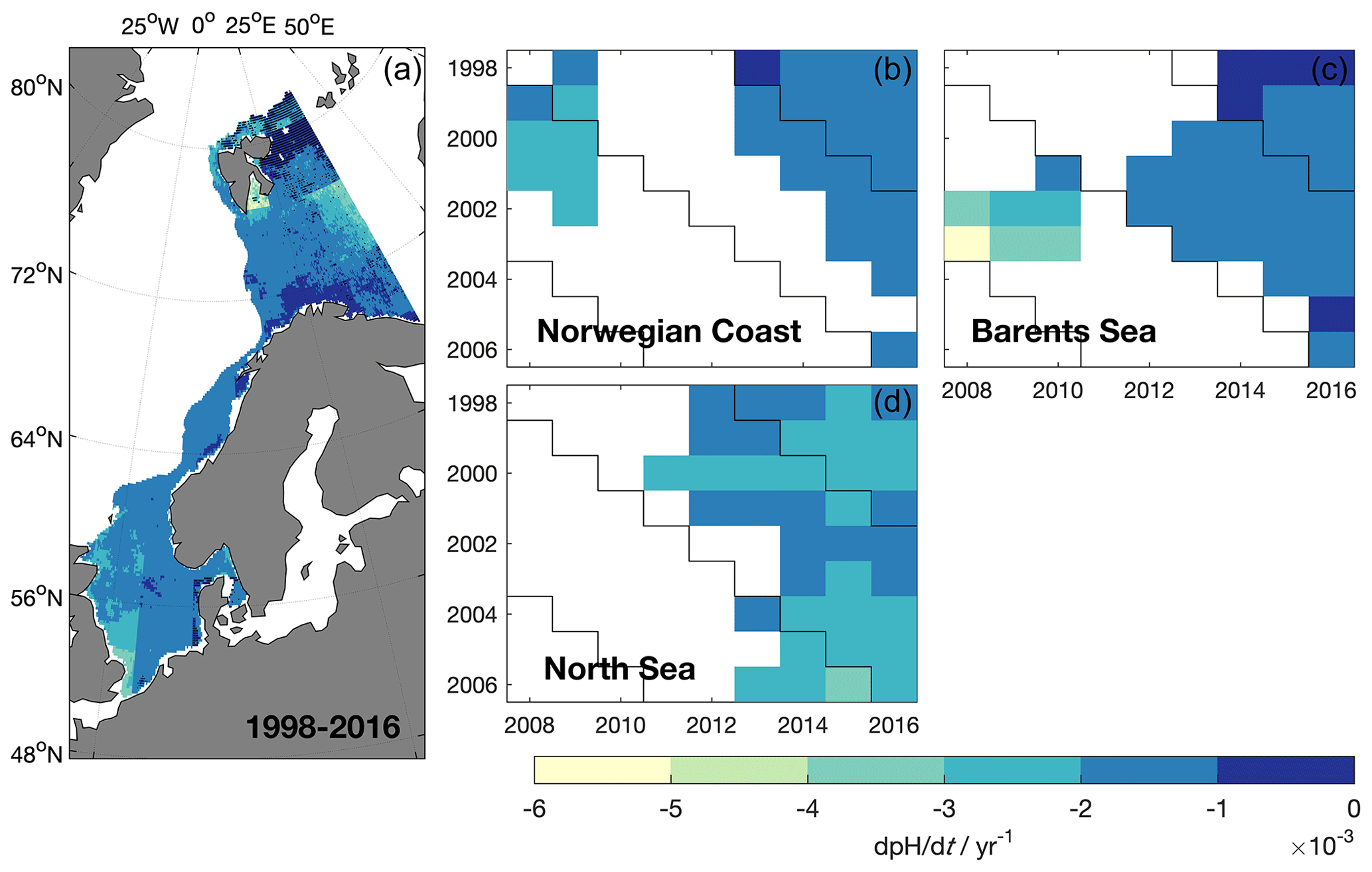
Figure 11The trend in surface ocean pH estimated from deseasonalized pH. (a) The spatial distribution of the trend over the time period from 1998 to 2016 is shown. Grid boxes without a significant trend are denoted with a black dot. Panels (b)–(e) show the trends in different time periods in three regions, from the various years on the y axis to the various years on the x axis. Non-significant trends were left blank.
For pH, the trend in most regions is around −0.002 yr−1 (Fig. 11). As expected, regions with the strongest trend in fCO2 also show the highest trend in pH, such as the southern North Sea. The trend in the northern North Sea and along the Norwegian Coast is in good agreement with the pH trends found in studies focusing on the open Atlantic Ocean (−0.0022 yr−1, Lauvset and Gruber, 2014) and the North Atlantic and Nordic Seas (−0.002 yr−1, Lauvset et al., 2015).
4.3 CO2 disequilibrium and flux
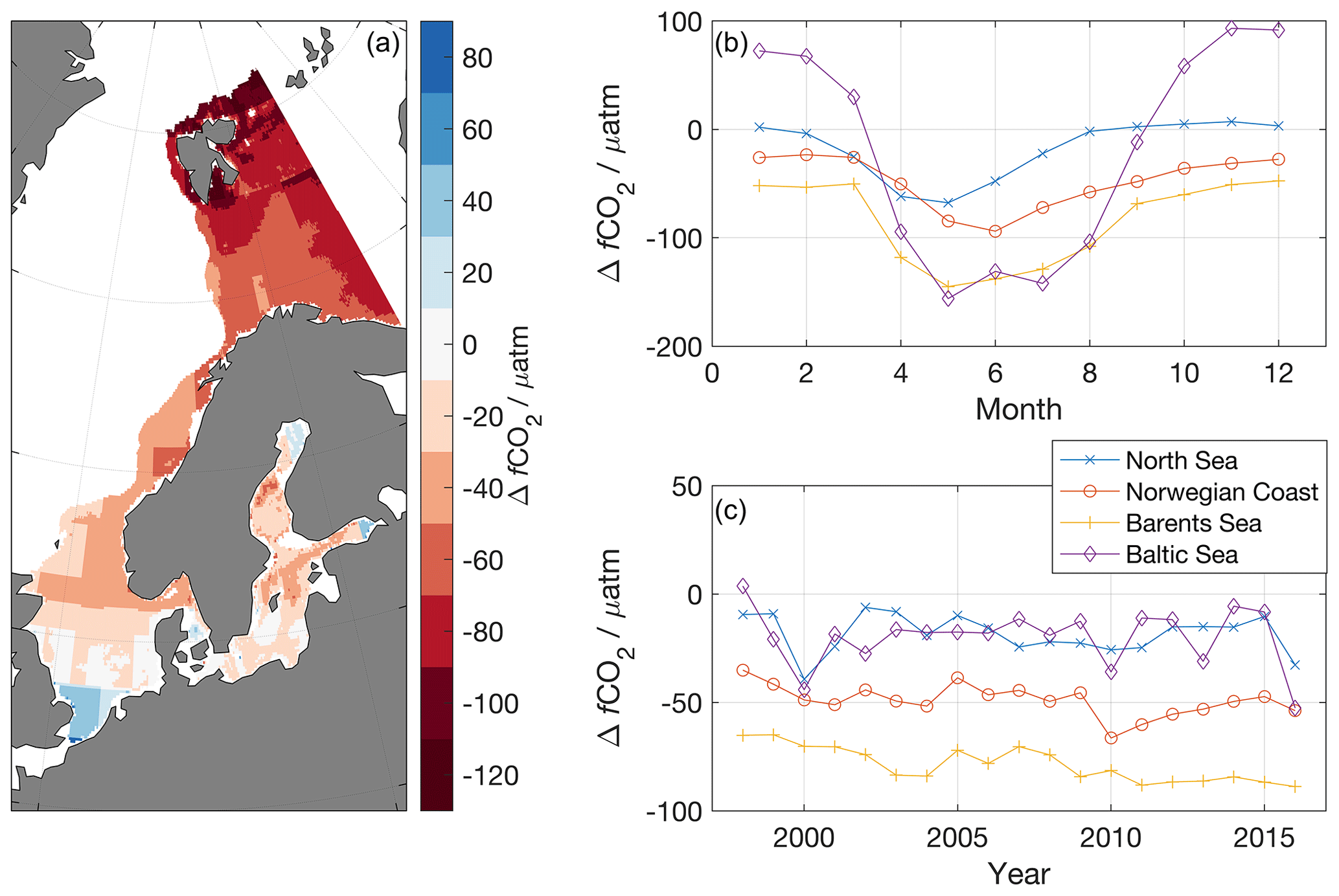
Figure 12The average air–sea CO2 disequilibrium over the period 1998–2016 (a, red colors indicate average undersaturation, while blue colors indicate average oversaturation). For every region average disequilibria are shown as seasonal averages (b) and time series of annual disequilibria (c). Blue line: North Sea; red line: Norwegian Coast; yellow line: Barents Sea; purple line: Baltic Sea
The average air–sea CO2 disequilibrium (ΔfCO2 = fCO2,sea − fCO2,atm) is shown in Fig. 12. The only region showing an average supersaturation is the southern North Sea. Towards the north, the surface ocean becomes more and more undersaturated, with the lowest values in the Barents Sea. The values in the Barents Sea (−60 to −80 µatm in the southern Barents Sea and less than −100 µatm around Svalbard) are in agreement with those estimated by Yasunaka et al. (2018). The seasonal cycle of ΔfCO2 follows a biologically driven pattern with higher values in the winter and lower values from April to August. The seasonal cycle is largest in the Baltic and smallest in the Barents Sea.
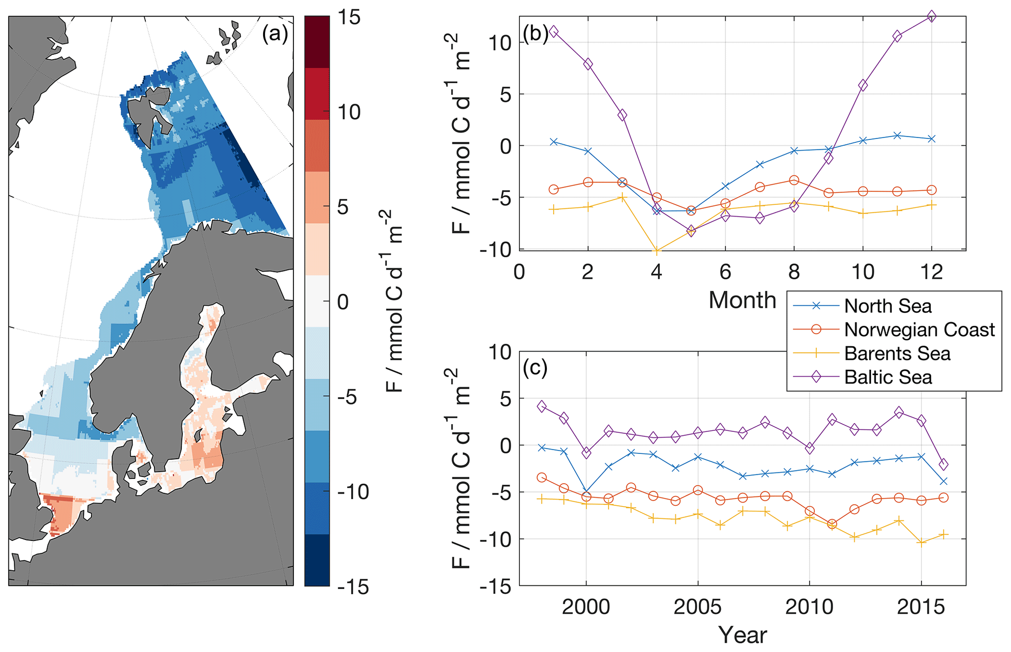
Figure 13The average air–sea CO2 flux over the period 1998–2016 (a, red colors indicate sink regions, while blue colors indicate source regions). For every region average fluxes are show as seasonal averages (b) and time series of annual fluxes (c).
The air–sea CO2 fluxes and their trends (Fig. 13) show that most regions are a net and increasing sink for CO2. The only net source regions are the southern North Sea and the Baltic Sea. The two different regimes in the North Sea, with the southern, nonstratified part being a source and the northern temporarily stratified part a sink for CO2, have been described in the literature before (Thomas et al., 2004), but the gradient between them as represented here may be a too sharp (Sect. 3.1). However, there is a large interannual variability in the fCO2 disequilibrium (Omar et al., 2010), and studies based on different years find conflicting results regarding the direction of the flux (Kitidis et al., 2019; Schiettecatte et al., 2007; Thomas et al., 2004). This large interannual variability was also present in our maps. During some years, larger parts of the North Sea were a net source, while during other years also the southern North Sea acted as net sink (not shown).
The seasonal variations in the air–sea flux are driven by a combination of the changes in the disequilibrium, the wind strength and the ice cover. As there is less wind during summer, when the disequilibrium is large, but a smaller disequilibrium during winter, when the wind strength is high, the seasonal variability in the flux is often less clear than that in the disequilibrium. This can be seen in the Barents Sea and Norwegian Coast. Yasunaka et al. (2018) found the seasonal and interannual variation in the Barents Sea and the Norwegian Sea mostly corresponded to the wind speed and the sea ice concentration. We see the strongest dependence on the air–sea disequilibrium, however (not shown). This indicates that the seasonal and interannual variability in our fCO2 maps is larger than in the maps generated by Yasunaka et al. (2018). Still, our average fluxes fit well with those reported by Yasunaka et al. (2018) of −8 to −12 (Barents Sea) and −4 to −8 (Norwegian Coast). In the North Sea there is almost no net flux during winter, as the surface ocean is more or less in equilibrium with the atmosphere. In the Baltic Sea, there are high fluxes into the atmosphere during winter as here a large oversaturation coincides with strong winds. This is also why the Baltic Sea is a net source region. Although Parard et al. (2017) did find slightly smaller seasonal fluxes (+15 during winter and −8 during summer), the annual air–sea CO2 fluxes are in good agreement (0 to +4 between 1998 and 2011).
The uncertainty in the calculated fluxes is a result of the uncertainties in the fCO2 observations, ΔfCO2 maps, the gas exchange parameterization and the wind product. The uncertainty of the ΔfCO2 is mostly driven by the uncertainty of the MLR, resulting in an error between 12 and 39 µatm, according to the RMSE values of MLR1 for the different regions (Table 5). A number of studies address the uncertainty of gas exchange parameterizations and the wind products (Couldrey et al., 2016; Gregg et al., 2014; Ho and Wanninkhof, 2016). For this study, we apply an uncertainty of the gas transfer velocity of 20 % (Wanninkhof, 2014). This will result in an uncertainty of the air–sea flux of about 2 . It has to be kept in mind that the absolute uncertainty in k increases with increasing wind speed but that the uncertainty in the wind speed has the largest influence in summer when also the disequilibrium is large. In contrast, the uncertainty in ΔfCO2 will cause larger errors in winter, when the wind speeds are high.
There is an ongoing discussion of how and to which extent the dominant climate mode in the North Atlantic, the North Atlantic Oscillation (NAO), is driving the variability in the CO2 fluxes (Salt et al., 2013; Tjiputra et al., 2012; Watson et al., 2009). Even though some features in the time series seem to coincide with very extreme states of the NAO, such as a very large disequilibrium along the Norwegian Coast in 2010, we could not find any significant correlation between the CO2 fluxes and the NAO index.
The MLR approach presented in this work is a relatively easy and straight forward method to produce monthly fCO2 maps with a high spatial resolution in coastal seas, and the use of available open-ocean maps improved the coastal maps significantly. The maps reproduce nicely the main spatial and temporal patterns that are present in observations in the different regions for both fCO2 and pH. The surface seawater fCO2 trends were mostly lower than the atmospheric trends and also lower than the trends found in the open North Atlantic. Results show that the northern European shelf is an increasing net sink for CO2. Only the Baltic Sea is a net source region. This method clearly has the potential to be extended to a larger region. However, it should be handled with care in regions with only a small number of observations as the MLR can lead to unrealistic values.
Long-term observations with a high temporal resolution are extremely important for developing maps such as presented here. While a decent spatial coverage exists for the open North Atlantic, most coastal regions are still undersampled, in particular relative to their high variability in time and space. To further understand and interpret the trends in fCO2 and pH it is necessary to increase our knowledge and understanding of the interaction between primary production, respiration in the water column and the sediments, mixing and gas exchange, and their influence on the carbon cycle.
Besides an increased amount of in situ observations, also improved, higher-resolution driver data hold the potential to enable a better representation of spatial gradients. Including not only satellite-derived chlorophyll data but also colored dissolved organic matter (CDOM) can also lead to an improved performance of the regressions, especially in regions with a high load of terrestrial dissolved organic carbon.
While MLR-derived sea surface fCO2 maps provide a coherent picture of the entire region, they have clear limitations and should be interpreted with caution in regions with few or no observations. A large number of observations is essential both for producing high quality maps and for their validation. Also, observations of a second parameter of the carbon system would be beneficial for deriving pH maps – to reduce and quantify the error introduced by estimating alkalinity from salinity. In addition to that, our work neglects the areas closest to land due to unavailability of CO2 data and reanalysis products in those areas. For adding their contribution to the flux estimates, new platforms specialized on measurements directly at the land–ocean interface need to be developed.
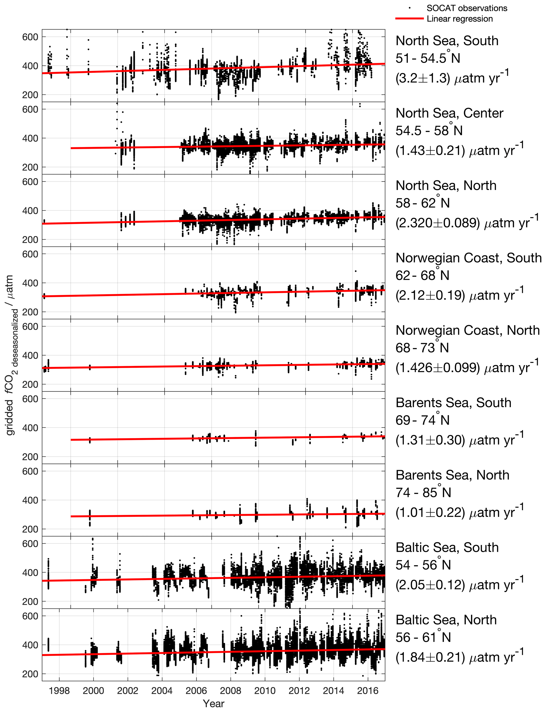
Figure A1Trend in surface ocean fCO2 in deseasonalized, gridded observation data (SOCAT v5).
The dataset is available at https://doi.org/10.18160/939X-PMHU (last access: 9 February 2021).
The supplement related to this article is available online at: https://doi.org/10.5194/bg-18-1127-2021-supplement.
MB performed the MLR and prepared the manuscript with support from all authors. AO provided input to constructing the MLRs. MB, AO, AbO, IS and GR provided pCO2 data and knowledge about the specific coastal areas they are experts in. PL and CR contributed to this work by providing their open-ocean maps and providing support to constructing the MLRs.
The authors declare that they have no conflict of interest.
First of all, we want to thank everyone involved in the collection and quality control of surface ocean CO2 data. The Surface Ocean CO2 Atlas (SOCAT) is an international effort, endorsed by the International Ocean Carbon Coordination Project (IOCCP), the Surface Ocean Lower Atmosphere Study (SOLAS) and the Integrated Marine Biosphere Research (IMBeR) program, to deliver a uniformly quality-controlled surface ocean CO2 database. The many researchers and funding agencies responsible for the collection of data and quality control are thanked for their contributions to SOCAT. We used NCEP Reanalysis 2 data provided by the NOAA/OAR/ESRL PSD, Boulder, Colorado, USA, from their website at https://www.esrl.noaa.gov/psd/ (last access: 12 June 2019). This study has been conducted using EU Copernicus Marine Service Information.
This research has been supported by the Norges Forskningsråd (ICOS Norway, grant no. 245927; Nansen Legacy, grant no. 276730), Horizon 2020 (VERIFY, grant no. 776810), and the Bundesministerium für Bildung und Forschung (BONUS INTEGRAL, grant no. 03F0773A).
This paper was edited by Jack Middelburg and reviewed by two anonymous referees.
Bakker, D. C. E., Pfeil, B., Landa, C. S., Metzl, N., O'Brien, K. M., Olsen, A., Smith, K., Cosca, C., Harasawa, S., Jones, S. D., Nakaoka, S., Nojiri, Y., Schuster, U., Steinhoff, T., Sweeney, C., Takahashi, T., Tilbrook, B., Wada, C., Wanninkhof, R., Alin, S. R., Balestrini, C. F., Barbero, L., Bates, N. R., Bianchi, A. A., Bonou, F., Boutin, J., Bozec, Y., Burger, E. F., Cai, W.-J., Castle, R. D., Chen, L., Chierici, M., Currie, K., Evans, W., Featherstone, C., Feely, R. A., Fransson, A., Goyet, C., Greenwood, N., Gregor, L., Hankin, S., Hardman-Mountford, N. J., Harlay, J., Hauck, J., Hoppema, M., Humphreys, M. P., Hunt, C. W., Huss, B., Ibánhez, J. S. P., Johannessen, T., Keeling, R., Kitidis, V., Körtzinger, A., Kozyr, A., Krasakopoulou, E., Kuwata, A., Landschützer, P., Lauvset, S. K., Lefèvre, N., Lo Monaco, C., Manke, A., Mathis, J. T., Merlivat, L., Millero, F. J., Monteiro, P. M. S., Munro, D. R., Murata, A., Newberger, T., Omar, A. M., Ono, T., Paterson, K., Pearce, D., Pierrot, D., Robbins, L. L., Saito, S., Salisbury, J., Schlitzer, R., Schneider, B., Schweitzer, R., Sieger, R., Skjelvan, I., Sullivan, K. F., Sutherland, S. C., Sutton, A. J., Tadokoro, K., Telszewski, M., Tuma, M., van Heuven, S. M. A. C., Vandemark, D., Ward, B., Watson, A. J., and Xu, S.: A multi-decade record of high-quality fCO2 data in version 3 of the Surface Ocean CO2 Atlas (SOCAT), Earth Syst. Sci. Data, 8, 383–413, https://doi.org/10.5194/essd-8-383-2016, 2016. a, b, c
Bauer, J. E., Cai, W.-J., Raymond, P. A., Bianchi, T. S., Hopkinson, C. S., and Regnier, P. A. G.: The changing carbon cycle of the coastal ocean, Nature, 504, 61–70, https://doi.org/10.1038/nature12857, 2013. a
Blanton, J. O.: Circulation processes along oceanic margins in relation to material fluxes, in: Ocean Margin Processes in Global Change, edited by: Mantoura, R. F. C., Martin, J. M., and Wollast, R., Wiley, New York, 145–63, 1991. a
Borges, A. V. and Gypens, N.: Carbonate chemistry in the coastal zone responds more strongly to eutrophication than ocean acidification, Limnol. Oceanogr., 55, 346–353, https://doi.org/10.4319/lo.2010.55.1.0346, 2010. a
Bourgeois, T., Orr, J. C., Resplandy, L., Terhaar, J., Ethé, C., Gehlen, M., and Bopp, L.: Coastal-ocean uptake of anthropogenic carbon, Biogeosciences, 13, 4167–4185, https://doi.org/10.5194/bg-13-4167-2016, 2016. a
Bricheno, L. M., Wolf, J. M., and Brown, J. M.: Impacts of high resolution model downscaling in coastal regions, Cont. Shelf Res., 87, 7–16, https://doi.org/10.1016/j.csr.2013.11.007, 2014. a
Cai, W.-J., Hu, X., Huang, W.-J., Murrell, M. C., Lehrter, J. C., Lohrenz, S. E., Chou, W.-C., Zhai, W., Hollibaugh, J. T., Wang, Y., Zhao, P., Guo, X., Gundersen, K., Dai, M., and Gong, G.-C.: Acidification of subsurface coastal waters enhanced by eutrophication, Nat. Geosci., 4, 766–770, https://doi.org/10.1038/ngeo1297, 2011. a
Cavalieri, D. J., Parkinson, C. L., Gloersen, P., and Zwally, H. J.: Sea Ice Concentrations from Nimbus-7 SMMR and DMSP SSM/I-SSMIS Passive Microwave Data, Version 1, Monthly, https://doi.org/10.5067/8GQ8LZQVL0VL, NASA National Snow and Ice Data Center Distributed Active Archive Center, Boulder, Colorado USA, 1996. a
Center, N. G. D.: 2-minute Gridded Global Relief Data (ETOPO2) v2, NOAA, https://doi.org/10.7289/V5J1012Q, 2006. a
Cooperative Global Atmospheric Data Integration Project: Multi-laboratory compilation of atmospheric carbon dioxide data for the period 1968-2014, obspack_co2_1_GLOBALVIEWplus_v1.0_2015-07-30, https://doi.org/10.15138/G3RP42, NOAA Earth System Research Laboratory, Global Monitoring Division, 2015. a
Couldrey, M. P., Oliver, K. I. C., Yool, A., Halloran, P. R., and Achterberg, E. P.: On which timescales do gas transfer velocities control North Atlantic CO2 flux variability?, Global Biogeochem. Cy., 30, 787–802, https://doi.org/10.1002/2015GB005267, 2016. a
Desmit, X., Nohe, A., Borges, A. V., Prins, T., Cauwer, K. D., Lagring, R., Van der Zande, D., and Sabbe, K.: Changes in chlorophyll concentration and phenology in the North Sea in relation to de-eutrophication and sea surface warming, Limnol. Oceanogr., 65, 828–847, https://doi.org/10.1002/lno.11351, 2020. a
Dickson, A. and Millero, F.: A comparison of the equilibrium constants for the dissociation of carbonic acid in seawater media, Deep-Sea Res. Pt. I, 34, 1733–1743, https://doi.org/10.1016/0198-0149(87)90021-5, 1987. a
Dickson, A. G.: Standard potential of the reaction: AgCl(s) + 12H2(g) = Ag(s) + HCl(aq), and and the standard acidity constant of the ion HSO4 in synthetic sea water from 273.15 to 318.15 K, J. Chem. Thermodyn., 22, 113–127, https://doi.org/10.1016/0021-9614(90)90074-Z, 1990. a
Fay, A. R. and McKinley, G. A.: Correlations of surface ocean pCO2 to satellite chlorophyll on monthly to interannual timescales, Global Biogeochem. Cy., 31, 436–455, https://doi.org/10.1002/2016GB005563, 2017. a
Fröb, F., Olsen, A., Becker, M., Chafik, L., Johannessen, T., Reverdin, G., and Omar, A.: Wintertime fCO2 Variability in the Subpolar North Atlantic Since 2004, Geophys. Res. Lett., 46, 1580–1590, https://doi.org/10.1029/2018GL080554, 2019. a, b
Gregg, W. W., Casey, N. W., and Rousseaux, C. S.: Sensitivity of simulated global ocean carbon flux estimates to forcing by reanalysis products, Ocean Model., 80, 24–35, https://doi.org/10.1016/j.ocemod.2014.05.002, 2014. a
Griffiths, J. R., Kadin, M., Nascimento, F. J. A., Tamelander, T., Törnroos, A., Bonaglia, S., Bonsdorff, E., Brüchert, V., Gårdmark, A., Järnström, M., Kotta, J., Lindegren, M., Nordström, M. C., Norkko, A., Olsson, J., Weigel, B., Žydelis, R., Blenckner, T., Niiranen, S., and Winder, M.: The importance of benthic–pelagic coupling for marine ecosystem functioning in a changing world, Glob. Change Biol., 23, 2179–2196, https://doi.org/10.1111/gcb.13642, 2017. a
Gruber, N., Clement, D., Carter, B. R., Feely, R. A., Heuven, S. v., Hoppema, M., Ishii, M., Key, R. M., Kozyr, A., Lauvset, S. K., Monaco, C. L., Mathis, J. T., Murata, A., Olsen, A., Perez, F. F., Sabine, C. L., Tanhua, T., and Wanninkhof, R.: The oceanic sink for anthropogenic CO2 from 1994 to 2007, Science, 363, 1193–1199, https://doi.org/10.1126/science.aau5153, 2019. a
Ho, D. T. and Wanninkhof, R.: Air–sea gas exchange in the North Atlantic: 3He/SF6 experiment during GasEx-98, Tellus B, 68, 30198, https://doi.org/10.3402/tellusb.v68.30198, 2016. a
Jones, S. D., Quéré, C. L., Rödenbeck, C., Manning, A. C., and Olsen, A.: A statistical gap-filling method to interpolate global monthly surface ocean carbon dioxide data, J. Adv. Model. Earth Sy., 7, 1554–1575, https://doi.org/10.1002/2014MS000416, 2015. a
Kanamitsu, M., Ebisuzaki, W., Woollen, J., Yang, S.-K., Hnilo, J. J., Fiorino, M., and Potter, G. L.: NCEP–DOE AMIP-II Reanalysis (R-2), B. Am. Meteorol. Soc., 83, 1631–1644, https://doi.org/10.1175/BAMS-83-11-1631, 2002. a
Kitidis, V., Shutler, J. D., Ashton, I., Warren, M., Brown, I., Findlay, H., Hartman, S. E., Sanders, R., Humphreys, M., Kivimäe, C., Greenwood, N., Hull, T., Pearce, D., McGrath, T., Stewart, B. M., Walsham, P., McGovern, E., Bozec, Y., Gac, J.-P., van Heuven, S. M. A. C., Hoppema, M., Schuster, U., Johannessen, T., Omar, A., Lauvset, S. K., Skjelvan, I., Olsen, A., Steinhoff, T., Körtzinger, A., Becker, M., Lefevre, N., Diverrès, D., Gkritzalis, T., Cattrijsse, A., Petersen, W., Voynova, Y. G., Chapron, B., Grouazel, A., Land, P. E., Sharples, J., and Nightingale, P. D.: Winter weather controls net influx of atmospheric CO2 on the north-west European shelf, Sci. Rep.-UK, 9, 20153, https://doi.org/10.1038/s41598-019-56363-5, 2019. a, b, c, d
Landschützer, P., Gruber, N., Bakker, D. C. E., Schuster, U., Nakaoka, S., Payne, M. R., Sasse, T. P., and Zeng, J.: A neural network-based estimate of the seasonal to inter-annual variability of the Atlantic Ocean carbon sink, Biogeosciences, 10, 7793–7815, https://doi.org/10.5194/bg-10-7793-2013, 2013. a
Landschützer, P., Gruber, N., Bakker, D. C. E., and Schuster, U.: Recent variability of the global ocean carbon sink, Global Biogeochem. Cy., 28, 927–949, https://doi.org/10.1002/2014GB004853, 2014. a
Landschützer, P., Gruber, N., and Bakker, D. C. E.: Decadal variations and trends of the global ocean carbon sink, Global Biogeochem. Cy., 30, 1396–1417, https://doi.org/10.1002/2015GB005359, 2016. a, b, c
Landschützer, P., Gruber, N., and Bakker, D. C. E.: An updated observation-based global monthly gridded sea surface pCO2 and air–sea CO2 flux product from 1982 through 2015 and its monthly climatology (NCEI Accession 0160558), Version 2.2, NOAA National Centers for Environmental Information, available at: https://www.ncei.noaa.gov/access/ocean-carbon-data-system/oceans/SPCO2_1982_2015_ETH_SOM_FFN.html (last access: 22 August 2019), 2017. a, b, c, d, e
Landschützer, P., Gruber, N., Bakker, D. C. E., Stemmler, I., and Six, K. D.: Strengthening seasonal marine CO2 variations due to increasing atmospheric CO2, Nat. Clim. Change, 8, 146, https://doi.org/10.1038/s41558-017-0057-x, 2018. a
Landschützer, P., Ilyina, T., and Lovenduski, N. S.: Detecting Regional Modes of Variability in Observation-Based Surface Ocean pCO2, Geophys. Res. Lett., 46, 2670–2679, https://doi.org/10.1029/2018GL081756, 2019. a
Landschützer, P., Laruelle, G. G., Roobaert, A., and Regnier, P.: Landschützer, P., Laruelle, G. G., Roobaert, A., and Regnier, P.: A uniform pCO2 climatology combining open and coastal oceans, Earth Syst. Sci. Data, 12, 2537–2553, https://doi.org/10.5194/essd-12-2537-2020, 2020. a
Laruelle, G. G., Dürr, H. H., Slomp, C. P., and Borges, A. V.: Evaluation of sinks and sources of CO2 in the global coastal ocean using a spatially-explicit typology of estuaries and continental shelves, Geophys. Res. Lett., 37, https://doi.org/10.1029/2010GL043691, 2010. a
Laruelle, G. G., Dürr, H. H., Lauerwald, R., Hartmann, J., Slomp, C. P., Goossens, N., and Regnier, P. A. G.: Global multi-scale segmentation of continental and coastal waters from the watersheds to the continental margins, Hydrol. Earth Syst. Sci., 17, 2029–2051, https://doi.org/10.5194/hess-17-2029-2013, 2013. a
Laruelle, G. G., Landschützer, P., Gruber, N., Tison, J.-L., Delille, B., and Regnier, P.: Global high-resolution monthly pCO2 climatology for the coastal ocean derived from neural network interpolation, Biogeosciences, 14, 4545–4561, https://doi.org/10.5194/bg-14-4545-2017, 2017. a, b
Laruelle, G. G., Cai, W.-J., Hu, X., Gruber, N., Mackenzie, F. T., and Regnier, P.: Continental shelves as a variable but increasing global sink for atmospheric carbon dioxide, Nat. Commun., 9, 454, https://doi.org/10.1038/s41467-017-02738-z, 2018. a, b, c, d, e
Lauvset, S. K. and Gruber, N.: Long-term trends in surface ocean pH in the North Atlantic, Mar. Chem., 162, 71–76, https://doi.org/10.1016/j.marchem.2014.03.009, 2014. a, b
Lauvset, S. K., Gruber, N., Landschützer, P., Olsen, A., and Tjiputra, J.: Trends and drivers in global surface ocean pH over the past 3 decades, Biogeosciences, 12, 1285–1298, https://doi.org/10.5194/bg-12-1285-2015, 2015. a, b
Lima, F. P. and Wethey, D. S.: Three decades of high-resolution coastal sea surface temperatures reveal more than warming, Nat. Commun., 3, 1–13, https://doi.org/10.1038/ncomms1713, 2012. a
Lind, S., Ingvaldsen, R. B., and Furevik, T.: Arctic warming hotspot in the northern Barents Sea linked to declining sea-ice import, Nat. Clim. Change, 8, 634–639, https://doi.org/10.1038/s41558-018-0205-y, 2018. a
Locarnini, R., Mishonov, A., Baranova, O., Boyer, T., Zweng, M., GarciA, H., Reagan, J., Seidov, D., Weathers, K., Paver, C., and Smoylar, I.: World Ocean Atlas 2018, Volume 1: Temperature, Technical Ed.: Mishonov, A., NOAA Atlas NESDIS 81, 52 pp., 2018. a
Loose, B., McGillis, W. R., Schlosser, P., Perovich, D., and Takahashi, T.: Effects of freezing, growth, and ice cover on gas transport processes in laboratory seawater experiments, Geophys. Res. Lett., 36, https://doi.org/10.1029/2008GL036318, 2009. a
Mehrbach, C., Culberson, C., Hawley, J., and Pytkowicz, R.: Measurement of the apparent dissociation constants of carbonic acid in seawater at atmospheric pressure, Limnol. Oceanogr., 18, 897–907, 1973. a
Meyer, M., Pätsch, J., Geyer, B., and Thomas, H.: Revisiting the Estimate of the North Sea Air–Sea Flux of CO2 in 2001/2002: The Dominant Role of Different Wind Data Products, J. Geophys. Res.-Biogeo., 123, 1511–1525, https://doi.org/10.1029/2017JG004281, 2018. a
Müller, J. D., Schneider, B., and Rehder, G.: Long-term alkalinity trends in the Baltic Sea and their implications for CO2-induced acidification, Limnol. Oceanogr., 61, 1984–2002, https://doi.org/10.1002/lno.10349, 2016. a, b
Naegler, T.: Reconciliation of excess 14C-constrained global CO2 piston velocity estimates, Tellus B, 61, 372–384, https://doi.org/10.1111/j.1600-0889.2008.00408.x, 2009. a
Nondal, G., Bellerby, R. G. J., Oldenc, A., Johannessena, T., and Olafssond, J.: Optimal evaluation of the surface ocean CO2 system in the northern North Atlantic using data from voluntary observing ships, Limnol. Oceanogr., 7, 109–118, 2009. a, b
Omar, A. M., Olsen, A., Johannessen, T., Hoppema, M., Thomas, H., and Borges, A. V.: Spatiotemporal variations of fCO2 in the North Sea, Ocean Sci., 6, 77–89, https://doi.org/10.5194/os-6-77-2010, 2010. a
Omar, A. M., Thomas, H., Olsen, A., Becker, M., Skjelvan, I., and Reverdin, G.: Trend of ocean acidification and pCO2 in the northern North Sea, 2004–2015, J. Geophys. Res.-Biogeo., 124, 3088–3103, 2019. a, b, c, d, e
Oziel, L., Neukermans, G., Ardyna, M., Lancelot, C., Tison, J.-L., Wassmann, P., Sirven, J., Ruiz-Pino, D., and Gascard, J.-C.: Role for Atlantic inflows and sea ice loss on shifting phytoplankton blooms in the Barents Sea, J. Geophys. Res.-Oceans, 5121–5139, https://doi.org/10.1002/2016JC012582, 2017. a, b
Parard, G., Charantonis, A. A., and Rutgersson, A.: Using satellite data to estimate partial pressure of CO2 in the Baltic Sea, J. Geophys. Res.-Biogeo., 121, 1002–1015, https://doi.org/10.1002/2015JG003064, 2016. a, b
Parard, G., Rutgersson, A., Raj Parampil, S., and Charantonis, A. A.: The potential of using remote sensing data to estimate air–sea CO2 exchange in the Baltic Sea, Earth Syst. Dynam., 8, 1093–1106, https://doi.org/10.5194/esd-8-1093-2017, 2017. a, b, c
Pierrot, D., Neill, C., Sullivan, K., Castle, R., Wanninkhof, R., Lüger, H., Johannessen, T., Olsen, A., Feely, R. A., and Cosca, C. E.: Recommendations for autonomous underway pCO2 measuring systems and data-reduction routines, Deep-Sea Res. Pt. II, 56, 512–522, https://doi.org/https://doi.org/10.1016/j.dsr2.2008.12.005, 2009. a
Rödenbeck, C., Keeling, R. F., Bakker, D. C. E., Metzl, N., Olsen, A., Sabine, C., and Heimann, M.: Global surface-ocean pCO2 and sea–air CO2 flux variability from an observation-driven ocean mixed-layer scheme, Ocean Sci., 9, 193–216, https://doi.org/10.5194/os-9-193-2013, 2013. a
Rödenbeck, C., Bakker, D. C. E., Metzl, N., Olsen, A., Sabine, C., Cassar, N., Reum, F., Keeling, R. F., and Heimann, M.: Interannual sea–air CO2 flux variability from an observation-driven ocean mixed-layer scheme, Biogeosciences, 11, 4599–4613, https://doi.org/10.5194/bg-11-4599-2014, 2014. a, b, c
Rödenbeck, C., Bakker, D. C. E., Gruber, N., Iida, Y., Jacobson, A. R., Jones, S., Landschützer, P., Metzl, N., Nakaoka, S., Olsen, A., Park, G.-H., Peylin, P., Rodgers, K. B., Sasse, T. P., Schuster, U., Shutler, J. D., Valsala, V., Wanninkhof, R., and Zeng, J.: Data-based estimates of the ocean carbon sink variability – first results of the Surface Ocean pCO2 Mapping intercomparison (SOCOM), Biogeosciences, 12, 7251–7278, https://doi.org/10.5194/bg-12-7251-2015, 2015. a, b
Roobaert, A., Laruelle, G. G., Landschützer, P., and Regnier, P.: Uncertainty in the global oceanic CO2 uptake induced by wind forcing: quantification and spatial analysis, Biogeosciences, 15, 1701–1720, https://doi.org/10.5194/bg-15-1701-2018, 2018. a
Salt, L. A., Thomas, H., Prowe, A. E. F., Borges, A. V., Bozec, Y., and de Baar, H. J. W.: Variability of North Sea pH and CO2 in response to North Atlantic Oscillation forcing, J. Geophys. Res.-Biogeo., 118, 1584–1592, https://doi.org/10.1002/2013JG002306, 2013. a, b, c, d, e
Schiettecatte, L. S., Thomas, H., Bozec, Y., and Borges, A. V.: High temporal coverage of carbon dioxide measurements in the Southern Bight of the North Sea, Mar. Chem., 106, 161–173, https://doi.org/10.1016/j.marchem.2007.01.001, 2007. a
Schneider, B. and Müller, J. D.: Biogeochemical Transformations in the Baltic Sea: Observations Through Carbon Dioxide Glasses, Springer Oceanography, Springer International Publishing, 2018. a, b
Sharples, J., Ross, O. N., Scott, B. E., Greenstreet, S. P. R., and Fraser, H.: Inter-annual variability in the timing of stratification and the spring bloom in the North-western North Sea, Cont. Shelf Res., 26, 733–751, https://doi.org/10.1016/j.csr.2006.01.011, 2006. a
Thomas, H., Bozec, Y., Elkalay, K., and de Baar, H. J. W.: Enhanced Open Ocean Storage of CO2 from Shelf Sea Pumping, Science, 304, 1005–1008, https://doi.org/10.1126/science.1095491, 2004. a, b
Thomas, H., Friederike Prowe, A. E., van Heuven, S., Bozec, Y., de Baar, H. J. W., Schiettecatte, L.-S., Suykens, K., Koné, M., Borges, A. V., Lima, I. D., and Doney, S. C.: Rapid decline of the CO2 buffering capacity in the North Sea and implications for the North Atlantic Ocean, Global Biogeochem. Cy., 21, https://doi.org/10.1029/2006GB002825, 2007. a, b
Tjiputra, J. F., Olsen, A., Assmann, K., Pfeil, B., and Heinze, C.: A model study of the seasonal and long–term North Atlantic surface pCO2 variability, Biogeosciences, 9, 907–923, https://doi.org/10.5194/bg-9-907-2012, 2012. a
Uppström, L. R.: The boron/chlorinity ratio of deep-sea water from the Pacific Ocean, Deep Sea Research and Oceanographic Abstracts, 21, 161–162, https://doi.org/10.1016/0011-7471(74)90074-6, 1974. a
van Heuven, S., Pierrot, D., Lewis, E., and Wallace, D.: MATLAB Program Developed for CO2 System Calculations, ORNL/CDIAC-105b, Carbon Dioxide Information Analysis Center, Oak Ridge National Laboratory, U.S. Department of Energy, Oak Ridge, Tennessee, 2009. a
Wanninkhof, R.: Relationship between wind speed and gas exchange over the ocean revisited: Gas exchange and wind speed over the ocean, Limnol. Oceanogr.-Meth., 12, 351–362, https://doi.org/10.4319/lom.2014.12.351, 2014. a, b, c
Watson, A. J., Schuster, U., Bakker, D. C. E., Bates, N. R., Corbiere, A., Gonzalez-Davila, M., Friedrich, T., Hauck, J., Heinze, C., Johannessen, T., Kortzinger, A., Metzl, N., Olafsson, J., Olsen, A., Oschlies, A., Padin, X. A., Pfeil, B., Santana-Casiano, J. M., Steinhoff, T., Telszewski, M., Rios, A. F., Wallace, D. W. R., and Wanninkhof, R.: Tracking the Variable North Atlantic Sink for Atmospheric CO2, Science, 326, 1391–1393, 2009. a
Weiss, R. F.: Carbon dioxide in water and seawater: The solubility of a non-ideal gas, Mar. Chem., 2, 203–215, 1974. a
Wesslander, K., Omstedt, A., and Schneider, B.: Inter-annual and seasonal variations in the air–sea CO2 balance in the central Baltic Sea and the Kattegat, Cont. Shelf Res., 30, 1511–1521, 2010. a
Wollast, R.: Evaluation and comparison of the global carbon cycle in the coastal zone and in the open ocean, in: The Sea, edited by: Brink, K. H. and Robinson, A. R., John Wiley & Sons, New York, 213–252, 1998. a
Yasunaka, S., Siswanto, E., Olsen, A., Hoppema, M., Watanabe, E., Fransson, A., Chierici, M., Murata, A., Lauvset, S. K., Wanninkhof, R., Takahashi, T., Kosugi, N., Omar, A. M., van Heuven, S., and Mathis, J. T.: Arctic Ocean CO2 uptake: an improved multiyear estimate of the air–sea CO2 flux incorporating chlorophyll a concentrations, Biogeosciences, 15, 1643–1661, https://doi.org/10.5194/bg-15-1643-2018, 2018. a, b, c, d, e, f, g, h, i