the Creative Commons Attribution 4.0 License.
the Creative Commons Attribution 4.0 License.
 | 04 Jan 2021
Calculating canopy stomatal conductance from eddy covariance measurements, in light of the energy budget closure problem
Scott R. Saleska
Canopy stomatal conductance is commonly estimated from eddy covariance measurements of the latent heat flux (LE) by inverting the Penman–Monteith equation. That method ignores eddy covariance measurements of the sensible heat flux (H) and instead calculates H implicitly as the residual of all other terms in the site energy budget. Here we show that canopy stomatal conductance is more accurately calculated from eddy covariance (EC) measurements of both H and LE using the flux–gradient equations that define conductance and underlie the Penman–Monteith equation, especially when the site energy budget fails to close due to pervasive biases in the eddy fluxes and/or the available energy. The flux–gradient formulation dispenses with unnecessary assumptions, is conceptually simpler, and is as or more accurate in all plausible scenarios. The inverted Penman–Monteith equation, on the other hand, contributes substantial biases and erroneous spatial and temporal patterns to canopy stomatal conductance, skewing its relationships with drivers such as light and vapor pressure deficit.
- Article
(2464 KB) - Full-text XML
- BibTeX
- EndNote


Leaf stomata are a key coupling between the terrestrial carbon and water cycles. They are a gateway for carbon dioxide and transpired water and often limit both at the ecosystem scale (Jarvis and McNaughton, 1986). Although the many stomata in a plant canopy experience a wide range of micro-environmental conditions and therefore exhibit a wide range of behaviors at any given moment in time, it has proven useful in many contexts to approximate the canopy as a single “big leaf” with a single stoma (Baldocchi et al., 1991; Wohlfahrt et al., 2009; Wehr et al., 2017). That stoma is characterized by the canopy stomatal conductance to water vapor (gsV), which can be defined as the total canopy transpiration divided by the transpiration-weighted average water vapor gradient across the many real stomata. This canopy stomatal conductance is not a simple sum of the individual leaf-level conductances and does not vary with time or environment in quite the same way as they do (Baldocchi et al., 1991); it is impacted, for example, by changes in the distribution of light within the canopy.
When the aerodynamic conductance to water vapor outside the leaf (gaV) is greater than gsV, the latter exerts a strong influence on transpiration, from which it can be inferred. The standard method is to calculate gsV from eddy covariance (EC) measurements of the latent heat flux (LE) via the inverted Penman–Monteith (iPM) equation (Monteith, 1965; Grace et al., 1995) – but the EC method and the iPM equation make a strange pairing. The original (not inverted) Penman–Monteith equation was designed to estimate transpiration from the available energy (A), the vapor pressure deficit, and the stomatal and aerodynamic conductances. It was derived from simple flux–gradient relationships for LE and for the sensible heat flux (H) but was formulated in terms of A and LE rather than H and LE. Thus the inverted PM equation estimates gsV from A and LE rather than from H and LE. EC sites, in contrast, measure H and LE but rarely assess A in its entirety. True A is net radiation (Rn) minus heat flux to the deep soil (G), minus heat storage (S) in the shallow soil, canopy air, and biomass. In wetland ecosystems, heat flux by groundwater discharge (W) can also be important (Reed et al., 2018). While net radiation measurements are ubiquitous at EC sites, ground heat flux measurements are less common (Stoy et al., 2013; Purdy et al., 2016) and heat storage and discharge measurements are rare (Lindroth et al., 2010; Reed et al., 2018). As such it is common practice to simply omit S and W and sometimes G from A in the iPM equation.
In general, neither S nor G is negligible. Insufficient measurement of S in particular has been shown (Lindroth et al., 2010; Leuning et al., 2012) to be a major contributor to the infamous energy budget closure problem at EC sites, which is that the measured turbulent heat flux H+LE is about 20 % less than the measured available energy Rn−G on average across the FLUXNET EC site network (Wilson et al., 2002; Foken, 2008; Franssen et al., 2010; Leuning et al., 2012; Stoy et al., 2013). The other major contributor, which also impacts the iPM equation, is systematic underestimation of H+LE by the EC method, probably due to its failure to capture sub-mesoscale transport (Foken, 2008; Stoy et al., 2013; Charuchittipan et al., 2014; Gatzsche et al., 2018; Mauder et al., 2020). Leuning et al. (2012) assessed the relative contributions of S and H+LE to the closure problem using the fact that S largely averages out over 24 h while Rn, H, and LE do not; thus S contributes to the hourly but not the daily energy budget (Lindroth et al., 2010; Leuning et al., 2012). Analyzing over 400 site years of data, they found that the median slope of H+LE versus Rn−G was only 0.75 when plotting hourly averages but went up to 0.9 when plotting daily averages. This result suggests that for the average FLUXNET site, 60 % of the energy budget gap is attributable to S and 40 % to H+LE. Depending on the depth at which G is measured (which is not standard), G might also average down considerably over 24 h and thereby share some of the 60 % attributed to S. Conversely, the part of G that does not average out over 24 h might share some of the 40 % attributed to H+LE, as might Rn and W. Part of that 40 % might also be due to mismatch between the view of the net radiometer and the flux footprint of the eddy covariance tower. But S and H+LE are the most likely sources of large systematic bias across sites.
The iPM equation is further impacted by how the underestimation of H+LE is partitioned between H and LE. While some studies have reported that underestimation of H+LE roughly preserves the Bowen ratio (), others have reported that the failure to capture sub-mesoscale transport causes EC to underestimate H more than LE (Mauder et al., 2020) – a situation that would benefit the iPM equation. Charuchittipan et al. (2014) quantified the preferential underestimation of H relative to LE using a simple formula based on the buoyancy flux, and a study of tall vegetation suggested that the formula holds when B is high (B>2) but that B is instead preserved when it is low or moderate (B<1.5) (Gatzsche et al., 2018). In the latest review of the issue, Mauder et al. (2020) concluded that recent evidence “tends towards a partitioning somewhere between a buoyancy-flux-based and a Bowen-ratio-preserving” one.
To deal with the energy budget closure problem, Wohlfahrt et al. (2009) considered various schemes for correcting the fluxes in the iPM equation, following earlier recommendations that EC fluxes be corrected to close the energy budget in a more general context (Twine et al., 2000). All but one of the schemes in Wohlfahrt et al. (2009) involve attributing the half-hourly budget gap entirely to A or entirely to H+LE, neither of which is generally realistic according to the subsequent results of Leuning et al. (2012), mentioned above. The remaining option from Wohlfahrt et al. (2009) increases H and LE to close the long-term (e.g., daily or monthly) budget gap while preserving the Bowen ratio (B), which is in line with Leuning et al. (2012) in that it attributes the long-term gap to EC and the remaining gap to storage.
Here we use data simulations to show that regardless of whether the energy budget gap is due to A or H+LE, and regardless of how the EC bias is partitioned between the buoyancy flux and Bowen ratio limits, stomatal conductance is more accurately obtained by direct application of the two simple flux–gradient (FG) equations on which the iPM equation is based than by use of the iPM equation itself. By using simulations, we can know the “true” target values and hence the absolute biases in gsV. We also use our simulations to test the effects of perfect and imperfect eddy flux corrections and of bias in the aerodynamic conductance outside the leaf. Lastly, we leave the simulations behind and show how the discrepancy between the FG and iPM formulations impacts the retrieval of gsV over time using real measurements from a conifer forest. We present the FG and iPM formulations in Sect. 2, describe our methods for comparing them in Sect. 3, and report our findings in Sect. 4.
By definition, conductance is the proportionality coefficient between a flux and its driving gradient. In the case of gsV, the flux is transpiration and the gradient is the vapor pressure differential across the “big-leaf” stoma. It is therefore relatively straightforward to calculate gsV from the flux–gradient (FG) equations for transpiration and sensible heat (Baldocchi et al., 1991), rearranged as follows (Wehr and Saleska, 2015):
where rsV (s m−1) is the stomatal resistance to water vapor, raV is the aerodynamic resistance to water vapor (s m−1), raH is the aerodynamic resistance to heat (s m−1), E is the flux of transpired water vapor (mol m−2 s−1), H is the sensible heat flux (W m−2), Ta is the air temperature (K), TL is the effective canopy-integrated leaf temperature (K), ρa is the density of (wet) air (kg m−3), cp is the specific heat capacity of (wet) air (J kg−1 K−1), ea is the vapor pressure in the air (Pa), es(TL) is the saturation vapor pressure inside the leaf as a function of TL (Pa), and R is the molar gas constant (8.314472 J mol−1 K−1). The equation for the saturation vapor pressure (Pa) as a function of temperature (K) is (World Meteorological Organization, 2008)
The aerodynamic resistances describe the path between the surface of the big leaf and whatever reference point in the air at which Ta, ea, ρa, and cp are measured. If that reference point is the top of an eddy flux tower, then that path includes the leaf boundary layer (through which transport is quasi-diffusive) as well as the canopy airspace and some above-canopy air (through which transport is turbulent). The turbulent eddy resistance (re) may be calculated by various methods that do not agree particularly well with one another (e.g., see Baldocchi et al., 1991; Grace et al., 1995; Wehr and Saleska, 2015) but is typically small in “rough surface” ecosystems like forests during the daytime, when raH and raV tend to be dominated by the leaf boundary layer resistances rbH and rbV. An empirical model such as the one given in the Appendix can be used to calculate rbH as a function of wind speed and other variables. Using that model in a temperate deciduous forest, rbH was found to vary only between 8 and 12 s m−1 (Wehr and Saleska, 2015), and so we simply take it to be constant at 10 s m−1 here. The corresponding resistance to water vapor transport can be calculated from rbH via (Hicks et al., 1987)
where Sc is the Schmidt number for water vapor (0.67), Pr is the Prandtl number for air (0.71), and f is the fraction of the leaf surface area that contains stomata (f=0.5 for hypostomatous leaves, which have stomata on only one side, and f=1 for amphistomatous leaves, which have stomata on both sides). The aerodynamic resistances to sensible heat and water vapor are then and .
Finally, the stomatal conductance to water vapor (mol m−2 s−1) is obtained from rsV by (Grace et al., 1995):
where P is the atmospheric pressure.
The above FG theory is also the basis of the Penman–Monteith equation for a leaf (Monteith, 1965) and its inverted form (Grace et al., 1995), which can be expressed as
where LEtr is the latent heat flux associated with transpiration (W m−2), LEev is the latent heat flux associated with evaporation that does not pass through the stomata (W m−2), es(Ta) is the saturation vapor pressure of the air as a function of Ta (Pa) rather than TL, s is the slope of the es curve at Ta (Pa K−1), and γ is the psychrometric constant at Ta (Pa K−1). Rn, G, S, and W also have units of watts per square meter. Latent heat flux is water vapor flux (E) times the latent heat of vaporization of water (about 44.1×10³ J mol−1).
The inverted PM equation is usually expressed in a slightly simpler form by neglecting the distinctions (a) between transpiration and evaporation and (b) between the leaf boundary layer resistances to heat and water vapor. We retain those distinctions here in order to highlight two important points.
-
Absent a means to accurately partition the measured eddy flux of water vapor into transpiration and non-stomatal evaporation (e.g., from soil or wet leaves), the FG and iPM equations are applicable only when evaporation is negligible, which is a difficult situation to verify but does occur at particular times in particular ecosystems (see, e.g., Wehr et al., 2017).
-
Setting rbV=rbH instead of using Eq. (4) is a good approximation for amphistomatous leaves (stomata on both sides) but a poor approximation for the more common hypostomatous leaves (stomata on only one side) (Schymanski and Or, 2017). Indeed, we find that if rbV is set equal to rbH for hypostomatous leaves, the iPM equation underestimates gsV by about 10 % (depending on the relative resistances of the stomata and boundary layer) even when the site energy budget is closed.
Note that the iPM equation can be derived from the FG equations by invoking energy balance to replace H with A−LE in Eq. (2) and then linearizing the Clausius–Clapeyron relation to eliminate leaf temperature:
This psychrometric approximation has been shown to cause significant bias and incorrect limiting behavior in the Penman–Monteith equation (McColl, 2020). McColl (2020) derived a similar, alternative equation that remedies those problems but still uses measurements of A instead of H. The psychrometric approximation and the substitution for H are the only two differences between the FG and iPM formulations. Both formulations rely on the same water flux measurements to estimate transpiration, both approximate the canopy as a big leaf, and both use the same estimate of aerodynamic resistance.
Our analysis consisted of two parts: simulations and real data analysis. The simulations were designed to unambiguously demonstrate the impact of flux measurement biases and the resultant energy budget gap on FG and iPM calculations of gsV, as well as to test the sensitivity of gsV to bias in the estimated aerodynamic resistance outside the leaf; they are described in Sect. 3.1. The real data analysis was designed to assess the magnitude and temporal variation in the discrepancy between the FG and iPM formulations in a real forest and is described in Sect. 3.2.
3.1 Simulations
We assessed the proportional bias in gsV calculated via the iPM and FG formulations by simulating observations and using them to estimate gsV. The simulations were of three snapshots in time roughly typical of midday in three different ecosystems: a temperate deciduous forest in July (the Harvard Forest in Massachusetts, USA; Wehr et al., 2017), a tropical rainforest in May (the Reserva Jaru in Rondônia, Brazil; Grace et al., 1995), and a tropical savannah in September (Virginia Park in Queensland, Australia; Leuning et al., 2005). The purpose of including three different ecosystems was to test the FG and iPM formulations across a broad range of environmental and biological input variables (especially Bowen ratios), not to provide a lookup table of quantitative gsV corrections for other sites. The particular sites and time periods within each ecosystem were chosen merely for convenience, as the requisite variables were readily obtainable from the literature or from our past work.
The simulations began by setting the “true” target values of all the variables involved; in other words, their values without any simulated measurement error. To keep these values realistic, we started with approximate observed fluxes and conditions obtained from the papers cited above or from our own work at the Harvard Forest (Table 1), with the precise values of H and LE chosen to satisfy B and energy balance. These fluxes and conditions were then used to calculated the true target gsV using the FG equations (Eqs. 1–5). As the fluxes in Table 1 close the energy budget perfectly, the FG and iPM equations are interchangeable for this step of the simulations apart from the psychrometric approximation (Eq. 7), which causes a small but significant (∼ 5 %) positive bias in iPM-derived gsV. That bias is the reason why iPM-derived gsV does not quite converge on the true value even when the entire energy budget gap is due to the EC fluxes and those fluxes are perfectly corrected (see Fig. 2). Thus we could have instead used the iPM equation (Eq. 6) to set the true gsV and obtained similar results, except that the psychrometric approximation bias would have appeared, incorrectly, to afflict the FG results instead of the iPM results.
Table 1Values of environmental and biological variables used in the error simulations (representing midday).
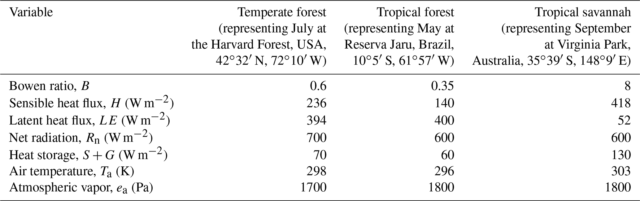
For all sites, W=0 W m−2, rbH=10 s m−1, re=0 s m−1, P=101 325 Pa, and f=0.5.
Next, we simulated a wide range of measurement bias scenarios, each with a 20 % gap in the energy budget (the FLUXNET average). The simulations were explored along three main axes of variation.
-
Variation 1. The energy budget gap was variously apportioned between measurement bias in A and measurement bias in H+LE. The measurement bias in H+LE was applied proportionally to H and LE so as to preserve the true Bowen ratio. All other variables were unbiased.
-
Variation 2. Measurements of H and LE biased the Bowen ratio by varying amounts while the apportioning of the energy budget gap between A and H+LE was fixed at the FLUXNET average (60 % A, 40 % H+LE). All other variables were unbiased.
-
Variation 3. Estimates of the aerodynamic conductance outside the leaf were biased by varying amounts while the apportioning of the energy budget gap between A and H+LE was fixed at the FLUXNET average and the measurements of H and LE preserved the true Bowen ratio. All other variables were unbiased.
For each measurement bias scenario, we used the FG and iPM formulations to calculate gsV from the simulated (usually erroneous) eddy flux measurements, from perfectly corrected eddy flux measurements, and from eddy flux measurements adjusted to close the long-term energy budget while preserving the Bowen ratio, as proposed in Wohlfahrt et al. (2009). In our simulations of a single point in time, the latter adjustment was represented by increasing H and LE proportionally such that H+LE became equal to the true value of A. Such an adjustment restores the true eddy fluxes if their measurements did not bias the Bowen ratio and was therefore redundant with the perfect correction for Variation 1 and Variation 3. Conversely, the perfect correction was of no interest for Variation 2, as it removes all bias in the Bowen ratio.
3.2 Analysis of real measured time series
In order to show how the FG and iPM methods differ in a real forest over the diurnal cycle, we calculated time series of gsV from real hourly measurements at Howland Forest recorded in the AmeriFlux EC site database (Site US-Ho1; Hollinger, 1996). Howland Forest is a mostly coniferous forest in Maine, USA (45∘12′ N, 68∘44′ W), which we chose for its intermediate Bowen ratio, for variety, and otherwise for convenience. In addition to using the original measured fluxes, we also calculated gsV after adjusting the eddy fluxes using the long-term energy budget closure scheme proposed by Wohlfahrt et al. (2009) – the same flux adjustment scheme we tested in our simulations. For this scheme at Howland Forest, we computed the slope of H+LE versus Rn−G from a plot of all 24 h averages in the summer of 2014 and then divided both H and LE by that slope.
To minimize the influence of non-stomatal evaporation, we focused on 2 sunny midsummer days more than 24 h after the last rain (25–26 July 2014). Because our aim was to show the relative bias between the FG and iPM methods rather than to obtain the most accurate possible estimate of gsV, we used the constant and roughly appropriate values rbH=10 s m−1 and re=0 as in our simulations, rather than calculating values for these aerodynamic resistances from the data according to models like that in the Appendix. Given that conifer forests are very rough surfaces and that the two daylight periods under consideration were windy with strong turbulent mixing (wind speed >3 m s−1 and friction velocity >0.6 m s−1 from late morning through late afternoon), it is almost certain that the aerodynamic resistance was much less than the stomatal resistance and therefore that the FG and iPM equations were insensitive to rbH and re (see Sect. 4.1).
4.1 Absolute biases revealed by simulations
Our simulations indicate that the flux–gradient formulation is substantially more accurate than the inverted Penman–Monteith equation regardless of the cause and magnitude of the energy budget gap and regardless of the ecosystem type.
Figure 1 shows bias in gsV versus the relative contribution of eddy flux bias to the hourly energy budget gap (the remainder of the gap being due to bias in the available energy). This figure follows Variation 1 from Sect. 3.1, which assumes that eddy flux measurements preserve the true Bowen ratio. Here the FG formulation (solid black lines) is always more accurate than the iPM formulation (solid red lines) because regardless of whether the gap is due to negative measurement bias in A or in H+LE, the iPM equation implicitly overestimates H (as the residual of the other fluxes) and therefore the leaf temperature and therefore the water vapor gradient, which exacerbates underestimation of the conductance. In other words, it is better to have both LE and H underestimated (as in the FG equations) than to have LE underestimated and H overestimated (as in the iPM equation). The dashed lines in Fig. 1 show results calculated using eddy fluxes that have been corrected back to the true values (as studies have aimed to do), in which case the FG formulation becomes unbiased while the iPM equation still suffers from bias in A and from the psychrometric approximation. Figure 2 clarifies the contributions of LE, A, and the psychrometric approximation (Eq. 7) to bias in the iPM equation.
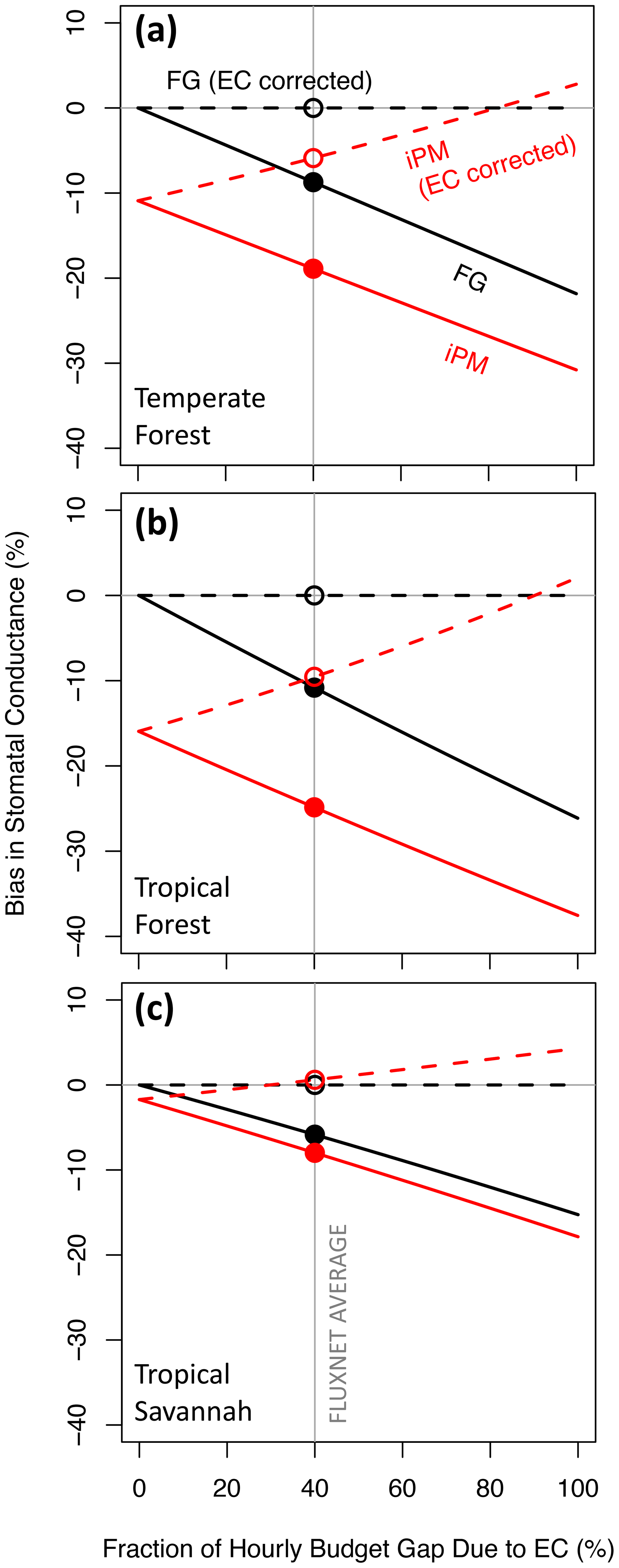
Figure 1Proportional bias in canopy stomatal conductance obtained from the flux–gradient (FG, black) and inverted Penman–Monteith (iPM, red) formulations versus the fraction of the hourly energy budget gap caused by bias in the eddy fluxes rather than by bias in the available energy. Solid lines show results without eddy flux correction and dashed lines show results with perfectly corrected eddy fluxes. The average estimated contribution of eddy flux bias to the budget gap across FLUXNET is indicated by the grey vertical line (Leuning et al., 2012). Circles highlight where the various lines cross the FLUXNET average.
Comparison of Fig. 1a, b, and c reveals that the qualitative relationships in Fig. 1 do not depend on the values of the environmental and biological variables in Table 1, but the severity of the bias in gsV does. The bias in gsV is also proportional to the relative energy budget gap, i.e., (), and will therefore be larger (smaller) than shown here at sites with gaps larger (smaller) than 20 %. Because the bias in gsV varies with environmental and biological site characteristics, it will lead to erroneous spatial patterns in gsV and to erroneous relationships with potential drivers.
As noted in the introduction, pervasive eddy flux biases likely preserve the true Bowen ratio in some but not all circumstances. Thus Fig. 3 shows bias in gsV versus bias in the measured Bowen ratio. This figure follows Variation 2 from Sect. 3.1, which assumes that 40 % of the energy budget gap is due to the eddy fluxes (which is the FLUXNET average). The FG formulation (solid black lines) remains more accurate than the iPM equation (solid red lines) everywhere between the buoyancy-flux-based and Bowen-ratio-preserving limits, except very close to the buoyancy-flux-based limit in the high-B tropical savannah. The iPM equation becomes nearly unbiased in that situation because its inherent assumption that the energy budget gap is due entirely to H becomes nearly true; moreover, the small remaining bias due to underestimation of LE is offset by bias from the psychrometric approximation, which has the opposite sign (see Fig. 2). The dotted lines in Fig. 3 show results calculated using eddy fluxes that have been adjusted to close the long-term energy budget while preserving the (erroneously measured) Bowen ratio (if the eddy fluxes were perfectly corrected as in Fig. 1, there would be no variation along the abscissa for any method in this figure). We include this mis-correction because it is the most likely adjustment to be applied to eddy fluxes in practice, whether it is appropriate or not. It favors the FG formulation when the Bowen ratio bias is small and begins to favor the iPM equation as that bias increases – and it illustrates how improper correction of the eddy fluxes can make the bias in gsV worse.
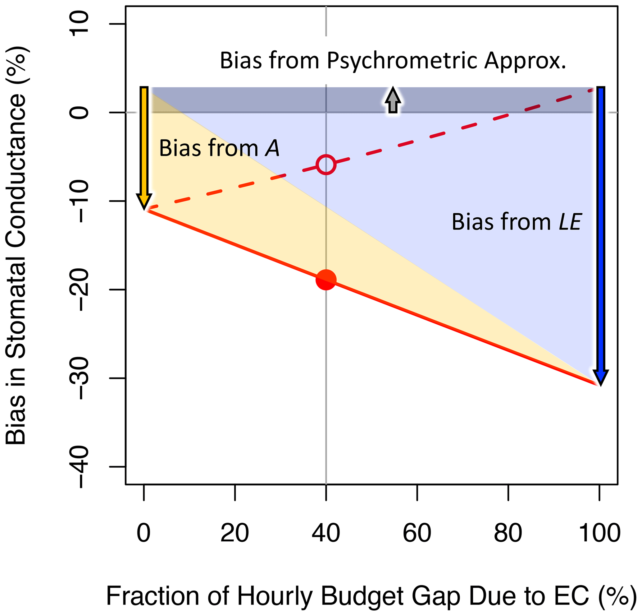
Figure 2Inverted Penman–Monteith results from Fig. 1a, annotated to indicate the various sources of bias.
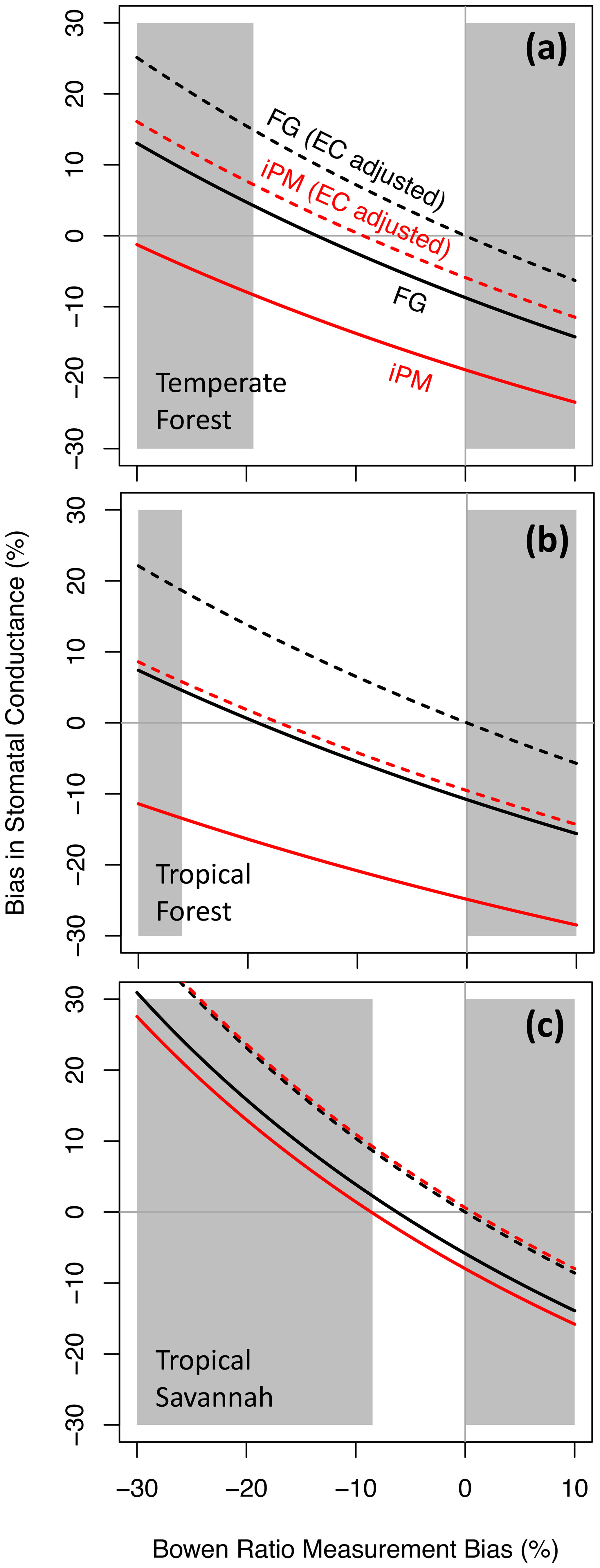
Figure 3Proportional bias in canopy stomatal conductance obtained from the flux–gradient (FG, black) and inverted Penman–Monteith (iPM, red) formulations versus proportional bias in the measured Bowen ratio. Solid lines show results without eddy flux correction, and dotted lines show results with the eddy fluxes adjusted to close the long-term energy budget while preserving the (erroneously measured) Bowen ratio. The unshaded region denotes the plausible range of pervasive bias, which is bounded by the buoyancy-flux-based and Bowen-ratio-preserving limits (see text).
Aside from the energy budget gap, another potentially important source of bias in the FG and iPM equations is the aerodynamic resistance ( and ). Estimates of the aerodynamic resistance come from models of the leaf boundary layer (such as that in the Appendix) and of micrometeorology (see Baldocchi et al., 1991). These models are based on established theory and careful experiments but involve many parameters and assumptions that are not well constrained in real ecosystems. As a result, the uncertainty in the aerodynamic resistance is generally unknown. Figure 4 shows how bias in gsV is impacted by a range of plausible biases in the estimated boundary layer resistance (a factor of 2 in either direction), following Variation 3 from Sect. 3.1. Here the apportioning of the energy budget gap between A and H+LE is fixed at the FLUXNET average and the measurements of H and LE preserve the true Bowen ratio. Especially when the Bowen ratio is far from 1 (Fig. 4b, c), plausible bias in the boundary layer estimate can lead to large biases in gsV regardless of whether the FG or iPM formulation is used. On the other hand, when B=0.6 in the temperate forest (Fig. 4a), the effects of the boundary layer on sensible and latent heat roughly cancel one another out in the FG formulation, so that gsV is insensitive to the boundary layer estimate. Biases in the boundary layer resistance rarely make the iPM equation more accurate than the FG equations.

Figure 4Proportional bias in canopy stomatal conductance obtained from the flux–gradient (FG, black) and inverted Penman–Monteith (iPM, red) formulations versus proportional bias in the estimated boundary layer resistance. Solid lines show results without eddy flux correction, and dashed lines show results with perfectly corrected eddy fluxes.
If the aerodynamic resistance outweighs the stomatal resistance, then transpiration is insensitive to the stomata and it is inadvisable to try to retrieve gsV from measurements of the water vapor flux. Essentially, transpiration does not carry much information about the stomata in this case, and so the uncertainty in retrieved gsV would be large regardless of whether the FG or iPM formulation was used. This is the “decoupled” limit described by Jarvis and McNaughton (1986) and the “calm limit” described by McColl (2020). Comparison of Fig. 5 to Fig. 4a demonstrates that as the ecosystem moves toward this limit, the sensitivity of gsV to bias in the aerodynamic resistance increases as expected; however, if the aerodynamic resistance is estimated perfectly (rbH bias = 0, marked by the vertical grey line), then the FG equations actually become slightly more accurate in this limit while the iPM equation becomes substantially more biased. The reason is that a large aerodynamic resistance impedes the exchange of heat and so increases the leaf temperature, which increases the saturation vapor pressure inside the leaf by an even greater factor (according to the nonlinear Clausius–Clapeyron relation). Thus transpiration actually increases and the Bowen ratio approaches zero, so that underestimation of H becomes unimportant but underestimation of LE becomes more important. The psychrometric approximation also becomes poorer in this situation because it is a linearization of the Clausius–Clapeyron relation (McColl, 2020).
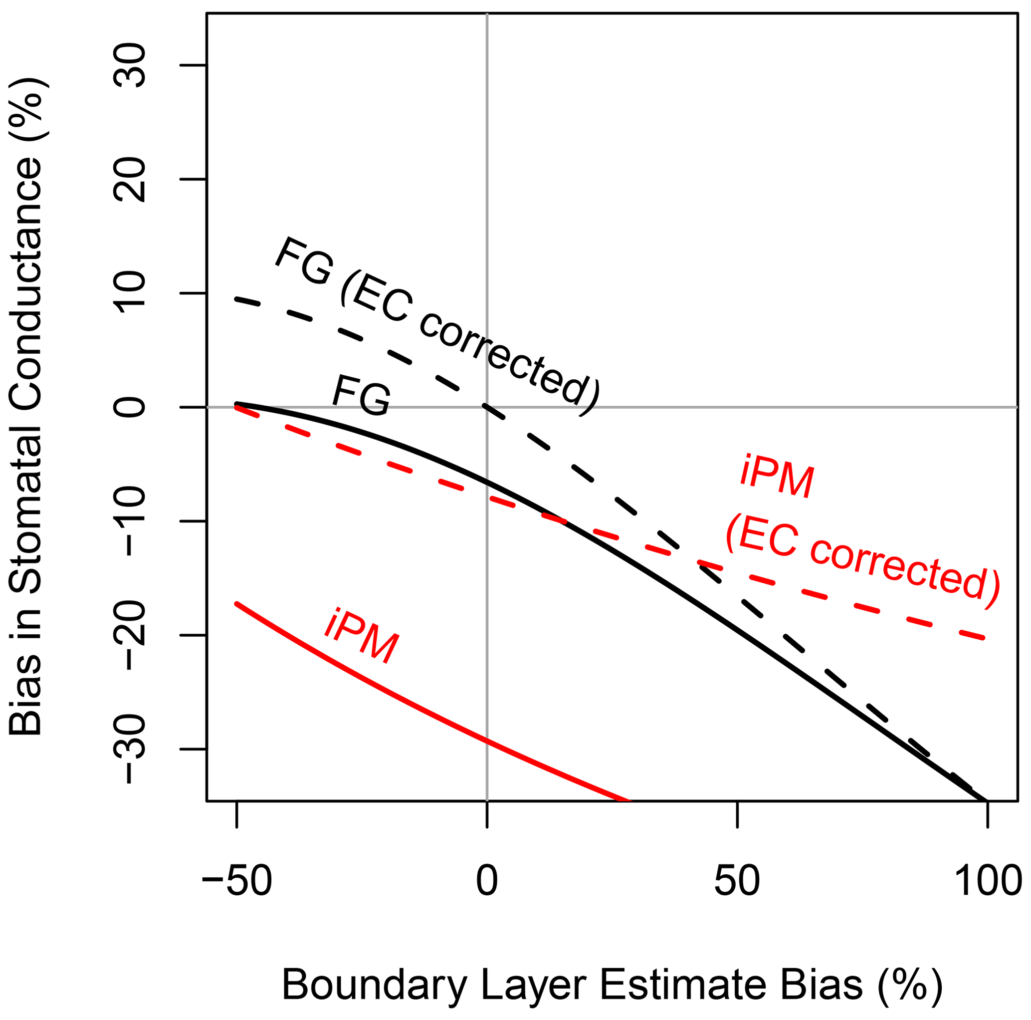
Figure 5Same as Fig. 4a, but with true boundary layer resistance increased to make the aerodynamic and stomatal conductances to water vapor equal, simulating very calm atmospheric conditions and increasing the sensitivity of the FG and iPM equations to the value used for the boundary layer resistance.
4.2 Relative biases over time in a real forest
Figure 6 compares the diurnal patterns of gsV calculated from real measurements at Howland Forest (Hollinger, 1996) using the FG (black) and iPM (red) formulations. Solid lines show results based on the original EC fluxes and dotted lines show results based on adjusted EC fluxes that closed the long-term energy budget while preserving the measured Bowen ratio (the same adjustment as shown in Fig. 3). As usual at EC sites, heat storage was not measured and was therefore omitted from the iPM equation. If the bias in A did indeed average out at the monthly timescale, and if the measured Bowen ratio and estimated aerodynamic resistances were accurate, then the true values of gsV in Fig. 6 should be those obtained using the FG formulation with adjusted EC fluxes (dotted black lines). That flux adjustment was relatively small at this site in the summer of 2014: the slope of hourly H+LE versus hourly Rn−G was only 0.63, while the slope using daily data was 0.92, suggesting that 78 % of the hourly energy budget gap was due to the omission of S and only 22 % was due to EC. Besides the expected negative bias in the iPM approach, Fig. 6 shows that the iPM and FG formulations claim noticeably different diurnal patterns for gsV. In particular, the iPM equation gives substantially lower values than the FG formulation through the morning and early afternoon but then converges on the FG formulation in the late afternoon. The diurnal curve obtained from the iPM equation is therefore too flat, leading to an understated picture of the response of gsV to the vapor pressure deficit (which peaks in the afternoon), and/or to an exaggerated picture of the saturation of gsV at high light. This time-varying discrepancy between the FG and iPM approaches can be explained by the fact that S (and therefore negative bias in the iPM equation) generally peaks in the late morning and approaches zero in the late afternoon (Grace et al., 1995; Lindroth et al., 2010), as reflected in the energy budget gap shown in the bottom panel of Fig. 6 (grey shading).
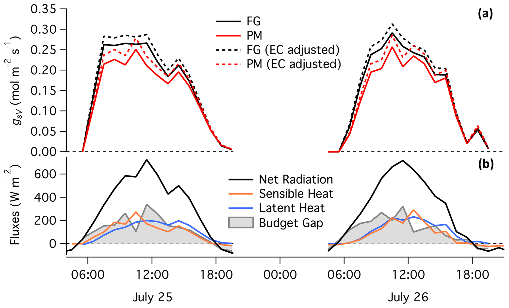
Figure 6(a) Hourly canopy stomatal conductance to water vapor calculated at Howland Forest (Hollinger, 1996) over 2 d in 2014 by the same approaches as in Fig. 3. (b) Measured energy fluxes and budget gap.
We have shown that for the purpose of determining canopy stomatal conductance at eddy covariance sites, the inverted Penman–Monteith equation is an inaccurate and unnecessary approximation to the flux–gradient equations for sensible heat and water vapor. Incomplete measurement of the energy budget at EC sites causes substantial bias and misleading spatial and temporal patterns in canopy stomatal conductance derived via the iPM equation, even after attempted eddy flux corrections. The biases in iPM stomatal conductance vary between 0 % and ∼ 30 % depending on the time of day and the site characteristics, resulting in erroneous relationships between stomatal conductance and driving variables such as light and vapor pressure deficit. Models trained on those relationships can be expected to misrepresent canopy carbon–water dynamics and to make incorrect predictions.
In theory, the FG equations are mathematically equivalent to the iPM equation aside from the relatively minor psychrometric approximation in the latter. In practice, however, errors in H and LE push gsV in opposite directions and so it is crucial that the FG equations receive underestimates of H and LE whereas the iPM equation implicitly overestimates from overestimates of A () and underestimates of LE. As a result, bias in gsV tends to be only about half as large in the FG equations as in the iPM equation. Moreover, if the eddy fluxes can be properly corrected, then the FG equations become unbiased while the iPM equation still suffers from bias in A.
Unfortunately, there does not appear to be a universally appropriate method for correcting the eddy fluxes at present. When the Bowen ratio is low or moderate in tall vegetation like forests, the published evidence supports increasing H and LE proportionally to close the long-term energy budget. However, when the Bowen ratio is high, the evidence suggests that H needs a disproportionally larger correction than LE. In that case, we have shown that a Bowen-ratio-preserving correction can make the bias in gsV worse.
Our results suggest that future studies should use the FG equations in place of the iPM equation and that published results based on the iPM equation may need to be revisited. It also motivates further work to determine a general and reliable framework for correcting the measured fluxes of sensible and latent heat at eddy covariance sites.
The canopy flux-weighted leaf boundary layer resistance to heat transfer from all sides of a leaf or needle (s m−1) can be estimated approximately as (McNaughton and Hurk, 1995; Wehr and Saleska, 2015)
where LAI is the single-sided leaf area index, L is the characteristic leaf (or needle cluster) dimension (e.g., 0.1 m), uh is the mean wind speed (m s−1) at the canopy top height h (m), ζ is height normalized by h, ϕ(ζ) is the vertical profile of the heat source (which can be approximated by the vertical profile of light absorption) normalized such that , and α is the extinction coefficient for the assumed exponential wind profile:
where . The wind speed at the top of the canopy can be obtained from Eq. (A2) with ζ set to correspond to the wind measurement height atop the flux tower.
The R code used for the simulations and the Igor Pro code used for the Howland Forest data analysis are freely available in the Dryad data archive under the digital object identifier https://doi.org/10.5061/dryad.h44j0zpgp (Wehr and Saleska, 2020).
RW conceived and designed the study, wrote the software code, performed the simulations, and prepared the manuscript with contributions from SRS.
The authors declare that they have no conflict of interest.
Funding for AmeriFlux data resources was provided by the U.S. Department of Energy's Office of Science. The Howland Forest data were produced under the supervision of David Hollinger.
This research has been supported by the National Science Foundation, Division of Environmental Biology (grant no. 1754803).
This paper was edited by Christopher Still and reviewed by Bharat Rastogi and one anonymous referee.
Baldocchi, D. D., Luxmoore, R. J., and Hatfield, J. L.: Discerning the forest from the trees: an essay on scaling canopy stomatal conductance, Agr. Forest Meteorol., 54, 197–226, 1991.
Charuchittipan, D., Babel, W., Mauder, M., Leps, J.-P., and Foken, T.: Extension of the Averaging Time in Eddy-Covariance Measurements and Its Effect on the Energy Balance Closure, Bound.-Lay. Meteorol., 152, 303–327, 2014.
Foken, T.: The energy balance closure problem: An overview, Ecol. Appl., 18, 1351–1367, 2008.
Franssen, H. J. H., Stöckli, R., Lehner, I., Rotenberg, E., and Seneviratne, S. I.: Energy balance closure of eddy-covariance data: A multisite analysis for European FLUXNET stations, Agr. Forest Meteorol., 150, 1553–1567, 2010.
Gatzsche, K., Babel, W., Falge, E., Pyles, R. D., Paw U, K. T., Raabe, A., and Foken, T.: Footprint-weighted tile approach for a spruce forest and a nearby patchy clearing using the ACASA model, Biogeosciences, 15, 2945–2960, https://doi.org/10.5194/bg-15-2945-2018, 2018.
Grace, J., Lloyd, J., and McIntyre, J.: Fluxes of carbon dioxide and water vapour over an undisturbed tropical forest in south-west Amazonia, Glob. Change Biol., 1, 1–12, 1995.
Hicks, B. B., Baldocchi, D. D., Meyers, T. P., Hosker Jr., R. P., and Matt, D. R.: A preliminary multiple resistance routine for deriving dry deposition velocities from measured quantities, Water Air Soil Poll., 36, 311–330, 1987.
Hollinger, D.: AmeriFlux US-Ho1 Howland Forest (main tower), dataset, https://doi.org/10.17190/AMF/1246061, 1996.
Jarvis, P. G. and McNaughton, K. G.: Stomatal Control of Transpiration: Scaling Up from Leaf to Region, Adv. Ecol. Res., 15, 1–49, 1986.
Leuning, R., Cleugh, H. A., Zegelin, S. J., and Hughes, D.: Carbon and water fluxes over a temperate Eucalyptus forest and a tropical wet/dry savanna in Australia: measurements and comparison with MODIS remote sensing estimates, Agr. Forest Meteorol., 129, 151–173, 2005.
Leuning, R., van Gorsel, E., Massman, W. J., and Isaac, P. R.: Reflections on the surface energy imbalance problem, Agr. Forest Meteorol., 156, 65–74, 2012.
Lindroth, A., Mölder, M., and Lagergren, F.: Heat storage in forest biomass improves energy balance closure, Biogeosciences, 7, 301–313, https://doi.org/10.5194/bg-7-301-2010, 2010.
Mauder, M., Foken, T., and Cuxart, J.: Surface-Energy-Balance Closure over Land: A Review, Bound.-Lay. Meteorol., 177, 395–426, https://doi.org/10.1007/s10546-020-00529-6, 2020.
McColl, K. A.: Practical and Theoretical Benefits of an Alternative to the Penman-Monteith Evapotranspiration Equation, Water Resour. Res., 56, 205–215, 2020.
McNaughton, K. G. and Hurk, B. A.: `Lagrangian' revision of the resistors in the two-layer model for calculating the energy budget of a plant canopy, Bound.-Lay. Meteorol., 74, 261–288, 1995.
Monteith, J.: Evaporation and environment, Symp. Soc. Exp. Biol., 19, 205–234, 1965.
Purdy, A. J., Fisher, J. B., Goulden, M. L., and Famiglietti, J. S.: Ground heat flux: An analytical review of 6 models evaluated at 88 sites and globally, J. Geophys. Res.-Biogeosci., 121, 3045–3059, 2016.
Reed, D. E., Frank, J. M., Ewers, B. E., and Desai, A. R.: Time dependency of eddy covariance site energy balance, Agr. Forest Meteorol. 249, 467–478, 2018.
Schymanski, S. J. and Or, D.: Leaf-scale experiments reveal an important omission in the Penman–Monteith equation, Hydrol. Earth Syst. Sci., 21, 685–706, https://doi.org/10.5194/hess-21-685-2017, 2017.
Stoy, P. C., Mauderb, M., Foken, T., Marcolla, B., Boegh, E., Ibrom, A., Arain, M. A., Arneth, A., Aurela, M., Bernhofer, C., Cescatti, A., Dellwik, E., Duce, P., Gianelle, D., van Gorsel, E., Kiely, G., Knohl, A., Margolis, H., McCaughey, H., Merbold. L., Montagnani, L., Papale, D., Reichstein, M., Saunders, M., Serrano-Ortiz, P., Sottocornola, M., Spano D., Vaccari, F., and Varlagin, A.: A data-driven analysis of energy balance closure across FLUXNET research sites: The role of landscape scale heterogeneity, Agr. Forest Meteorol., 171–172, 137–152, 2013.
Twine, T. E., Kustas, W. P., Norman, J. M., Cook, D. R., Houser, P. R., Meyers, T. P., Prueger, J. H., Starks, P. J., and Wesely, M. L.: Correcting eddy-covariance flux underestimates over a grassland, Agr. Forest Meteorol., 103, 279–300, 2000.
Wehr, R. and Saleska, S. R.: An improved isotopic method for partitioning net ecosystem–atmosphere CO2 exchange, Agr. Forest Meteorol., 214–215, 515–531, 2015.
Wehr, R., Commane, R., Munger, J. W., McManus, J. B., Nelson, D. D., Zahniser, M. S., Saleska, S. R., and Wofsy, S. C.: Dynamics of canopy stomatal conductance, transpiration, and evaporation in a temperate deciduous forest, validated by carbonyl sulfide uptake, Biogeosciences, 14, 389–401, https://doi.org/10.5194/bg-14-389-2017, 2017.
Wehr, R. and Saleska, S.: Software code for simulations and analyses concerning the calculation of canopy stomatal conductance at eddy covariance sites, Dryad, Dataset, https://doi.org/10.5061/dryad.h44j0zpgp, 2020.
Wilson, K., Goldstein, A., Falge, E., Aubinet, M., Baldocchi, D., Berbigier, P., Bernhofer, C., Ceulemans, R., Dolman, H., Field, C., Grelle, A., Ibrom, A., Law, B.E., Kowalski, A., Meyers, T., Moncrieff, J., Monson, R., Oechel, W., Tenhunen, J., Valentini, R., and Verma, S.: Energy balance closure at FLUXNET sites, Agr. Forest Meteorol., 113, 223–243, 2002.
Wohlfahrt, G., Haslwanter, A., Hörtnagl, L., Jasoni, R. L., Fenstermaker, L. F., Arnone III, J. A., and Hammerle, A.: On the consequences of the energy imbalance for calculating surface conductance to water vapour, Agr. Forest Meteorol., 149, 1556–1559, 2009.
World Meteorological Organization: Guide to Meteorological Instruments and Methods of Observation No. WMO-No. 8, 2008.