Plant phenology evaluation of CRESCENDO land surface models – Part 1: Start and end of the growing season

Plant phenology plays a fundamental role in land–atmosphere interactions, and its variability and variations are an indicator of climate and environmental changes. For this reason, current land surface models include phenology parameterizations and related biophysical and biogeochemical processes. In this work, the climatology of the beginning and end of the growing season, simulated by the land component of seven state-of-the-art European Earth system models participating in the CMIP6, is evaluated globally against satellite observations. The assessment is performed using the vegetation metric leaf area index and a recently developed approach, named four growing season types. On average, the land surface models show a 0.6-month delay in the growing season start, while they are about 0.5 months earlier in the growing season end. The difference with observation tends to be higher in the Southern Hemisphere compared to the Northern Hemisphere. High agreement between land surface models and observations is exhibited in areas dominated by broadleaf deciduous trees, while high variability is noted in regions dominated by broadleaf deciduous shrubs. Generally, the timing of the growing season end is accurately simulated in about 25 % of global land grid points versus 16 % in the timing of growing season start. The refinement of phenology parameterization can lead to better representation of vegetation-related energy, water, and carbon cycles in land surface models, but plant phenology is also affected by plant physiology and soil hydrology processes. Consequently, phenology representation and, in general, vegetation modelling is a complex task, which still needs further improvement, evaluation, and multi-model comparison.

1 Introduction

Plant phenology and its variability have a substantial influence on the terrestrial ecosystem (e.g. Churkina et al., 2005; Kucharik et al., 2006; Berdanier and Klein, 2011) and land–atmosphere interactions (e.g. Cleland et al., 2007; Richardson et al., 2013; Keenan et al., 2014). Moreover, recent decades observations show modifications in both spring and autumn phenology under global warming (e.g. Menzel et al., 2006; Richardson et al., 2013; Park et al., 2016; Zhu et al., 2016; Chen et al., 2020; Zhang et al., 2020). For these reasons, phenology variability is one of the indicators of climate change (e.g. Schwartz et al., 2006; Soudani et al., 2008; Jeong et al., 2011).

Given the influence of plant phenology on vegetation productivity, and since green leaves are the primary interface for the exchange of energy, mass (e.g. water, nutrient, and CO₂), and momentum between the terrestrial surface and the planetary boundary layer (Richardson et al., 2012), land surface models (LSMs) need to accurately simulate plant growing season cycles. Limitations may result in biases and uncertainties in representing the vegetation productivity and carbon cycle (e.g. Churkina et al., 2005; Kucharik et al., 2006; Berdanier and Klein, 2011; Richardson et al., 2012; Friedlingstein et al., 2014; Savoy and Mackay, 2015; Buermann et al., 2018). For example, Kucharik et al. (2006) show an overestimated April–May net ecosystem production triggered by biases in plant budburst. Berdanier and Klein (2011) describe a link between above-ground net primary production, growing season length, and soil moisture in high-elevation meadows. They show that the potential impact of changes in active growing season length on biomass production accounts for about 3–4 g m⁻² d⁻¹. The work by Richardson et al. (2012) is an example of a systematic evaluation of LSMs' phenology representation. They evaluate 14 models participating in the North American Carbon Program Site Synthesis against 10 forested sites, within the AmeriFlux and FLUXNET Canada networks. Their assessment reveals a typical bias of about 2 weeks in LSM representation of the beginning and end of the growing season. They also show a low skill in LSMs' reproduction of the observed inter-annual phenology variability. These biases lead to an overestimation of about 235 gC m⁻² yr⁻¹ in the gross ecosystem photosynthesis of deciduous forest sites. However, uncertainties in simulated maximum production partially balance this overestimation. The work by Buermann et al. (2018) is another example of a multi-LSM evaluation. They observe widespread lagged plant productivity responses across northern ecosystems associated with warmer and earlier springs, which is weakly captured by 10 evaluated TRENDYv6 current LSMs. Consequently, current LSMs still present biases in simulating timings and the magnitude of the vegetation active season.

The latest generation of LSMs have started including a more detailed description of land biophysical and biogeochemical processes, and they have become able to explicitly represent carbon and nitrogen land cycles, as well as plant phenology and related water and energy cycling on a global scale (e.g. Oleson et al., 2013; Lawrence et al., 2018). In particular, current LSMs link leaf area index (LAI) and plant phenology to changes in temperature, precipitation, soil moisture, and light availability (e.g. Oleson et al., 2013; Lawrence et al., 2018), as displayed in observations (e.g. Caldararu et al., 2012; Zeng et al., 2013; Tang and Dubayah, 2017). Besides, some LSMs use satellite‐based data assimilation as a tool to constrain the parameters of phenology schemes (e.g. Knorr et al., 2010; Stöckli et al., 2011; MacBean et al., 2015).

In this framework, the European CRESCENDO project (https://www.crescendoproject.eu/, last access: 7 June 2020) fostered the development of a new generation of LSMs to be used as the land component of the Earth system models (e.g. Smith et al., 2014; Olin et al., 2015; Cherchi et al., 2019; Mauritsen et al., 2019; Sellar et al., 2020; Seland et al., 2020; Yool et al., 2020; Boucher et al., 2020) employed in the Coupled Model Intercomparison Project Phase 6 (CMIP6, Eyring et al., 2016). In particular, seven novel LSMs, which are part of the CRESCENDO effort, are used in this work, namely the Community Land Model (CLM) version 4.5 (Oleson et al., 2013) and version 5.0 (Lawrence et al., 2019), JULES-ES (Wiltshire et al., 2020a), JSBACH (Mauritsen et al., 2019), LPJ-GUESS (Lindeskog et al., 2013; Smith et al., 2014; Olin et al., 2015), ORCHIDEE (Krinner et al., 2005), and ISBA-CTRIP (Decharme et al., 2019).

Given the relevance of plant phenology and its changing variability related to climate, LSMs need routine evaluation against observations (e.g. Jolly et al., 2005; Richardson et al., 2012; Dalmonech and Zaehle, 2013; Kelley et al., 2013; Murray-Tortarolo et al., 2013; Anav et al., 2013; Forkel et al., 2015; Peano et al., 2019). This study aims to evaluate the ability and limits of the novel CRESCENDO LSMs to represent the global climatology of the start and end of growing season timings. The CRESCENDO LSMs cover a wide range of phenology schemes and vegetation descriptions. This selection may therefore help understand the sources of differences between LSMs' representation of phenology and the regions where plant phenology simulations remain difficult.

Vegetation phenology can be assessed by considering different plant features and indices, such as leaf colour (e.g. normalized difference vegetation index, NDVI, Churkina et al., 2005; Keenan et al., 2014), the fraction of absorbed photosynthetically active radiation (e.g. Kelley et al., 2013; Forkel et al., 2015), or canopy density (e.g. LAI, Murray-Tortarolo et al., 2013; Peano et al., 2019). Each methodology presents skills and limitations (e.g Forkel et al., 2015). In this work, the novel four growing season types (4GST) methodology developed by Peano et al. (2019) is used to evaluate phenology. This method proved good skill in capturing the principal global phenology cycles (Peano et al., 2019) and integrates a broader spectrum of growing season modes compared to previous techniques (e.g. Murray-Tortarolo et al., 2013). The set of growing season modes investigated in 4GST are (1) evergreen phenology, (2) single growing season with summer LAI peak, (3) single growing season with summer dormancy, and (4) two growing seasons. 4GST uses LAI data to evaluate phenology. Most ecosystem and climate models introduce leaf area as a fundamental state parameter describing the interactions between the biosphere and the atmosphere. The most common measure of the area of leaves is the LAI, which is generally defined as the one-sided leaf surface area divided by the ground area in m² m⁻² (Chen and Black, 1992). In addition, LAI is the key variable by which LSMs scale up leaf-level processes to canopy and ecosystem scale exchanges of carbon, energy, and water. This makes the LAI a reasonable choice for the evaluation of the LSMs' phenology (Murray-Tortarolo et al., 2013; Peano et al., 2019).

In this paper, we present a brief description of the methods, LSMs, and satellite data used (Sect. 2). Next, we present the main results of the satellite data comparison and evaluation of LSMs against observations (Sect. 3). Finally, we discuss the methodology, data, and results (Sect. 4), followed by concluding remarks (Sect. 5).

2 Method, models, and data

2.1 Satellite observation

To perform a comprehensive global phenology evaluation, a satellite-based observational dataset is required. LAI satellite observations present uncertainties and limitations related to the assumptions and algorithms applied in the LAI calculation (Sect. 4.2, e.g. Fang et al., 2013; Forkel et al., 2015; Jiang et al., 2017). For this reason, three different satellite observational products are considered in this work.

1. The full time series of LAI3g data is generated by an artificial neural network (ANN) algorithm that is trained with the overlapping data of the third-generation Global Inventory Modeling and Mapping Studies (GIMMS) NDVI3g and Terra Moderate Resolution Imaging Spectroradiometer (MODIS) LAI products (see Zhu et al., 2013). It covers the 1982–2011 period with a 15 d temporal frequency and a $\mathrm{1}/\mathrm{12}$^∘ spatial resolution.

2. The MODIS (MOD15A2H and MYD15A2H version 6, https://lpdaac.usgs.gov/, last access: 13 November 2019; Myneni et al., 2015a, b) LAI algorithm is based on a three-dimensional radiative transfer equation that links surface spectral bidirectional reflectance factors to vegetation canopy structural parameters (see Yan et al., 2016a). It covers the 2000–2017 period with a 4 or 8 d temporal frequency and a 500 m spatial resolution.

3. The Copernicus Global Land Service (CGLS, LAI 1 km version 2, https://land.copernicus.eu/global/products/LAI, last access: 11 March 2020; Maisongrande et al., 2004; Drusch et al., 2012) LAI dataset is obtained through a neural network applied on top-of-atmosphere input reflectances in red and near-infrared bands derived from SPOT and PROBA-V. The instantaneous LAI estimates obtained in this way go through a temporal smoothing and small gap filling, which discriminate between evergreen broadleaf forest and no-evergreen broadleaf forest pixels (see Verger et al., 2019, 2011). It covers the 1999–2019 period with a 10 d temporal frequency and a 1 km spatial resolution. Note that CGLS has a reduced latitudinal coverage compared to MODIS and LAI3g since it covers up to 75^∘ N versus the 90^∘ N of the other two products.

The 2000–2011 period is common to the three satellite datasets, and it is used in the present analysis. The satellite observations are aggregated into monthly values and regridded, by means of a first-order conservative remapping scheme (Jones, 1999), to a regular 0.5^∘ × 0.5^∘ grid for consistency with the LSMs' output. The regridding operation is directly applied to the gap-filled satellite data. Note that regridding does not employ any specific treatment for differences in land cover.

To perform biome-level analysis, the observed ESA CCI land cover map (https://www.esa-landcover-cci.org/, last access: 10 December 2019) has been used to define a standard regional vegetation distribution. In particular, Li et al. (2018) aggregated the original 37 ESA CCI land cover classes into 0.5^∘ spatial resolution and translated them into 14 plant functional types (PFTs) based on an adjusted cross-walking table. These data have been used to obtain an observed dominant PFT map for the 2000–2011 period. Based on Li et al. (2018), all vegetation types are classified into 10 categories: broadleaf evergreen tree (BET), broadleaf deciduous tree (BDT), needle-leaf evergreen tree (NET), needle-leaf deciduous tree (NDT), broadleaf evergreen shrub (BES), broadleaf deciduous shrub (BDS), needle-leaf evergreen shrub (NES), needle-leaf deciduous shrub (NDS), grass-covered areas (Grass), and crop-covered areas (Crop).

2.2 Land surface models

Seven European LSMs, which are part of the CRESCENDO project, are evaluated in this study. Further details on each of these LSMs are provided in the following sections and briefly summarized in Table 1.

Zeng (2001)Jackson et al. (1996)Wiltshire et al. (2020a)Kleidon (2004)Krinner et al. (2005)Canadell et al. (1996)Oleson et al. (2013)Lawrence et al. (2018)Clark et al. (2011)Mauritsen et al. (2019)Reick et al. (2021)Smith et al. (2014)Botta et al. (2000)Krinner et al. (2005)Delire et al. (2020)

Table 1 (a) Grid spatial resolution used for each land surface model (LSM) and brief summary of their main features. PFT stands for plant functional type and CFT stands for crop functional type. Part (b) gives further details on the temperature and moisture thresholds for the start (S) and end (E) of the growing season in the phenology schemes.

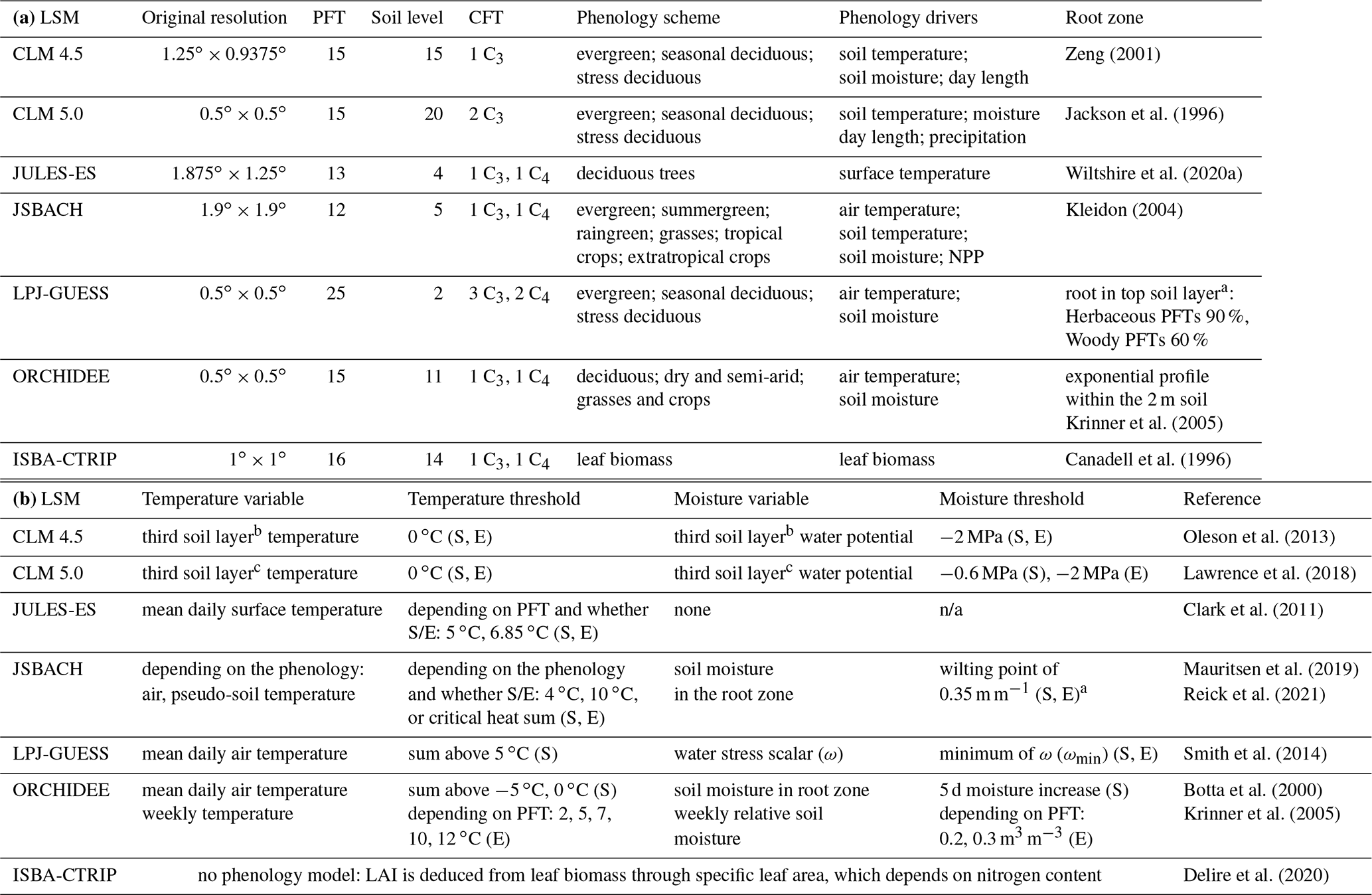
^a Relative soil moisture content above which growth is possible and below which growth stops and shedding sets in. ^b About 6 cm depth. ^c 9 cm depth. n/a – not applicable.

2.2.1 Community Land Model version 4.5

The Community Land Model (CLM) is the terrestrial component of the Community Earth System Model version 1.2 (CESM1.2, http://www.cesm.ucar.edu/models/cesm1.2/, last access: 1 June 2019). In its version 4.5 (CLM4.5,  Oleson et al., 2013) and biogeochemical configuration (i.e. BGC compset, Koven et al., 2013), it is the land component of the CMCC coupled model version 2 (CMCC-CM2, Cherchi et al., 2019). CLM4.5-BGC features 15 PFTs, in which crop is represented as a generic C₃ crop. The PFTs time evolution follows the area changes described in the Land Use Harmonization version 2 dataset (LUH2, Hurtt et al., 2020). CLM4.5-BGC resolves explicitly plant phenology (Oleson et al., 2013; Koven et al., 2013), which is described by means of three specific parameterizations: (1) evergreen plant phenology, (2) seasonal-deciduous plant phenology, and (3) stress-deciduous plant phenology (Oleson et al., 2013).

The CLM4.5 representation of phenology is based on soil temperature, soil moisture, and day length. In particular, the leaf onset in the seasonal-deciduous plant phenology starts when the soil temperature of accumulated growing degree day (GDD) passes a critical threshold. The leaf litterfall, instead, starts when the day length exceeds another specific threshold (Oleson et al., 2013). In the stress-deciduous plant phenology, soil moisture and soil temperature drive the start and end of the growing season. For example, the leaf onset is soil-moisture-driven in areas characterized by year-round warm conditions. Finally, the evergreen plant phenology is characterized by a background litterfall, which is a continuous leaf fall and fine root turnover distributed throughout the year. A PFT-specific leaf longevity parameter drives this mechanism. Further details can be found in Oleson et al. (2013).

2.2.2 Community Land Model version 5.0

CLM version 5.0 (CLM5.0) is the terrestrial component of the Community Earth System Model version 2 (CESM2, http://www.cesm.ucar.edu/models/cesm2/) and of the Norwegian Earth System Model version 2 (NorESM2,  Seland et al., 2020).

CLM5.0 uses the same number of default PFTs, while the crop module uses two C₃ crop configurations: C₃ rainfed and C₃ irrigated. The irrigation area is based on crop type and region, and the irrigation triggers for crop phenology are newly updated from the CLM4.5.

CLM5.0 uses the same three specific plant phenology parameterizations applied in CLM4.5 (Lawrence et al., 2018). Differently from CLM4.5, CLM5.0 includes also precipitation in the stress-deciduous phenology scheme. In particular, antecedent rain is required to start leaf onset; this is done to reduce the occurrence of anomalous green-up during the dry season driven by upwards water movement from wet to dry soil layers (Dahlin et al., 2015).

Several major changes have been made in CLM5.0. One of the physiological changes includes maximum stomatal conductance, which now uses the Medlyn conductance model (Medlyn et al., 2011) rather than the previously used Ball–Berry stomatal conductance model. In CLM5.0, the Jackson et al. (1996) rooting profiles are used for both water and carbon, where the rooting depths were increased for broadleaf evergreen and broadleaf deciduous tropical tree PFTs. These features impact on soil moisture and plant hydrology that control stress-deciduous plant phenology. Other modifications that might influence phenology include nutrient dynamics, hydrological and snow parameterizations, plant hydraulic functions, revised nitrogen cycling with flexible leaf stoichiometry, leaf N optimization for photosynthesis, and carbon costs for plant nitrogen uptake (Lawrence et al., 2019).

2.2.3 JULES-ES

JULES-ES is the Earth System configuration of the Joint UK Land Environment Simulator (JULES). JULES-ES is the terrestrial component of the new UK community ESM, UKESM1 (Sellar et al., 2020). It is based on the core physical land configuration of JULES (JULES-GL7) as described in Wiltshire et al. (2020a). The simulations described here used a near-final configuration of JULES-ES prior to the final tuning performed as part of UKESM1 (Yool et al., 2020). JULES-ES is run offline forced by global historic meteorological data as described in Sect. 2.3.

JULES-ES includes a full carbon and nitrogen cycle with dynamic vegetation (Wiltshire et al., 2020b), 13 plant functional types with trait-based physiology (Harper et al., 2016), and a representation of crop harvest and land-use change. In JULES-ES, the allometrically defined maximum LAI varies with the carbon status (Clark et al., 2011) and extent of the underlying vegetation. In the case of natural grasses, maximum LAI can vary rapidly sub-seasonally, whereas tree PFTs have a smaller variation. Phenology operates on top of this variation for deciduous broadleaf and needle-leaf PFTs based on an accumulated thermal time model. Consequently, JULES-ES features one phenology scheme, which relies on thermal conditions.

2.2.4 JSBACH

JSBACH3.2 is the land component of MPI-ESM1.2 (Mauritsen et al., 2019). For the simulations described here, JSBACH3.2 is run offline at T63 (∼ 1.9^∘) resolution. Simulations were conducted without natural changes in the land cover; instead, a static map of natural land cover based on Pongratz et al. (2008) was used. Anthropogenic land cover changes were applied using land-use transitions (see  Reick et al., 2013) derived from the LUH2 forcing, whereby rangelands were treated as natural vegetation (see also  Mauritsen et al., 2019). Simulations were conducted according to the common CRESCENDO protocol as described in Sect. 2.3, with the only difference being that land-use change was already simulated starting at 1700 to avoid a cold start problem when applying land-use transitions. JSBACH3.2 contains a multilayer hydrology model (Hagemann and Stacke, 2015) and a representation of the terrestrial nitrogen cycle (Goll et al., 2017).

JSBACH3.2 is run with its default phenology model, called LoGro-P, as evaluated in Böttcher et al. (2016) and Dalmonech et al. (2015). This phenology is based on a logistic equation for the temporal development of the LAI. Under ideal environmental conditions, the LAI approaches a maximum value representing a prescribed PFT-specific physiological limit. Growth and leaf shedding rates of the logistic equation are functions of environmental conditions, chosen differently according to the phenology type (see e.g. Böttcher et al., 2016). JSBACH3.2 distinguishes the following phenology types: (1) evergreen, (2) summergreen, (3) raingreen, (4) grasses, and (5) tropical and extratropical crops.

In general, JSBACH3.2 features a higher amount of phenology schemes (i.e. five) compared to the other LSMs, which are driven by soil temperature, air temperature, soil moisture, and net primary productivity (NPP). In particular, the phase changes in evergreen and summergreen phenologies are determined by temperature thresholds calculated by the alternating model of Murray et al. (1989) from heat sums, chill days, and critical soil temperatures. The raingreen phenology has a non-zero growth rate whenever the soil moisture exceeds the wilting point and the NPP is positive. The shedding rate depends on the relative soil water content. The grass phenology resembles the raingreen phenology but further requires the air temperature and soil moisture to exceed a critical value for a non-zero growth rate. Because grass roots are less deep than tree roots, the soil moisture is taken from the upper soil layer for the grass phenology. The crop phenology is modelled as a function of NPP and distinguishes tropical and extratropical crops in order to reflect different farming practices in dependence of the prevailing climatic conditions. The vegetation in the conducted JSBACH3.2 simulations was represented by 12 PFTs, each of which is linked to one of the phenology types: one forest type with evergreen phenology, one forest and one shrub type with summergreen phenology, two forest types and one shrub type with raingreen phenology, C₃ and C₄ grasses as well as C₃ and C₄ pastures with grass phenology, and C₃ and C₄ crops with extratropical and tropical crop phenology, respectively.

2.2.5 LPJ-GUESS

The Lund–Potsdam–Jena General Ecosystem Simulator version 4.0 (LPJ-GUESS;  Lindeskog et al., 2013; Smith et al., 2014; Olin et al., 2015), a process-based second-generation dynamic vegetation and biogeochemistry model, is the terrestrial biosphere component used in the European community Earth-System Model (EC-Earth-Veg, http://www.ec-earth.org/, last access: 1 June 2019; Hazeleger and Bintanja, 2012; Döscher et al., 2021; Miller et al., 2021). It simulates vegetation dynamics, land use, and land management following LUH2 (Hurtt et al., 2020). LPJ-GUESS features 25 PFTs, and 10 woody and 2 herbaceous PFTs compete in the natural stand fractions, whereas two herbaceous species, C₃ and C₄ photosynthesis pathways, compete in pasture, urban, and peatland fractions. Crop stands have each five crop functional types representing the properties of global crop types and correspond to the classes found in LUH2, namely both annual and perennial C₃ and C₄ crops, and C₃ N fixers, and two herbaceous cover crops (C₃ and C₄) that are grown in between the main agricultural growing seasons.

Similar to CLM4.5 and CLM5.0, LPJ-GUESS plant phenology is described by means of three specific parameterizations: (1) evergreen plant phenology, (2) seasonal-deciduous plant phenology, and (3) stress-deciduous plant phenology (Smith et al., 2014). An explicit phenological cycle is simulated only for leaves and fine roots in seasonal-deciduous and stress-deciduous PFTs, whereas evergreen PFTs have a prescribed background litterfall for leaves, fine roots, and sapwood. Seasonal-deciduous plant phenology is based on a PFT-dependent accumulated GDD sum threshold for leaf onset, with leaf area rising from 0 to the pre-determined annual maximum leaf area linearly with an additional 200 (100 for herbaceous and needle-leaved tree PFTs) degree days above a threshold of 5 ^∘C. For seasonal-deciduous PFTs, growing season length is fixed, with all leaves being shed after the equivalent of 210 d with full leaf cover. Stress-deciduous plant phenology PFTs shed their leaves whenever the water stress scalar ω drops below a threshold, ω_min, signifying the onset of a drought period or dry season. New leaves are produced after a prescribed minimum dormancy period, when ω again rises above ω_min (Smith et al., 2014). Crop PFT sowing and harvest decisions are modelled based on climate variability (Waha et al., 2011; Lindeskog et al., 2013) and climatic thresholds (Bondeau et al., 2007).

2.2.6 ORCHIDEE

The ORCHIDEE model used for the CRESCENDO simulations is the land component of the IPSL (Institut Pierre Simon Laplace) ESM used for the CMIP6 simulations (Boucher et al., 2020). The surface heterogeneity is described with 15 different PFTs that can be mixed in each grid cell. The annual evolution of the PFT distribution is derived from the LUH2 database as described in more detail in Lurton et al. (2019). In each grid cell, the PFTs are grouped into three soil tiles according to their physiological behaviour: high vegetation (forests) with eight PFTs, low vegetation (grasses and crops) with six PFTs, and bare soil with one PFT. An independent hydrological budget is calculated for each soil tile to prevent forests from exhausting all soil moisture. In contrast, only one energy budget (and snow budget) is calculated for the whole grid cell. Note that since its first description in Krinner et al. (2005), the model has substantially evolved; we describe below only the main features relevant for this study.

A Phenology module describes leaf onset and leaf senescence for deciduous PFTs based on temperature and soil moisture. In temperate and boreal regions, leaf onset is driven by an accumulation of warm temperature in spring, following the concept of GDD. In addition, a minimum period of cold temperature, based on a number of chilling days (NCD), is used to avoid buds dying with late frosts. Both criteria are combined, with PFT-specific GDD and NCD thresholds to be met before leaves can start growing (see Botta et al., 2000 for more details). For the dry tropics and semi-arid ecosystems, a moisture availability criterion is used based on water accumulated in the soil. A minimum of 5 consecutive days with soil moisture increase (root zone) should occur after 1 January for the Northern Hemisphere and 1 July for the Southern Hemisphere, with the addition of a filter for small rises in soil moisture (see model 4b in Botta et al., 2000). Both temperature and moisture criteria are combined for grasses and crops, and the different parameters of the leaf onset parameterization have been calibrated with satellite data (Botta et al., 2000). Leaves are then further separated into four age classes with different photosynthetic efficiency. Leaf fall is controlled by different turnover processes. The first one is a simple ageing process, and a second senescence process based on climatic conditions (either based on air temperature or soil moisture conditions) is applied.

2.2.7 ISBA-CTRIP

ISBA-CTRIP is the land surface model of CNRM-ESM2-1 (http://www.umr-cnrm.fr/spip.php?article1092, last access: 1 June 2019). It is used within the SURFEX version 8 modelling platform representing surface exchanges between ocean, lakes, and land. It solves the energy, carbon, and water budgets at the land surface and was recently thoroughly upgraded (Decharme et al., 2019). The model distinguishes 16 vegetation types (nine tree, one shrub, three grass, and three crop types) alongside desert, rocks, and permanent snow. Decharme et al. (2019) give a detailed description of the physical aspects of the model.

Differently from the other LSMs, leaf phenology results directly from the daily carbon balance of the leaves. Leaf turnover time is dependent on potential leaf longevity reduced when 10 d assimilation rates start to decrease. Leaf area index is diagnosed from leaf biomass and specific leaf area index, which varies as a function of leaf nitrogen concentration and plant functional type. To allow for leaf growth after dormancy there is an imposed minimum leaf biomass. Crops have the same phenology as grasses. A detailed description of the terrestrial carbon cycle can be found in Delire et al. (2020).

2.3 Experimental setup

In this study, the S3 CRESCENDO simulations were used, characterized by transient CO₂, climate, and land-use forcing. Each model spin-up is obtained by recycling climate mean and variability from the period 1901–1920 with the pre-industrial (1860) atmospheric CO₂ concentration until carbon pools and fluxes reach a steady state. The 1861–1900 period is simulated using the same climate forcing as the spin-up, but with time-varying atmospheric CO₂ and land-use forcing. Finally, the LSMs are forced over the 1901–2014 period with changing CO₂, climate, and land-use forcing. All LSMs are commonly driven by the atmospheric forcing reanalysis CRUNCEP version 7 (Viovy, 2018), and the land-use data are taken from the Land Use Harmonization version 2 dataset (Hurtt et al., 2020). Note that the use of LUH2 land cover transitions differs across the models (see model description). CRUNCEPv7 provides for 2 m air temperature, precipitation, wind, surface pressure, shortwave radiation, long-wave radiation, and air humidity.

Each LSM is run on different spatial resolutions (Table 1), but the outputs of these simulations are provided on a regular 0.5^∘ × 0.5^∘ grid, over which simulations and observations are compared. CLM4.5, JULES-ES, JSBACH, and ISBA-CTRIP perform their simulations at a coarser resolution. Their output is regridded by applying a first-order conservative remapping method (Jones, 1999). The LAI monthly mean output from these simulations is used in the present analysis.

2.4 Growing season analysis

The times of the start and end of the growing season (GSS and GSE, respectively) are evaluated using the four growing season types (4GST) method introduced by Peano et al. (2019). The 4GST method has been shown to adequately capture the main global phenology cycles for evaluation of LSMs.

The 4GST method allows us to evaluate the start and end of the growing season and the global spatial distribution of four main growing season types: (1) evergreen (EVG), (2) single growing season peaking in summer (SGS-S), (3) single growing season with summer dormancy (SGS-D), and (4) two growing seasons (TGS). The EVG type is identified when relative changes in LAI annual cycle are smaller than 25 % of local LAI mean value. Note that GSS and GSE timings are not detected in EVG areas. The other three types are identified based on LAI slopes and transition timings as illustrated and summarized in Fig. 1. When one single growing season is identified, SGS-S and SGS-D are discerned based on the peak month (i.e. in the Northern Hemisphere (NH), SGS-S is detected when the LAI peak occurs between April and September – otherwise, SGS-D is detected; the opposite occurs in the Southern Hemisphere (SH): SGS-D is detected when the LAI peak occurs between April and September, and SGS-S is identified when LAI peaks in the other months). The timings of the start and end of the growing season are identified through a critical threshold set to 20 % of the annual LAI cycle (Fig. 1). TGS, instead, is identified when two growing seasons at least 3 months long are detected, and GSS and GSE timings are identified for each cycle. Further details can be found in Peano et al. (2019). Note that in this analysis the timings of the TGS GSS correspond to the GSS timings of the first growing season cycle, while the GSE timings are the second GSE timings, as described in Peano et al. (2019). The 4GST method is applied on monthly LAI data in this work, instead of the 15 d timescale used in Peano et al. (2019).

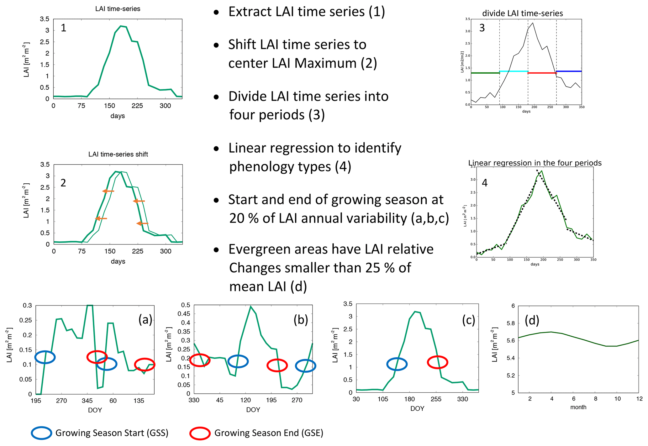
Figure 1 Scheme of the four growing season types method used in evaluating the start and end of the growing season.

3 Results

3.1 Satellite data comparison

We inspect the main differences between LAI3g, MODIS, and CGLS by plotting the spatial distribution of the four growing season types, GSS, and GSE (Fig. 2).

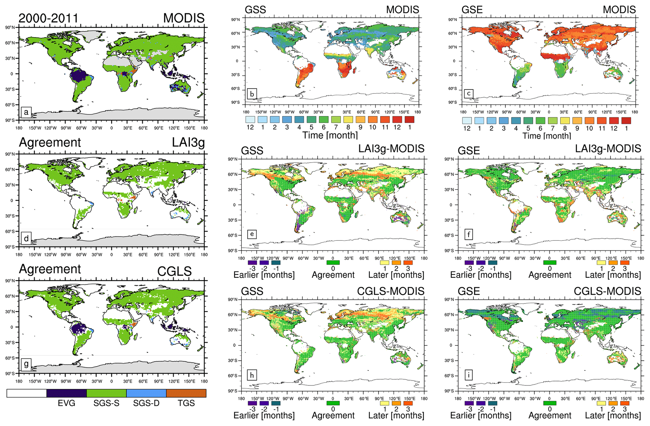
Figure 2 Global climatological (averaged over 2000–2011) distribution of (a) the four main growing season modes, (b) growing season start (GSS) timings, and (c) growing season end (GSE) timings for MODIS version 6. The other panels show the comparison between MODIS and LAI3g (second row) and CGLS (third row). In particular, panels (d) and (g) show the areas characterized by the same phenology types (d) between MODIS and LAI3g and (g) between MODIS and CGLS; panels (e) and (h) exhibit the difference in GSS timings; and panels (f) and (i) display the differences in GSE timings. In panels (d) and (g) white areas represent non-vegetated areas and regions of disagreement (d) between MODIS and LAI3g and (g) between MODIS and CGLS. White areas in panel (b), (c), (e), (f), (h), and (i) show evergreen and non-vegetated areas.

The three products show a high consistency in the distribution of growing season types (agreement of about 80 %, Table 2), with the main differences occurring in tropical regions, such as in the Amazon and Congo basins, and in semi-arid areas, such as central Australia (Fig. 2a, d, g). Compared to MODIS, LAI3g differs mainly in EVG regions (Table 2) due to an underestimation of EVG areas in the tropics (Fig. S2 in the Supplement). These regions are characterized by high canopy density, which saturates to high LAI in the satellite data (e.g. Myneni et al., 2002), resulting in limited seasonal variability. In addition, the AVHRR sensor used to derive LAI3g is less responsive to changes in vegetation compared to MODIS and SPOT/PROBA data (Piao et al., 2020). Both LAI3g and CGLS differ from MODIS in areas featured by the TGS type (Table 2). The Horn of Africa is the only region where all three satellite products place a TGS type (Fig. 2).

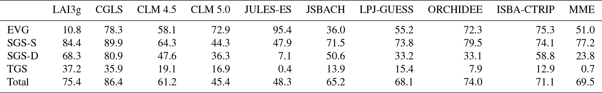
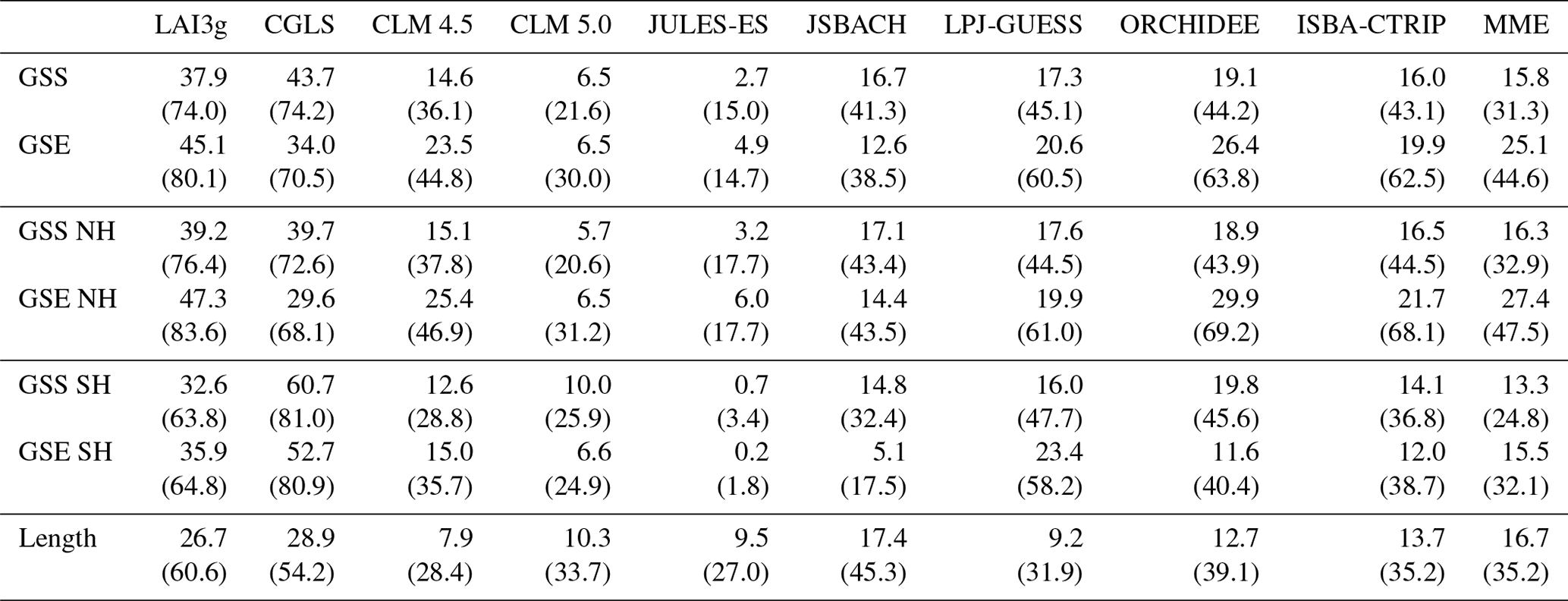
Table 2 The fraction of land grid cell in agreement with MODIS for each satellite product and each land surface model in the four growing season types. Values are reported in percentages and refer to the coloured regions in Fig. 2d and g and Fig. 3.

Larger differences among satellite products are found in the assessment of GSS and GSE (Fig. 2), especially in the NH, where LAI3g and CGLS clearly anticipate GSS (Fig. 2e, h) with respect to MODIS. The three satellite products present a consistency similar to the one reached by the growing-season-type distribution (about 75 %) when a 1-month tolerance is considered (Table 3), since time resolution of the products has been homogenized to 1 month (see Sect. 2.4).

Table 3 The fraction of land grid cell in agreement with MODIS for LAI3g, CGLS, each land surface model, and multi-model ensemble mean (MME) in the growing season start (GSS) and growing season end (GSE) timings. Values are reported in percentages for global, Northern Hemisphere (NH), and Southern Hemisphere (SH). Green shaded areas in Figs. 4 and 5. The last row reports the fraction of land grid cell in agreement with MODIS for each land surface model in growing season length. The values in brackets give the percentage of global, NH, and SH with a maximum difference of 1 month.

Keeping these differences in mind, the MODIS data are used as a graphical reference in Figs. 3, 4, and 5. These figures keep track of the agreement among satellite data despite the choice of MODIS as reference. Figures using CGLS and LAI3g as a graphical reference are presented in the Supplement.

3.2 Growing-season-type distribution

The 4GST allows estimating the ability of each LSM in capturing the observed spatial distribution of the four growing season types (Fig. 3). In general, all the LSMs capture the single growing season that peaks in summer (SGS-S type) reasonably well, especially in the NH mid- and high-latitude regions. The majority of LSMs are also able to correctly represent the two growing seasons (TGS) in the Horn of Africa region (Fig. 3). Most LSMs are unable to reproduce the observed growing-season-type distribution in the SH, except for the evergreen (EVG) tropical areas. A partial exception is LPJ-GUESS, which shows large SGS-S-type areas in South America, Southern Africa, and northern Australia, in agreement with the satellite products (Fig. 3f). The high number of PFTs used by LPJ-GUESS can be the source of this skill (Table 1).

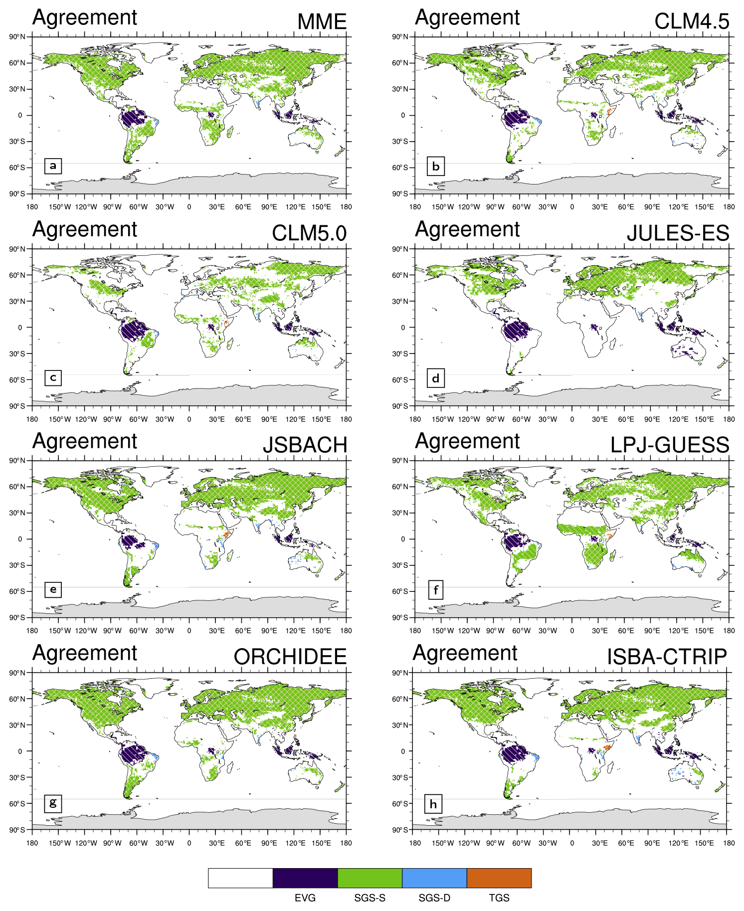
Figure 3 Global climatological (averaged over 2000–2011) distribution of the four main growing season modes for (a) MME, (b) CLM 4.5, (c) CLM 5.0, (d) JULES-ES, (e) JSBACH, (f) LPJ-GUESS, (g) ORCHIDEE, and (h) ISBA-CTRIP. The areas characterized by the same type of LSMs and MODIS (Fig. 2a) are coloured. These common areas are called agreement regions. Index values: (purple) evergreen, (green) single season with summer LAI peak, (cyan) single growing season with summer dormancy, and (orange) two growing seasons type. White regions are for disagreement areas. Above this selection, areas of agreement between satellite products are shaded with a different hatching pattern: MODIS and LAI3g (Fig. 2d) slash hatching ($/$); MODIS and CGLS (Fig. 2g) backslash hatching (\); MODIS, CGLS, and LAI3g crossed hatching (×).

LSMs used in this study are primarily able to capture the observed EVG and SGS-S regions with agreement between 36.0 % and 95.4 % and between 44.3 % and 79.5 %, respectively (Table 2). In contrast, the TGS regions are seldom reproduced by LSMs, and the agreement rate with MODIS ranges between 0.4 % and 19.1 %, (Table 2). Overall, the CRESCENDO multi-model ensemble mean (MME) reproduces the same MODIS growing-season-type distribution over about 69.5 % of global land surface area, with a 45.4 % to 74.0 % range among models (Fig. 3 and Table 2). It is noteworthy that the evergreen type is correctly detected in the broadleaf evergreen tropical areas in both satellite observations and LSMs (Fig. 3). On the contrary, the high-latitude needle-leaf evergreen regions are partially represented in LSMs, while satellite data do not catch these areas due to satellite limitations resulting from the impact of cloud and snow cover on light availability during the winter season (see Sect. 4.2). Besides, the variability of understorey and secondary PFTs may influence LAI seasonality representation.

This initial evaluation highlights that LSMs have difficulties in accurately representing SH phenology. The correct location of the less common types, i.e. single growing season with summer dormancy (SGS-D) and TGS, is as well hardly captured by the LSMs. Similar results are obtained when CGLS and LAI3g satellite observations are used as references (Figs. S2 and S3 and Tables S1 and S2 in the Supplement).

3.3 Variability of growing season start and end

4GST is then applied to evaluate the ability of LSMs to represent the GSS and GSE timing in vegetated areas not classified as EVG type (white regions in Figs. 4 and 5 correspond to not-vegetated and EVG-type domains).

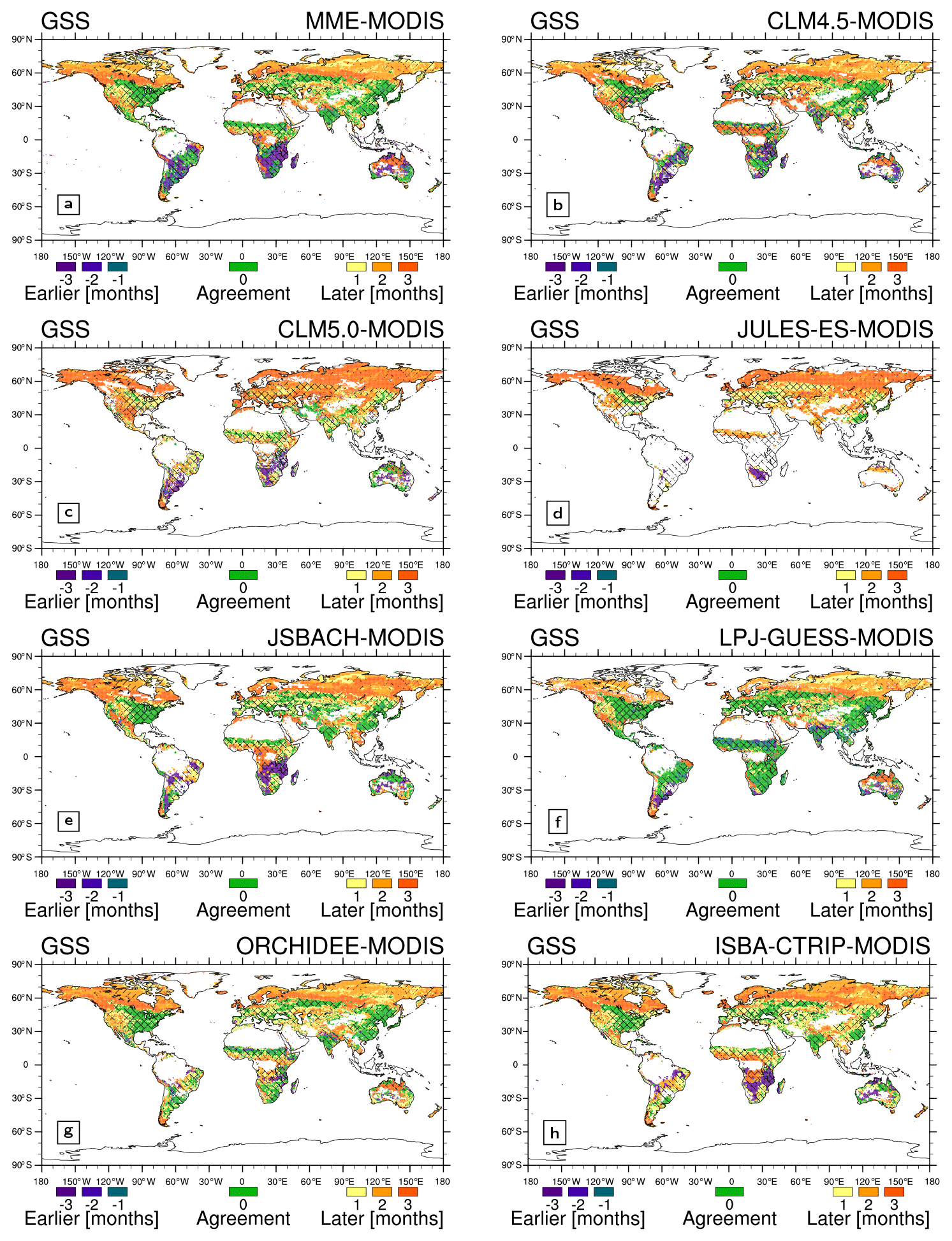
Figure 4 Global climatological (averaged over 2000–2011) differences in the growing season start timings (GSS) between (a) multi-model ensemble mean (MME), (b) CLM 4.5, (c) CLM 5.0, (d) JULES-ES, (e) JSBACH, (f) LPJ-GUESS, (g) ORCHIDEE, and (h) ISBA-CTRIP and MODIS (Fig. 2b). The green regions represent areas of agreement between MODIS and LSMs. Yellow-red colours correspond to areas where models timings are later compared to MODIS, while blue-violet colours correspond to areas where models timings are previously compared to MODIS. Regions where GSS timings are not computed, such as non-vegetated and evergreen areas, are in white. Above this selection, areas of agreement between satellite products are shaded with a different hatching pattern: MODIS and LAI3g (Fig. 2d) slash hatching (/); MODIS and CGLS (Fig. 2g) backslash hatching (\); MODIS, CGLS, and LAI3g crossed hatching (×). Note that the GSS in the TGS regions corresponds to the GSS of the first growing season cycle.

Figure 5 As Fig. 4 but for growing season end (GSE) timings. Note that the GSE in the TGS regions corresponds to the GSE of the second growing season cycle.

On average at the global scale, LSMs approximately exhibit a disagreement of 0.6 months and 0.5 months in GSS and GSE, respectively, with LSMs simulating a later GSS and an earlier GSE, practically shortening the growing season by 1 month (Table 4). This bias is not evenly distributed around the globe. LSMs reproduce the correct growing season length in about 17 % of the global land grid cell, but sometimes the growing season is affected by a shift in seasonality, as in the case of JULES-ES (Table 3). Differently from the other LSMs, the LAI cycle in JULES-ES starts from a climatological condition (Wiltshire et al., 2020a), which can lead to the detected shift.

Table 4 Average difference between MODIS and LAI3g, CGLS, each land surface model, and multi-model ensemble mean (MME) in the growing season start (GSS) and growing season end (GSE) timings. Values are reported in months for global, Northern Hemisphere (NH), and Southern Hemisphere (SH). Positive values stand for later timings, and negative values correspond to earlier timings.

Generally, the GSE timings simulated by the LSMs show a better agreement with MODIS (about 25 % agreement in vegetated grid cell, ranging from 4.9 % to 26.4 %, Table 3) compared to GSS timings (15.8 % agreement in vegetated land grid cell, ranging from 2.7 % to 19.1 %, Table 3). Considering a 1-month tolerance to account for the downgraded time resolution, the agreement between LSMs and MODIS increases to ∼ 45 % and ∼ 31 %, respectively (Table 3).

LSMs exhibit better agreement with MODIS GSS and GSE timings in the NH compared to the SH (Figs. 4 and 5 and Tables 3 and 4). Only CLM 5.0 and LPJ-GUESS show similar results in both hemispheres (Table 3). In particular, LPJ-GUESS shows good skill (agreement with observation larger than 15 %) in capturing both GSS and GSE timings in both hemispheres (Figs. 3f, 4f, and 5f).

LPJ-GUESS is the model that shows the highest agreement with MODIS (Table 3) and the lowest bias in average GSS and GSE timings (0.4 and 0.1 months, respectively, Table 4). JULES-ES shows the lowest agreement with MODIS (Table 3) and the highest bias in the average GSS and GSE timings (1.2 and −2.3, respectively, Table 4). This result may be associated with the representation of PFTs in the two models used to describe global vegetation. LPJ-GUESS, indeed, is the model featuring the largest number of PFTs, while JULES-ES uses the least (Table 1). Moreover, JULES-ES and LPJ-GUESS differ also on the details of the phenology parameterization. LPJ-GUESS features three phenology schemes driven by temperature and soil moisture versus one parameterization only based on the temperature in JULES-ES (Sect. 2.2.3, 2.2.5 and Table 1). Similar to JULES-ES, JSBACH presents a small number of PFTs, but it reaches better results thanks to the five implemented phenology schemes (Sect. 2.2.4 and Table 1).

The two Community Land Model versions (i.e. CLM4.5 and CLM 5.0, Table 3) show very different outcomes, with CLM5.0 exhibiting larger biases in GSS and GSE timings compared to CLM4.5 (Fig. 4b and c, Fig. 5b and c, and Table 4). The two model versions differ in the crop representation, plant physiology, and phenology parameterization (Sect. 2.2 and Table 1). The implementation of an antecedent rain requirement trigger for stress-deciduous PFTs (Dahlin et al., 2015) helps improved phenology in semi-arid regions (e.g. the sub-Sahara, Fig. 4b and c, and Fig. 5b and c). Nonetheless, Zhang et al. (2019) show that the same upgrade influences the leaf senescence in temperate grasslands. On the other hand, the irrigation scheme in the CLM5.0 crop model allows for the improvement in crop-dominated regions, such as the Indian subcontinent (Fig. 4b and c and Fig. 5b and c). Further differences occur between CLM 4.5 and CLM 5.0 (Fig. 4b and c and Fig. 5b and c), which could be ascribed to the changes in plant physiology, soil hydrology, and rooting profile. For example, CLM5.0 applies a different rooting profile scheme and soil moisture threshold (Table 1) affecting the representation of the soil moisture impact on phenology.

CGLS and LAI3g support the results obtained with MODIS in the NH mid-latitude regions, Africa, and Brazil (shaded cross pattern in Figs. 4 and 5). Only LAI3g supports MODIS outcomes in the NH high-latitude regions (shaded slash pattern in Figs. 4 and 5). In general, the direct comparison of LSMs with LAI3g and CGLS satellite observations exhibits results following MODIS ones (Figs. S5–S8 and Tables S3–S6).

3.4 Latitudinal variability

The MME zonal average shown in Fig. 6 highlights the LSMs' abilities and limitations in simulating the observed GSS and GSE timings at different latitudes. The GSS bias ranges between −1.8 months (earlier GSS) just south of the Equator and +2.0 months (delayed GSS) south of 50^∘ S (Fig. 6a). The GSE bias ranges between −3.0 months in the 0–10^∘ N latitudinal band and +1.3 months in the southern sub-tropics. The CRESCENDO LSMs correctly simulate the GSE timings north of 60^∘ N. The Spearman correlation of the GSS and GSE latitudinal distributions is 0.67 ± 0.07 and 0.51 ± 0.11, respectively. These values are significant at the 95 % level based on a Monte Carlo approach.

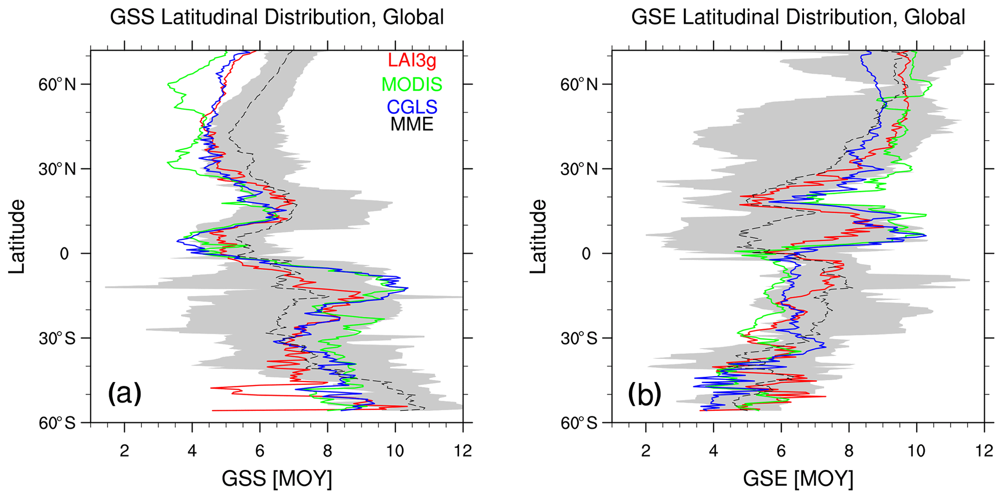
Figure 6 Zonal mean (a) growing season start (GSS) and (b) growing season end (GSE) timings for LAI3g (red lines), MODIS (green lines), CGLS (blue lines), and multi-model ensemble mean (black dashed line). The grey regions show the multi-model ensemble spread. Values are reported as month of the year (MOY), and the latitudinal coverage goes from 56^∘ S to 75^∘ N, which is the range covered by CGLS.

In the NH mid- and high-latitude regions, the LSMs' GSS timings exhibit an average delay of up to 1.6 months, especially in North America (Fig. S9a). This bias and the spread among LSMs might be driven by differences in temperature schemes and thresholds used by LSMs (Table 1). Note that differences among satellite data also occur in the NH mid- and high-latitude regions, highlighting potential differences among these three products (see Sect. 4.2). Large LSM biases in NH tropical region GSE timings and southern sub-tropical GSS timings are driven by premature values in Africa (Fig. S9c, d). These discrepancies may derive from difficulties in the LSM's ability to simulate the observed phenology type and the response to soil moisture in Africa (Figs. 3 and S10). Large variability is spotted in the region below 40^∘ S. The reduced amount of vegetated land area may cause this behaviour. A different growing season type detection in this area, such as a different size of the evergreen region (Fig. 2), may, indeed, extensively influence the GSS and GSE detection, which is the case for the satellite products (Fig. 6), especially LAI3g.

Observed latitudinal distributions highlight an increasing northward trend in the NH mid-latitude GSE timings (GSE around May–June at ∼ 20^∘ N and around September–October at ∼ 40^∘ N, Fig. 6b) and an increasing southward trend in the 30–55^∘ S latitudinal band (GSS around July at ∼ 30^∘ S and around September at ∼ 55^∘ S, Fig. 6a). Similar trends are reproduced by the LSMs, but with a higher magnitude (Fig. 6). In the NH, the difference between simulated and observed trends may be driven by an overestimated influence of radiation and temperature on leaf senescence in LSMs. In the SH, the discrepancies between observed and modelled trends may be related to relatively large phenology variability in the SH associated with the small vegetated land area in this hemisphere.

3.5 Regional variability

To assess sources of biases in the LSMs, different biomes derived from the ESA CCI land cover map (Li et al., 2018, Fig. 7a) are investigated. The GSS timings are generally delayed compared to observations, except for the broadleaf evergreen tree (BET) and broadleaf deciduous shrub (BDS) biomes (Fig. 7f, k). In BDS-dominated regions, the multi-model ensemble mean (MME) falls within the observational range (Fig. 7f, k), but a large spread among LSMs exists. The BDS-dominated regions are semi-arid and transition areas, where LSMs’ parameterization could be more sensitive to climate conditions and parameter selection, especially soil moisture. The large spread among LSMs, then, might be mostly linked to the differences in the implementation of soil moisture in the phenology schemes (Table 1). It is noteworthy that this biome covers a small fraction of the global vegetated regions. The largest biome (i.e. Grass in the Northern Hemisphere, Fig. 7g) instead exhibits a mean delay of 1 month, which is common among the LSMs except for LPJ-GUESS, which falls within observed range. Besides, large biome variability is visible in the SH Crop biome (Fig. 7m). In general, LSMs show a larger variability in the Southern Hemisphere (SH) compared to the Northern Hemisphere (NH).

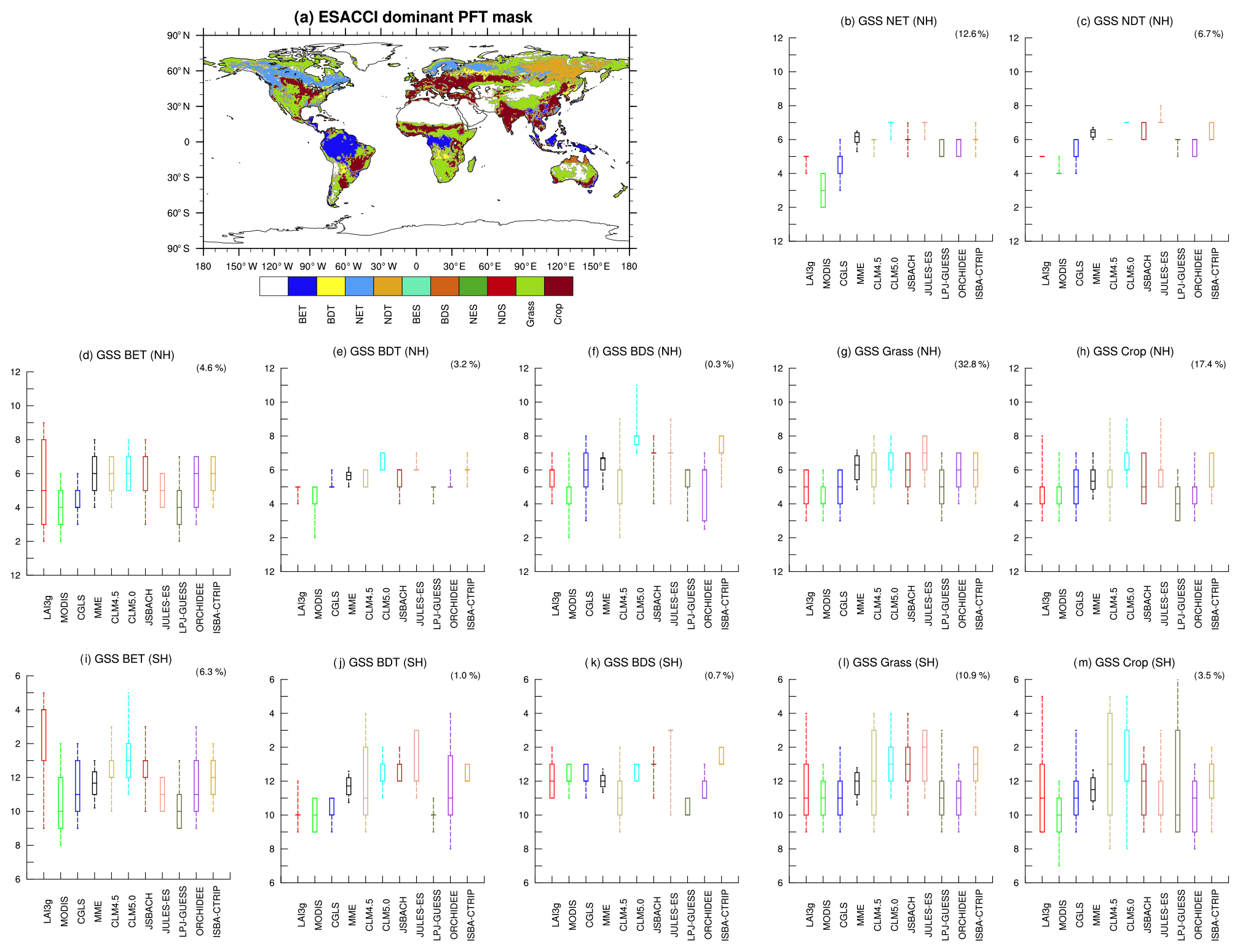
Figure 7 (a) Global distribution of the main land cover types for the 2000–2011 period based on ESA CCI data (Li et al., 2018). Comparison in the growing season start (GSS) timings between satellite products (LAI3g, red; MODIS, green; CGLS, blue) and land surface models (LSMs: MME, black; CLM4.5, dust; CLM5.0, cyan; JSBACH, dark red; JULES, pink; LPJ-GUESS, dark green; ORCHIDEE, purple; ISBA-CTRIP, dark yellow) in (b) needle-leaf evergreen tree (NET) in the Northern Hemisphere (NH); (c) needle-leaf deciduous tree (NDT) in the NH; broadleaf evergreen tree (BET) in the (d) NH and (i) SH; broadleaf deciduous tree (BDT) in the (e) NH and (j) SH; broadleaf deciduous shrub (BDS) in the (f) NH and (k) SH; grass-covered areas (Grass) in the (g) NH and (l) SH; and crop-covered areas (Crop) in the (h) NH and SH (m). Note that no area is dominated by broadleaf evergreen shrub (BES), needle-leaf evergreen shrub (NES), or needle-leaf deciduous shrub (NDS) biome. The boxplots represent the median, 25/75th percentile, and 10/90th percentile of the distribution of grid points belonging to each biome illustrated in panel (a). Each panel shows in parentheses the percentage of global vegetated area covered by each biome. Note that the y axis is different in the NH and SH panels, but in both cases the summer season is central along the axis.

GSE timings display heterogeneous outcomes (Fig. 8). In general, a larger variability is observed compared to GSS timings. The NH Grass biome, which covers about 33 % of the global vegetated area, exhibits a mean delay of 1 month which is mainly driven by JULES-ES (Fig. 8g). The SH BDS area displays a large variability among models (Fig. 8k) ranging from May (LPJ-GUESS) to November (JULES-ES). Large biome variability appears in broadleaf evergreen tree (BET), Grass and Crop SH biomes (Fig. 8i, l, m), and NH Crop (Fig. 8h). This result highlights the need for further investigation on the representation of crop phenology in the LSMs since only a few LSMs (i.e. JSBACH and ORCHIDEE) treat crops with a specific parameterization (Sect. 2).

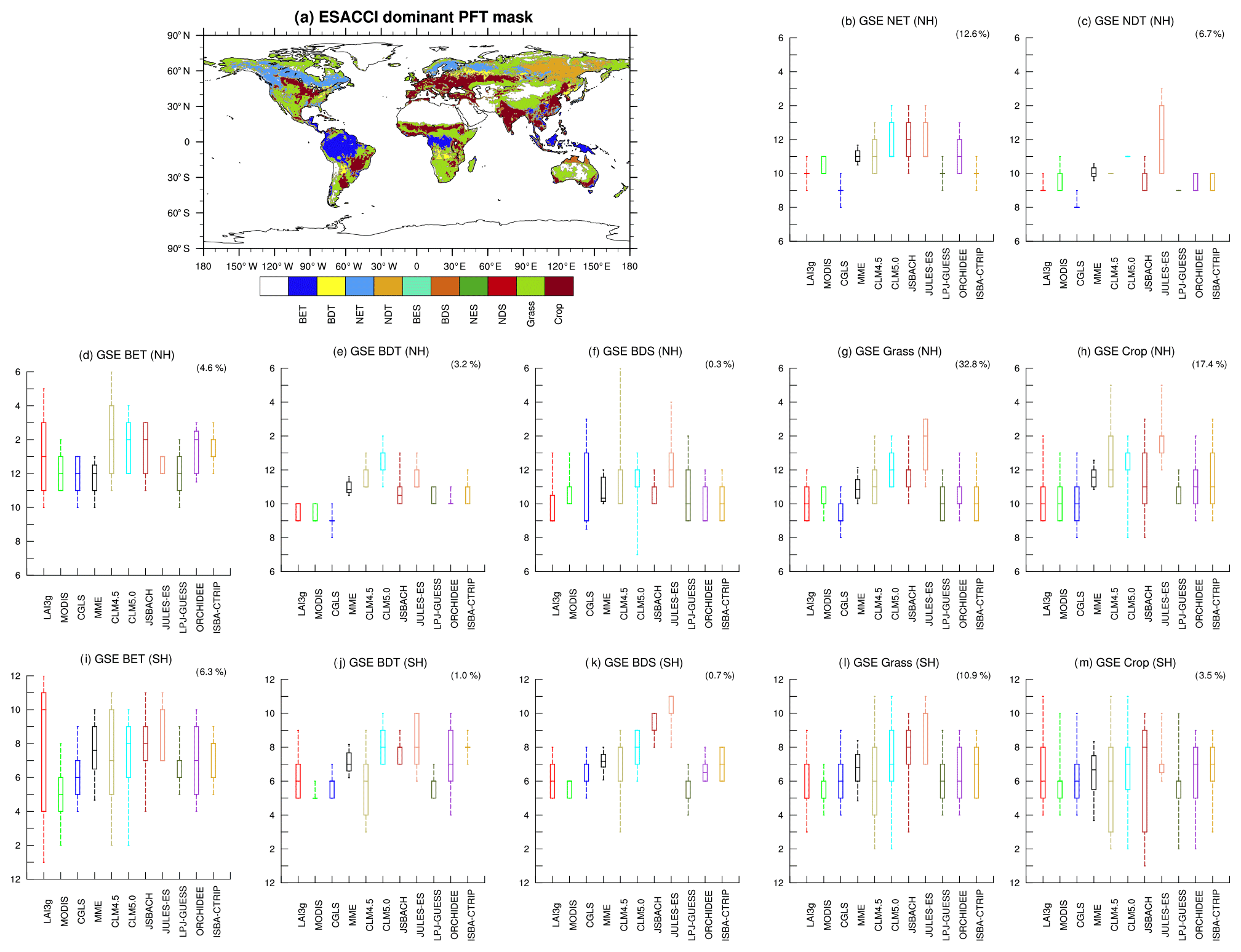
Figure 8 As Fig. 7 but for growing season end (GSE) timings. In this case, the winter season is central along the y axis.

In general, LSMs show a higher agreement in representing GSS timings compared to GSE timings. Consequently, the different approaches used to describe the start of the growing season are relatively consistent among LSMs. In comparison, the representation of the end of the vegetative season requires further investigation and development. Note that this regional evaluation is performed based on the observed biome distribution (i.e. ESA CCI map). However, each LSM treats differently the land cover and biome distribution (Sect. 2). For this reason, part of the obtained spread among LSMs derives from differences in PFT representation and distribution (Sect. 2.2, and Table 1), which affect phenology representation in LSMs.

4 Discussion

4.1 Land surface models

The plant phenology growing season start and end are mainly triggered by changes in solar radiation, temperature, and soil moisture conditions (e.g. Caldararu et al., 2012; Zeng et al., 2013; Tang and Dubayah, 2017). State-of-the-art LSMs represent the phenological transitions using different parameterizations based on the climate conditions (Sect. 2.2). Many of these parameterizations (see Sect. 2.2) are based on values derived from localized observations (e.g. White et al., 1997; Thornton et al., 2002; Jolly et al., 2005; Savoy and Mackay, 2015). Consequently, the phenology parameters are calibrated on specific regions of the globe, which may be one reason for the large spread of values seen in the present analysis.

Generally, phenology calibration areas are located in the NH, where LSMs exhibit better results and larger coherence compared to the SH. Among the LSMs evaluated here, LPJ-GUESS, CLM4.5, and ORCHIDEE show good skill (agreement with observation larger than 15 %) in the SH (Table 3). On the other hand, CLM5.0 and JULES-ES do not reach such agreement in the NH (Table 3). High skill (agreement with observation larger than 20 % for at least one timing) in the NH is obtained by CLM4.5, ORCHIDEE, and ISBA-CTRIP (Table 3). The different performance between models can occur from differences in phenology parameterization as well as different vegetation cover types (plant and crop functional types), soil characterization, and initial spatial resolution (Table 1).

Among the LSMs evaluated here, JULES-ES shows relatively lower skill in simulating GSS and GSE timings compared to the other LSMs (Table 3). This result may be ascribed to the smaller number of PFTs (see Table 1) and details of the phenology parameterization that characterize this LSM (Sect. 2.2.3 and Table 1). JSBACH accounts for a similar number of PFTs (Table 1) but features a more complex phenology scheme (Sect. 2.2.4 and Table 1). For this reason, JSBACH exhibits a higher skill than JULES-ES in reproducing GSS and GSE timings (Table 3).

Similar to JSBACH, ORCHIDEE features a PFT-oriented phenology scheme (Sect. 2.2.6 and Table 1), which contributes to the high skill noted for ORCHIDEE.

CLM 4.5, CLM 5.0, and LPJ-GUESS use three phenology schemes: (1) evergreen, (2) seasonal deciduous, and (3) stress deciduous (Sect. 2.2.1, 2.2.2, 2.2.5). Among these schemes, the seasonal deciduous one employs calendar thresholds (summer and winter solstices and day length threshold in CLM, and fixed 210 d phenology in LPJ-GUESS) that may improve the results of LPJ-GUESS and CLM 4.5. On the other hand, this may mean that the seasonal-deciduous type may be less responsive to future climate change.

Contrary to the other LSMs, ISBA-CTRIP uses the daily leaf carbon balance to simulate plant phenology, and it reaches good skill (Tables 3, 4). Consequently, ISBA-CTRIP highlights the opportunity to attain results aligned with the other LSMs using leaf carbon availability instead of climatic conditions.

The improvement of the phenology parameterization can lead to better representation of vegetation in the LSMs. However, other vegetation features affect the plant phenology representation, as in the case of the two CLM versions. CLM4.5 and CLM5.0 share similar phenology parameterization (Sect. 2.2.1 and 2.2.2) but differ in the crop irrigation scheme, soil and plant hydrology, and carbon and nitrogen cycling (Lawrence et al., 2018). Since soil moisture has a significant control on plant phenology (e.g. Caldararu et al., 2012), the CLM5.0 revision of stomatal response to rising CO₂ concentrations through a new Medlyn stomatal conductance scheme (Fisher et al., 2019; Medlyn et al., 2011) and the use of a revised mechanistically based soil evaporation parameterization that accounts for the rate of diffusion of water vapour through a dry surface layer (Swenson and Lawrence, 2014) are likely to be principal sources of differences between CLM5.0 and CLM4.5.

In general, this comparison highlights the complexity of vegetation phenology modelling and the strong interlinkage between climate, hydrology, soil, and plants.

4.2 Satellite data

Satellite-based LAI datasets have been used in this work as a benchmark for the evaluation of the LSMs' phenology performance globally. However, satellite observations present some caveats and uncertainties (e.g. Myneni et al., 2002; Fang et al., 2013; Jiang et al., 2017). For this reason, three separate satellite LAI products obtained from different acquisition sensors (namely AVHRR for LAI3g, MODIS for MODIS LAI, and SPOT/PROBA VEGETATION for CGLS) have been used in this study. The comparison between these datasets shows major issues associated with LAI products derived from satellite reflectance observations. For example, large differences between LAI3g, MODIS, and CGLS occur at high latitudes and in tropical regions (Fig. 6), where thick clouds and snow cover can affect the data reconstruction (e.g. Delbart et al., 2006; Kandasamy et al., 2013; Yan et al., 2016b). LAI satellite data are also affected by the applied regridding and gap-filling algorithms, which could create spurious seasonal cycles as well as smooth the observed phenology season (e.g. Kandasamy et al., 2013; Chen et al., 2017). In addition, the observed reflectance saturates in regions characterized by dense canopies reaching prescribed LAI upper limits (e.g. 7.0 m² m⁻² in MODIS and LAI3g  Myneni et al., 2002; Maignan et al., 2011). This issue can affect the identification of growing season cycles in thickly forested areas, leading to possible overestimation of evergreen type detection.

4.3 4GST limitations

Contrary to previous phenology analysis that focused on specific biomes (e.g. Dahlin et al., 2015; Zhang et al., 2019) or NH mid- and high-latitude regions (above 30^∘ N Anav et al., 2013; Murray-Tortarolo et al., 2013), 4GST accounts explicitly for different phenology types on the global scale. In particular, it takes into account SGS-D and TGS types that were neglected in previous analyses (Murray-Tortarolo et al., 2013) due to their reduced coverage (Table 2).

Regions with multiple growing seasons per year (TGS) are difficult to capture on a global scale, despite their important influence on climate (e.g. Zhang et al., 2003; Dalmonech and Zaehle, 2013; Peano et al., 2019). The state-of-the-art LSMs, indeed, exhibit a low skill in reproducing this specific growing season type (Fig. 3 and Table 2). Two growing seasons usually occur in regions characterized by two separate rain seasons, in semi-arid areas, or in cropland regions (e.g. Zhang et al., 2003, 2005; Martiny et al., 2006). In this analysis, observations and LSMs, except for JULES-ES and ORCHIDEE, agree on a TGS type only in the Horn of Africa. This region features two distinct precipitation seasons (e.g. Liebmann et al., 2012; Peano et al., 2019), which trigger the TGS phenology type.

Cropland areas can present multi-growing-season behaviour because of irrigation and crop rotation, such as in South Asia and China (e.g. Wu et al., 2010; Gumma et al., 2016). Unlike the Horn of Africa, these regions are not captured as TGS in the present analysis due to assumptions and limitations within LSMs – for example CLM4.5 represents all annual crops by a generic C₃ PFT (Sect. 2.2.1 and Table 1) – and 4GST assumptions. 4GST TGS type detection adopts a minimum length of 3 months to detect a growing season. This assumption derives from the need to avoid the detection of small oscillations within the same growing seasons (Peano et al., 2019). Consequently, this assumption affects the model recognition of multiple growing seasons, especially in cropland areas. South Asia, for instance, is characterized by different timing and phenology intensity for each crop growing season (Gumma et al., 2016). Therefore, only some specific crops can be detected based on the 4GST assumptions and growing season signature (Gumma et al., 2016). Wu et al. (2010) distinguish multiple growing seasons in China using the local maximum and detection threshold. This method improves the multi-growing-season identification, especially for the crops identified by a strong phenology cycle, but may exclude crop characterized by a weak phenological cycle. For these reasons, more specific analyses of semi-arid and crop regions based on higher spatial and temporal data are needed and will be the focus of a future study. Besides, LSMs' crop phenology parameterizations require further development to improve the description of each specific crop.

Another limitation of the present evaluation is the monthly temporal frequency. Data at a higher frequency, indeed, might lead to a more detailed bias assessment. The use of a different temporal frequency may also influence phenology type detection. For example, Peano et al. (2019), who use 15 d LAI data, detect a slightly different distribution of CLM4.5 SGS-D and TGS types in Australia, the Horn of Africa, and Brazil. Similarly, Zhang et al. (2019), who analyse CLM4.5 in northeast China with 8 d LAI data, obtain TGS type in areas recognized as SGS-S in the present analysis.

LSMs evaluate phenology at the PFT level, but the final LAI values are returned at the grid-cell level. For this reason, a more detailed evaluation of the parameterization would require using PFT-level values. However, global coverage of observed PFT-level phenology values is missing, making this analysis limited to specific biomes, such as through PhenoCam data (Richardson et al., 2018). This analysis will be the focus of a future work.

5 Conclusions

This study evaluates the ability of the land component (LSMs) of seven state-of-the-art European Earth system models participating in the CMPI6 to reproduce the timings of the start and end of the plant growing season at the global level. The assessment is performed based on the novel four growing season types methodology and uses a set of three satellite observation products as a benchmark to account for some of the uncertainty in observations.

In general, LSMs exhibit better agreement with observations in the NH compared to the SH, where large variability associated with the small vegetated land area is present. LSMs also show higher ability to simulate the timing of the growing season end compared to the timing of the growing season start. On average, LSMs show a 0.6-month delay in estimating the start of the growing season and about a 0.5-month premature in estimating the end of the growing season, leading to about a 1-month-shorter phenology active season. High discrepancies between LSMs and satellite products are noted for growing season start (GSS) timings in the region poleward of 50^∘ S, where simulated GSS is delayed by about 2 months. The growing season end (GSE) shows high differences between LSMs and observations in the 0–10^∘ N latitudinal band, where LSMs simulate a 3-months-earlier GSE. On the contrary, the LSMs accurately simulate the GSE timings poleward of 60^∘ N and the GSS in the 30–40^∘ S and 10–30^∘ N latitudinal bands. At the biome scale, LSMs correctly simulate the GSS and GSE timings in broadleaf-evergreen-tree-dominated areas. High intra-model variability remains in the broadleaf-deciduous-shrub- and Crop-dominated areas.

Despite a lower ability of LSMs to represent SH phenology, LPJ-GUESS, CLM4.5, and ORCHIDEE show reasonably good outcomes in these regions. In the NH, high skill is achieved by CLM4.5, ORCHIDEE, and ISBA-CTRIP. Uncertainties and spread among LSMs remain, which might affect our understanding of present-day and future impact of land and vegetation interactions with the climate and carbon cycle. Therefore, further improvements in LSMs will be necessary.

Improvements in the phenology parameterization can lead to better representation of vegetation in the LSMs. However, phenology in LSMs is influenced by vegetation and hydrological parameterizations and land surface boundary conditions (e.g. PFT distribution), as shown by the CLM4.5 and CLM5.0 phenology differences.

This study highlights the complexity of vegetation phenology modelling and the strong interlinkage between climate, hydrology, soil, and plants, which need further details and generalization inside the LSM code.