Upwelling-induced trace gas dynamics in the Baltic Sea inferred from 8 years of autonomous measurements on a ship of opportunity

Autonomous measurements aboard ships of opportunity (SOOP) provide in situ data sets with high spatial and temporal coverage. In this study, we use 8 years of carbon dioxide (CO₂) and methane (CH₄) observations from SOOP Finnmaid to study the influence of upwelling on trace gas dynamics in the Baltic Sea. Between spring and autumn, coastal upwelling transports water masses enriched with CO₂ and CH₄ to the surface of the Baltic Sea. We study the seasonality, regional distribution, relaxation, and interannual variability in this process. We use reanalysed wind and modelled sea surface temperature (SST) data in a newly established statistical upwelling detection method to identify major upwelling areas and time periods. Large upwelling-induced SST decrease and trace gas concentration increase are most frequently detected around August after a long period of thermal stratification, i.e. limited exchange between surface and underlying waters. We found that these upwelling events with large SST excursions shape local trace gas dynamics and often lead to near-linear relationships between increasing trace gas levels and decreasing temperature. Upwelling relaxation is mainly driven by mixing, modulated by air–sea gas exchange, and possibly primary production. Subsequent warming through air–sea heat exchange has the potential to enhance trace gas saturation. In 2015, quasi-continuous upwelling over several months led to weak summer stratification, which directly impacted the observed trace gas and SST dynamics in several upwelling-prone areas. Trend analysis is still prevented by the observed high variability, uncertainties from data coverage, and long water residence times of 10–30 years. We introduce an extrapolation method based on trace gas–SST relationships that allows us to estimate upwelling-induced trace gas fluxes in upwelling-affected regions. In general, the surface water reverses from CO₂ sink to source, and CH₄ outgassing is intensified as a consequence of upwelling. We conclude that SOOP data, especially when combined with other data sets, enable flux quantification and process studies addressing the process of upwelling on large spatial and temporal scales.

1 Introduction

Coastal upwelling areas are known to be hotspots of greenhouse gas emissions from marine systems to the atmosphere (Capelle and Tortell, 2016; Morgan et al., 2019). This is a result of (1) enhanced productivity and mineralisation; (2) often hypoxic conditions in the subsurface waters leading to increased concentrations of reduced compounds such as CH₄, N₂O, ${\mathrm{NH}}_{\mathrm{4}}^{+}$, or H₂S; and (3) an effective transport mechanism of these subsurface waters to the air–sea interface. Climate change is expected to have an amplifying effect on the intensity of coastal upwelling in the global ocean (Bakun et al., 2015; Xiu et al., 2018). Eutrophication and reduced ventilation lead to the spreading and intensification of hypoxia in coastal systems (Diaz and Rosenberg, 2008). The combination of these effects will undoubtedly affect the trace gas dynamics in upwelling regions.

The Baltic Sea – a brackish, semi-enclosed sea in northern Europe (Fig. 1) – is among the fastest-warming marginal seas worldwide (Kniebusch et al., 2019). It is further known to be strongly affected by environmental changes such as eutrophication (HELCOM, 2018), changing wind patterns, and thus upwelling intensity (BACC II Author Team, 2015) and has also been shown to encounter a decrease in oxygen at a large number of coastal sites over the last decades (Caballero-Alfonso et al., 2015). As a result of these ongoing, strong changes, the Baltic Sea offers the potential to study feedbacks between anthropogenic and climatic drivers and upwelling-induced greenhouse gas fluxes earlier and with a higher signal intensity compared to regions that just start transforming due to climate change. For instance, “time of emergence” studies suggest that the influence of anthropogenic carbon uptake will not be observable until between 2020 and 2050 in most parts of the global ocean (McKinley et al., 2016).

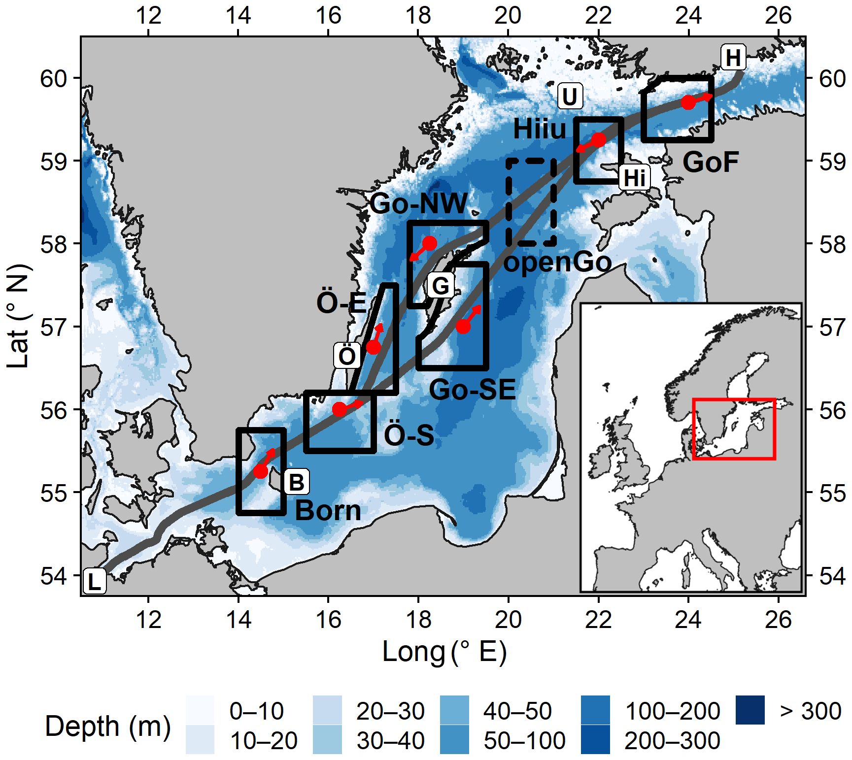
Figure 1 Map and bathymetry of the study area with typical routes of SOOP Finnmaid (grey) between Lübeck–Travemünde (L) and Helsinki (H). Boxes highlight seven regions (solid lines) in which we expect upwelling to occur and one in the open Gotland Sea (dashed lines) as a reference (Table 1). Red dots mark the locations of wind data used for this study, with red arrows indicating upwelling-favourable wind directions. We further marked the islands of Bornholm (B), Öland (Ö), Gotland (G), Hiiumaa (Hi), and Utö (U).

The Baltic Sea is characterised by riverine inflow of fresh water from a large drainage basin and inflows of seawater from the North Sea, which, together with its basin structure, results in a permanent vertical salinity and density stratification (Feistel et al., 2010). A shallow surface thermocline is present during summer, and large parts of the Baltic Sea are additionally characterised by a permanent halocline, with hypoxic or even anoxic water underneath (Fig. 2). The typical seasonality of surface carbon dioxide (CO₂) partial pressure (pCO₂) in the Baltic Sea features a minimum during spring and one or more subsequent minima throughout summer: the spring bloom starts in March/April with the formation of the surface thermocline and peaks in mid-May (Schneider and Müller, 2018). Pulses of mid-summer bloom events are driven by nitrogen fixation (Schneider et al., 2014a); pCO₂ slightly increases in between due to warming, air–sea exchange, and remineralisation of organic matter (Schneider et al., 2014b). Beginning in September/October, deepening of the mixed layer leads to increasing pCO₂ in the surface water as a consequence of entrainment of deeper waters that have been subject to organic matter remineralisation (Schneider et al., 2014a). Typical pCO₂ values in the central Baltic Sea range from about 100 to 500 µatm (Schneider et al., 2014a), and undersaturation is usually observed from March/April to September/October, depending on region (Schneider and Müller, 2018).

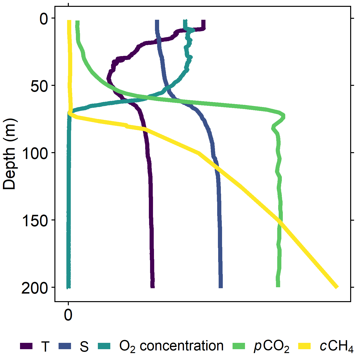
Figure 2 Vertical profiles of parameters relevant for this study from 58.58^∘ N, 18.23^∘ E, on 23 May 2019, which show shapes typical for the summer situation in the central Baltic Sea. The profiles display temperature, salinity, oxygen concentration, CO₂ partial pressure, and CH₄ concentration on an arbitrary scale, truncated at a depth of 200 m.

The methane (CH₄) distribution in the Baltic Sea is mainly governed by the vertical redox and density stratification (Fig. 2): anoxic, CH₄-enriched bottom water in the deep basins and CH₄ oxidation in the water column, especially in the redox zone located slightly below the permanent halocline (Jakobs et al., 2013), lead to strong vertical gradients and concentrations near atmospheric equilibrium in the surface water (Schmale et al., 2010; Jakobs et al., 2013). CH₄ is also produced in the upper, oxic water column (Jakobs et al., 2014; Schmale et al., 2018), partially by zooplankton (Schmale et al., 2018; Stawiarski et al., 2019). The Baltic Sea acts as a permanent source of atmospheric CH₄. The highest CH₄ emissions to the atmosphere are observed in the Gulf of Finland in winter (Gülzow et al., 2013) and in the shallow western basins due to CH₄-rich sediments (Schmale et al., 2010).

Local coastal upwelling increases both pCO₂ and CH₄ concentration (cCH₄) in the surface water of the Baltic Sea by introducing enriched water from below the summer thermocline (Fig. 2) to the surface (Gülzow et al., 2013; Norman et al., 2013; Schneider et al., 2014b; Humborg et al., 2019; Stawiarski et al., 2019). However, since previous studies were limited to episodic events, only little is known about the seasonality and regional distribution of upwelling-induced trace gas signals in the Baltic Sea and their relaxation. Ferry-based measurements enable studies on upwelling in the Baltic Sea on larger scales, which has already been demonstrated for physical parameters in the Gulf of Finland (Kikas and Lips, 2016).

Upwelling events in the Baltic Sea are common but irregular since they depend on wind conditions (Lehmann and Myrberg, 2008). Westerly to south-westerly winds prevail in the Baltic Sea area, which enhances the possibility of upwelling near southern and south-eastern coasts (see red arrows in Fig. 1). These upwelling events have a typical lifetime of several days up to 1 month with sharper horizontal gradients compared to oceanic upwelling (Lehmann and Myrberg, 2008). In summer, sea surface temperature (SST) may decrease by more than 10 ^∘C during an upwelling event, while salinity changes are usually below 0.5 (Lehmann and Myrberg, 2008). The influence of upwelling decreases in autumn and winter, when no seasonal stratification is present. While for oceanic upwelling regions, it is known that upwelling may trigger extreme primary production through nutrient transport, the influence of upwelling on primary production in the Baltic Sea is still poorly constrained (Lehmann and Myrberg, 2008). However, upwelled waters characterised by low nitrogen$/$phosphorus ratios have been reported to fuel cyanobacteria blooms during nitrogen limitation (Vahtera et al., 2005; Lips et al., 2009; Wasmund et al., 2012). Yet, time lags of about 3 weeks have been reported for this feedback with an initial decline in phytoplankton biomass (Vahtera et al., 2005; Wasmund et al., 2012). As an explanation for this delay, Wasmund et al. (2012) propose that the initialisation of a cyanobacteria bloom requires mixing of biomass-rich surface water with phosphate-rich upwelled water.

The quantification of dissolved greenhouse gases like CO₂ and CH₄ across large spatial and temporal scales is critical to derive accurate climate projections (Friedlingstein et al., 2019) and helps to understand processes involved in the biogeochemical cycling of both gases (Takahashi et al., 2009). The latter also necessitates high spatial and temporal resolution in environments with strong spatial or temporal gradients (Webb et al., 2016). Traditional research cruises usually involve discrete sampling in the water column and often continuous surface water measurements using an air–water equilibrator coupled to nondispersal infrared spectroscopy for CO₂ (e.g. Körtzinger et al., 1996), gas chromatography for CH₄ (e.g. Bange et al., 1994), or cavity-enhanced absorption spectroscopy (CEAS; e.g. Gülzow et al., 2011; Du et al., 2014) – a relatively new technique with high sensitivity for both gases (Gagliardi and Loock, 2014). Whereas research cruises enable vertically resolved measurements in a certain region over several weeks, they do not provide wide temporal and sometimes spatial coverage, which is the main advantage of autonomous measurements aboard ships of opportunity (SOOPs). SOOP data sets enable studies with a broader perspective that – unlike remote sensing and modelling – are still based on in situ measurements. While SOOP-based CO₂ measurements are common owing to the available hardware (Pierrot and Steinhoff, 2019), CH₄ measurements are still scarce due to the comparatively recent development of CEAS and the elaborate set-up aboard a SOOP (Gülzow et al., 2011; Nara et al., 2014). The ferry and SOOP Finnmaid hosts such an autonomous set-up measuring surface concentrations of dissolved CO₂ and CH₄ since late 2009 using a CEAS sensor (Gülzow et al., 2011), resulting in a unique long-term data set. The vessel transects the Baltic Sea between Lübeck–Travemünde (Germany) and Helsinki (Finland) about four times per week (Fig. 1). SOOP Finnmaid is part of the German contribution to the European ICOS (Integrated Carbon Observation System) research infrastructure.

The large extent to which the Baltic Sea is influenced by climatic and anthropogenic forces and the availability of the presented 8-year data set of SOOP Finnmaid and of high-resolution models (Placke et al., 2018; Gräwe et al., 2019) make the Baltic Sea a unique study site to detect feedbacks early and to develop methods and process understanding that can be used to analyse long-term data sets with respect to, for example, upwelling-induced trace gas dynamics. The SOOP strategy allows us to investigate the influence of coastal upwelling on surface pCO₂ and cCH₄ in the Baltic Sea on a large spatial and temporal scale without issues of bad coverage of seasonality due to (biased) individual research-vessel-based studies. Furthermore, methods developed here can possibly be used for the treatise of upwelling in other regions. Depending on their size and on the frequency and magnitude of upwelling, these may be more important for global trace gas fluxes and budgets compared to the Baltic Sea, e.g. in the case of the large eastern-boundary upwelling systems. In this study, we

• present a method to identify upwelling events along the SOOP track based on wind and modelled SST data

• compare upwelling-induced trace gas dynamics within several regions in the Baltic Sea

• examine the relaxation of upwelling events over time

• discuss interannual variability within the data set and highlight the importance of upwelling to understand CO₂ and CH₄ dynamics in the Baltic Sea

• evaluate whether a long-term trend can be inferred from the analysis of this 8-year data set taking into account the interannual variability, and

• demonstrate the potential of extrapolating trace gas observations based on modelled SST data

with the aim of

• assessing the prevalence of upwelling and attributing observed trace gas signals to upwelling

• revealing regional characteristics

• explaining frequently observed features during and after upwelling events with a focus on underlying processes

• identifying controlling mechanisms of seasonality and variability, and

• showing ways to estimate air–sea trace gas fluxes on a broader spatial scale under extremely variable conditions, which may be a useful method for other upwelling areas worldwide.

We present most of the findings by use of illustrating examples but provide more information in the Appendix, Supplement, and data set.

2 Data and methods

2.1 Measurements aboard SOOP Finnmaid

SOOP Finnmaid is equipped with a variety of sensors to survey the surface water of the Baltic Sea between Lübeck–Travemünde in Germany and Helsinki in Finland (Fig. 1). Parameters including SST, salinity, pCO₂, and cCH₄ are logged every minute. The data set used for this study refers to the time period from May to September and the regions defined in Table 1 and consists of 482 transects from 2010 to 2017.

Table 1 Upwelling areas crossed by SOOP Finnmaid (abbreviated and long name); their boundaries (latitude and longitude), including a specification if the respective box is not rectangular (Fig. 1); their upwelling-favourable (upw.-fav.) wind direction; and the distance between the track of SOOP Finnmaid within the box and the coast, given as median (med.) and minimum (min.). This distance is calculated perpendicular to the upwelling-favourable wind direction and based on an average track.

^a Wind directions in brackets have been considered but were found to have only little influence on data from SOOP Finnmaid.
^b Due to large distances to surrounding coasts.
^c Calculated as nearest coast in any direction.

The on-board trace gas measurement system consists of a Los Gatos Research CH₄ and CO₂ analyser coupled with an air–water equilibrator (Körtzinger et al., 1996), which is described in detail in Schneider et al. (2014b) and Gülzow et al. (2011, 2013), including details on the following calculations: the measured variables are the mole fractions xCO₂ and xCH₄ in parts per million, which are corrected to dry-air values using xH₂O data from the same instrument. These mole fractions are converted into partial pressures using atmospheric pressure data and calculating saturation water vapour pressure following Weiss and Price (1980) under the assumption of 100 % humidity in the equilibrator headspace. In literature, CO₂ data are usually reported as partial pressure or fugacity, while CH₄ data are converted into concentrations. Accordingly, we report pCO₂ and cCH₄; the latter was calculated from the partial pressure (pCH₄) using Bunsen solubility coefficients determined by Wiesenburg and Guinasso (1979). Note that we can handle the concentration (of CH₄ in nmol L⁻¹) as a quasi-conservative parameter with respect to temperature changes in the discussion as the influence of temperature on water density is negligible in this case. In contrast, the partial pressure (of CO₂) in equilibrium with the water phase is temperature-dependent (see also Sect. 3.3). To compensate the effect of water warming from inlet to equilibrator, pCO₂ is temperature-corrected following Takahashi et al. (1993). The data set was not corrected for equilibrator response times, which especially affect CH₄ measurements due to its poor solubility (Webb et al., 2016), for reasons detailed in Sect. A2.

We post-calibrated xCO₂ and xCH₄ using a single-point calibration to a standard gas at near-atmospheric mole fractions. These standard gas measurements were performed automatically when leaving the harbour to yield a drift correction between transects. The measurement system aboard SOOP Finnmaid also includes a LI-COR 6262 CO₂ and H₂O analyser with a separate equilibrator. Even though these additional CO₂ data are not presented here, they provided cross-validation and quality control. Presenting both CO₂ and CH₄ measurements from the same instrument ensures the best consistency between the two trace gases. Therefore, minor deviations from the previously published CO₂ data set in SOCAT (Surface Ocean CO₂ Atlas; https://www.socat.info, last access: 31 August 2020, Bakker et al., 2016) exist, which is a combined product of both set-ups. In the study area and period, these differences in pCO₂ have a median of 0.75 µatm and an interquartile range (IQR) of 2.1 µatm.

We further used monthly averaged atmospheric CO₂ and CH₄ data to calculate atmospheric-equilibrium conditions. For the closest distance to observations from SOOP Finnmaid, we utilised atmospheric data from Utö station (Finnish Meteorological Institute, Helsinki) starting in March 2012. Prior to that or to fill gaps in the Utö series, atmospheric data from Mace Head station (National University of Ireland, Galway) via the NOAA Earth System Research Laboratories (ESRL) carbon cycle cooperative global air sampling network (Dlugokencky et al., 2019a, b) were used, and both data sets were matched to those of Utö by linear regression (Fig. A2 for details). The atmospheric data are displayed as atmospheric partial pressure for CO₂ or as equilibrium concentration calculated from SST and salinity for CH₄. We also plotted relative CH₄ saturation, which is the ratio of cCH₄ to equilibrium concentration.

2.2 Wind and modelled SST data

Wind-induced upwelling in summer results in decreasing SST. Thus, to attribute trace gas signals in the data set of SOOP Finnmaid to upwelling and to assess the spatial and temporal dimensions of upwelling events, we combined reanalysed wind and modelled SST data to locate upwelling events in space and time before starting the actual in situ data analysis. Using modelled SST data enabled us to also identify events that SOOP Finnmaid missed. We found that model-derived SST data were more suitable than remote-sensing-derived SST data, which are subject to, for example, cloud coverage.

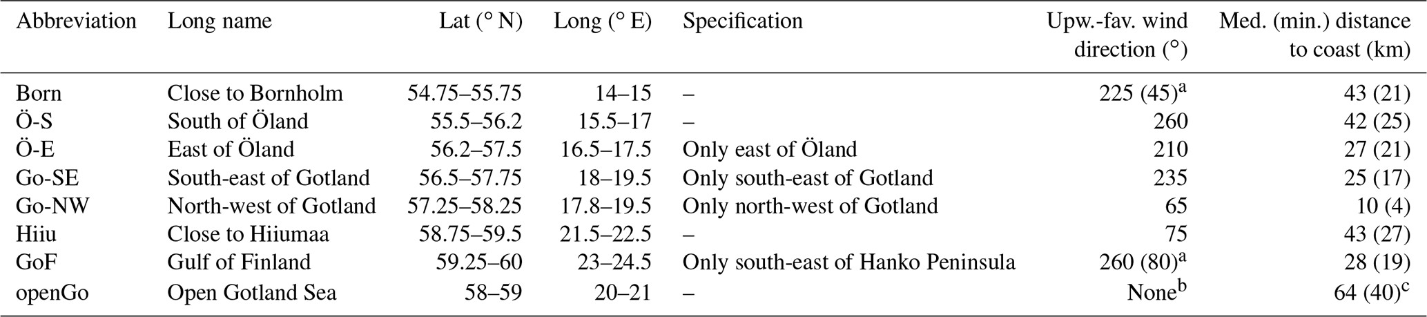
We used the SST output of the numerical ocean model GETM (General Estuarine Transport Model) for the Baltic Sea. The model has a horizontal resolution of 1 nmi and 50 vertical terrain-following levels. The uppermost level has a maximum thickness of 50 cm to properly represent the SST and ocean–atmosphere fluxes. The model run covers the period from 1961 to 2019. For a detailed analysis of the model performance see Placke et al. (2018) and Gräwe et al. (2019). For the present run, we restarted the model in 2003 but changed the atmospheric forcing to the operational reanalysis data set of the German Weather Service (DWD), with a spatial resolution of 7 km and a temporal resolution of 3 h (Zängl et al., 2015). The same wind data – extracted for one location per upwelling region, respectively (Fig. 1) – were used to identify upwelling events (Sect. 2.3). To give an impression of the model performance, Fig. 3 and Animation S1 in the Supplement illustrate SST in the Baltic Sea during a strong upwelling event taken from both the model and a multi-sensor level 3 SST remote sensing product for the European seas (Copernicus, 2020). This comparison demonstrates both good agreement and the advantage of model data due to insensitivity to cloud coverage. Differences between modelled SST data along the track of SOOP Finnmaid and shipboard SST observations in the entire study area and period have a median of 0.04 ^∘C and an IQR of 1.41 ^∘C. Differences between model and observations partly result from different timescales, i.e. daily means (model data) vs. real time (in situ data).

Figure 3 SST in the Baltic Sea on 16 August 2016 (daily mean) as extracted from (a) the model and (b) the remote sensing product (see text). SST measurements aboard SOOP Finnmaid from the same day are plotted on top of both panels. We chose this day for demonstration purposes as a best compromise between remote sensing and SOOP data coverage as well as observable upwelling signals. Animation S1 contains an animation over time with the same colour scale.

2.3 Identification of upwelling events

Based on the statistical analysis of upwelling in the Baltic Sea by Lehmann et al. (2012), we defined major upwelling areas that SOOP Finnmaid crosses (Fig. 1 and Table 1). We excluded the Arkona Basin and the Mecklenburg Bight (areas west of 14^∘ E) because strong wind may trigger vertical mixing through the entire water column in these shallower areas, thereby eliminating the usual decoupling between sediment and surface water and greatly enhancing surface trace gas concentrations (Gülzow et al., 2013). Thus, it is impossible to disentangle the influence of wind-induced upwelling in these areas by the method proposed here. We included an area in the open Gotland Sea, which should not be directly influenced by upwelling due to being far from the coast (>40 km; Table 1), for comparison. Furthermore, we only considered data from May to September each year, when upwelling-induced SST signals can be observed (Lehmann et al., 2012), which is – together with a wind criterion – the basis of the detection method we used.

According to Lehmann et al. (2012), we defined an upwelling event as upwelling-favourable wind, i.e. the wind component projected parallel to the coast (Fig. 1) exceeding 3.5 m s⁻¹ for 2 d, causing a temperature drop by more than 2 ^∘C in the respective box. Both criteria (wind and ΔSST) were evaluated per day and box and visualised in yearly plots, which also display data coverage of SOOP Finnmaid (Fig. 4, A3, and A4).

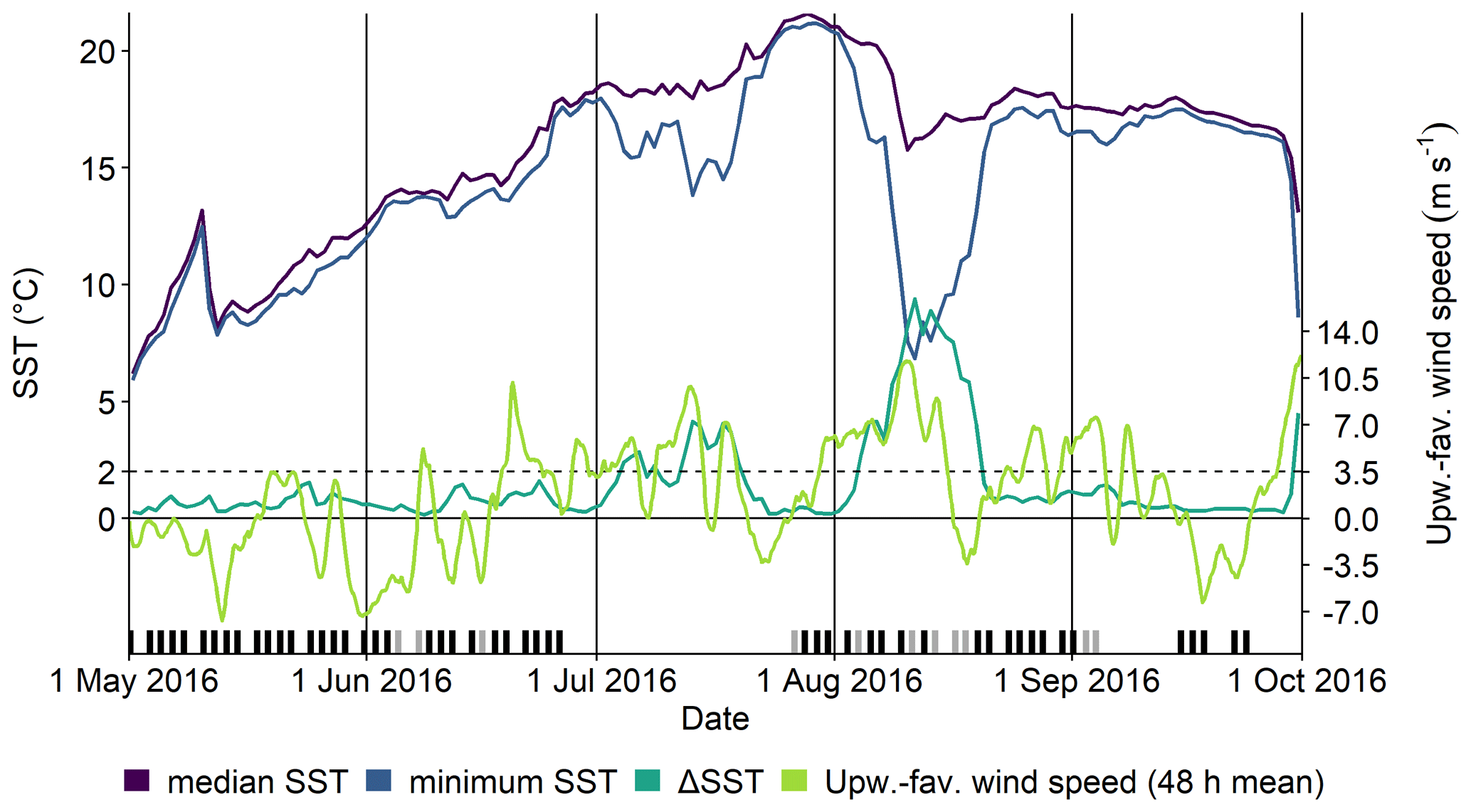
Figure 4 Time series to demonstrate upwelling detection within the Go-SE box. Purple and blue lines are median and minimum model SST along the transect of SOOP Finnmaid; the turquoise line shows their difference (ΔSST). The green line represents the running mean of upwelling-favourable wind speeds, calculated every 3 h for the last 48 h, respectively. The dashed black line indicates the chosen thresholds of the ΔSST and wind criteria, respectively (2 ^∘C, 3.5 m s⁻¹). Each passage of SOOP Finnmaid through the box is marked with a black dash at the bottom. Grey dashes mark when the ship took the western route around Gotland, thereby missing this particular box on the east side. A strong upwelling event in August is observed with small data gaps due to SOOP Finnmaid taking the western route. Another event in July is missed because of a sensor malfunction.

We calculated the wind criterion as a running mean of upwelling-favourable wind speeds of the last 48 h with a temporal resolution of 3 h. The criterion is considered to be “met” if at least four of the eight mean values per day exceed the threshold of 3.5 m s⁻¹.

The ΔSST criterion was calculated as the difference between median and minimum model SST in the respective area since a local upwelling event will lower the minimum SST, while the median remains relatively stable. To achieve a more robust median, the boxes were selected to extend beyond the actual upwelling areas. This results in a pronounced increase in ΔSST during upwelling events, while the criterion is mostly below the 2 ^∘C threshold otherwise. This calculation can be based first on the entire area inside the boxes (Fig. A3) or second on just the sub-transects, i.e along the track of SOOP Finnmaid (Fig. 4). We mainly used the latter for the purposes of this study, which is justified by a comparison of the capability of both approaches to match a daily ΔSST criterion calculated from SST observations aboard SOOP Finnmaid: the second approach based on sub-transects is less sensitive (hit rate: 0.57 vs. 0.94 for the first approach) but has a higher specificity (false alarm rate: 0.08 vs. 0.48) and better skill to forecast correctly (proportion correct: 0.88 vs. 0.57; critical success index: 0.36 vs. 0.21). These verification measures were calculated according to Jolliffe and Stephenson (2003). The differences in number of events correctly identified depending on which subset of SST data is used are explained by the fact that upwelling events start near the coast and then propagate seawards, and thus SST drops along the sub-transect are delayed and often smaller. The first approach (using all SST data within the upwelling box) does not incorporate this lag but is usually better aligned with the wind criterion for the same reason. Therefore, the appropriate method choice depends on the desired use: including more spatial coverage of SST data would be appropriate to analyse the occurrence of upwelling in a certain region statistically. However, we chose to use only SST data along the SOOP route to amplify the agreement with the in situ SST and trace gas measurements. We provide a more detailed method assessment in Sect. 3.1.

Note that a large-scale upwelling event triggers a drop in median SST, but due to increased spatial variability during those events, the sensitivity of ΔSST is usually still sufficient to exceed the threshold of 2 ^∘C in these cases (e.g. Figs. 4 and A3 on ca. 10 August 2016).

3 Results and discussion

3.1 Upwelling statistics based on wind and modelled SST data

To assess the prevalence of upwelling in the data set of SOOP Finnmaid, we identified the main upwelling periods and areas along the transect using the method of combining a ΔSST and a wind criterion (Sect. 2.3). Here, we present a summary of the climatological mean number of days per month and box where the criteria were met (Fig. 5). The ΔSST criterion was calculated based on sub-transects. We provide a full overview further distinguishing by year and selection of SST data (entire box vs. sub-transect) in the Appendix (Figs. B1, B2, and B3). The wind criterion is usually met more frequently than the ΔSST criterion calculated along sub-transects. This reflects that not every occurrence of wind strong enough to induce upwelling leads to upwelled water masses actually reaching the track of SOOP Finnmaid. This is illustrated in Fig. 4 (June 2016) and Animation S1. Downwelling may also lead to quickly vanishing signals (Sect. 3.3). In general, the ΔSST criterion is not very sensitive in May due to a less pronounced thermocline compared to summer. Similarly, only small upwelling-induced trace gas signals are observed in May, which become greater in late summer owing to longer decoupling of surface water and underlying sub-thermocline waters (Sect. 3.4). Upwelling in autumn and winter either leads to a general deepening of the mixed-layer depth (discussed in Gülzow et al., 2013) or plays no important role when the physical and biogeochemical differences between surface and upwelled waters have vanished in winter.

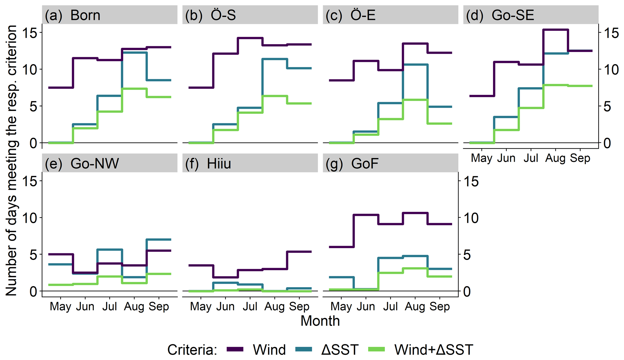
Figure 5 Overview of the two upwelling criteria used in this study: wind (purple) and ΔSST (blue). Displayed is the number of days per month and box in which the respective criterion is met, averaged over 2010 to 2017. ΔSST was calculated along the route of SOOP Finnmaid through the boxes (Sect. 2.3; second approach) to display events that are actually observable from the ship. “Wind+ΔSST” (green) only applies to instances of both criteria being met on the exact same day and therefore excludes occasional instances of lag between wind and ΔSST signals. The openGo box is not included here since no upwelling-favourable wind direction can be defined.

The ΔSST criterion based on the entire area is more sensitive than that calculated along sub-transects but less specific regarding the prediction of upwelling in dynamic areas like the GoF since it is essentially a measure for SST variability>2 ^∘C within the box (Sect. 2.3). It is triggered more frequently than the wind criterion, and due to the high sensitivity of ΔSST, the agreement with the wind criterion – thus both criteria being met – is high (Fig. B3).

The Born, Ö-S, Ö-E, Go-SE, and GoF boxes follow similar patterns with respect to both criteria (Fig. 5), which is not surprising given the fact that in all of these cases, upwelling is induced by the same south-westerly to westerly winds, and the minimum distances to the coast are rather similar. The upwelling-favourable wind direction is opposite in the Go-NW and Hiiu boxes. In the Hiiu box, however, both criteria are almost never met at the same time, which indicates that the distance between sub-transect and coast is too large to observe strong upwelling signals (minimum of 27 km, median of 43 km; Table 1). Admittedly, the sub-transect in the Ö-S box is comparable to Hiiu in terms of distance to the coast, but the crucial difference seems to be the upwelling-favourable wind direction since strong westerly winds are more frequent and intense. This is supported by the fact that, even if we calculate ΔSST based on the entire area, the number of days where both criteria are met in the Ö-S box is higher than in the Hiiu box (Fig. B3), clearly indicating that upwelling is more common in Ö-S. In contrast, the sub-transect in the Go-NW box is frequently influenced by upwelling, but yet, it is the only box where the ΔSST is met more often than the wind criterion (Fig. 5e). We attribute this to the small distance to the coast (minimum of 4 km, median of 10 km; Table 1) leading to higher SST variability and thus more similarity to the ΔSST criterion that includes the entire area (Fig. B3e).

Based on this statistical analysis, we chose the Ö-S box as an example area for most of the following discussion since it features prominent upwelling signals concerning both frequency and magnitude. Additionally, data coverage in this area is high as it is crossed by SOOP Finnmaid on either of its routes (Fig. 1).

3.2 Regional comparison of upwelling events

In this section, we investigate upwelling events that were caused by strong winds across the entire study area in August 2016, leading to temperature and trace gas signals in almost all previously defined upwelling areas (Figs. B1 and B2), which allows us to compare the observations in these regions and to assess the importance of upwelling for the observed trace gas dynamics. This case study exemplifies more general findings we gained during the analysis of the entire data set.

The entire month was characterised by strong westerly to south-westerly winds (Fig. 4), leading to upwelling in the Born, Ö-S, Ö-E, Go-SE, and GoF boxes, interrupted by a week (15–22 August 2016) of more north-easterly winds, triggering upwelling in the Hiiu and Go-NW boxes. The resulting SST drops by up to 16 ^∘C predominantly near all southern and eastern coasts propagated seawards and relaxed within several weeks (Animation S1). Coverage of data from SOOP Finnmaid in this period is very dense, with the majority of transects along the east side of Gotland (see ratio of black and grey dashes in Fig. 4). We illustrate the temporal and spatial evolution of this event (Fig. 6) taking the example of the Ö-S box.

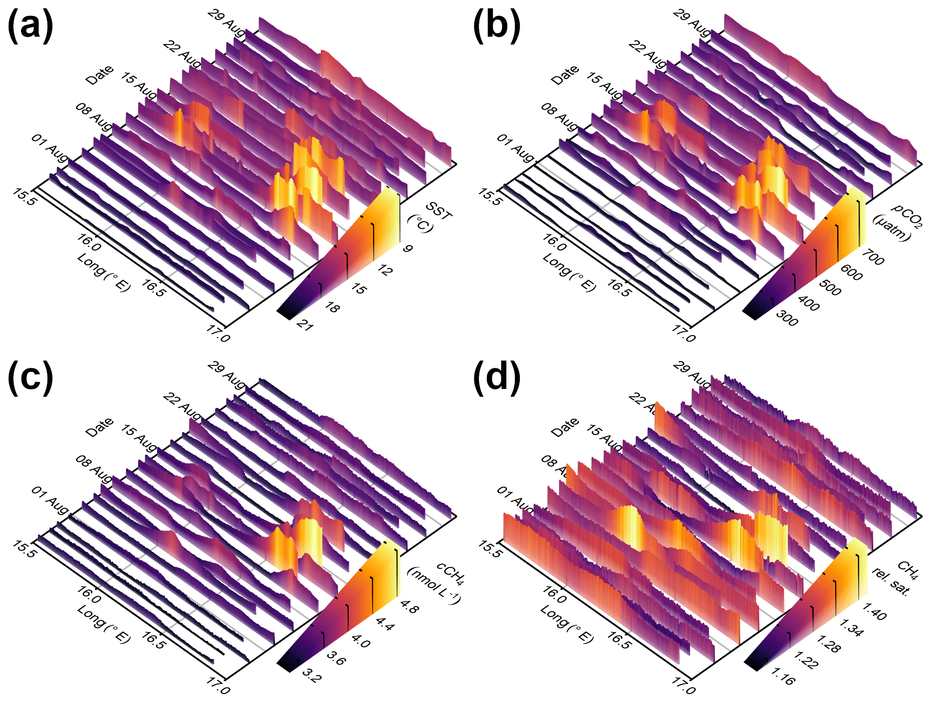
Figure 6 (a) Sea surface temperature, (b) CO₂ partial pressure, (c) CH₄ concentration, and (d) relative CH₄ saturation within the Ö-S box as measured by SOOP Finnmaid on 21 sub-transects from 26 July to 30 August 2016. In all panels, abscissa is position given as longitude, ordinate is time, and the respective variable is displayed by both colour and height of the curve. Please note the inverted SST scale in (a) to highlight the correlation between decreasing SST and increasing pCO₂ and cCH₄. Data presented in (a–c) correspond to Fig. 7b and j.

Before the event, SST is at a typical summer value of 21 ^∘C throughout the entire sub-transect. As expected, upwelling leads to SST decreases (displayed as peaks in Fig. 6a) with temperatures down to 9 ^∘C. These minima move over time (see also Animation S1) and are subject to relaxation, which is further discussed in Sect. 3.3. The pre-upwelling temperature is usually not reached again during this time of the year, most probably due to an increased mixed-layer depth as an additional effect of stronger winds and weakened solar irradiation at the end of August.

The observed trace gas patterns are similar to the temperature distribution: the first sub-transect can be considered to be background conditions with typical late summer values of about 250 µatm for pCO₂ and 3.2 nmol L⁻¹ for cCH₄ in this area. During the upwelling event, we observe elevated pCO₂ and cCH₄, with trace gas maxima correlated to minimum SST. For CO₂, this results in a switch from undersaturation to supersaturation. CH₄ is always supersaturated or in equilibrium with the atmosphere in the SOOP Finnmaid data set, and strong upwelling further increases this supersaturation and, eventually, CH₄ outgassing. However, upwelling is not the only factor controlling increased CH₄ supersaturation (Fig. 6d). Warming of upwelled waters increases pCH₄ and, therefore, relative saturation. As with SST, the enhanced trace gas levels relax subsequentially.

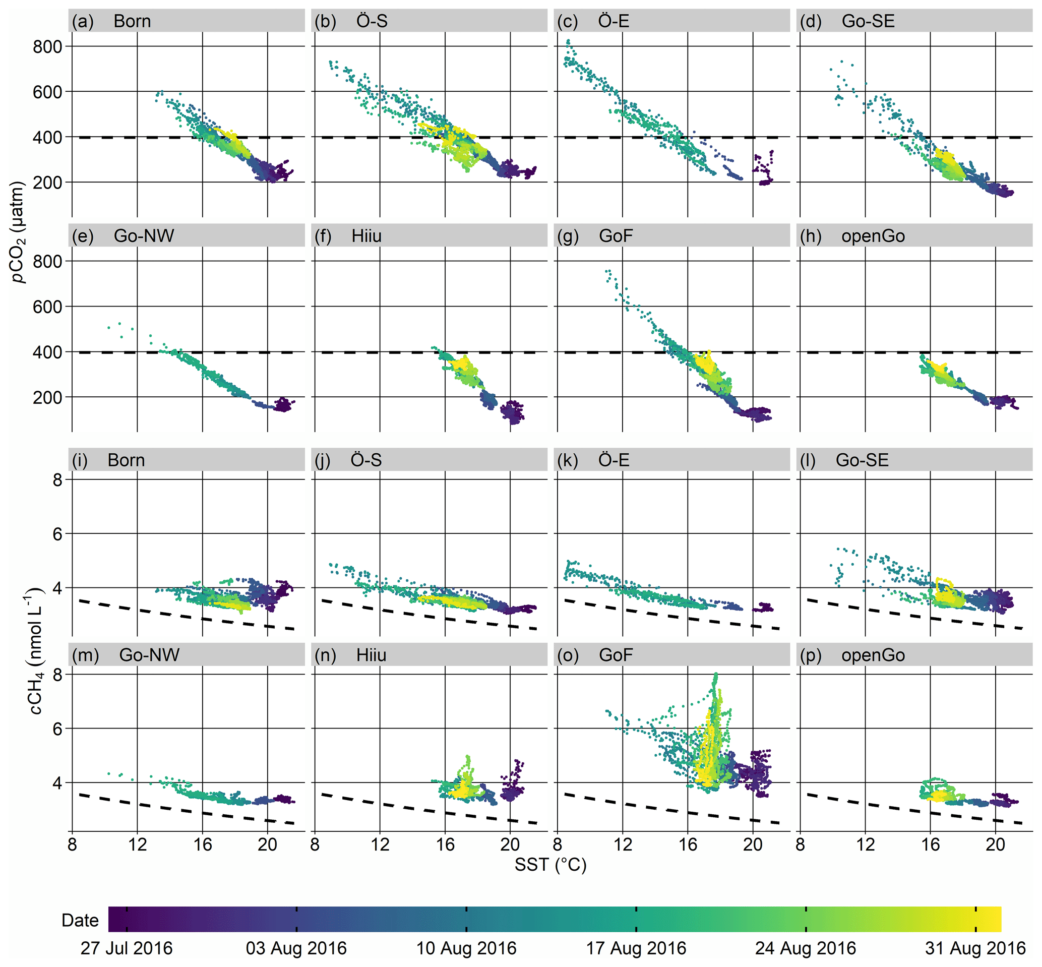
Figure 7 Surface pCO₂ (a–h) and cCH₄ (i–p) as measured by SOOP Finnmaid on 21 transects from 26 July to 30 August 2016, each plotted against SST within the seven upwelling regions and the open Gotland Sea box for comparison. The measurement date is colour-coded. Temporal coverage in the Go-SE box (15 transects; see black dashes in Fig. 4) and the Ö-E and Go-NW boxes (6 transects; see grey dashes therein) is reduced since SOOP Finnmaid uses two different routes around Gotland. Dashed black lines indicate atmospheric-equilibrium partial pressure for CO₂ and concentration for CH₄ (calculated using mean salinity per box in the given time period), respectively.

To extend these findings to the different regions, we investigated the relationships between trace gas data and temperature over time (Fig. 7). The example from the Ö-S box is representative of the majority of strong upwelling events affecting trace gases in the data set of SOOP Finnmaid, which are generally characterised by near-linear relationships between trace gases and SST. Maximum pCO₂ and cCH₄ values would not be reached without upwelling in summer (Fig. B4). We observe the same behaviour in the Go-SE, Ö-E, and Go-NW boxes despite their reduced data coverage (Fig. 7). The Ö-E box features the highest pCO₂ in the data set of over 800 µatm. In the Go-NW box, the observable upwelling event began only at the end of trace gas data coverage on the western route due to a different favourable wind direction; hence, the more extreme values are missing in this example. However, the resulting pattern resembles the ones of the Ö-S, Ö-E, and Go-SE boxes, just with lower maximum pCO₂ and cCH₄.

The Born and GoF boxes show the same relationships as the previous boxes in their pCO₂–SST diagram, with considerable dynamic range in the case of the GoF box (Fig. 7a and g). The respective cCH₄–SST diagrams, however, only contain a small branch of increasing cCH₄ with decreasing SST (Fig. 7i and o). These regions are dominated by temperature-independent CH₄ variability, which indicates that other processes than upwelling might cause higher-than-usual cCH₄: the Born box is situated between two basins (Arkona and Bornholm basins), which are interlinked via lateral transport and which both feature gassy sediments (Gülzow et al., 2014; Tóth et al., 2014), from which CH₄ may be released via pressure changes caused by strong winds (Schneider von Deimling et al., 2010; Gülzow et al., 2013); cCH₄ variability in the GoF box might be driven by the highly variable physical conditions, e.g. changes in the estuarine circulation up to full reversal (Westerlund et al., 2019) or enhanced vertical transport by boundary wall shear (Schmale et al., 2010). These effects would lead to a less distinct impact of upwelling compared to the Ö-S, Ö-E, Go-SE, and Go-NW boxes, where vertical decoupling is more stable.

The discussed phenomena can be contrasted with the behaviour of the sub-transect within the Hiiu box: although we find a clear correlation between decreasing SST and increasing pCO₂ resembling that of the other boxes, we do not observe temperatures lower than 15 ^∘C and pCO₂ higher than 420 µatm, which is close to atmospheric equilibrium (Fig. 7f). This relationship is similar to that of the openGo box, the patterns in which we attribute to mixed-layer deepening and air–sea gas exchange caused by stronger winds instead of upwelling because of its distance to the coast (minimum of 40 km, median of 64 km; Table 1). Since the route of SOOP Finnmaid within the Hiiu box is the farthest away from the coast of all boxes (minimum of 27 km; median of 43 km; Table 1), and the observed pCO₂–SST relationships are so similar to openGo, we infer that upwelling has only minor influence on the observed values in this region during this time period. This is consistent with maps of modelled SST (Fig. 3 and Animation S1; most pronounced around 18 August 2016), where no upwelled water masses reach out to the ship track, and confirms the same finding from the statistical identification of main upwelling areas presented in Sect. 3.1.

The cCH₄–SST diagram of the Hiiu box (Fig. 7n) resembles, to some extent, that of the GoF box (Fig. 7o) without the upwelling branch and smaller maximum cCH₄ and indicates considerable cCH₄ variability compared to, for example, the Ö-S, Ö-E, Go-SE, and Go-NW boxes. In late July, for example, CH₄ concentration drops from 4.8 to 3.3 nmol L⁻¹ at more or less constant temperature (Fig. 7n), equating to a change in relative CH₄ saturation from 1.9 to 1.3. In the adjacent region of openGo, no instances of increasing cCH₄ at constant SST (vertical branches in Fig. 7n–p) were observed.

We summarise that upwelling affects observed SST, pCO₂, and cCH₄ drastically in the defined boxes in late summer of 2016. It typically causes near-linear relationships between surface trace gas signals and temperature with varying ranges and slopes between regions. For CO₂, this can be observed in all regions (with limitations in the Hiiu box), while in the case of CH₄, strong variability caused by other processes may mask the effects of upwelling, and closest-to-linear relationships are observed in the Ö-S, Ö-E, Go-SE, and Go-NW boxes.

3.3 Typical relaxation of upwelling-induced trace gas signals

The surface water properties of a region influenced by upwelling change over the course of the upwelling event. This can be seen in Fig. 7, where the evolution of the relationship over time between SST and pCO₂ or cCH₄ is indicated by colour, and in Fig. B4. Before an event, we observe high temperature and low trace gas levels, with low spatial variability within sub-transects. During strong upwelling, a larger variability in SST, pCO₂, and cCH₄ is observed concurrently as SOOP Finnmaid transects the respective region. Trace gas and SST data are usually related linearly after the upwelling event. After upwelling-favourable winds cease, the range of signals as well as their intensity is reduced through relaxation in a quasi-linear fashion (Fig. 7). The final state after relaxation, when compared to the initial state, is shifted towards lower temperatures; higher pCO₂; and slightly elevated cCH₄, which equals a roughly comparable CH₄ supersaturation at this decreased, final temperature. Depending on the time of the year, SST might re-increase due to subsequent warming or not recover completely (as in late summer).

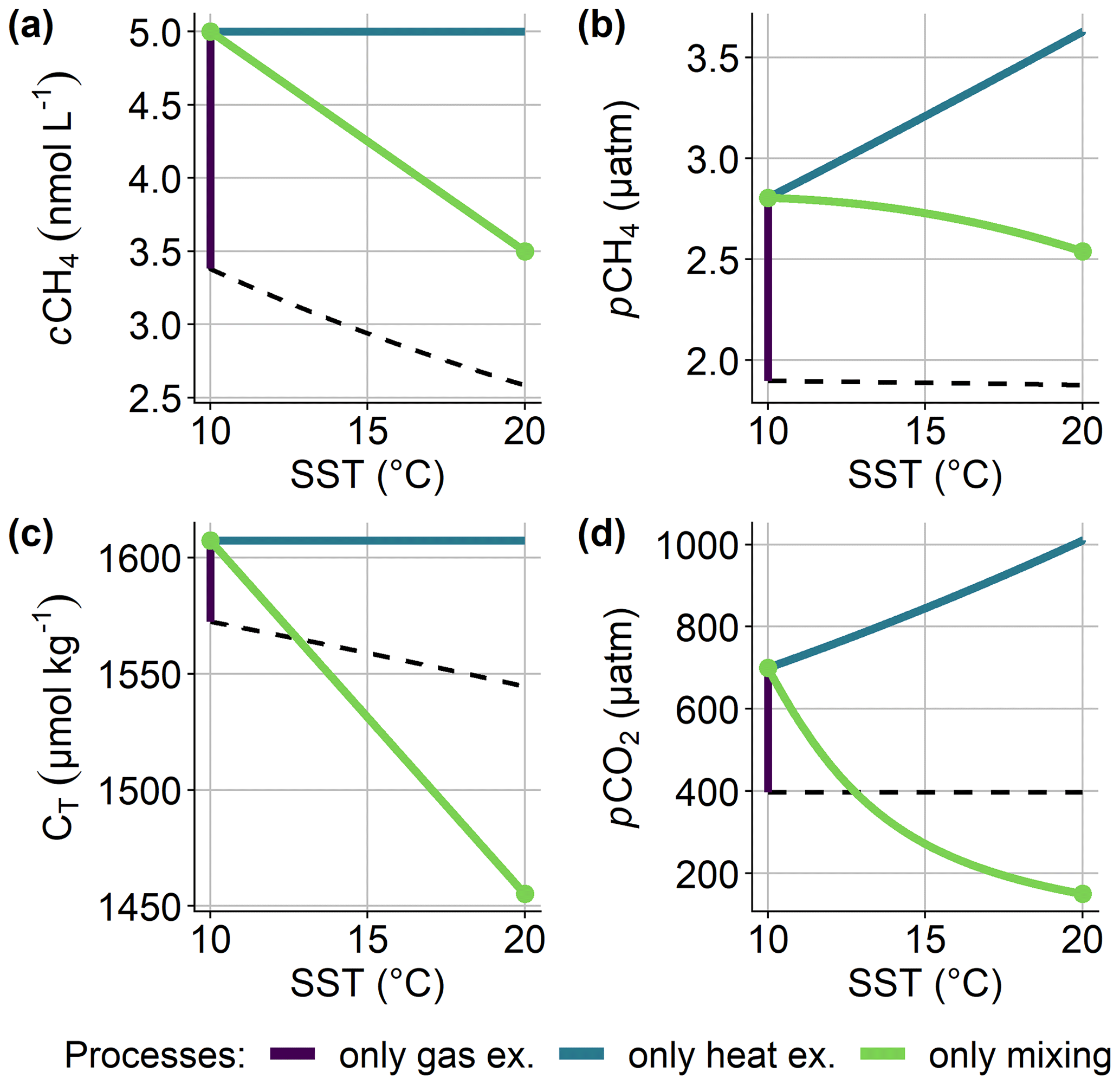
Figure 8 Theoretical relaxation curves of surface trace gas and temperature signals caused by upwelling. We calculated all graphs based on the processes (i) air–sea gas exchange, (ii) air–sea heat exchange, and (iii) mixing with a typical water mass with pre-upwelling conditions, with only one process considered at a time, starting at the point where the three lines intersect. Bold green points highlight the mixing endmembers. Dashed black lines indicate atmospheric-equilibrium conditions for the respective trace gas (397 ppm of CO₂, 1920 ppb of CH₄). Mixing lines were calculated for (a) cCH₄ using linear interpolation between endmembers (conservative behaviour), (b) pCH₄ from cCH₄ and SST, (c) C_T using linear interpolation between endmembers whose C_T was calculated from A_T and pCO₂ (conservative behaviour), and (d) pCO₂ from C_T and A_T. See Sect. B1 for details concerning calculation parameters.

In order to discuss the processes that are involved in the relaxation of upwelling signals, we calculated theoretical relaxation curves in trace gas–temperature diagrams (Fig. 8). Assumed endmember characteristics, physical driving parameters, and process descriptions are summarised in Sect. B1. We focus on air–sea gas exchange, air–sea heat exchange, and mixing with a typical water mass with pre-upwelling conditions. CH₄ oxidation in the upper, oxic water column should not play a major role on the short timescales considered here (Jakobs et al., 2013). Primary production (e.g. by nitrogen fixation) has the potential to decrease pCO₂ distinctly but is difficult to constrain since it depends on meteorological conditions and nutrient availability with possible time lags of several weeks (Vahtera et al., 2005; Wasmund et al., 2012).

The relaxation of SST is mainly driven by mixing. We estimated a total surface heat flux of ca. 300 $\mathrm{J}{\mathrm{m}}^{-\mathrm{2}}{\mathrm{s}}^{-\mathrm{1}}$, which translates to a daily SST change of ca. 0.4 K d⁻¹ assuming a mixed-layer depth of 15 m, which is rather typical for windy conditions in summer (derived from model data, not shown). Therefore, air–sea heat exchange contributes only little to the observed warming of upwelled water masses on the order of 5–10 K, leaving mixing as the dominant process. Despite the excess of the surrounding water masses, mixing does not necessarily lead to pre-upwelling conditions since the endmember may change due to enhanced mixing in the open basins caused by stronger wind. SST might re-increase in the following weeks depending on meteorological conditions.

Mixing also shapes the typically observed cCH₄–SST relationships (Figs. 7i–o and 8a), leading to near-linear mixing curves since concentration is a conservative parameter with respect to temperature changes (we neglect the influence on water density here). The upwelled water mass releases ca. 7700 $\mathrm{nmol}{\mathrm{m}}^{-\mathrm{2}}{\mathrm{d}}^{-\mathrm{1}}$ of CH₄ into the atmosphere. This results in a daily cCH₄ loss of 0.51 $\mathrm{nmol}{\mathrm{L}}^{-\mathrm{1}}{\mathrm{d}}^{-\mathrm{1}}$ in a 15 m mixed layer, which is an efficient sink considering the magnitude of observed concentrations. Therefore, air–sea gas exchange alters the slope of the cCH₄–SST relationship. Note, however, that gas flux is highly dependent on wind speeds, which are biased in cCH₄–SST diagrams presented here: pre-upwelling conditions involve low wind speeds, while the upwelling event is caused by stronger winds, which eventually weaken. Heat exchange has no influence on cCH₄, but the relative CH₄ saturation is determined by its partial pressure pCH₄, which increases by the order of 2 % K⁻¹ (Wiesenburg and Guinasso, 1979). This effect should not play a major role concerning relaxation given the low surface heat flux. However, as outlined above, SST might re-increase in the following weeks, thereby increasing pCH₄, and thus potentially lead to enhanced fluxes into the atmosphere over a longer time period of weeks following the upwelling event. Likewise, mixing leads to elevated pCH₄ and relative saturation compared to linear behaviour (Fig. 8b).

Similarly, the relaxation of pCO₂ cannot be considered independently from SST relaxation due to its temperature dependence. Warming by air–sea heat exchange causes a pCO₂ increase on the order of 4 % K⁻¹ (Takahashi et al., 1993), which should not play a major role concerning relaxation given the low surface heat flux. As with pCH₄, however, this effect could lead to increasing pCO₂ and enhanced CO₂ fluxes into the atmosphere (or reduced fluxes into the sea) in the following weeks.

The relaxation of upwelling-induced pCO₂ signals (Fig. 7a–g) cannot be explained solely by mixing because the theoretical pCO₂–SST mixing curve obtained from CO₂ system calculations features a distinct curvature with lower pCO₂ compared to linear behaviour (Fig. 8d). The observed near-linear relationship is likely caused by air–sea CO₂ exchange: at a wind speed of 10 m s⁻¹, the upwelled water mass in this example (Fig. 8d) releases ca. 0.074 $\mathrm{mol}{\mathrm{m}}^{-\mathrm{2}}{\mathrm{d}}^{-\mathrm{1}}$ of CO₂ into the atmosphere, which translates into a daily C_T (total dissolved inorganic carbon) loss of 4.8 $\mathrm{\mu }\mathrm{mol}{\mathrm{kg}}^{-\mathrm{1}}{\mathrm{d}}^{-\mathrm{1}}$ in a 15 m mixed layer. This C_T decrease in CO₂-oversaturated waters explains the deviation from the expected linear (conservative) mixing curve in C_T estimated from pCO₂ observations (Fig. B5 vs. Fig. 8c). Primary production triggered by upwelling has a similar (potentially even greater) influence on pCO₂ but with different kinetics. One could argue that air–sea CO₂ exchange should similarly increase C_T in CO₂-undersaturated waters, which is not observed (Fig. B5). This can be explained with the aforementioned wind speed bias, resulting in very low fluxes under pre-upwelling conditions (see also Sect. 3.5). The bent C_T–SST curve translates into a near-linear pCO₂–SST curve, which, in conclusion, can be interpreted as the combined result of mixing and decrease in the highest pCO₂ values due to gas exchange and possibly primary production.

The importance of air–sea gas exchange as a relaxation process and the potential long-term effect of increasing supersaturation due to heat exchange imply that upwelling amplifies surface trace gas fluxes, especially for CH₄, by circumventing the sink of CH₄ oxidation in the water column. Schneider et al. (2014b) mentioned these upwelling-induced trace gas fluxes previously for the Baltic Sea but questioned the importance for the annual balance since the upper water column would be ventilated in autumn and winter anyhow, and CH₄ turnover times in the upper, oxic water column are on the magnitude of years (Jakobs et al., 2013). Despite a more detailed analysis of the statistical prevalence of upwelling in this study, the question of the importance of upwelling in the annual trace gas balance of the Baltic Sea cannot be answered here based on the data available. Apart from the high variability within observed upwelling events, general statements on this matter are further complicated by little knowledge about fluxes in shallow areas (Humborg et al., 2019), large heterogeneities between basins (Gülzow et al., 2013), and the unknown CO₂ source and sink behaviour of the entire Baltic Sea (Schneider et al., 2014b). Answering this question in the future requires more knowledge of the Baltic Sea CO₂ and CH₄ balances in general and extended insight into limitations of upwelling-induced flux estimates in the Baltic Sea (discussed in Sect. 3.5).

Another possible relaxation pathway is downwelling. Figure B6 provides an example of quickly vanishing upwelling signals after turning wind. There, we expect downwelling to quickly remove upwelled waters from the surface, thereby restoring the previous surface water mass that underwent only small changes in SST, pCO₂, and cCH₄. This limits enhanced trace gas fluxes to a short time period during the upwelling event. This example is rather unique because it requires upwelling- and downwelling-favourable wind conditions in quick succession and can only be observed in close proximity to the coast (the Go-NW box in this example), i.e. where the upwelled water mass is young and has not yet expanded towards the open sea. We can exclude lateral transport out of the box as a possible explanation for this effect based on maps of modelled SST (data not shown).

3.4 Interannual variability in upwelling-induced trace gas signals

Since upwelling in the Baltic Sea is an episodic phenomenon based on wind conditions, it is subject to considerable interannual variability. In Fig. 9, we present seasonal plots (from May to September) of pCO₂ and cCH₄ versus SST in the Ö-S box. The coloured date scale allows the temporal evolution of signals to be followed throughout the season and also highlights larger data gaps (e.g. in 2012 and 2013).

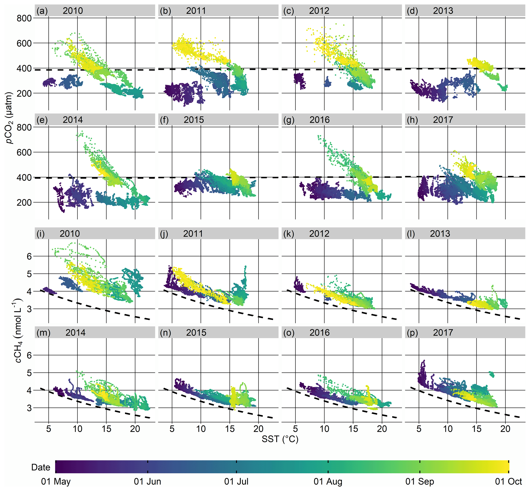
Figure 9 Surface CO₂ partial pressure (a–h) and CH₄ concentration (i–p) from 1 May to 30 September within the Ö-S box, each plotted against temperature for individual years. The measurement date is colour-coded. Dashed black lines indicate atmospheric-equilibrium partial pressure and concentration (calculated using mean seasonal salinity), respectively.

Most years feature consistent patterns with respect to pCO₂ (Fig. 9), reflecting its yearly cycle (see Introduction and Schneider and Müller, 2018): CO₂ is already undersaturated with respect to the atmosphere in May due to primary production during the spring bloom. Over the following weeks, the change in pCO₂ is usually rather small, but SST increases as a result of solar irradiation and often weaker winds (see also Fig. B4). The resulting stabilisation of the surface thermocline and the accumulation of remineralised CO₂ below combined with decreasing air–sea CO₂ exchange and ongoing primary production lead to increasing pCO₂ gradients between surface and sub-thermocline water (which are the cause of upwelling-induced pCO₂ signals; Fig. 2) and a permanent undersaturation of the surface water with respect to the atmosphere. The characteristic cCH₄–SST conditions follow the CH₄ equilibrium curve towards lower concentrations at higher temperatures most probably due to air–sea CH₄ exchange, maintaining a persistent supersaturation. In most years, most notably in 2010, 2012, 2014, and 2016, strong upwelling around August overrides these typical summer conditions, resulting in characteristic pCO₂–SST and cCH₄–SST patterns. For these years, the ranges of SST, pCO₂, and to a certain extent cCH₄ are similar (but still not equal), with the notable exception of very dynamic cCH₄ in 2010. For the other years, we observe a high degree of variability from these typical conditions: strong upwelling-favourable winds in June 2011 led to an early increase in pCO₂ and lower SST overall. Later, at the end of July 2011, a pronounced, sharp increase in cCH₄ at a rather constant temperature was observed, which clearly is not related to upwelling.

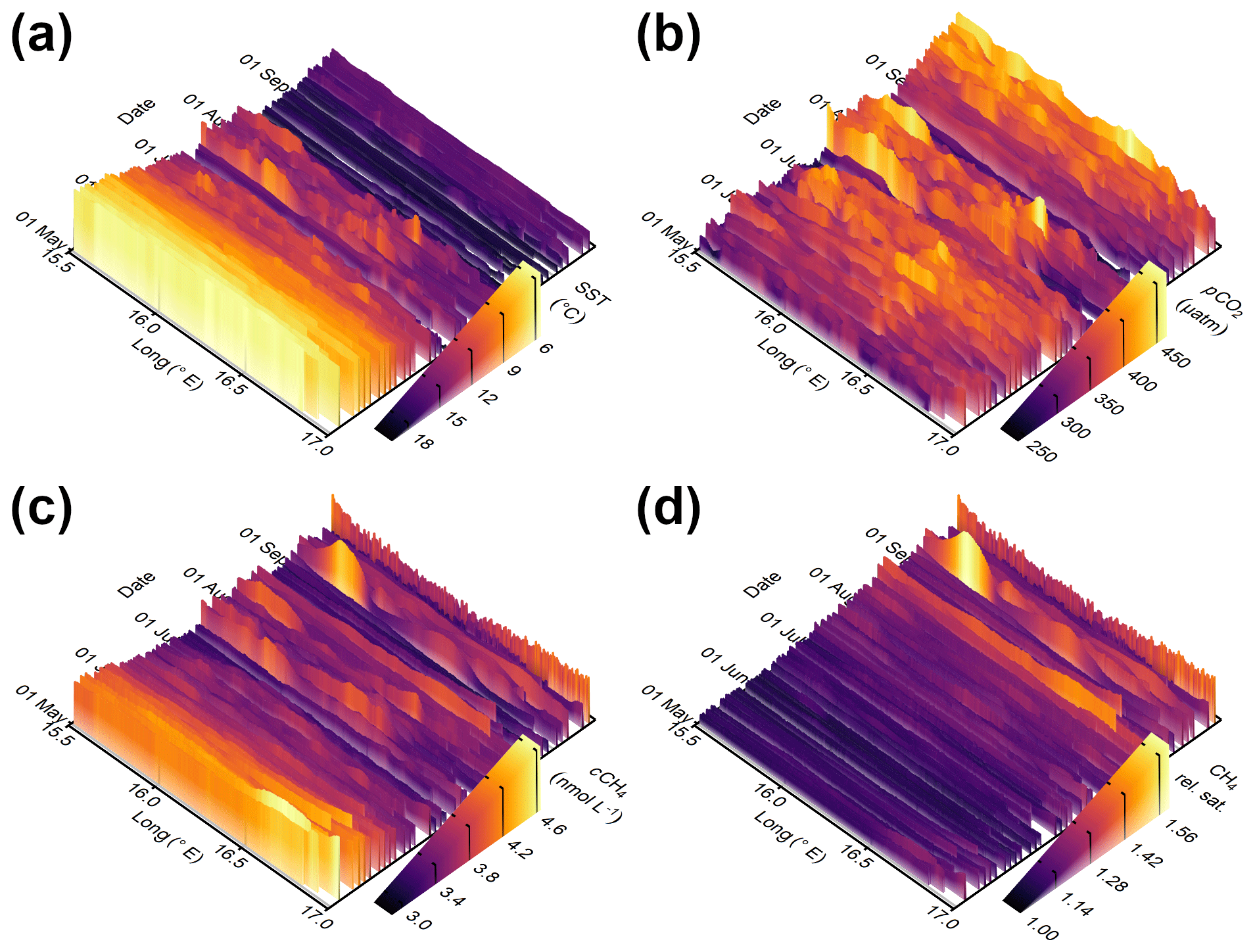
Figure 10 (a) Sea surface temperature, (b) CO₂ partial pressure, (c) CH₄ concentration, and (d) relative CH₄ saturation within the Ö-S box on 82 transects from 2 May to 21 September 2015. In all panels, abscissa is position given as longitude, ordinate is time, and the respective variable is displayed by both colour and height of the curve. Please note the inverted SST scale in (a) to highlight the correlation between decreasing SST and increasing cCH₄ and pCO₂. Data presented in (a–c) correspond to Fig. 9f and n.

The year 2015 is particularly interesting because it demonstrates the influence of quasi-continuous upwelling-favourable winds over the course of several months, which overrides the typical summer trace gas situation. The year was dominated by upwelling-favourable, westerly winds until the beginning of August (Fig. A4), effectively prohibiting strong thermal stratification of the surface water (Fig. 10a and low maximum temperature in Fig. 9f and n). This special case is problematic for the detection method because the observable ΔSST gradients become too small for every day to be counted as an “upwelling day” (Fig. A4). As a result of weakened stratification, surface CO₂ undersaturation is unusually weak compared to the typical summer situation (Fig. 10b and high minimum pCO₂ in Fig. 9f). Furthermore, we observe reduced cCH₄ variability as a result of continuous mixing and intensified air–sea exchange through increased turbulence so that cCH₄ follows the equilibrium curve more closely than during most years (Fig. 9n). Elevated cCH₄ (Fig. 10c) does not necessarily translate into elevated saturation (Fig. 10d) depending on SST; however, as pointed out in Sect. 3.3, the water mass will become supersaturated as a consequence of subsequent warming. In July 2015 (turquoise hues in Fig. 9f and n), near-linear trace gas–temperature curves are characteristic for strong upwelling (see Sect. 3.2). Compared to, for example, August 2014 and 2016, however, where the upwelling SST, pCO₂, and cCH₄ signals stand out prominently from the rest of the values, their range concerning all three parameters is reduced in 2015 since decoupling of surface and underlying water was partly impeded.

It was not possible to identify trends in frequency or magnitude of enhanced pCO₂ and cCH₄ caused by upwelling events on the limited timescale of 8 years covered by our observations. The main reason for this is the high spatial and temporal variability in upwelling (and of several other processes with influence on dissolved trace gases) in the Baltic Sea, which led to the necessity to do parts of the analyses on a per-event basis and effectively impeded a universal approach. Moreover, the observed endmembers of minimum SST and maximum pCO₂ and cCH₄ are dependent on data coverage, which adds another layer of uncertainty to any trend analysis on the data set, especially in boxes around Gotland (two different ship routes) and during years with larger data gaps. Typical water residence times of 10–30 years (Feistel et al., 2010) imply that longer trace gas time series are needed to detect not only variability but also trends using the methods we presented here. In fact, Schneider and Müller (2018) managed to find a trend in surface pCO₂ between 4.6 and 6.1 µatm yr⁻¹ in the Baltic Sea from 2008 to 2015 but did so without a focus on upwelling events only and by filling data gaps through interpolation, which effectively yielded a considerably larger data basis compared to this study. We suppose that if, at some point, the extrapolation scheme proposed in Sect. 3.5 could be expanded to cover more than single events, a trend analysis based on the resulting pCO₂ and cCH₄ fields should be possible since these data would not be restricted by spatio-temporal coverage or event-specific features.

3.5 Potential to estimate upwelling-induced air–sea trace gas fluxes

The observed near-linear relationships between pCO₂ or cCH₄ and SST can be used to spatially extrapolate trace gas observations from sub-transects based on modelled SST fields, assuming that these relationships are consistent for entire upwelling areas. This enables us to estimate air–sea CO₂ and CH₄ fluxes resulting from upwelling events (Fig. 11, Sect. B1). Since we used linear regression (Fig. 11f and g), SST minima near the coast translate into pCO₂ and cCH₄ maxima, retaining the overall pattern and fine structure of the SST field (Fig. 11a–c).

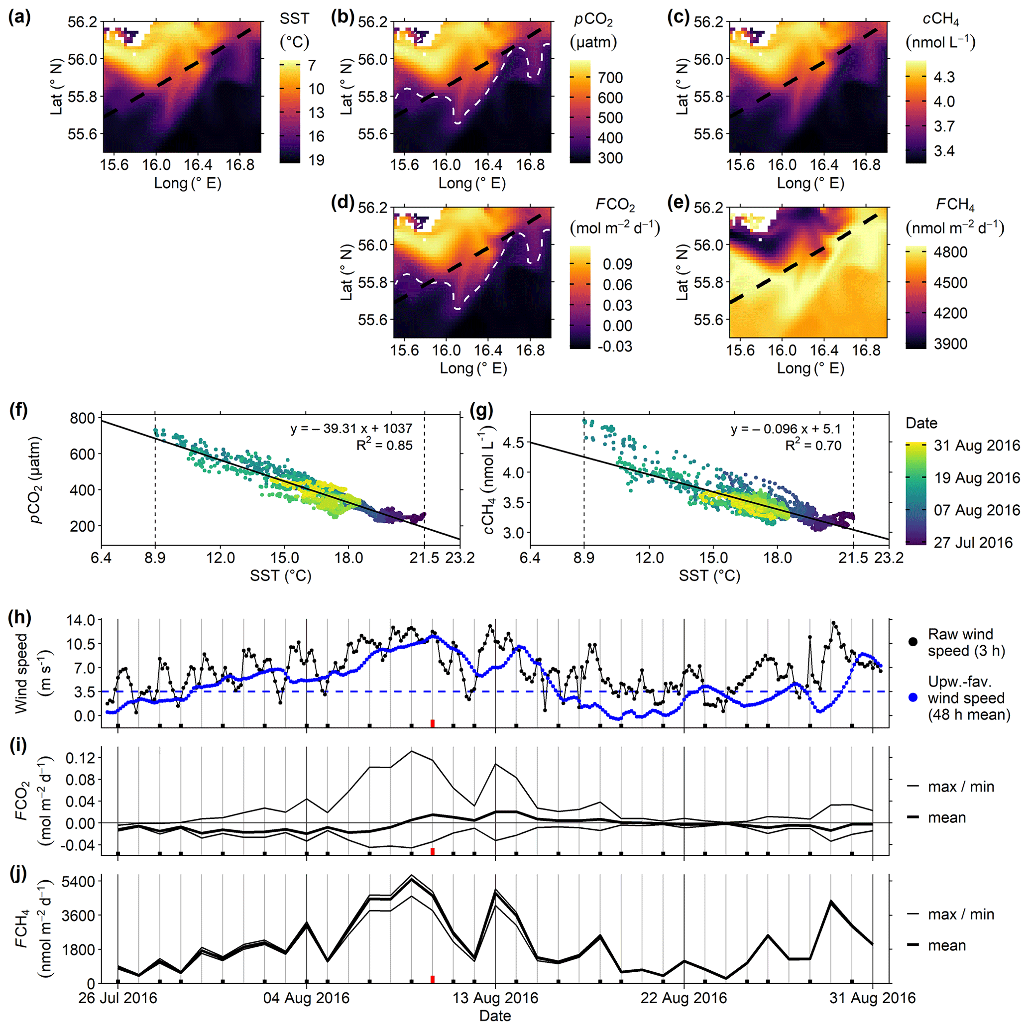
Figure 11 Air–sea trace gas flux estimate for region Ö-S from 26 July to 31 August 2016. Maps depict the situation on 10 August, when SST was minimal: (a) modelled SST (inverted colour scale), based on which (b) pCO₂ and (c) cCH₄ were extrapolated from measurements aboard SOOP Finnmaid, leading to air–sea flux estimates of (d) CO₂ and (e) CH₄. Dashed black lines represent the track of SOOP Finnmaid; dashed white lines indicate atmospheric equilibrium for CO₂ (CH₄ is always supersaturated). (f) Relationships of pCO₂ or (g) cCH₄ and SST, which were used for the calculation of pCO₂ and cCH₄ in (b) and (c), as measured by SOOP Finnmaid on 21 sub-transects from 26 July to 30 August 2016, with colour indicating date (same as Fig. 7b and j). Dashed vertical lines display the observed SST range, while the limits of the SST axis represent the range of modelled SST and thus the extrapolation limits. The relationships were approximated via linear regression (solid black line); the regression functions and R² are given in the respective panels. (h) Wind speed (black dots and lines) and the running 48 h mean of upwelling-favourable wind speed (blue dots and lines) over time, with the dashed blue line indicating the threshold of the wind criterion (3.5 m s⁻¹). (i) Daily air–sea CO₂ and (j) CH₄ fluxes over time. Bold lines represent mean and thin lines maximum and minimum fluxes per day, respectively. Black dashes at the bottom of (h–j) mark transects of SOOP Finnmaid within the box; a long red dash marks 10 August, the date of the maps (a–e).

The CO₂ flux (FCO₂; Fig. 11d) depends on the difference in pCO₂ between sea and air, which determines the flux direction, and the transfer coefficient, which is parameterised mostly by wind speed. Therefore, pCO₂ and FCO₂ share the same spatial pattern, with positive and negative fluxes being present in the box at the same time. Both CO₂ outgassing (0.13 $\mathrm{mol}{\mathrm{m}}^{-\mathrm{2}}{\mathrm{d}}^{-\mathrm{1}}$) and uptake (−0.046 $\mathrm{mol}{\mathrm{m}}^{-\mathrm{2}}{\mathrm{d}}^{-\mathrm{1}}$) peak on 9 August, when wind speeds are highest. CH₄ fluxes (FCH₄; Fig. 11e) into the atmosphere reach their maximum (5730 $\mathrm{nmol}{\mathrm{m}}^{-\mathrm{2}}{\mathrm{d}}^{-\mathrm{1}}$) on the same day. However, the spatial distribution of FCH₄ differs from that of cCH₄ due to the temperature dependence of the CH₄ equilibrium concentration: for instance, the lowest fluxes on 10 August occur close to the coast despite high concentrations in this area because supersaturation decreases with lower SST, indicating that the upwelled water mass has a lower CH₄ supersaturation than the surrounding waters in this example. However, relative CH₄ saturation is highly sensitive to changes in slope of the applied regression curve, which underestimates the observed maximum supersaturation in this example (Fig. 11g) and likely leads to this special spatial distribution. Even careful tweaking of the regression curve would result in a pattern much more similar to that of FCO₂, and this similarity increases with increasing supersaturation of the upwelled water mass compared to pre-upwelling conditions. In other examples, the two flux patterns are more similar than here (data not shown). The discussed “tweaking” of the cCH₄–SST regression, though impacting the derived pattern considerably, would have only a small impact on the areal flux. In any case, daily FCH₄ peaks under intermediate conditions where the flux-increasing effects of rising cCH₄ and rising SST combine. On many days in this example, including 10 August (Fig. 11e), this area of maximum daily FCH₄ is in close proximity to the transect of SOOP Finnmaid, where it can be observed by in situ measurements, whereas areas of maximum daily FCO₂ tend to be closer to the coast. It should be noted that the spatial variability in FCO₂ is much higher than that in FCH₄ (see maximum and minimum values in Fig. 11i and j).

The importance of wind is also reflected by the evolution of air–sea gas fluxes over time (Fig. 11i and j). Fluxes are weak under pre-upwelling conditions due to low wind speeds (Fig. 11h); increase distinctly with rising wind speeds; and reach a minimum (considering absolute values for FCO₂) in the relaxation period after the upwelling event, when the wind calms down again. The sea is a permanent source of atmospheric CH₄ with varying strength based mostly on wind speed in this example, which can be generalised to the entire data set. In contrast, FCO₂ is negative (CO₂ uptake from the atmosphere) under pre-upwelling conditions. CO₂ outgassing starts with the onset of upwelling, but at this point, the area is still dominated by increasing CO₂ uptake due to rising wind speeds. Both positive and negative CO₂ fluxes intensify over the following days, but CO₂ outgassing reaches higher absolute values as a result of high pCO₂ due to upwelling. The area is a net source of CO₂ for the atmosphere (mean FCO₂>0) from 9 August, when wind speeds are maximal, to 19 August, when pCO₂ gradients have sufficiently diminished due to relaxation. Note, however, that mean FCO₂ depends on the (arbitrary) choice of box boundaries.

The presented flux estimates depend largely on the applicability of the observed near-linear trace gas–SST relationships for the entire area and period, including extrapolation to temperatures lower than the minimum temperature of the trace gas–SST regression (i.e. towards the core of the upwelled water mass; see SST axis in Fig. 11f and g). Verification of this assumption would require a dedicated research cruise involving trace gas measurements perpendicular to the track of SOOP Finnmaid with transects towards both the coast and open basin. Based on the presented findings, we assume that the extrapolation scheme proposed here leads to a conservative estimate of the actual fluxes since the applied regression is based on waters that have already been subject to air–sea gas exchange (see also Sect. 3.3) as opposed to “young” upwelled waters, which are not observed by SOOP Finnmaid. Still, the presented method provides a means to constrain upwelling-induced trace gas fluxes based on SOOP and model (or, potentially, remote sensing) data on large spatial and temporal scales, which may also be used to study other upwelling areas than the Baltic Sea. We recommend using this approach on a per-event basis to properly calibrate the applied trace gas–SST relationships, which might differ between regions and events. In general, this extrapolation method should be applicable in every upwelling area worldwide where near-linear trace gas–SST relationships are observed and could, therefore, be a valuable tool to produce flux maps from (scarce) surface observations.

4 Conclusions

Upwelling in the Baltic Sea can be observed using autonomous measurements aboard SOOPs, which, compared to dedicated research cruises, provide higher spatial and temporal coverage at the cost of being restricted to surface data and, depending on route, a larger distance to the coast. They enable studies on seasonality, comparison of regions, and observation of processes over long time periods. Combining SOOP-based trace gas measurements with other high-resolution data sets like model or remote sensing data further allows us to (a) assess their spatial and temporal representativity by adding information beyond the ferry track; (b) assess the prevalence of upwelling even during SOOP data gaps caused by ship schedule and (rare) outages; (c) compare events by size, duration, and signal intensity; and (d) estimate upwelling-induced air–sea fluxes.

Based on the long-term SOOP data set, we identified controlling parameters of upwelling-induced trace gas dynamics in the Baltic Sea on large spatial and temporal scales: deviations from the usual summer trace gas distribution (as determined for the open basins) are dominated by upwelling in some regions, particularly in coastal areas of the central Baltic Sea, while there appear to be other relevant effects especially towards the Gulf of Finland (e.g. variability in the estuarine circulation) and around the island of Bornholm (e.g. lateral transport and CH₄ release from the sediment). The strongest upwelling-induced trace gas signals in the Baltic Sea occur during intense wind events at the end of summer after a long, relatively calm period of decoupling between surface and underlying water. These strong upwelling events stand out prominently from the otherwise rather uniformly distributed trace gas data in summer and are characterised by near-linear relationships between pCO₂ or cCH₄ and SST. The relaxation of these upwelling-induced trace gas signals is mainly driven by mixing and modulated by air–sea gas exchange and possibly primary production. Subsequent warming after an upwelling event leads to enhanced supersaturation on a timescale of weeks.

Interannual variability in upwelling in the Baltic Sea depends on prevailing wind conditions. Half of the years in the data set feature strong upwelling around August, which overrides the typical summer trace gas distributions and leads to values that are unreachable by other means in this season (depending on region for CH₄). Quasi-persistent upwelling can prevent strong stratification and cause untypical values for SST, pCO₂, and cCH₄ as well as impede the formation of strong vertical gradients. The observed high variability combined with uncertainties from data coverage prevented a detailed trend analysis since parts of the study are still limited to single events. Furthermore, long water residence times (10–30 years) characteristic of the Baltic Sea require equally large data sets. Here, the presented detection and extrapolation methods might facilitate trend analysis in the future by providing pCO₂ and cCH₄ fields that are not limited by spatio-temporal coverage or event-specific features.

The observed near-linear relationships between pCO₂ or cCH₄ and SST suggest extrapolation of trace gas observations based on SST fields from a numerical ocean model (like GETM) or remote sensing. This allows for the estimation of upwelling-induced trace gas fluxes over the course of individual upwelling events, though the validity of this extrapolation of linear trace gas–SST relationships to the core of the upwelling cell requires further verification. If future investigations show that freshly upwelled waters near the coast possess similar characteristics as those observed from the SOOP, then a well-founded flux estimate will properly constrain upwelling-induced CO₂ and CH₄ fluxes in the Baltic Sea and enable the trace gas flux magnitude caused by upwelling to be related to total annual flux estimates as well as a robust comparison with other upwelling regions on a global scale.

The presented results on spatial and temporal characteristics of upwelling in the Baltic Sea on large scales also enable improved cruise planning to conduct more detailed research on the topic, e.g. extensive research-vessel-based process studies. Furthermore, the detection and extrapolation methods presented here could be applicable in other upwelling areas, which are more relevant on a global scale regarding trace gas fluxes and balances but lack an appropriate data coverage.

Appendix A: Methods

A1 Data processing and visualisation

Data analysis and visualisation were executed using R (R Core Team, 2019), particularly the packages tidyverse (Wickham et al., 2019) and cowplot (Wilke, 2019) and colour scales from viridis (Garnier, 2018). For maps, we used bathymetry data from marmap (Pante and Simon-Bouhet, 2013) and coastline data from rnaturalearth (South, 2017). Three-dimensional plots were rendered with rayshader (Morgan-Wall, 2020).

A2 Air–water equilibrator response times

Gas-phase measurements using air–water equilibrators are subject to response times (Johnson, 1999), which depend on construction and operation parameters of the set-up, solubility of the respective gas, temperature, and salinity (Webb et al., 2016). The e-folding time constants τ of the system aboard SOOP Finnmaid were determined to be 226 s for CO₂ and 676 s for CH₄ at room temperature using fresh water (Gülzow et al., 2011). Non-negligible response times lead to smoothed and delayed signals in both time and space, with a more pronounced impact on CH₄ than CO₂. Corrections for temporal and spatial lag are used in profiling sensor applications (Fiedler et al., 2012; Bittig et al., 2014), but they are often neglected for surface trace gas measurements. We demonstrate such a correction using the method described in Bittig et al. (2018) to illustrate potential advantages and practical issues (Fig. A1).

In the illustrated example, SOOP Finnmaid travels from south-west to north-east through the Go-SE box (Fig. A1h). Compared to SST measurements (Fig. A1a), the CO₂ and especially CH₄ signals are delayed and smoothed (Fig. A1b and c, black curves). In comparison, the corrected signals (Fig. A1b and c, red curves; most prominently around 18.5^∘ E) respond earlier, are more pronounced, exhibit a finer structure, and mirror the SST signal better, which is expected when entering a new water mass. The relationships between uncorrected trace gas signals and SST (Fig. A1d and f) feature hysteresis, which is reduced substantially after the correction (Fig. A1e and g). However, the method introduces artefacts like overshoots (e.g. Fig. A1b and c; low values around 19.15^∘ E) and noise, particularly if data density is low, and/or τ is poorly characterised. This problem can be mitigated, but not solved, by applying additional smoothing before and/or after the correction (not done here).

Unfortunately, this response time correction only provided satisfactory results for a minority of cases. Elsewhere, the resulting noise degraded data quality and created additional hysteresis. We attribute this to the unknown dependence of τ on, for example, temperature, salinity, and water and gas flows, all of which vary along a transect. This issue would be particularly influential for this study since, for example, SST gradients caused by upwelling are sharper and steeper compared to measurements in open basins, which leads to perpetual changes in τ. Thus, we decided to refrain from a response time correction to avoid introducing additional bias into the data set. However, the algorithm we used (Bittig et al., 2018) is capable of handling variable τ, allowing more precise response time corrections if τ is sufficiently characterised as a function of, for example, temperature, salinity, and air and water flows, which leaves room for future studies.

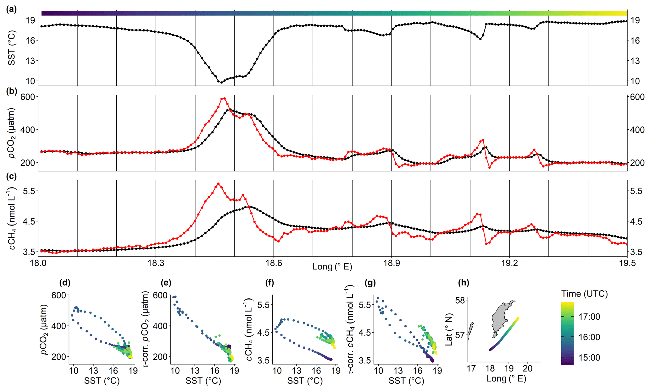
Figure A1 Demonstration of response time correction based on data from 24 August 2010 within the Go-SE box. The three upper plots display longitudinal patterns of (a) SST, (b) pCO₂, and (c) cCH₄. Black symbols are original values; red symbols are corrected using response times of ${\mathit{\tau }}_{{\mathrm{CO}}_{\mathrm{2}}}=\mathrm{226}$ s and ${\mathit{\tau }}_{{\mathrm{CH}}_{\mathrm{4}}}=\mathrm{676}$ s (Gülzow et al., 2011) and procedures according to Bittig et al. (2018). Panels (d–g) reveal relationships between (d) original and (e) τ-corrected pCO₂ and SST as well as (f) original and (g) τ-corrected cCH₄ and SST. Panel (h) displays the position of SOOP Finnmaid over time. Time is colour-coded to link all plots.

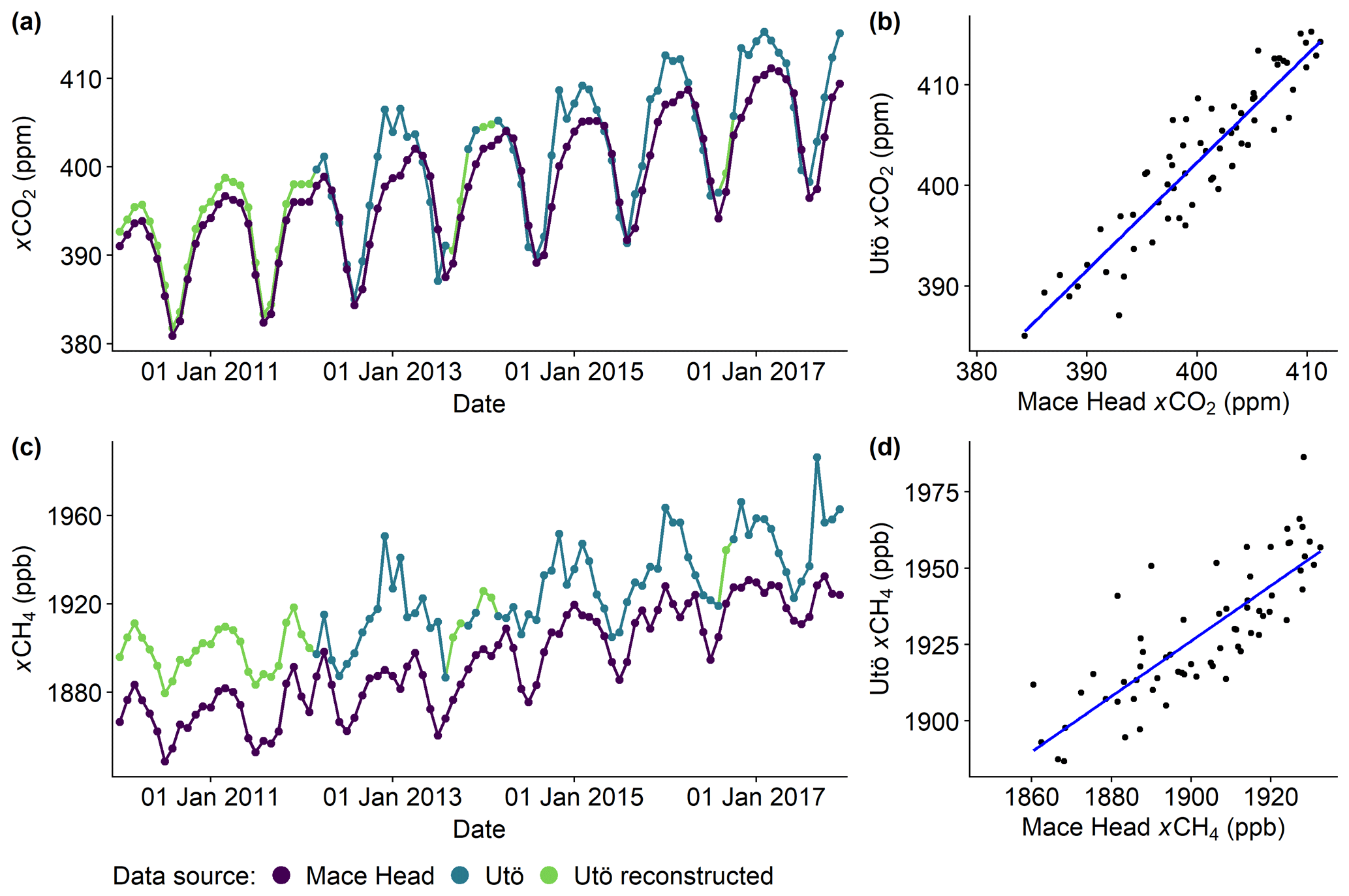
Figure A2 Monthly means of atmospheric (a) CO₂ and (c) CH₄ mole fractions from 2010 to 2017. We preferred data from Utö station (Finnish Meteorological Institute, Helsinki), which start in March 2012, due to their proximity to observations from SOOP Finnmaid. Concerning measurements on Utö, the method described in Kilkki et al. (2015) is applicable for the study period except that the Nafion dryer has not been in use since November 2013 (Juha Hatakka, personal communication, 2020). For the period before 2012 and to fill data gaps in September 2013 and 2016 in the Utö series, we used atmospheric data from Mace Head station (National University of Ireland, Galway) via the NOAA ESRL carbon cycle cooperative global air sampling network (Dlugokencky et al., 2019a, b), which is roughly at similar latitude. To correct differences between both stations, we normalised the data from Mace Head to those from Utö based on the shared period from 2012 to 2017 using linear regression (b, d). This very simple approach is sufficient to evaluate the magnitude of super- and undersaturation and compare it on interannual scales.

Figure A3 As Fig. 4 but based on model SST data from the entire box instead of along the sub-transect of SOOP Finnmaid. Please refer to Sect. 2.3 for a comparison to Fig. 4. Both approaches are further discussed in Sect. 3.1.

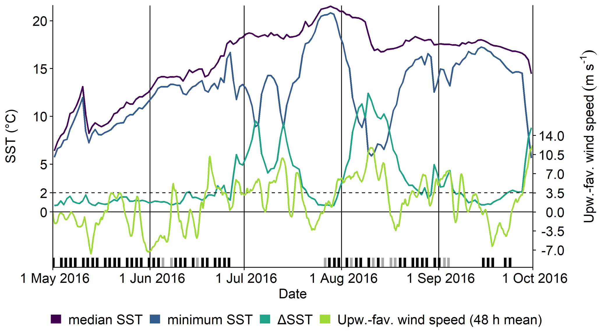
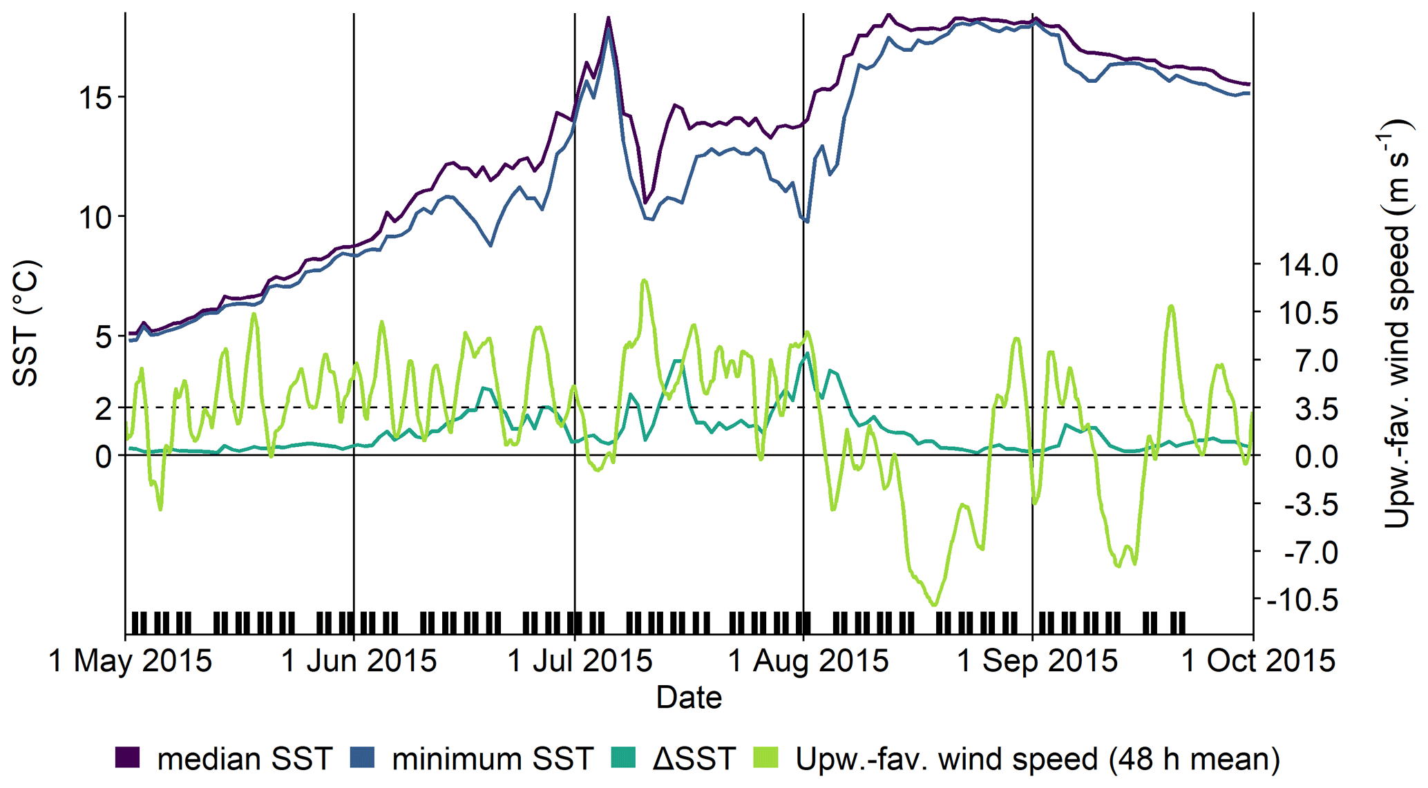
Figure A4 As Fig. 4 but within the Ö-S box in 2015 (here, both routes go through the box). Quasi-persistent upwelling-favourable wind conditions until the beginning of August effectively prohibited strong thermal stratification of the surface water. This results in lower possible SST gradients from upwelling and, therefore, a rather unreliable ΔSST criterion, which is only triggered during the most intense periods. Please refer to Sect. 3.4 for a detailed discussion of this event.

Appendix B: Results and discussion

B1 Calculation of theoretical relaxation and flux estimates

We calculated theoretical relaxation curves (Sect. 3.3) as follows: CO₂ system calculations were performed using the R package seacarb (Gattuso et al., 2019) with K₁ and K₂ from Millero (2010), K_w and K_f from Dickson and Riley (1979), and K_S from Dickson (1990); pCH₄ was calculated from cCH₄ (Wiesenburg and Guinasso, 1979). Since salinity changes by upwelling in the Baltic Sea are usually small (Lehmann and Myrberg, 2008), and no calcifying organisms are present (Schneider et al., 2014a), we assumed a constant salinity of 7 and a total alkalinity (A_T) of 1600 µmol kg⁻¹ (Müller et al., 2016). These along with the values for the initial (upwelled) water mass (SST=10 ^∘C, pCO₂=700 µatm, cCH₄=5 nmol L⁻¹) and the background water mass (SST=20 ^∘C, pCO₂=150 µatm, cCH₄=3.5 nmol L⁻¹) used for mixing are typical for late-summer upwelling in the central Go-SE box (Fig. 7d and l). However, as we mainly discuss the shapes of the curves, which are unaffected by variation in the input variables over a reasonable range, Fig. 8 is used to discuss processes in all regions.

Fluxes were calculated according to Wanninkhof (2014). We approximated the Schmidt number dependence on salinity via linear interpolation between the values for fresh water and seawater. In Sect. 3.3, we assume constant wind speeds of 10 m s⁻¹, SST=10 ^∘C, air temperature=20 ^∘C, relative humidity=0.8, and relative cloud coverage=0.8. In Sect. 3.5, we use the available wind data with 3 h resolution to calculate daily fluxes.

Figure B1 As Fig. 5, but further distinguished by year. ΔSST was calculated along the route of SOOP Finnmaid through the boxes (Sect. 2.3; second approach). Month abbreviations denote the period May–September.

Figure B2 As Fig. 5, but further distinguished by year and using a different ΔSST criterion, which was calculated based on the entire area of the boxes (Sect. 2.3; first approach). Month abbreviations denote the period May–September.

Figure B3 As Fig. 5, but using a different ΔSST criterion, which was calculated based on the entire area of the boxes (Sect. 2.3; first approach).

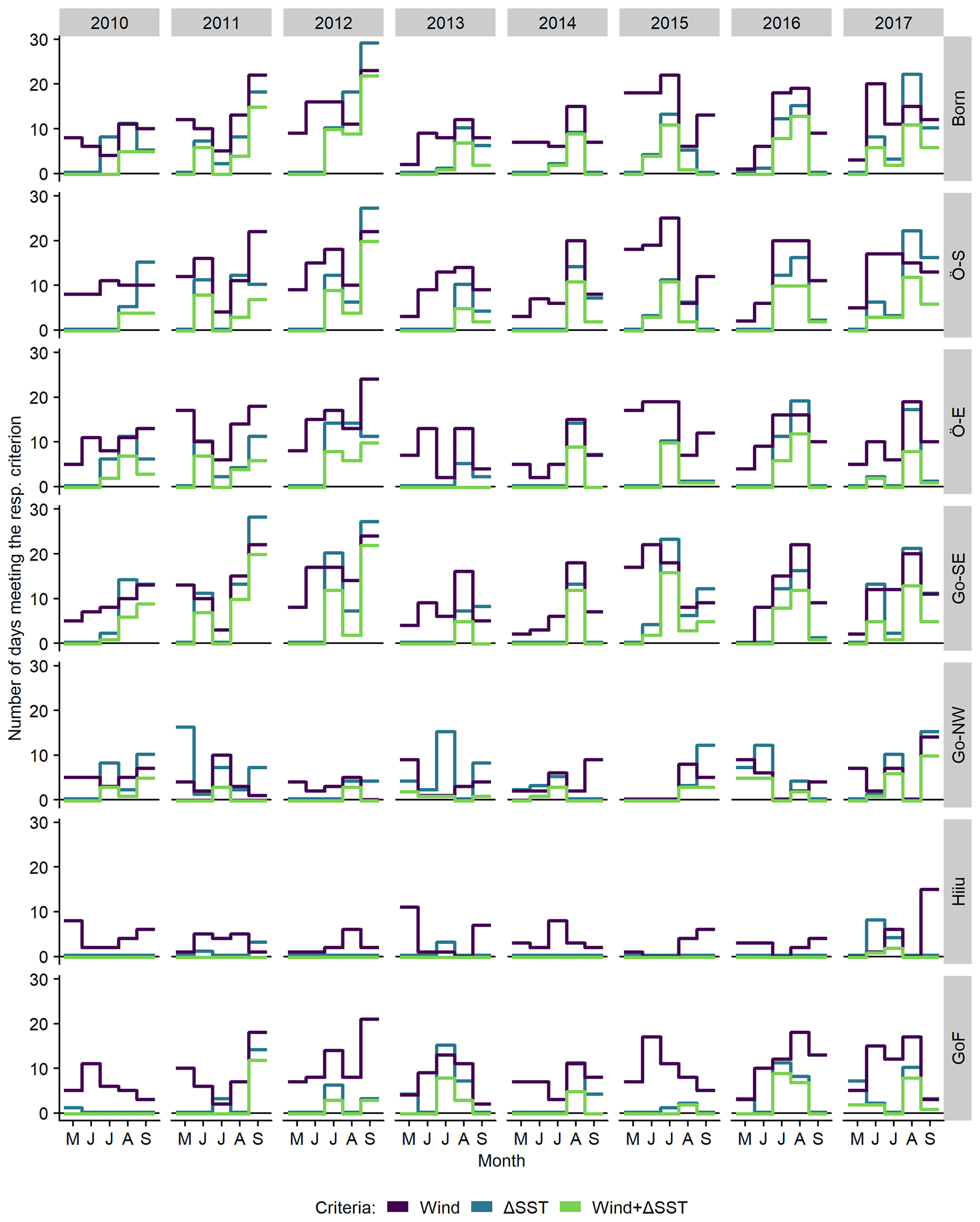
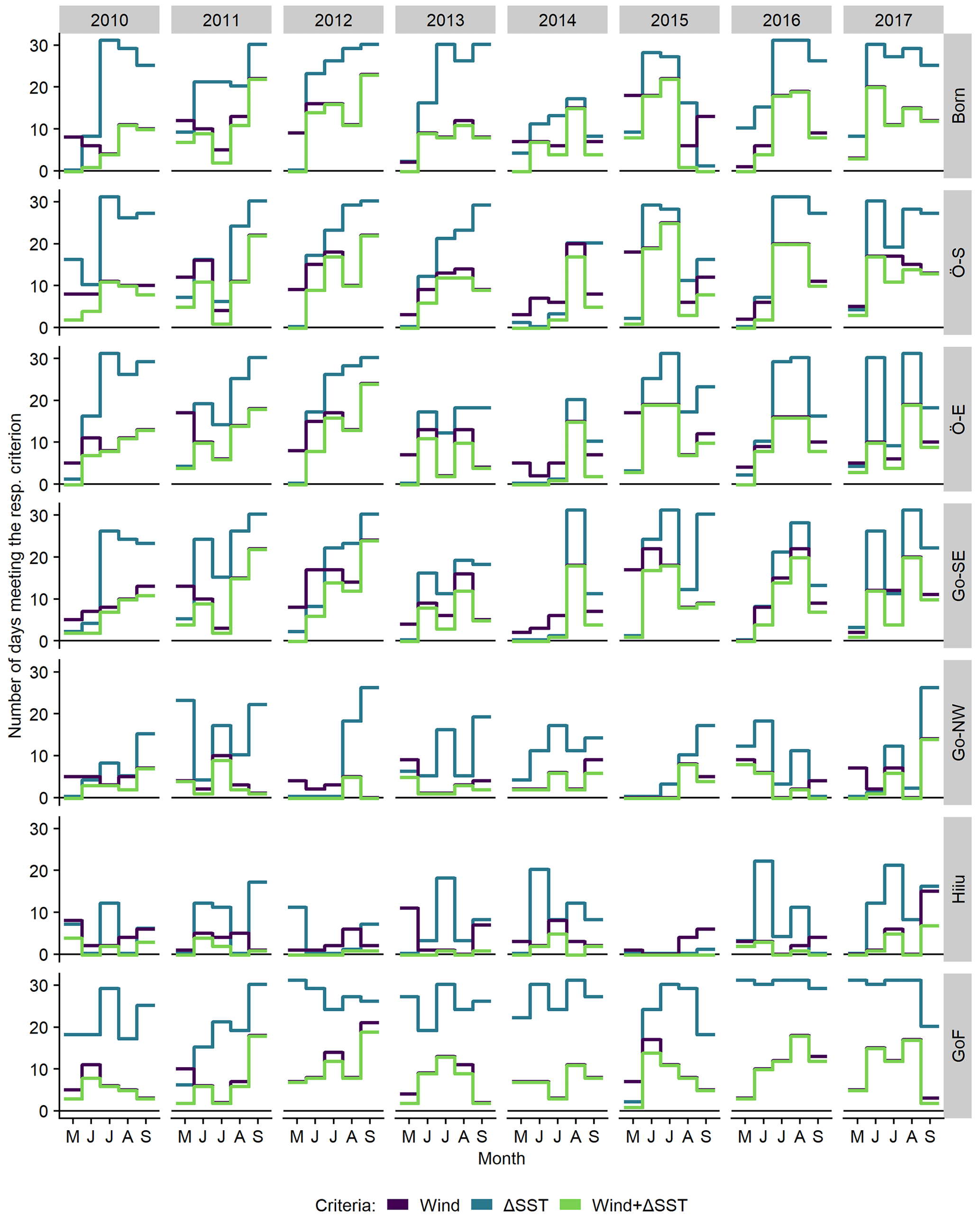
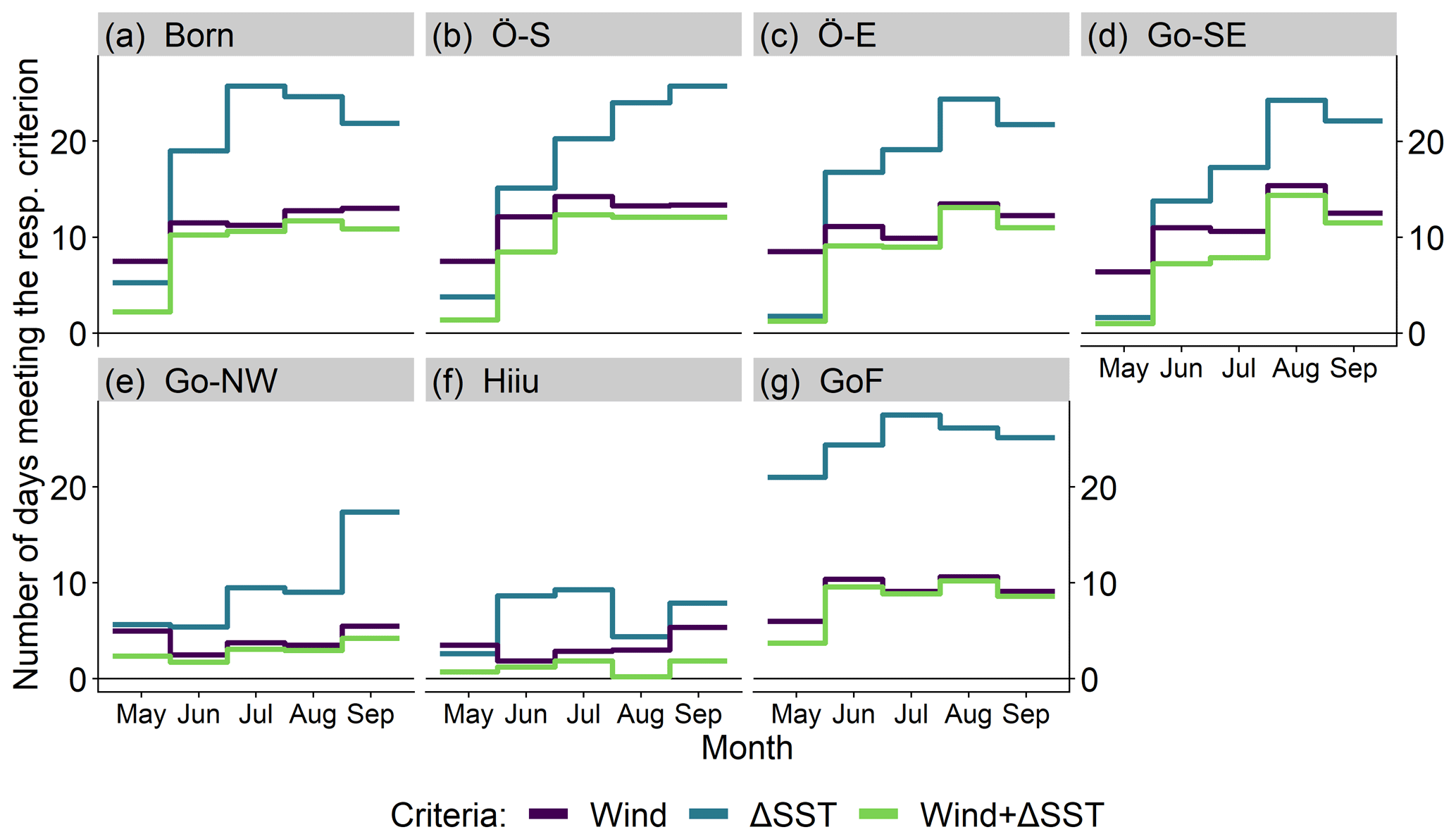
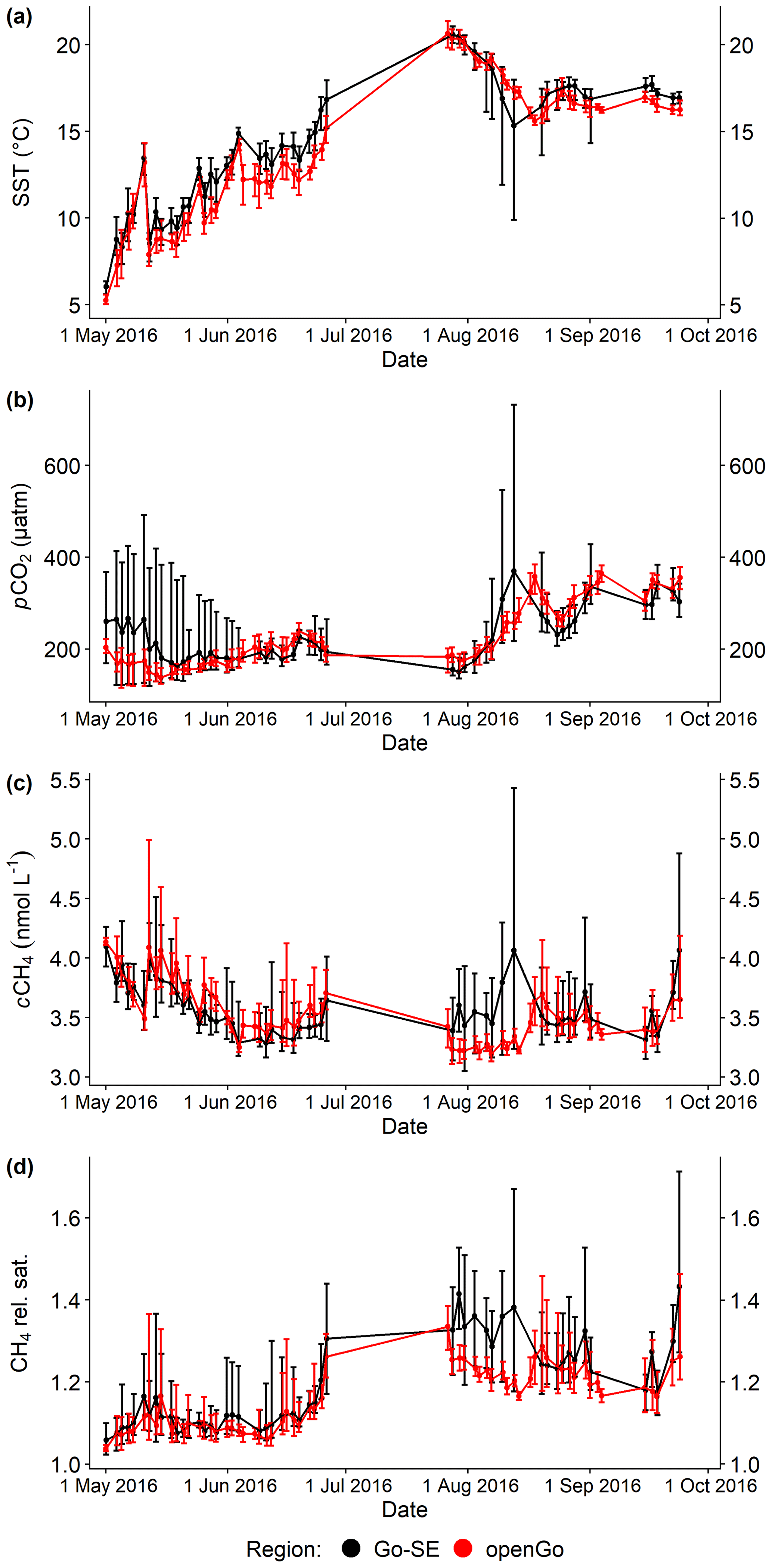
Figure B4 (a) Sea surface temperature, (b) CO₂ partial pressure, (c) CH₄ concentration, and (d) relative CH₄ saturation within the Go-SE (black) and openGo (red) boxes from 1 May to 23 September 2016. Points and lines represent mean values per sub-transect; error bars denote maximum and minimum, respectively. The effect of upwelling is very prominent in August 2016 (compare Fig. 4), when the Go-SE box features decreased SST and increased pCO₂, cCH₄, and relative CH₄ saturation values compared to the openGo box, which is not affected by upwelling.

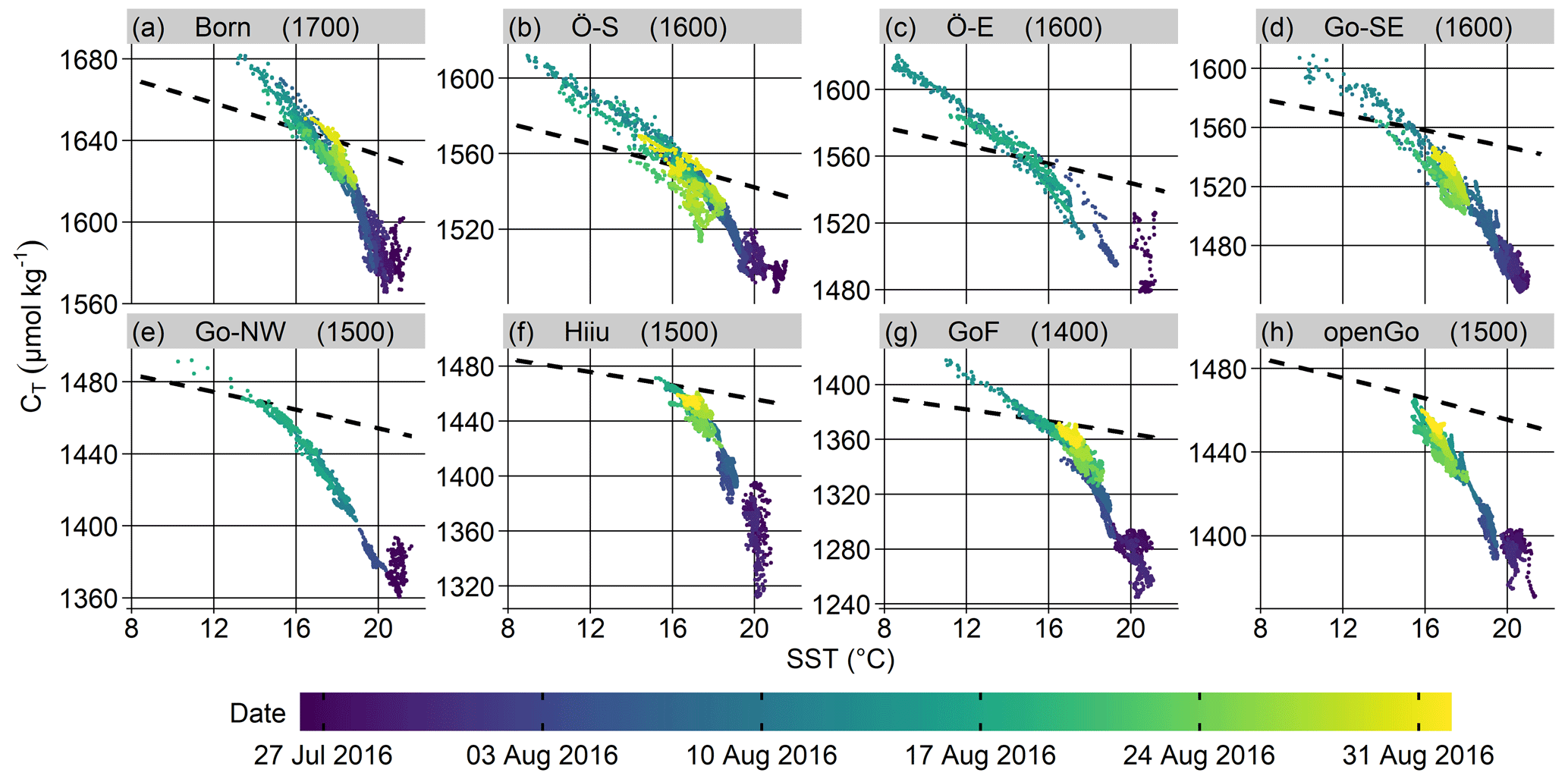
Figure B5 Surface C_T estimated from pCO₂ as measured by SOOP Finnmaid on 21 transects from 26 July to 30 August 2016, each plotted against SST within the seven upwelling regions and the open Gotland Sea box for comparison. We estimated A_T for each box (values in µmol kg⁻¹ in parentheses) based on Müller et al. (2016). The measurement date is colour-coded. Temporal coverage in the Go-SE box (15 transects) and the Ö-E and Go-NW boxes (6 transects) is reduced since SOOP Finnmaid uses two different routes around Gotland. Dashed black lines indicate atmospheric-equilibrium C_T (calculated using mean salinity per box in the given time period).

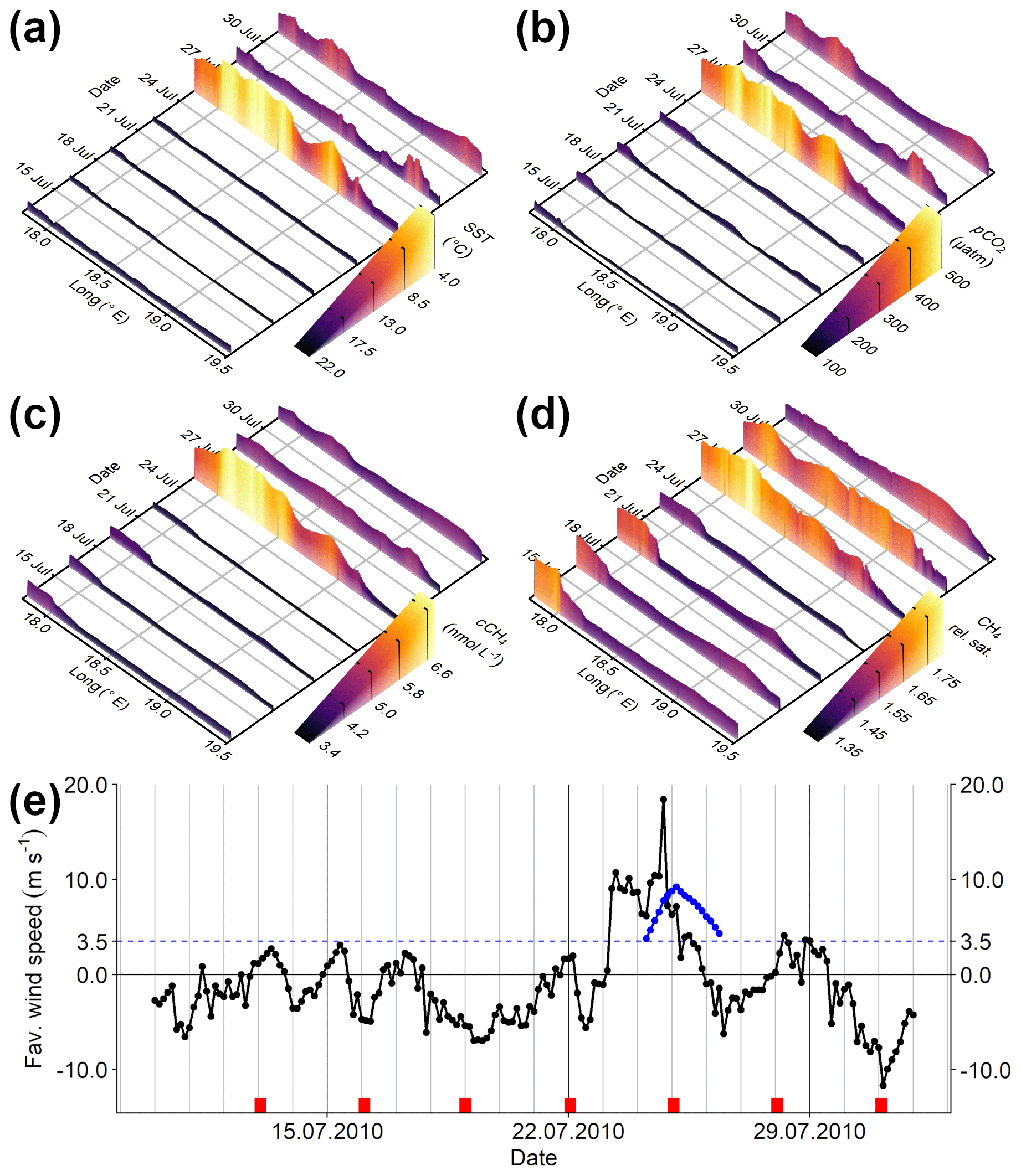
Figure B6 (a) Sea surface temperature, (b) CO₂ partial pressure, (c) CH₄ concentration, and (d) relative CH₄ saturation within the Go-NW box as measured by SOOP Finnmaid on seven transects from 12 to 31 July 2010. In (a–d), abscissa is position given as longitude, ordinate is time, and the respective variable is displayed by both colour and height of the curve. Please note the inverted SST scale in (a) to highlight the correlation between decreasing SST and increasing pCO₂ and cCH₄. (e) Upwelling-favourable wind component in the same period: black dots and lines are in 3 h intervals; blue dots represent the running 48 h mean if this mean is above 3.5 m s⁻¹. The dashed blue line indicates the chosen threshold of the wind criterion. Red dashes at the bottom mark transects of SOOP Finnmaid within the box (see a–d). This example shows distinct upwelling signals on 25 July, which vanish quickly after turning wind, hinting at downwelling as the relevant process for fast relaxation of upwelling signals. In fact, post-upwelling values of SST, pCO₂, and cCH₄ differ only slightly from pre-upwelling values.