Estimating immediate post-fire carbon fluxes using the eddy-covariance technique

Wildfires typically affect multiple forest ecosystem services, with carbon sequestration being affected both directly, through the combustion of vegetation, litter and soil organic matter, and indirectly, through perturbation of the energy and matter balances. Post-fire carbon fluxes continue to be poorly studied at the ecosystem scale, especially during the initial window of disturbance when changes in environmental conditions can be very pronounced due to the deposition and subsequent mobilization of a wildfire ash layer and the recovery of the vegetation. Therefore, an eddy-covariance system was installed in a burnt area as soon as possible after a wildfire that had occurred on 13 August 2017 and has been operating from the 43rd post-fire day onwards. The study site was specifically selected in a Mediterranean woodland area dominated by maritime pine stands with a low stature that had burned at high severity.

The carbon fluxes recorded during the first post-fire hydrological year tended to be very low so that a specific procedure for the analysis and, in particular, gap filling of the eddy-covariance data had to be developed. Still, the carbon fluxes varied noticeably during the first post-fire year, broadly revealing five consecutive periods. During the rainless period after the wildfire, fluxes were reduced but, somewhat surprisingly, indicated a net assimilation. With the onset of the autumn rainfall, fluxes increased and corresponded to a net emission, while they became insignificant with the start of the winter. From the midwinter onwards, net fluxes became negative, indicating a weak carbon update during spring followed by a strong uptake during summer. Over the first post-fire year as a whole, the cumulative net ecosystem exchange was −347 g C m⁻², revealing a relatively fast recovery of the carbon sink function of the ecosystem. This recovery was mainly due to understory species, both resprouter and seeder species, since pine recruitment was reduced.

Specific periods during the first post-fire year were analyzed in detail to improve process understanding. Perhaps most surprisingly, dew formation and, more specifically, its subsequent evaporation were found to play a role in carbon emissions during the rainless period immediately after fire, involving a mechanism distinct from degassing the ash–soil pores by infiltrating water. The use of a special wavelet technique was fundamental for this inference.

1 Introduction

The increasing frequency and intensity of extreme climate events (IPCC, 2018) are contributing to an increase in frequency and severity of wildfires (Flannigan et al., 2013; Keeley and Syphard, 2016). Such unprecedented wildfire regimes have been causing widespread concerns about their socioeconomic and environmental impacts, including damages to ecosystems and the services they provide (Moritz et al., 2014). An important ecosystem service that is impacted by wildfires is carbon sequestration by forests (Campbell et al., 2007; Restaino and Peterson, 2013). Thereby, wildfires can interfere with forest policy and management goals for climate change mitigation (Restaino and Peterson, 2013; Ruiz-Peinado et al., 2017).

Wildfires impact forest carbon pools not only directly through combustion of vegetation and litter biomass and soil organic matter but also indirectly through disturbance of energy, water and carbon fluxes (Sommers et al., 2014; Stevens-Rumann et al., 2017). These indirect effects are particularly difficult to assess, as they depend on a number of factors related to fire severity, forest type, post-fire land management and post-fire environmental conditions (De la Rosa et al., 2012; Santana et al., 2016; Serrano-Ortiz et al., 2011). Furthermore, these effects can be long lasting, as illustrated by Dore et al. (2008), finding that a Pinus ponderosa forest was a carbon source 10 years after a stand-replacing wildfire (Table S1 in the Supplement).

In their review of 2013, Restaino and Peterson (2013) argued that relatively few studies had assessed post-fire carbon dynamics through the measurement of carbon fluxes as opposed to changes in carbon pools and that relatively few of these flux studies had used the eddy-covariance (EC) technique. Marañón-Jiménez et al. (2011) likewise affirmed that post-fire studies of soil carbon effluxes were relatively abundant. To date, EC studies following wildfires have continued to be scarce (Amiro, 2001; Dadi et al., 2015; Dore et al., 2008; Mkhabela et al. 2009; Serrano-Ortiz et al., 2010; Sun et al., 2016). Furthermore, only the study of Sun et al. (2016) concerned the immediate post-fire period, with EC measurements starting from the fourth month after fire. To address this knowledge gap, this study aimed to investigate carbon fluxes of a maritime pine forest during the first hydrological year after wildfire using a flux tower, in particular after a high-severity wildfire, as indicated by complete consumption of the crowns of the pine trees (following Maia et al., 2012). Because of the lack of comparable studies and because marked changes were expected in both abiotic and biotic conditions due to mobilization of wildfire ash and/or vegetation recovery, a specific objective of the present study was to get a better understanding of the different processes governing these immediate-post-fire carbon fluxes. The short study period, its dynamic conditions and the generally very small fluxes implied the need for specific, non-standard data quality tests and gap-filling procedures, especially to avoid the excessive replacement of measured fluxes by fluxes estimated with – poorly parameterized – gap-filling equations.

2 Materials and methods

2.1 Study area

Figure 1 Slope angle map derived from aerial photography of the burnt area surrounding the flux tower. The imagery was acquired on 18 July 2018, using the standard RGB camera mounted on a DJI Phantom 3 drone.

The study area (39^∘37^′ N, 08^∘06^′ W) was located in Vila de Rei, Portugal, in a Mediterranean climate zone at the transition of Köppen–Geiger classes Csa and Csb, with dry summers and an average temperature of 22 ^∘C in the warmest month (Kottek et al., 2006). The study area was selected on 2 September 2017 for three main reasons: (i) for having been severely affected by a recent wildfire, (ii) for being dominated by maritime pine (Pinus pinaster Ait.) stands of comparatively low stature (≤ 10 m) and (iii) for consisting of relatively flat terrain within the presumed footprint area. Tree species and height were preselected based on the available, slim tower of 12 m high. The study area was a plateau of sedimentary sandstone deposits, at an elevation of 240–250 $\mathrm{m}\mathrm{a}.\mathrm{s}.\mathrm{l}.$ (Fig. S1a in the Supplement), with slopes of up to 5^∘ over an extension of approximately 10 ha (Fig. 1).

The wildfire affecting the study area occurred on 13 August 2017 and burned some 12.5 km² of woodland in total (ICNF, 2017). According to the European Forest Fire Information System (EFFIS, 2017), the fire severity in the study area varied between moderate and high. Fire severity was also assessed in the field, on 9 September 2017, along a 500 m transect that was laid out to the west of the slim tower, in the central part of the presumed footprint area (Fig. S1b). More specifically, severity was determined at five points along the transect and, at each transect point, for three plots centered on the nearest pine tree and the nearest shrub and the inter-patch in between. At all five transect points, crown consumption of the pine trees exceeded 75 %; undergrowth vegetation and litter were fully consumed; and wildfire ash was predominantly black. The ash layer varied in depth between 0.4 and 1.0 cm and in cover between 55 % and 100 %. Soil burn severity at the 15 plots was classified according to Vega et al. (2013) and ranged from moderate to high (class 3) at 8 plots to high (class 4) at 7 plots.

Figure 2 Ortho-photomap of the study area showing the eucalypt stands as well as the four individual eucalypt specimens close to the slim tower (EC tower; circle with cross). The rest of the area consists of maritime pine stands. The imagery was acquired on 18 July 2018, using a standard RGB camera mounted on a DJI Phantom 3 drone.

A map of tree species in the study area was made through photo-interpretation of an ortho-photomap produced from aerial photographs that had been acquired with an RGB camera mounted on a drone (DJI Phantom 3, SZ DJI Technology Co., Ltd., Shenzhen, PR China) on 18 July 2018. Maritime pine stands covered 90 % of the presumed footprint area, while eucalypt (Eucalyptus globulus) stands occupied the remaining 10 % (Fig. 2). Also, during July 2018, the pine stands in the footprint area were characterized, using five plots of 5 m × 5 m centered on the pine trees of the abovementioned fire severity assessment. Median height and diameter at breast height of the burnt pine trees in each of the five plots selected for the fire severity assessment ranged from 4.6 to 6.7 m and from 2.5 to 4.3 cm, respectively. The maximum height of the trees was 7.8 m in median, ranging from 5.4 to 12.1 m in the individual plots. The densities of living pines varied from 0.24 to 1.72  trees m⁻² before fire to 0.12 to 1.04 seedlings m⁻² after fire. This decrease in density by the fire could be explained by the young age of the stands (in median, 12–15 years), in combination with fire damage to the (aerial) seed bank, in line with the extensive combustion of the pine crowns (Maia et al., 2012). The density of resprouting shrubs ranged from 0.0 to 0.16  shrubs m⁻² (details on vegetation composition are given in Table S2 in the Supplement).

2.2 Experimental setup

Figure 3 Wind rose of the study area over the first post-fire hydrological year (1 October 2017–30 September 2018), based on the sonic anemometer measurements at 11.6 m height.

After obtaining authorization from the landowners, the study area was instrumented with an eddy-covariance system mounted on a slim tower and powered by four solar panels. The system was installed on 22 September 2017 and started operating 4 d later, i.e., 43 d after the wildfire. The exact location of the tower and the height and orientation of the gas analyzer and 3-D anemometer were determined on the basis of the available regional climate information, indicating a prevalence of northwesterly winds. This was confirmed by the measurements during the first post-fire year, as shown in Fig. 3.

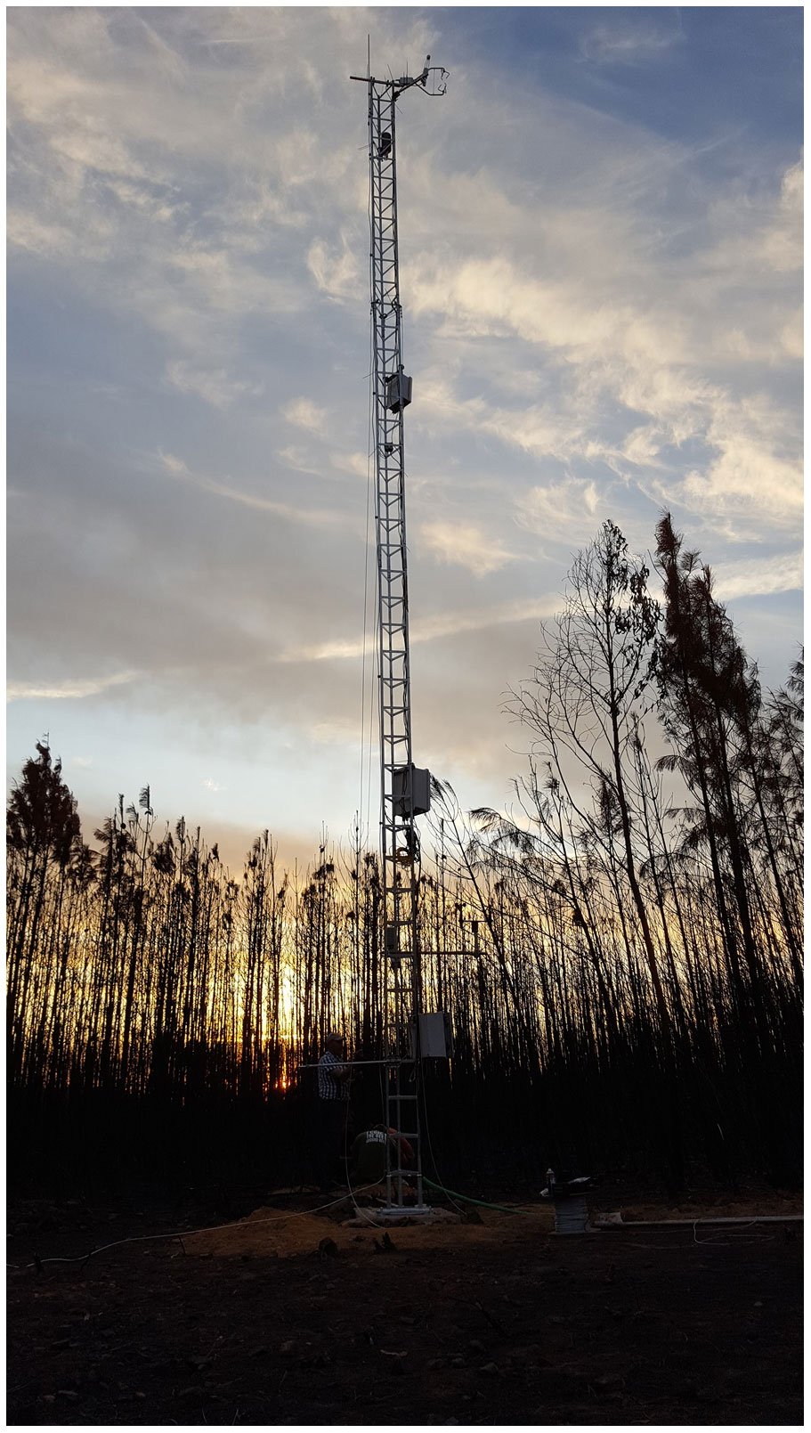
Figure 4 The 12 m slim tower with the eddy-covariance system immediately after its installation (photograph: J. Jacob Keizer, 22 September 2017).

Table 1 Meteorological sensors mounted on the slim tower and in its immediate surroundings.

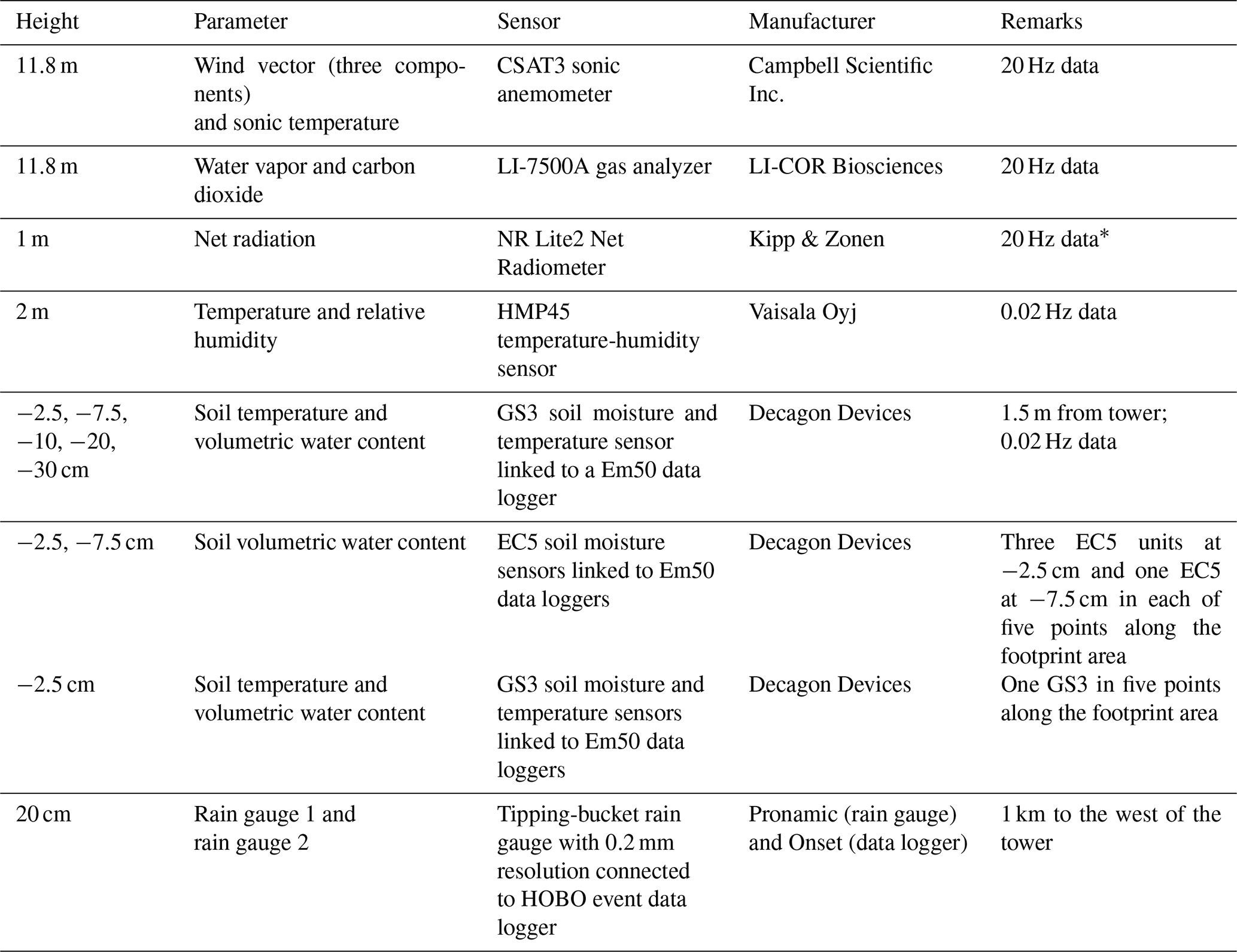
^∗ No 0.02 Hz channel was free for logging the net radiation.

A picture of the tower immediately after installation is shown in Fig. 4, while the installed devices are listed in Table 1. The – standing – pine trunks in the immediate surroundings of the tower were approximately 8 m high (also in line with the abovementioned median of 7.8 m for the maximum tree height in the presumed footprint area), and this was used as “canopy” height in all calculations, together with a zero-plane displacement of 3.8 m. The data for the calculation of the turbulent fluxes were sampled and stored at 20 Hz using a CR6 data logger from Campbell Scientific Ltd., while the fluxes were calculated over 30 min intervals. All other data were sampled at 0.02 Hz, stored at 15 min intervals and then averaged over the 30 min intervals, except for rainfall. Rainfall was recorded using two automatic rainfall gauges with a 0.2 mm resolution and then summed over the 30 min intervals. In addition to the soil moisture/temperature station immediately next to the tower, a soil moisture and temperature station was installed at each of the five transect points (Fig. S1b). Each station comprised four EC5 soil moisture sensors and one GS3 soil moisture and temperature sensor. Three of a station's EC5 sensors were inserted horizontally into the soil at 2.5 cm depth; one was immediately next to a burnt pine tree; one was immediately next to a resprouter shrub (Pterospartum tridentatum); and one was at a bare inter-patch. The fourth EC5 sensor and the GS3 sensor were also installed at the inter-patch, at a depth of 2.5 and 7.5 cm, respectively. In this study, only the data from the EC5 sensors installed at −2.5 cm depth at the five inter-patches were used.

This study focuses on the first hydrological year after the wildfire, from 1 October 2017 to 30 September 2018. The preceding data from 26 to 30 September 2017 were only used for one of the specific cases that were analyzed in more detail to improve process understanding (Sect. 3.1.1).

2.3 Eddy-covariance data

2.3.1 Data calculation

The eddy-covariance (EC) method is well-established for calculating energy and matter fluxes between the atmosphere and the underlying surface (Aubinet et al., 2012). Therefore, the applied procedures are only briefly described. The 30 min EC values were calculated automatically by the Campbell EasyFlux software in the CR6 data logger but just for checking the operational status of the system. The calculations presented here were done using the software package TK3 (Mauder and Foken, 2015), which was found to compare well with other packages (Fratini and Mauder, 2014; Mauder et al., 2013). All corrections to the EC values were done following the recommendations by Foken et al. (2012) and involved spike detection, time delay correction, double rotation, and SND (Schotanus, Nieuwstadt and DeBruin) and WPL (Webb, Pearman and Leuning) correction (Schotanus et al., 1983; Webb et al., 1980). The quality of the flux data was checked following the method by Foken and Wichura (1996) and using the latest published version of the flagging system (Foken et al., 2012). This procedure was also used in gap filling (Ruppert et al., 2006). The CO₂ storage flux is estimated by TK3 from one-point CO₂ measurements, as suggested by Hollinger et al. (1994). Finally, all 30 min values were checked by means of a MAD (median absolute deviation) analysis (Papale et al., 2006).

The footprint area was determined with the model of Kormann and Meixner (2001). More than 25 % of the EC measurements coincided with more than 80 % of the maritime pine stands, whereas 60 % of the measurements coincided with more than 60 % of the maritime pine stands (Fig. 5). Both percentages are high in comparison with the literature (Göckede et al., 2008).

Basic EC data analysis and, in particular, gap filling were done using the data that met quality classes 1–6 (Foken et al., 2012) and had footprint areas that consisted of more than 80 % of the maritime pine stands, as shown in the flow diagram of Fig. S2 in the Supplement. The same criteria were used for selecting the specific cases presented in Sect. 3. For the cumulative fluxes over the first post-fire year, all EC data with quality classes 1–8 were combined with gap-filled data, following the procedure shown in Fig. S3 in the Supplement. The contribution of the eucalypt patches and trees in the footprint area to observed carbon fluxes was investigated in Sect. 3.1.3.

2.3.2 MAD test

In order to eliminate some outliers (spikes) from the data selected for parameterization in the gap-filling procedure, the MAD test (MAD – median absolute deviation) was applied. The MAD test according to Hoaglin et al. (2000) was first applied to CO₂ flux data by Papale et al. (2006) and first used for despiking raw EC data by Mauder et al. (2013). The MAD test identifies as outlier all values that are outside the following range:

$$\begin{array}{}\text{(1)}& \text{median}\left(x\right)-{\displaystyle \frac{q\text{MAD}}{\mathrm{0.6745}}}<x_i<\text{median}\left(x\right)+{\displaystyle \frac{q\text{MAD}}{\mathrm{0.6745}}},\end{array}$$

where the factor of 0.6745 stems from the Gaussian distribution and q is a threshold value that must be determined depending on the specific data set.

2.3.3 Spike test

The spike test was used in the final stage of data processing (Fig. S3). While the MAD test is used when the measured values to be examined scatter only slightly around a mean value, the spike test is used for more scattering data. This test determines the SD (standard deviation) of the entire data set and excludes all values that deviate by a multiple of the SD. For the spike test, a factor of 3.5 was used as the threshold, following Højstrup (1993). The spike test must be carried out multiple times until the SD hardly changes, which happened after 2–4 times in this study.

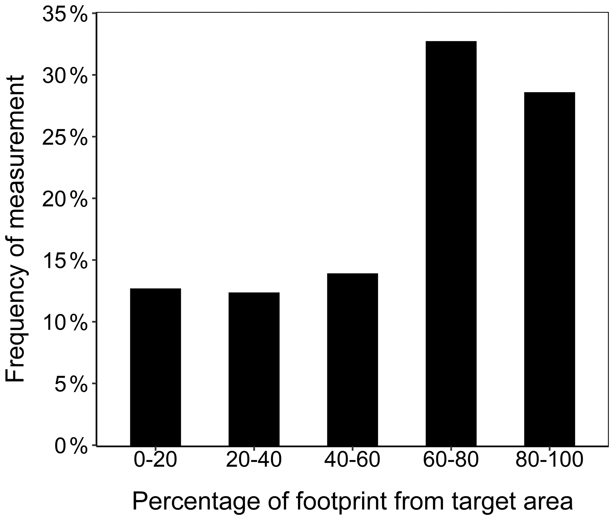
Figure 5 Distribution of the eddy-covariance measurements during the first post-fire hydrological year over five classes of the footprint area based on the degree of correspondence to the maritime pine stands.

2.3.4 Turbulent fluxes with high temporal resolution

The wavelet-based flux computation method was used to analyze a short-term flux event with non-steady-state fluxes during the rainless period immediately after the wildfire. This method offers the possibility of determining fluxes with a temporal resolution as high as 1 min (Schaller et al., 2017). The wavelet method agrees well with the EC method for steady-state conditions and was successfully applied to analyze short events of high methane fluxes in the recent studies of Göckede et al. (2019) and Schaller et al. (2019).

The wavelet method in this study applied the Mexican hat wavelet, as it provides an excellent resolution of the fluxes in the time domain and identifies the exact moment in time when single events occur (Collineau and Brunet, 1993). The wavelet method was applied using spike-free and coordinate-rotated 1 min data. Furthermore, the cone of influence (Torrence and Compo, 1998) was estimated to guarantee that the results were not affected by edge effects.

2.3.5 Influence of mechanical turbulence

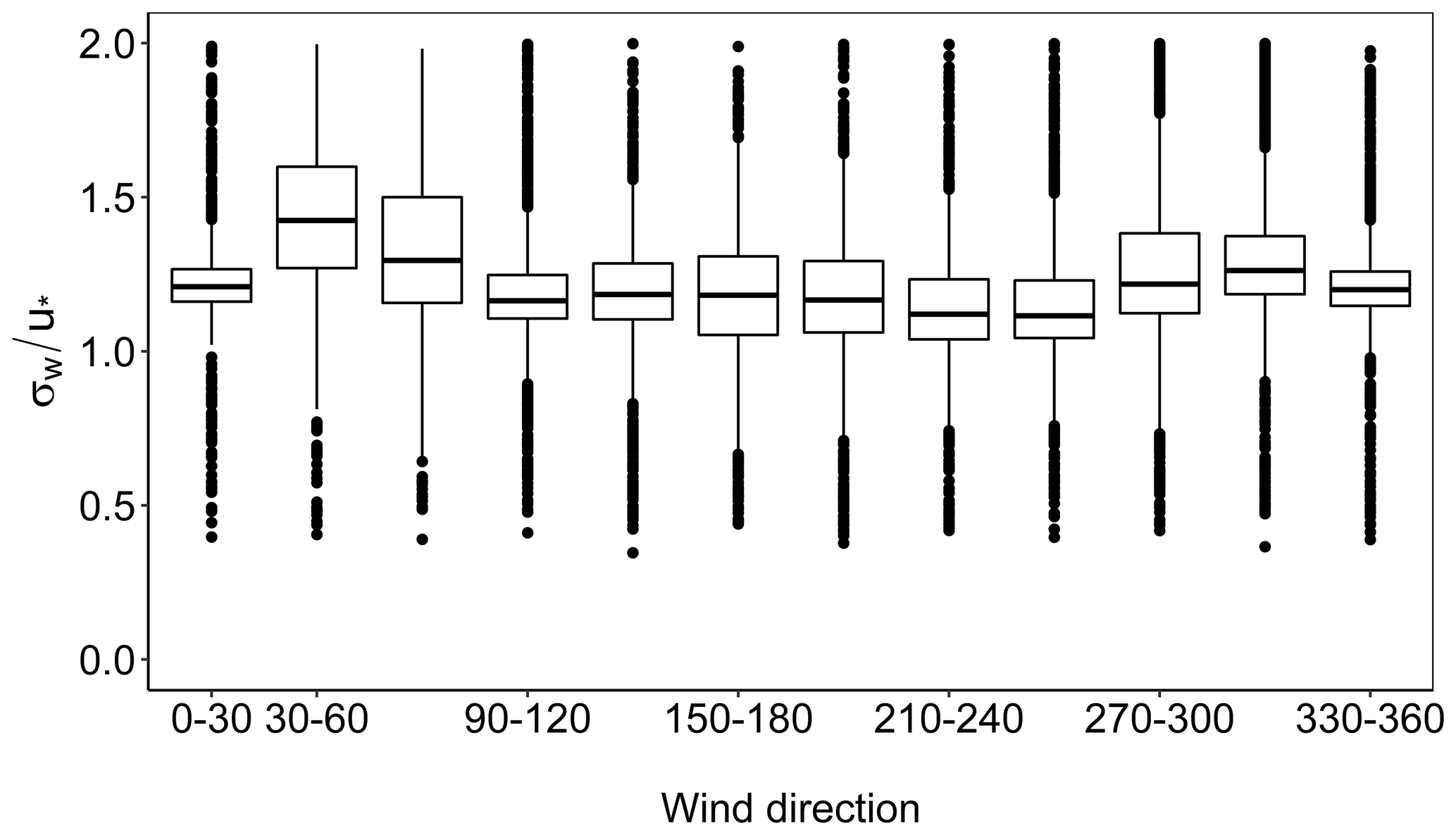
Figure 6 Box plots of the normalized SD of the vertical wind velocity (${\mathit{\sigma }}_{\mathbf{w}}/u_{\ast }$) for the individual wind direction sectors.

The fact that the bulk of the burnt tree trunks continued upright during the study period raised concerns about their possible impact on turbulence conditions. Therefore, mechanical turbulence was tested according to Foken and Leclerc (2004). The test parameter is the SD of the vertical wind velocity normalized by the friction velocity ${\mathit{\sigma }}_{\mathrm{w}}/u_{\ast }$ and was also used here in the quality flagging of the turbulent data (Sect. 2.3.1). The test was carried out with 12 011 30 min records (68 % of the data without selection of the footprint) that were selected for conditions of neutral stratification (−0.2 $<z/L<\mathrm{0.1}$) and data quality classes 1–8 (i.e., without footprint selection). The average and SD of ${\mathit{\sigma }}_{\mathrm{w}}/u_{\ast }$ were 1.19 and 0.16, which agreed with available parameterizations (Foken, 2017; Panofsky et al., 1977). The data also confirmed the dependency of the test parameter on stratification (not shown here). The distribution of the test parameter according to wind direction (Fig. 6) revealed higher median values for the 30–60^∘ and 60–90^∘ sectors. This could be explained as the typical effect of wind flowing through the tower and coming from the back side of the sonic anemometer, in line with Li et al. (2013). Furthermore, the large patch of eucalypt trees in the 30–60^∘ sector (Fig. 2) could have caused additional turbulence, especially as they resprouted vigorously soon after the fire. The method applied for data treatment also flagged data from these sectors. The parameter values for the other wind sectors suggested a tendency for lower median values for the sectors between 210 and 270^∘ and higher median values for the sectors between 270 and 30^∘, possibly caused by downhill and uphill flows, respectively (Fig. 1). In overall terms, the values were within the typical range and did not suggest that the standing trunks of either pines or eucalypts had a relevant impact on data quality.

2.3.6 Energy balance closure

The energy balance, defined as the sum of the turbulent sensible and latent heat fluxes, the net radiation and the ground heat flux, is not fully closed for many turbulent flux sites for multiple reasons that are in most cases not related to measuring errors (Foken, 2008; Mauder et al., 2020). The energy balance closure check serves to verify the general data quality of the flux measurements and should be in the usual closure gap range of < 30 % (Foken et al., 2012). In the case of the present study site, 24 June 2018 (with solar noon at 12:38 UTC) was a typical example of a day with a mostly clear sky, even if some influence of high clouds was suggested by the comparison of net radiation and sensible heat flux (Fig. S4 in the Supplement). On average, there were nearly no residuals; however, residuals that reached values of up to 100 W m⁻² occurred in the afternoon, and those that reached even up to about 200 W m⁻² occurred in the morning. The most likely reason for these discrepancies is that errors occurred in the calculation of the ground heat flux (Sect. 2.5). The calculation of ground heat flux from soil temperature and volumetric moisture content may be less appropriate for a post-fire condition. More specifically, the present experimental setup ignored the presence of a – black – wildfire ash layer and may not have fully captured the soil temperature gradient. This gradient was possibly steep in the first few mm, especially when the soils were dry and still covered by wildfire ash and not yet by vegetation, due to the increased direct insolation combined with a low soil heat capacity and conductance. While the possibility that the net radiation measurements suffered from a slight inclination of the radiometer (in a southwestern direction) cannot be altogether excluded, net radiation did appear to be underestimated. Net radiometers, as the one used in this study (Table 1), which do not measure the four up- and downwelling long- and shortwave radiation components separately, are well-known to underestimate net radiation (Kohsiek et al., 2007). In the case of the model preceding the one used in this study (i.e., the NR Lite1 Net Radiometer), Brotzge and Duchon (2000) reported underestimations of up to 100 W m⁻² at noon, with a strong sensitivity to the wind speed. The prevalence of negative residual fluxes during the morning was in line with an underestimation of the net radiation due to strong upwelling longwave radiation as a result of high surface temperatures, producing a bias that should be smaller during the afternoon. Because of this possible bias in the closure of the energy balance, a MAD test was applied to the ratio of the turbulent fluxes and the available energy (i.e., net radiation minus ground heat flux), with a factor q=0.5 having been selected as optimal (Sect. 2.3.2). As shown in Fig. S5 in the Supplement, the gap in energy balance closure amounted to about 10 %, which is within the range of typical values. Therefore, energy balance closure was considered not to pose a significant problem in the calculation of the fluxes.

Turbulent fluxes may also need to be corrected depending on the ratio of sensible and latent heat fluxes, i.e., the Bowen ratio. In the case of a Bowen ratio larger than 1, the sensible heat flux is assumed to be underestimated; in the case of a Bowen ratio below 1, both sensible and latent heat fluxes are assumed to be affected (Charuchittipan et al., 2014; Mauder et al., 2020). As shown in Fig. S6 in the Supplement, almost all EC measurements under the driest soil conditions (VWC classes 1 and 2; volumetric water content) had a Bowen ratio larger than 1, whereas the same was true for roughly three-quarters of the measurements under intermediate and wet soil conditions (VWC classes 3 and 4). Therefore, the latent heat flux was not substantially affected, and, hence, the CO₂ fluxes did not need further correction.

2.4 Gap filling of respiration and assimilation

2.4.1 Basic equations

The gap-filling procedure used for substituting missing data as well as data of low quality was based on the Lloyd–Taylor and Michaelis–Menten functions, as it is a well-established procedure (Falge et al., 2001; Gu et al., 2005; Hui et al., 2004; Lasslop et al., 2010; Moffat et al., 2007; Reichstein et al., 2005).

The Lloyd–Taylor function was used to calculate respiration, Q_R:

$$\begin{array}{}\text{(2)}& Q_{\mathrm{R}}=Q_{\mathrm{R},\mathrm{10}}\exp \left[E_{\mathrm{0}}\left({\displaystyle \frac{\mathrm{1}}{\mathrm{283.15}-T_{\mathrm{0}}}}-{\displaystyle \frac{\mathrm{1}}{T-T_{\mathrm{0}}}}\right)\right],\end{array}$$

where T is the temperature, Q_R,10 is the respiration at 10 ^∘C, and T₀ is 227.13 K and describes the temperature dependence of respiration (Falge et al., 2001; Lloyd and Taylor, 1994). The parametrization of Q_R,10 and E₀ was done using the nighttime CO₂ flux data, when assimilation is zero. The nighttime period is typically determined based on a threshold of global radiation, but since only net radiation was measured in this study, nighttime was defined here as the time window from 22:00 to 04:00 UTC (UTC nearly being the local time at the study site). The parameter values were then determined using the median fluxes of 5 K temperature intervals.

The parametrization of the carbon uptake at daytime, Q_c, day, was done with the Michaelis–Menten function (Falge et al., 2001; Michaelis and Menten, 1913), which must be determined for separate classes of temperature and global radiation:

$$\begin{array}{}\text{(3)}& Q_{\mathrm{c},\text{day}}={\displaystyle \frac{a{R}_{\mathrm{n}}{Q}_{\mathrm{c},\text{sat}}}{a{R}_{\mathrm{n}}+Q_{\mathrm{c},\text{sat}}}}+Q_{\mathrm{R},\text{day}},\end{array}$$

where Q_c, sat is the carbon flux at light saturation, R_n is the net radiation corrected with the longwave net radiation (as global radiation was not measured; see below), Q_R, day is the respiration at daytime and a is the linear slope of the assimilation function beginning at a global radiation of 0 W m⁻² (Falge et al., 2001; Michaelis and Menten, 1913). The constants a and Q_c, sat were determined by multiple regression for separate classes of temperature and corrected net radiation.

Since global radiation was not measured in this study, assimilation was gap-filled using the net radiation corrected with the longwave net radiation for an assumed cloud height of 2–4 km and assuming a low albedo of the surface, following

$$\begin{array}{}\text{(4)}& R_{\mathrm{n}-\text{corr}}=R_{\mathrm{n}}+{\mathit{\sigma }}_{\text{SB}}\left[T^{\mathrm{4}}-(T-\mathrm{20}{)}^{\mathrm{4}}\right],\end{array}$$

where σ_SB is the Stefan–Boltzmann constant and T is the temperature at 11.8 m height. This procedure is based on the data quality check for longwave radiation (Gilgen et al., 1994).

2.4.2 Respiration

Standard approaches for gap filling were assumed to be less adequate for the present study for two reasons: (i) the marked recovery of the above-ground vegetation in the course of the observation period, in particular from early spring 2018 onwards, and (ii) the important role of soil moisture content in soil respiration fluxes, as is typical for Mediterranean and dry ecosystems (Richardson et al., 2006; Sun et al., 2016). The latter was confirmed by a preliminary analysis of the nighttime net ecosystem exchange (NEE) fluxes for the different soil VWC classes (not shown but evident in Fig. 7) so that the gap filling was done separately for very dry to dry soil conditions (VWC classes 1 and 2) and for intermediate to wet (VWC classes 3 and 4) conditions. Respiration fluxes were determined using only the measurements from 22:00 to 04:00 UTC to reduce the influence of the additive WPL correction (Webb et al., 1980), with more than 80 % of the footprint area from the maritime pine stands and with quality flags 1–6. The selected measurements were subsequently subjected to a MAD test, following Papale et al. (2006) and using q=0.5 (Eq. 1). The Q₁₀ and E₀ parameters for the two VWC categories were estimated using the median fluxes of 5 K classes between 10 and 30 ^∘C.

Figure 7 Box plots of the nighttime NEE fluxes for 5 K temperature classes under soil moisture conditions that ranged from very dry to dry (VWC classes 1 and 2: grey boxes) and from intermediate to wet (VWC classes 3 and 4: black boxes). The asterisks indicate the respiration fluxes calculated following the parameterization of the Lloyd–Taylor function.

In the case of the (very) dry soil moisture conditions, the Q₁₀ and E₀ parameters were estimated to be 0.154 $\mathrm{\mu }\mathrm{mol}{\mathrm{m}}^{-\mathrm{2}}{\mathrm{s}}^{-\mathrm{1}}$ and 316.6, respectively. The value for Q₁₀ was comparatively low (Falge et al., 2001), while E₀ was relatively high but still within the range found in other studies (Reichstein et al., 2005), comparable to that for boreal forests. In the case of the intermediate to wet soil moisture conditions, no realistic median flux values were obtained for the lowest temperature class (10 ± 2.5 ^∘C), even if the flux data were within the detection limit and in spite of the strong data quality tests. Furthermore, the NEE data of the 12.5–17.5 and 17.5–22.5 ^∘C temperature classes revealed a suspiciously strong scatter and gave rise to an unrealistically high estimate for E₀. Therefore, the abovementioned values of Q₁₀ and E₀ were used for filling gaps in nighttime NEE fluxes and for estimating daytime respiration fluxes, independent of soil moisture conditions. This most likely resulted in a underestimation of the cumulative respiration fluxes presented underneath, as Fig. 7 revealed lower nighttime fluxes under very dry to dry soil moisture conditions compared to under intermediate to wet conditions.

2.4.3 Assimilation

Table 2 Values of the two constants of the Michaelis–Menten assimilation function obtained for the separate 5 K classes.

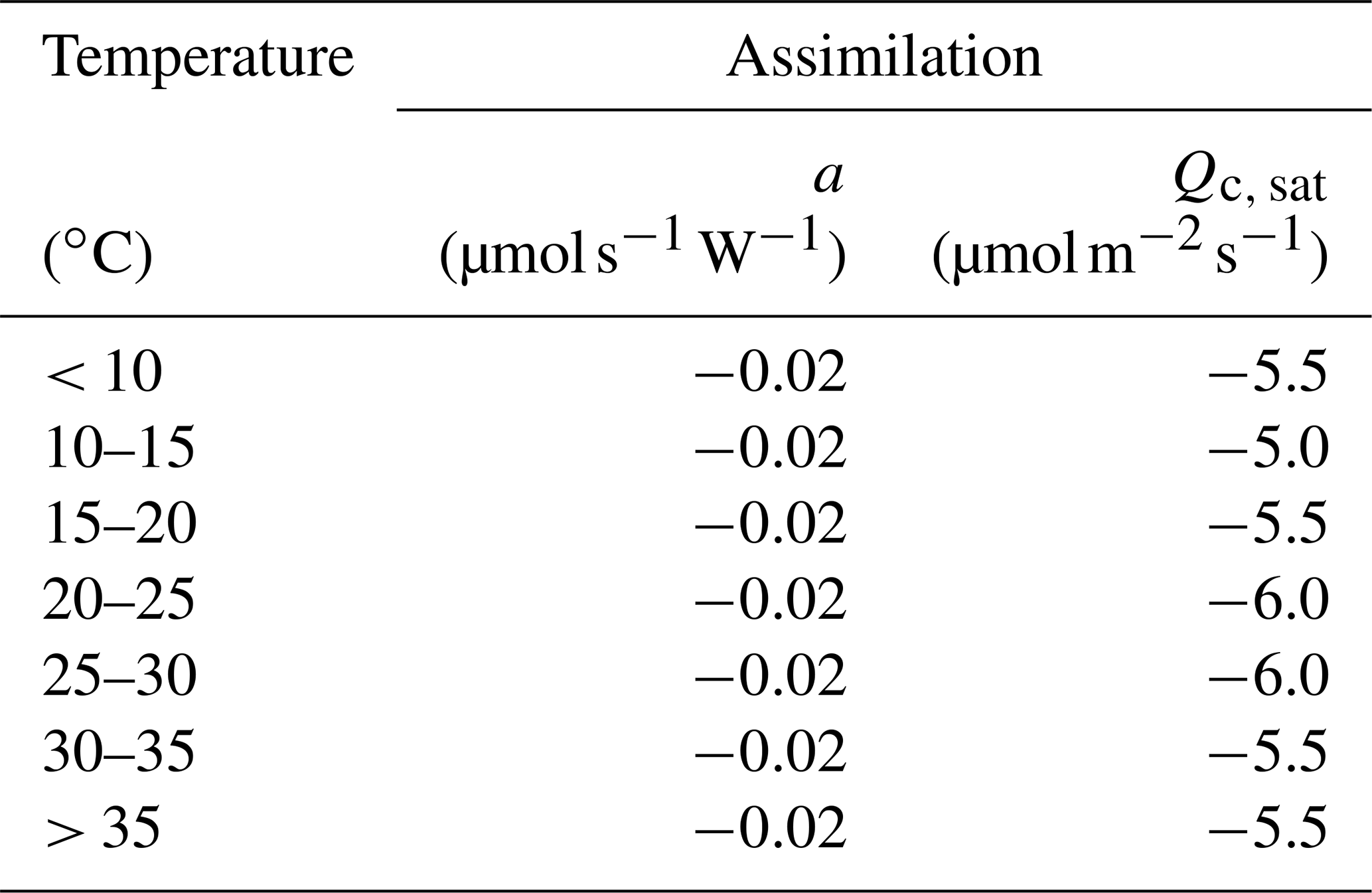
According to Falge et al. (2001b) and Hollinger et al. (1994), the factor a in Eq. (2) is the linear slope of the assimilation function beginning for a global radiation of 0 W m⁻² and analog for this modified net radiation. The slope of the assimilation function, a, and the assimilation at radiation saturation, Q_c, sat, were determined for 5 K binned classes for a data set with a footprint > 80 % from the pine area and data quality classes 1–6. The results of this parameterization are summarized in Table 2.

2.4.4 Generation of the final data set for cumulative fluxes

The flow chart of data processing for the generation of the final data set is shown in Figs. S2 and S3. Missing data as well as data with quality flag 9, together amounting to 5 % of the entire data set, were replaced with estimates computed using the Lloyd–Taylor and Michaelis–Menten functions, following the parameterizations detailed in the two prevision sections. The same was done for another 5 % of the entire data set, comprising the data that did not pass the spike test that was applied to the data with quality flags 1 to 8. The nighttime period – during which assimilation was assumed to be zero and, hence, just the Lloyd–Taylor function was applied to estimate NEE – was defined as the time between 15 min before sunset and 15 min after sunrise because global radiation was not measured. Gap filling of 238 daytime 30 min records was hampered by missing net radiation data, so they were substituted with interpolated values. The same was done for the 473 estimates from gap filling that did not pass a second spike test. For periods up to 5 h, interpolated values were calculated by linear interpolation between the two values immediately before and immediately after the period; for longer periods, they were computed per time-of-the-day 30 min intervals, as the average of the values of the 15 preceding and 15 succeeding days. This procedure allowed the replacement of only 10 % of measured data with values estimated by gap filling. The application of a typical u_∗ threshold as 0.28 m s⁻¹ (Wutzeler et al., 2018) would have resulted in the replacement of almost 50 % of the measured data. The replacement of only 10 % of the data was particularly relevant due to the difficulties encountered in the parameterization of the gap-filling equations (see Sect. 2.4), which in turn could be attributed to the short study period and its dynamic (a)biotic conditions. The present procedure did not involve a selection according to the footprint because the CO₂ fluxes from the burnt pine forest appeared to be identical to those from the burnt eucalypt patches to the east of the flux tower (see Sect. 3.1.3).

2.5 Ground heat flux

The ground heat flux was calculated from the abovementioned soil temperature measurements (Table 1) and the heat storage of the topsoil, from the soil surface to a depth of 15 cm (Liebethal and Foken, 2007; Yang and Wang, 2008):

$$\begin{array}{}\text{(5)}& Q_{\mathrm{G}}\left(\mathrm{0}\right)=-\mathit{\lambda }{\left.{\displaystyle \frac{\partial T}{\partial z}}\right|}_{z=-\mathrm{0.15}}+\underset{-\mathrm{0.15}}{\overset{\mathrm{0}}{\int }}{c}_{\mathrm{v}}\left(z\right)T_{\mathrm{s}}\left(z\right)\mathrm{d}z,\end{array}$$

where T_s is the soil temperature, z is the depth, λ is the thermal molecular conductivity of the soil and c_v is the soil's volumetric heat capacity. The accuracy of this method is comparable to that using heat flux plates (Liebethal et al., 2005). The soil temperature at 15 cm depth was calculated as the average of the temperatures at 10 and 20 cm depth, while the thermal conductivity was estimated as the mean value at the same depth, using the temperature-dependent data given by Hillel (1998). The heat capacity was computed using the equation proposed by de Vries (1963), ignoring the organic soil component:

$$\begin{array}{}\text{(6)}& c_{\mathrm{v}}=c_{\text{v,m}}{x}_{\mathrm{m}}+c_{\text{v,w}}\mathit{\theta },\end{array}$$

where θ is the soil volumetric water content; c_v,m and c_v,w are the heat capacities of the mineral soil compounds (1.9 × 10⁶ $\mathrm{J}{\mathrm{m}}^{-\mathrm{3}}{\mathrm{K}}^{-\mathrm{1}}$) and soil water (4.0 × 10⁶ $\mathrm{J}{\mathrm{m}}^{-\mathrm{3}}{\mathrm{K}}^{-\mathrm{1}}$), respectively; and x_m is the bulk density of the mineral compounds (0.566 m³ m⁻³), which was estimated from dry bulk density measurements of the soil and an assumed particle density of the mineral soil of 2650 kg m⁻³.

2.6 Soil volumetric water content classes

Table 3 Classes of soil volumetric water content (VWC) at 2.5 cm depth, where θ_max is the maximum of the 30 min median values observed during the first hydrological year.

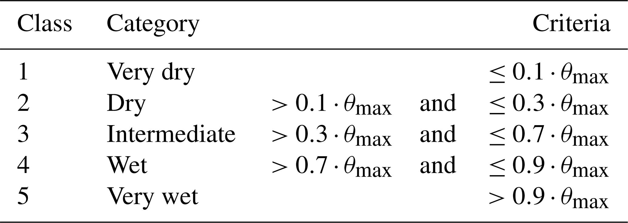
The 30 min values of soil volumetric water content (VWC) of each of the five inter-patch sensors along the transect were first rescaled to a zero-minimum value. This was done by summing the negative minimum value over the first post-fire hydrological year (ranging from −0.07 to −0.01 m³ m⁻³) or, in one case, subtracting the positive minimum value (0.01). The median of the rescaled values of the five sensors was then calculated for each timestamp (Fig. S4). These 30 min median values were subsequently divided, somewhat arbitrarily, into five classes (Table 3).

Figure 8 Volumetric water content (VWC) classes of the topsoil (from dry, Eq. 1, to wet, Eq. 5, as defined in Table 2) during the hydrological year 2017–2018. The corresponding 30 min VWC values are in Fig. S4.

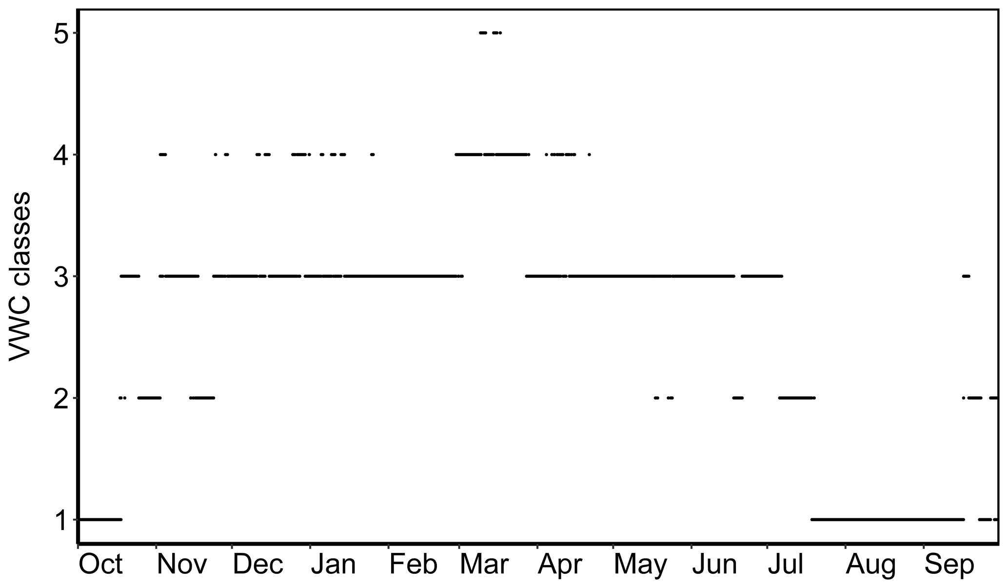
The temporal pattern of the five VWC classes during the first post-fire year is shown in Fig. 8, while the corresponding pattern of the 30 min median VWC values is given in Fig. S7 in the Supplement. The driest soil conditions (classes 1 and 2) prevailed during the initial and final periods of this study, from October to November 2017 and from July to October 2018, while the wettest conditions (class 5) only occurred occasionally, during March 2018 following intense rainfall (see Fig. S8 in the Supplement).

3 Results and specific discussion

3.1 Selected cases

Five 3–6 d periods with good footprint conditions were selected to illustrate distinct flux conditions that were identified during the first post-fire hydrological year (including the first measurement days during September 2017).

3.1.1 The role of dew formation

The period from 26 to 29 September 2017, immediately after the tower became operational, was selected for revealing the role of dew formation on NEE fluxes (Figs. S9 and S10 in the Supplement). By then, no rainfall had occurred after the wildfire (Fig. S8), and the topsoil was very dry (Fig. 8). During this period, the sky was mostly clear; the sensible heat flux was of the same order as the net radiation; and the maritime pine stands generally comprised more than 60 % of the footprint area. The fluxes of both CO₂ and NEE (including storage term) were about zero during nighttime and showed an uptake up to −5 $\mathrm{\mu }\mathrm{mol}{\mathrm{m}}^{-\mathrm{2}}{\mathrm{s}}^{-\mathrm{1}}$ during daytime. A substantial emission of CO₂ only occurred around sunrise on 28 September 2017, when the relative humidity at the top of the flux tower reached 80 %–90 % and dew formation took place. The occurrence of dew formation can be inferred from relative humidity in combination with sensible and latent heat fluxes. Dew formation simultaneously produces a positive, upward sensible heat flux due to the heat of condensation and a negative, downward latent heat flux, while the subsequent evaporation of the dew produces fluxes of the opposite signs. Worth noting, however, is that the observed latent heat fluxes were always below the detection limit of ± 10 W m⁻² (Mauder et al., 2006) during the early-morning hours, reflecting the very dry soil conditions.

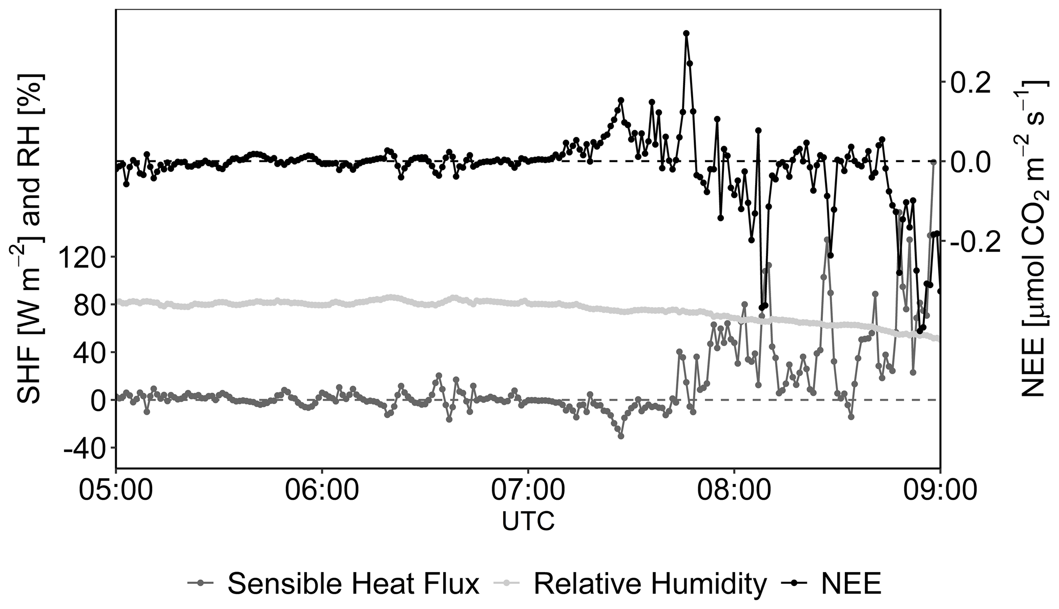
Figure 9 Relative humidity (RH) and sensible heat (SHF) and NEE fluxes with a 1 min resolution during the morning hours of 28 September 2017, indicating dew formation followed by evaporation of dew and associated CO₂ emission between 06:30 and 07:30 UTC.

The suggestion that the positive NEE flux during the early morning of 28 September 2017 was triggered by dew formation was further analyzed by calculating the NEE fluxes with a 1 min time resolution, using the wavelet method (Sect. 2.3.4), and comparing them with the relative humidity and the sensible heat fluxes with the same time resolution (Fig. 9). The WPL correction (Webb et al., 1980) was not applied because it would be very small under the specific conditions and, therefore, would not have noticeably changed the CO₂ fluxes.

As shown in Fig. 9, relative humidity was about 80 % at the top of the flux tower during the early-nighttime hours of 28 September 2017 and presumably close to 100 % near the ground because of the clear sky and associated temperature gradient. There were recorded fluctuations in relative humidity related to fluctuations in sensible heat fluxes and CO₂ fluxes. Before 06:00 UTC, however, both fluxes were below their respective detection limits. At around 06:30 UTC, on the other hand, relative humidity increased to 85 %, and this increase was associated with sensible heat fluxes of up to 20 W m⁻², clearly in line with the occurrence of dew formation. After 07:00 UTC, relative humidity decreased again to below 80 %, creating conditions for the evaporation of the dew. This dew evaporation was also indicated by negative sensible heat fluxes of up to −30 W m⁻² between 07:15 and 07:30 UTC because the evaporation process requires energy. In turn, this peak in negative sensible heat fluxes was accompanied by a peak in upward CO₂ fluxes, suggesting that the upward water vapor flux worked as a kind of a pump for CO₂ emissions.

3.1.2 The role of the first rainfall events after the wildfire

The first post-fire rainfall events occurred more than 2 months after the wildfire, between 17 to 22 October 2017, and significantly increased soil VWC (Figs. S7 and S8). The bulk of this rainfall occurred during the night from 17 to 18 October 2017 (8.4 mm) and around noon on 20 October 2017 (3.2 mm). During this 6 d period, the footprint area generally consisted of more than 80 % of the maritime pine stands; cloudy conditions prevailed (in spite of sunny periods on 17, 18 and 22 October 2017); and the latent heat flux contributed markedly to the energy exchange (Bowen ratio of about 1; Fig. S11 in the Supplement) because of the high relative humidity (exceeding 90 % during rainfall). With the onset of the autumn rainfall, the ecosystem started to be a source of CO₂, but the fluxes decreased again on 22 October 2017. Worth noting was that the second, smaller rainfall event of 20 October 2017 seemed to have a greater impact on CO₂ emissions than the first event of 17 and 18 October 2017. The large scatter in NEE fluxes observed during some periods could be explained by conditions of low turbulence and the generally low fluxes.

Figure 10 Cumulative NEE fluxes and 30 min rainfall during the initial window of disturbance, from 1 October to 31 December 2017.

The role of rainfall periods in NEE fluxes during the initial post-fire window of disturbance was also evidenced by the cumulative NEE values from 1 October to 31 December 2017 (Fig. 10). After an initial period of net assimilation, three marked peaks in net CO₂ emissions occurred that were associated with periods of intense rainfall during mid-October and early and late November 2017. By contrast, intense rainfall periods during early and especially also late December 2017 only had minor impacts on net CO₂ emissions. This was probably due to the lower temperatures, ranging from 5 to 15 ^∘C during daytime.

3.1.3 The role of woodland type and (antecedent) rainfall during summer conditions

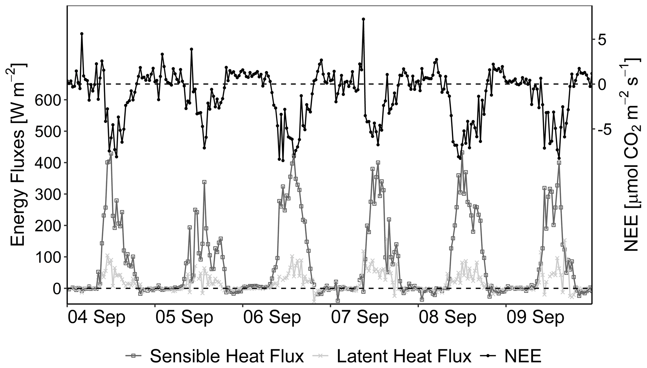
Figure 11 Energy and NEE fluxes from the maritime pine stands during a rainless period towards the end of the first post-fire hydrological year, from 4 to 9 September 2018.

Energy and NEE fluxes from the maritime pine stands under dry conditions during the first post-fire summer are illustrated in Fig. 11. During the selected, rainless 6 d period from 4 to 9 September 2018, the footprint area generally consisted of more than 80 % of the pine stands, while topsoil VWC was consistently very dry (class 1; Fig. 8), reflecting the less than 1 mm of antecedent rainfall over the preceding 4-week period (Fig. S8).

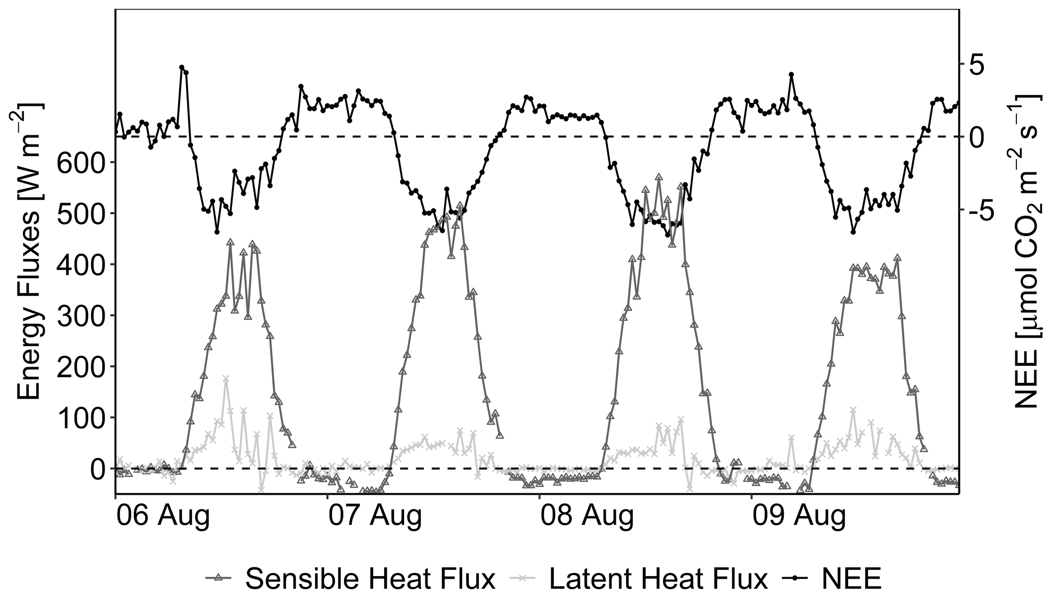
Figure 12 Daily cycles of 30 min sensible and latent heat fluxes and NEE fluxes during a rainless period in midsummer, from 6 to 9 August 2018, when these fluxes originated from the eucalypt patches.

A second rainless summer 2018 period was selected to analyze energy and NEE fluxes from the eucalypt patches located to the east of the tower. Even though this 4 d period was about 1 month earlier, from 6 to 9 August 2018, topsoil VWC was equally very dry, and antecedent rainfall over the preceding 4-week period was equally less than 1 mm. NEE fluxes under summer 2018 conditions did not differ conspicuously between the eucalypt (Fig. 12) and maritime pine stands (Fig. 11), neither in terms of diurnal patterns nor in terms of measured values. As to be expected, sensible heat fluxes did differ markedly, being clearly higher during early August than early September. The same was true for the Bowen ratio, attaining an average value as high as 5.4 over the 6–9 August 2018 period, as opposed to 2.7 over the 4–9 September 2018 period.

A 3 d period during early July 2018 was selected to examine how summer 2018 NEE fluxes from the maritime pine stands (comprising > 80 % of the footprint area) were affected by (antecedent) rainfall (Fig. S12 in the Supplement). Two minor rainfall events (defined here as periods that were preceded and succeeded by at least 3 h without rainfall) occurred on 1 July 2018. The first one started at 21:00 UTC on 30 June and ended at 02:30 UTC on 1 July and amounted to 2.0 mm, and the second lasted from 14:00 to 15:30 UTC on 1 July and amounted to 0.4 mm (Fig. S8). These rainfall events lead to a minor increase in topsoil VWC (Fig. S7). Arguably, the main contrast with early September was the antecedent rainfall, amounting to 40.3 mm as opposed to 0.1 mm over the preceding 14 d. This contrast was also reflected in topsoil moisture conditions, which were moderate (VWC class) during early July as opposed to very dry (VWC class 1) during early September. The NEE fluxes during early July, however, did not differ markedly from those of early September. Apparently, neither assimilation nor respiration processes suffered from serious moisture limitations by early September, in spite of the very dry conditions of the topsoil.

3.2 Cumulative carbon dioxide fluxes

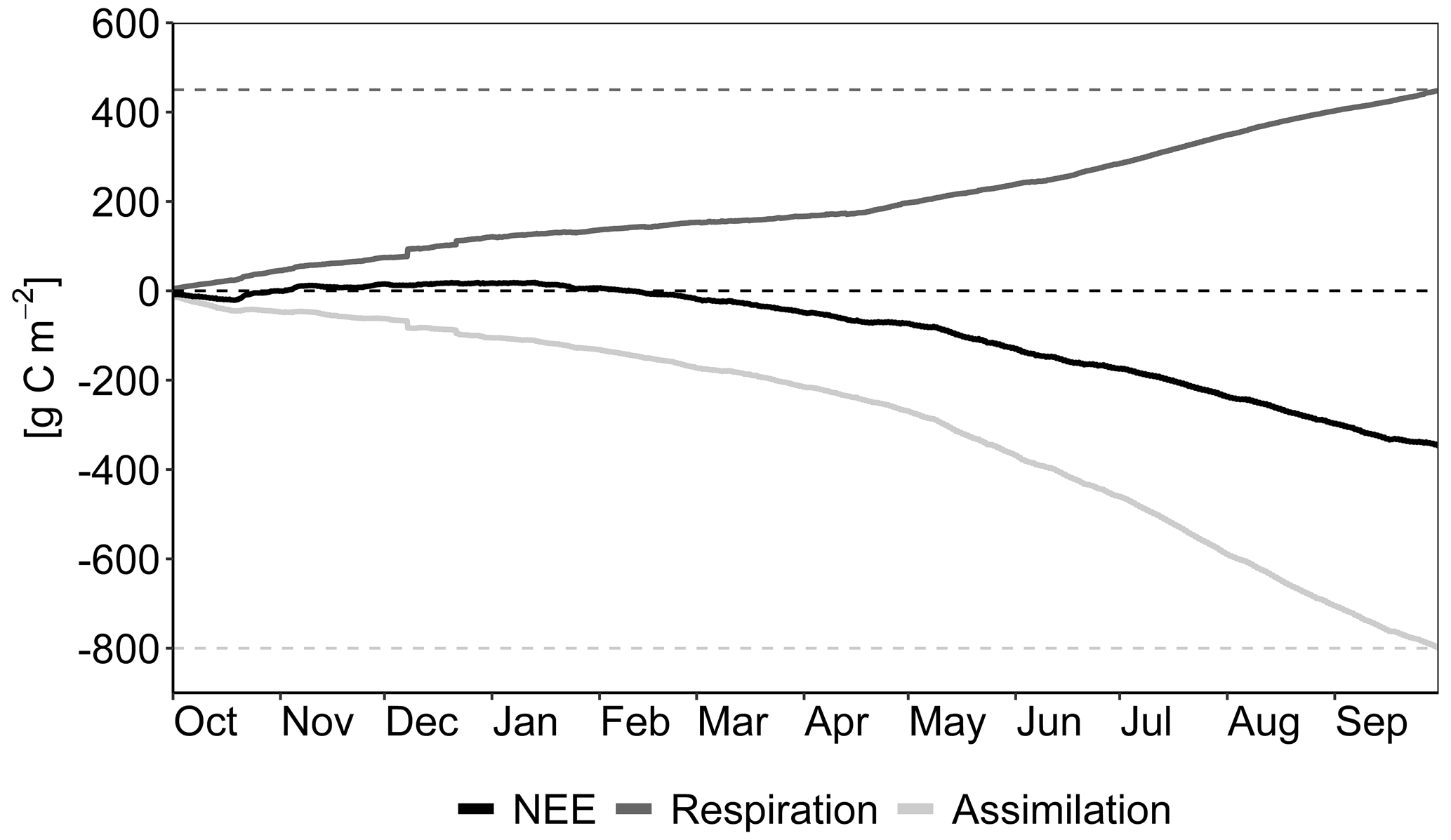
Figure 13 Cumulative NEE, assimilation and respiration fluxes during the first hydrological year after wildfire, from 1 October 2017 to 30 September 2018.

The cumulative CO₂ fluxes over the first hydrological year following the wildfire (1 October 2017–30 September 2018) are shown in Fig. 13. No distinction was made between the fluxes from the maritime pine stands and those from the eucalypt stands for two reasons: first, because the pine-stand fluxes were predominant, given the prevailing west-northwesterly to northerly wind directions, and second, because the fluxes from the two forest types appeared to be similar during summer 2018 (Sect. 3.1.3). In terms of NEE patterns, five different periods could be distinguished during this first post-fire year. During the immediate post-fire period, which ended with the first rainfall event on 17 October 2017, the burnt area acted as a carbon sink, even if just a small one. During the ensuing period, which ended in mid-December 2017, the burnt area functioned as a carbon source, especially following periods of intense rainfall. During the coldest period from mid-December 2017 until the end of January 2018, NEE fluxes were close to zero. With the onset of warmer temperatures during early February 2018, followed by a (practically) rainless February, the area started to become a small carbon sink. This period continued during the next 2 rainiest months, during which short intervals occurred when respiration was the dominant process. Finally, from May 2018 onwards, the area was a marked carbon sink, with assimilation clearly prevailing over respiration.

The cumulative assimilation over the first post-fire hydrological year was roughly twice the cumulative respiration. This was remarkable, since forest carbon flux studies have generally been found both to be of the same order of magnitude (e.g., Luyssaert et al., 2010). This discrepancy between assimilation and respiration resulted to a large extent from the last of the five abovementioned periods, starting in May 2018. A possible reason for the discrepancy was the impossibility of parameterizing respiration under intermediate and wet soil conditions, and, hence, that respiration was possibly underestimated. However, the amount of gap-filled data was very low.

4 Overall discussion

The following discussion focuses on the three main novelties of this study, due also to the lack of comparable EC studies of ecosystem recovery during the initial stages following wildfire.

4.1 Data analysis

The present data set was less suited for the standard procedure of data quality assessment using a threshold of friction velocity (Goulden et al., 1996) and, hence, standardized data analysis routines as used in networks such as ICOS (Integrated Carbon Observation System) and NEON (National Ecological Observatory Network; Metzger et al., 2019; Rebmann et al., 2018). NEE fluxes tended to be very low during the first year after the wildfire, and wind speeds were generally low, not exceeding 3 m s⁻¹. To address these particular conditions, a specific procedure was developed in the present study, based on data quality flagging (Ruppert et al., 2006). It allowed for limiting the need for gap filling to about 5 % of the data, while gap filling of up to 30 % of the data is common for the fractional-velocity-based procedures. The present procedure, however, required thorough data analysis, involving not only repeated MAD and spike tests and modeling of the footprint area but also assessing the possible influence of the standing burnt tree trunks on mechanical turbulence. Furthermore, an exploratory analysis of the closure of the energy balance was carried out because amongst other reasons ground heat fluxes were not measured directly in this study. The energy balance closure proved acceptable, not raising major concerns about the correctness of the measured carbon fluxes. In addition, the Bowen ratio was typically in the range of 1 to 5, thereby guaranteeing that the gaps in energy balance closure did not markedly influence the carbon fluxes and that these fluxes did not require correction for such gaps (Charuchittipan et al., 2014). Gap filling itself was based on careful parameterization of the Lloyd–Taylor function, in particular by taking into account soil moisture as a key factor in the respiration of Mediterranean and dry ecosystems (Richardson et al., 2006; Sun et al., 2016). The nighttime NEE data also revealed this importance of soil moisture but only allowed for a reliable parameterization of the Lloyd–Taylor function for very dry to dry soil moisture conditions and not for intermediate to wet conditions. The latter could be due to the fact that these intermediate and wet conditions included three of the five periods that were distinguished in terms of NEE fluxes (Sect. 3.2), with fluxes ranging from practically zero during early winter (mid-December 2017 to end of January 2018) to their highest values during late spring (May to June 2018). Finally, the potential of the wavelet method as a complementary tool to analyze specific short-term events with an elevated temporal resolution was demonstrated, as it provided crucial insights into CO₂ fluxes during and following dew formation. The diurnal pattern in NEE fluxes was similar to the average monthly trends reported by Serrano-Ortiz et al. (2011) for a pine stand that had burned 4 years earlier and had not been intervened afterwards. This was particularly the case for the June fluxes of Serrano-Ortiz et al. (2011) because of their greater contrast between daytime and nighttime fluxes.

4.2 Respiration fluxes upon wetting by dew formation

Dew formation has been reported for many climate types, affecting, amongst others, microbial activity during rainless periods (Agam and Berliner, 2006; Gliksman et al., 2018; Verhoef et al., 2006). To the best knowledge of the authors, dew formation had not yet been observed in burnt areas. Its impact on ecosystem respiration differed fundamentally from the Birch effect that Sánchez-García et al. (2020) observed in the same burnt area as studied here and equally before the occurrence of post-fire rainfall (i.e., on 17 October 2017 in the case of the site with wildfire ash). Sánchez-García et al. (2020) reported the highest soil effluxes immediately after stopping the simulated rainfall (after 10 min) but inferred, based on wetting experiments with the same soils under laboratory conditions, that peak values had occurred even earlier. The short duration of the peak was argued to suggest that the Birch effect resulted from the displacement of CO₂-rich air in soil and especially ash pores by infiltrating water (degassing) because of amongst other reasons the likely suppression of microbial activity due to the still recent sterilization by the fire. For the same reasons, the dew-induced CO₂ efflux observed in this study was probably due to a physical process rather than to a microbial activity. This process, however, differed from the displacement of ash–soil air by infiltrating water in the sense that the respiration flux only started some half an hour after the dew formation, with the onset of the evaporation of the dew. The observed water vapor flow from the soil surface was large enough to generate a pumping effect with vertical wind velocities at the surface in the order of 10⁻⁴ m s⁻¹ (Webb et al., 1980), on the one hand, and, on the other, the amount of dew was sufficient to explain the CO₂ efflux between 07:01 and 07:41 UTC. This CO₂ efflux amounted to 4.94 mg m⁻² or 2.50 cm³ m⁻². The sensible heat flux during this 40 min period was 17.3 × 10³ J m⁻², i.e., involving enough energy to evaporate the 7.03 g m⁻² or 7.02 cm³ m⁻² of dew, which, in turn, is equivalent to 0.41 m³ m⁻² of CO₂ gas (see Foken et al. (2021) for the temperature-dependent physical parameters). The occurrence of this pumping effect rather than the degassing effect observed by Sánchez-García et al. (2020) was probably due to the comparatively small amount of dew water (0.007 vs. 25 mm of simulated rain), combined with the presence of a considerable wildfire ash layer. The inter-patch ash load determined at the five transect points on 7 September 2017 averaged 2.21 g m⁻², with a minimum of 762 g m⁻². This ash layer will have easily absorbed the small amount of dew water, as wildfire ash has an elevated water storage capacity (Balfour and Woods, 2013; Leighton-Boyce et al., 2007). Probably, the wetting of the ash layer was limited to its immediate surface, not causing significant degassing of ash pores underneath. This wetting might have created a kind of a seal, even if perhaps a spatially heterogeneous one, as Sánchez-García et al. (2020) reported that almost 50 % of the pine ash was severely to extremely water repellent. The subsequent evaporation would then have broken this seal and/or simply pumped out part of the CO₂ stored in the underlying ash pores. Further research is need to clarify to which extent the emitted CO₂ originated from a rapid restoration of microbial respiration caused by microbial biomass growth and the activation of extracellular enzymes, as has been observed after the first post-fire rainfall events (Fraser et al., 2016; Waring and Powers, 2016).

4.3 Cumulative NEE fluxes

The discussion of the cumulative NEE fluxes of this study is seriously hampered by the limited number of post-fire EC studies and, in particular, by the existence of just one prior EC study that monitored a large part of the first post-fire year (Table S1). This latter study, of Sun et al. (2016), found that a eucalypt woodland in southern Australia was a net carbon source for a considerably longer post-fire period than the present site, i.e., until the 15th instead of the 5th month after fire. This delay could be due to the much drier, semi-arid climate conditions together with low soil nutrient availability, resulting in a reduced pre-fire NEP (net ecosystem production; < 100 $\mathrm{g}\mathrm{C}{\mathrm{m}}^{-\mathrm{2}}{\mathrm{yr}}^{-\mathrm{1}}$) of the patchy, low-stature vegetation. The net carbon emissions during the first 3 monitoring months of Sun et al. (2016), however, did not differ widely from the cumulative NEE fluxes observed in this study over the 2 months following the first post-fire rainfall events (mid-October to mid-December 2017). The former ranged from 11 to 19 g C m⁻²  per  month for post-fire months 4 to 6, whereas the latter averaged about 20 g C m⁻²  per  month. The other post-fire EC studies suggested that re-establishment of the carbon sink function after fire took at least 1 to 9 years (Amiro et al., 2006: > 1 year; Dadi et al., 2015: > 2 years; Serrano-Ortiz et al., 2011: < 4 years; Mkhabela et al., 2009: > 6 years; Dore et al., 2008: > 9 years).

Comparison of the cumulative annual NEE flux of this study with those of prior EC studies in burnt woodlands and/or unburnt pine areas (summarized in Tables S1 and S2) showed that the present cumulative NEE of −290 $\mathrm{g}\mathrm{C}{\mathrm{m}}^{-\mathrm{2}}{\mathrm{yr}}^{-\mathrm{1}}$ over the first post-fire year differed least from that reported by Moreaux et al. (2011) for their 4-year-old maritime pine plot (−243 $\mathrm{g}\mathrm{C}{\mathrm{m}}^{-\mathrm{2}}{\mathrm{yr}}^{-\mathrm{1}}$). The annual NEE of a second, intervened plot studied by Moreaux et al. (2011), however, was much lower (−65 $\mathrm{g}\mathrm{C}{\mathrm{m}}^{-\mathrm{2}}{\mathrm{yr}}^{-\mathrm{1}}$). The authors attributed this to the rapid growth of shrubs and herbaceous species following the weeding and thinning, possibly even compensating a decrease in GPP (gross primary production) by the pines due to the thinning. This intervened plot had also been studied earlier by Kowalski et al. (2003), showing that the undergrowth species started fixating carbon just a few months after the clear cutting of the original 50-year-old maritime pine stand. Shrub species should also explain the bulk of the GPP at the present site, as their median cover at the five transect points by mid-September 2018 summed 50 % as opposed to 3 % and 2 % for herbaceous and tree species, respectively (Table S2).

Even more unexpected than the rapid recovery of the carbon sink function at the present site was the net carbon assimilation observed during the immediate post-fire period, until the first post-fire rainfall events of mid-October 2017. The net assimilation was about 1.0 $\mathrm{g}\mathrm{C}{\mathrm{m}}^{-\mathrm{2}}{\mathrm{d}}^{-\mathrm{1}}$, i.e., between the rates during the other two periods with net assimilation (February–April 2018: 0.6 $\mathrm{g}\mathrm{C}{\mathrm{m}}^{-\mathrm{2}}{\mathrm{d}}^{-\mathrm{1}}$; May–October 2018: 1.8 $\mathrm{g}\mathrm{C}{\mathrm{m}}^{-\mathrm{2}}{\mathrm{d}}^{-\mathrm{1}}$). Unlike the two assimilation periods from early 2018 onwards, this 2017 assimilation period was difficult to link to the recovery of the understory vegetation for two main reasons: (i) the understory vegetation was fully consumed by the fire, and (ii) the recovery of the understory vegetation was still very reduced by early January, as illustrated for three key resprouter shrub species in Fig. S13 in the Supplement. Possibly, this immediate post-fire photosynthetic activity originated from the various patches of pines with scorched crowns immediately next to the EC tower as well as at larger distance to the south and west of it, as shown in Fig. S1b. An alternative explanation would be resprouting eucalypts, in particular the four individual trees near the tower and/or the patch to the east of it, as eucalypts tend to resprout relatively quickly and vigorously after fire.

5 Conclusions

The main conclusion of this first study into CO₂ fluxes following wildfire over the first post-fire hydrological year were the following:

• i.

  A specific data analysis procedure including data quality flagging, MAD and spike testing, footprint analysis, soil-moisture-dependent gap filling, and assessment of mechanical turbulence had to be developed because of the very low fluxes and prevailing wind speeds below 3 m s⁻¹ but which allowed for reducing the need for gap filling to just about 5 % of the data.

• ii.

  The use of the wavelet method for the determination of turbulent fluxes with a 1 min time resolution proved to be extremely helpful for a detailed analysis of the role of dew formation on soil respiration.

• iii.

  The cumulative NEE fluxes during the first hydrological year after a wildfire that occurred in August 2017 revealed an intricate temporal pattern that could be divided into five phases. The first phase (first half of October 2017) and the last two phases (from early February 2018 onwards) were (mainly) governed by assimilation; the second (mid-October to mid-December 2017) was dominated by soil respiration that was closely linked to the first post-fire rainfall events; and the third phase (mid-December 2017 to early February 2018) had negligible fluxes.

• iv.

  The carbon sink function of this maritime-pine-dominated area was re-established within less than half a year after the wildfire, mainly due to the recovery of the understory vegetation of both resprouter and seeder species.

• v.

  Dew formation during the rainless, immediate post-fire period produced a noticeable soil carbon efflux that was linked to dew evaporation and not to instantaneous degassing due to wetting.