the Creative Commons Attribution 4.0 License.
the Creative Commons Attribution 4.0 License.
 | 17 Jun 2021
The fate of upwelled nitrate off Peru shaped by submesoscale filaments and fronts
Jaard Hauschildt
Soeren Thomsen
Vincent Echevin
Andreas Oschlies
Yonss Saranga José
Gerd Krahmann
Laura A. Bristow
Gaute Lavik
Filaments and fronts play a crucial role for a net offshore and downward nutrient transport in Eastern Boundary Upwelling Systems (EBUSs) and thereby reduce regional primary production. Most studies on this topic are based on either observations or model simulations, but only seldom are both approaches are combined quantitatively to assess the importance of filaments for primary production and nutrient transport. Here we combine targeted interdisciplinary shipboard observations of a cold filament off Peru with submesoscale-permitting (∘) coupled physical (Coastal and Regional Ocean Community model, CROCO) and biogeochemical (Pelagic Interaction Scheme for Carbon and Ecosystem Studies, PISCES) model simulations to (i) evaluate the model simulations in detail, including the timescales of biogeochemical modification of the newly upwelled water, and (ii) quantify the net effect of submesoscale fronts and filaments on primary production in the Peruvian upwelling system. The observed filament contains relatively cold, fresh, and nutrient-rich waters originating in the coastal upwelling. Enhanced nitrate concentrations and offshore velocities of up to 0.5 m s−1 within the filament suggest an offshore transport of nutrients. Surface chlorophyll in the filament is a factor of 4 lower than at the upwelling front, while surface primary production is a factor of 2 higher. The simulation exhibits filaments that are similar in horizontal and vertical scale compared to the observed filament. Nitrate concentrations and primary production within filaments in the model are comparable to observations as well, justifying further analysis of nitrate uptake and subduction using the model. Virtual Lagrangian floats were released in the subsurface waters along the shelf and biogeochemical variables tracked along the trajectories of floats upwelled near the coast. In the submesoscale-permitting (∘) simulation, 43 % of upwelled floats and 40 % of upwelled nitrate are subducted within 20 d after upwelling, which corresponds to an increase in nitrate subduction compared to a mesoscale-resolving (∘) simulation by 14 %. Taking model biases into account, we give a best estimate for subduction of upwelled nitrate off Peru between 30 %– 40 %. Our results suggest that submesoscale processes further reduce primary production by amplifying the downward and offshore export of nutrients found in previous mesoscale studies, which are thus likely to underestimate the reduction in primary production due to eddy fluxes. Moreover, this downward and offshore transport could also enhance the export of fresh organic matter below the euphotic zone and thereby potentially stimulate microbial activity in regions of the upper offshore oxygen minimum zone.
- Article
(9781 KB) - Full-text XML
-
Supplement
(3209 KB) - BibTeX
- EndNote


The eastern margins of the subtropical oceans are characterized by upwelling of cold and nutrient-rich subsurface waters, caused by persistent along-shore winds that drive an offshore Ekman transport. The nutrients supplied to the sunlit surface ocean subsequently fuel high phytoplankton growth, which supports a rich ecosystem (Pennington et al., 2006). These Eastern Boundary Upwelling Systems (EBUSs) are found in all major ocean basins and are named after the Canary, Benguela, California, and Peru–Chile current systems. The Peru–Chile upwelling system (PCUS) is the most productive EBUS in the global ocean, accounting for 10 % of the global fish catch while occupying only 0.1 % of the ocean surface (Chavez et al., 2008). The Peru upwelling ecosystem and the fisheries that depend on it have immense economical importance for the local population. Furthermore, the high productivity and export of organic matter and its subsequent remineralization at depth result in high rates of oxygen consumption (Kalvelage et al., 2015; Loginova et al., 2019). In combination with poor ventilation by sluggish currents, this leads to the presence of the shallowest and most intense oxygen minimum zone (OMZ) in the global ocean (Wyrtki, 1962; Paulmier et al., 2006; Karstensen et al., 2008; Stramma et al., 2010). Besides being regions of high productivity, EBUSs are also globally relevant as natural sources of greenhouse gases to the atmosphere such as N2O (Friederich et al., 2008; Arévalo-Martínez et al., 2015) and CO2 (Chavez et al., 2007; Gruber, 2015; Köhn et al., 2017; Brady et al., 2019).
Mesoscale eddies have in the past been assumed to generally enhance biological productivity in the open ocean by either exposing nutrient-rich subsurface water to the well-lit euphotic zone or by lateral advection of nutrients (Falkowski et al., 1991; Oschlies and Garçon, 1998; Oschlies, 2002). Conversely, in the highly productive EBUS, eddies and filaments have been shown to decrease productivity by exporting nutrients and organic matter offshore and downward below the euphotic zone (Rossi et al., 2008, 2009; Lathuilière et al., 2010; Gruber et al., 2011; Nagai et al., 2015). Such features are ubiquitous in the PCUS (Penven et al., 2005; Colas et al., 2012; Thomsen et al., 2016a, b; Pietri et al., 2013; McWilliams et al., 2009). As the upwelling front meanders and eventually becomes unstable, an ageostrophic secondary circulation develops in order to restore geostrophic balance (Thomas et al., 2008; McWilliams et al., 2009, 2015). This ageostrophic flow field can drive large vertical velocities and thus impact the physical–biogeochemical coupling by modifying vertical and lateral transports of nutrients and organic matter (Lapeyre and Klein, 2006; Lévy et al., 2012; Mahadevan, 2015). The downward fluxes can be understood as subduction of surface water along isopycnals.
Previous studies have attempted to quantify the fluxes of biogeochemical tracers related to eddies and filaments in EBUSs using biogeochemical models of various complexity (e.g., in the California EBUS – Nagai et al., 2015; in the PCUS – Frenger et al., 2018; Montes et al., 2014; Bettencourt et al., 2015; and José et al., 2017; in the Canary EBUS – Lovecchio et al., 2018; in the Benguela EBUS – Schmidt and Eggert, 2016). One aspect previous model studies have not addressed are the eddy fluxes of iron, a tracer which is known to play a role in limiting primary production in the PCUS (Hutchins et al., 2002; Bruland et al., 2005; Browning et al., 2018). Furthermore, most of these studies are purely based on models, and comparison to observations has proven difficult due to the difficulties of observing vertical velocities. Regional simulations are often primarily validated using surface chlorophyll maps derived from ocean color, which does not allow the resolution of the underlying physical (e.g., subduction) and biogeochemical processes (e.g., primary production, hereafter PP). When attempting to quantify the effect of subduction on biogeochemistry using models, we need to ensure that the timescales of PP and subduction are realistic: for instance, if the timescale of nitrate uptake by PP was shorter than the subduction timescale, more organic matter (produced in the surface layer) than nitrate would be subducted. If it was longer, the opposite would be true. When attempting to quantify the effect of subduction on biogeochemistry using models, we therefore need to ensure that the timescales of PP and subduction are realistic. Dedicated studies combining multi-disciplinary observations with modeling efforts at the meso- and submesoscale are key to advance our understanding of complex physical–biogeochemical interactions (Oschlies et al., 2018). Evaluating the models at these scales allows trust in the simulation of submesoscale processes to be gained to assess the associated uncertainties and possible systematic biases.
The degree to which dynamical processes of a certain scale are represented in a simulation depends on the effective horizontal resolution of the numerical model (Capet et al., 2008a; Soufflet et al., 2016). So far, coupled physical–biogeochemical model simulations focusing on eddy fluxes of biogeochemical tracers (e.g., Nagai et al., 2015, for the California EBUS) have been limited to a horizontal resolution of ∼ 5 km in mid-latitudes, which is not sufficient to represent submesoscale dynamics as the effective resolution of a model is much lower due to strong kinetic-energy dissipation at the smallest resolved scales (Soufflet et al., 2016). Various purely physical model simulations (Capet et al., 2008b; Colas et al., 2012) and idealized biogeochemical simulations (Lathuilière et al., 2010) suggest that an increase in the horizontal resolution leads to further enhancement of horizontal and vertical fluxes.
In this study, we focus on filaments and fronts which constitute the upper end of the submesoscale variability spectrum with length scales of 𝒪(1–10) km (McWilliams, 2016). A quantification of the net effect of filaments and submesoscale frontal processes on the offshore and downward nutrient transport and PP off Peru is missing so far. Therefore, we address the following questions:
-
What is the fate of the upwelled nitrate? In particular, what is the amount of nitrate subduction, and how does it impact PP?
-
What is the impact of horizontal model resolution on subduction and PP?
To address these questions, we evaluate the model based on physical and biogeochemical observations of a cold filament. To assess the timescale of phytoplankton growth in our model, we will compare PP and nutrient concentrations in a modeled filament with observational data. Then, we will quantify how much of the upwelled nitrate off Peru is subducted below the euphotic zone without being utilized by biology.
This paper is structured as follows: in Sect. 2 the filament survey, the coupled physical–biogeochemical model, and all other data sources as well as analysis methods are described. In Sect. 2.8 the model performance with respect to the relevant physical and biogeochemical quantities and their horizontal variability is evaluated. In Sect. 3.1 and 3.2 the mean horizontal variability in the upwelling structure and cold filaments is characterized in detail in both observations and model simulations. In Sect. 3.3 the simulation is used to analyze pathways and timescales of nitrate export, subduction, and uptake and to compare model results against estimates from observations. In Sect. 3.4 the effect of submesoscale-permitting vs. mesoscale model resolution with respect to the simulated mean biogeochemical tracer fields is analyzed. Finally, the results are discussed in the context of the existing literature in Sect. 4, which also includes a detailed discussion of the limitations of our approach. Concluding remarks follow in Sect. 5.
2.1 Filament survey
A survey designed to investigate the biophysical coupling at a cold filament near 14∘ S off the coast of Peru was carried out on 12–17 April 2017 using an adaptive sampling strategy guided by real-time satellite images. The fieldwork was conducted during R/V Meteor cruise M136, which started on 11 April and ended on 29 April 2017 in Callao, Peru (Dengler and Sommer, 2017; Lüdke et al., 2020). The measurements were carried out in the framework of the interdisciplinary collaborative research center SFB 754 “Climate–Biogeochemistry Interactions in the Tropical Ocean” funded by the Deutsche Forschungsgemeinschaft (DFG). The cruise track during the survey consisted of five transects (Fig. 1a). The first transect (CROSS) mapped the upwelling region in the cross-shore direction with conductivity, temperature, and depth (CTD) measurements, including biogeochemical parameters (O2, NO, NO, NH) determined from water samples. On subsequent along-shore transects, a cold filament present ∼ 100 km southeast of transect CROSS was crossed by R/V Meteor four times in a zigzag pattern: twice with high-resolution underway CTD measurements of physical parameters heading in a southeast direction (PHY, PHY2) and two more times with station-based lowered CTD measurements including biogeochemical parameters heading in a northwest direction (BIO, BIO2). A dense sampling strategy with 8–10 km horizontal spacing between stations and 5–10 m vertical spacing between samples was applied on the biogeochemical transects. The physically underway transects (PHY, PHY2) were completed overnight in under 8 h, sampling with a horizontal spacing of under 1 km, similar to the resolution of the binned acoustic Doppler current profiler (ADCP) data. These physical data thus closely represent a synoptic view of the surface ocean. Sampling on the biogeochemical transects (BIO, BIO2) was done during daytime following each physical transect. Wind speed and direction on R/V Meteor were measured at 35.5 m height with a temporal resolution of 1 min and corrected to 10 m height following Smith (1988), similar to the procedure used by Köhn et al. (2017).
2.2 Oceanographic biophysical measurements
Hydrographic data were obtained from lowered conductivity, temperature, and pressure (CTD) measurements using a SeaBird SBE 9-plus CTD system equipped with two sets of pumped sensors. Water samples for oxygen, nutrients, and salinity were taken using 24 Niskin bottles (10 L) mounted on a General Oceanics rosette. Salinity samples were analyzed on board with a Guildline Autosal 8 model 8400B salinometer to calibrate conductivity measurements to practical salinity (PSS-78) with an uncertainty of 0.003 g kg−1. Practical salinity was converted to absolute salinity (TEOS-10) using routines of the Gibbs Seawater toolbox (https://github.com/TEOS-10/GSW-Python, last access: 7 September 2020). The CTD was also equipped with an oxygen sensor and a WET Labs (USA) fluorometer. The oxygen sensor was calibrated to an accuracy of 1.5 µmol using Winkler titration. As Winkler titration is not reliable in the core of the OMZ and tends to result in too high values (Revsbech et al., 2009; Kalvelage et al., 2013; Thomsen et al., 2016b), a concentration of 0 µmol L−1 was assumed in the core of the OMZ and the profiles corrected accordingly following Langdon (2010). To determine chlorophyll a concentrations from the measured chlorophyll fluorescence, the original factory calibration provided by the sensor manufacturer WET Labs (USA) was used. For more details on the calibration of chlorophyll fluorescence measurements, the reader is referred to Loginova et al. (2016). Underway subsurface temperature and salinity were measured using a Teledyne Oceanscience (Poway, USA) RapidCAST system acquiring profiles of the upper 70 m of the water column every 2 min, resulting in a horizontal resolution of 790 ± 240 m depending on the vessel speed. Subsurface current velocities on R/V Meteor were recorded by a vessel-mounted acoustic Doppler current profiler (vmADCP). The system used was a Teledyne RD Instruments OceanSurveyor 75 kHz ADCP capable of reaching a maximum depth of ∼ 700 m. The shallowest velocity measurements were acquired in a bin centered 18 m below the sea surface. During the filament crossing, the vessel speed was kept nearly constant at ∼ 5 m s−1 to obtain high-quality velocity measurements with a vertical resolution of 8 m and a horizontal resolution of 290 ± 26 m, which was subsequently averaged in 1 km bins. Nutrient concentrations were determined onboard by a QuAAtro autoanalyzer (SEAL Analytical, Southampton, UK) using standard photometric methods (Grasshoff et al., 1983).
During M136 a self-contained ultraviolet SUNA (submersible ultraviolet nitrate analyzer) nitrate sensor manufactured by Sea-Bird Scientific was attached to the CTD–rosette system similar to Alkire et al. (2010). SUNA sensors determine the concentration of nitrate by measuring the absorption of UV light over a fixed path length. The SUNA data have been reprocessed with the concurrent CTD pressure, temperature, and salinity (for bromide absorption) data to eliminate their effects on the absorption and the resulting nitrate concentrations (Sakamoto et al., 2009, 2017). The resulting SUNA nitrate concentrations have been extracted for the times at which bottles were closed on the water sampler. These concentrations have then been compared to the nitrate and nitrite concentrations measured with the autoanalyzer. SUNA nitrate values correlated highly with the autoanalyzer values (r squared: 0.9972, with the 10 % most deviating samples removed). SUNA values were also compared to the combined autoanalyzer concentrations of nitrate and nitrite, but the resulting correlation was somewhat weaker (r squared: 0.9964, with the 10 % most deviating samples removed). The SUNA measurements were thus corrected to match the nitrate (NO3) concentration by applying the following correction term, where NO3, old is the original measurement, and NO3, new is the final corrected value: NO. We applied this calibration to all SUNA nitrate concentrations.
All observational datasets mentioned above (Krahmann, 2018; Dengler et al., 2019a, b; Tanhua and Visbeck, 2018) are published at the world data center PANGAEA following the SFB 754 data policy (https://www.pangaea.de, last access: 1 December 2020; see “Code and data availability” section).
2.3 Incubations
Seawater samples were filled into 2 L polycarbonate bottles and were stored in the dark until tracer additions were made, which was always within 2 h of collection. Following the method outlined in Großkopf et al. (2012), incubations were started with the addition of sodium bicarbonate (NaH13CO3; >98 atom %, Sigma Aldrich) to yield a final enrichment of approximately 3.2 at. %. At each depth sampled, three bottles received a 13C addition, and a fourth bottle received no 13C and acted as an untreated control, allowing the natural abundance 13C to be determined at each depth. All bottles were placed into on-deck incubators with surface seawater flow-through and shaded with 20 %, 10 %, or 1 % surface irradiance (Lee Filters, Seattle, WA, USA), depending on the sampling depth. Incubations were terminated after 24 h by filtration onto 25 mm pre-combusted (450 ∘C, 4 h) GF/F filters (Whatman), which were dried onboard (50 ∘C, 12 h) and stored at room temperature until analysis. Prior to analysis, GF/F filters were acidified over fuming HCl overnight in a dessicator, dried, and pelletized in tin cups. Samples were analyzed for particulate organic carbon and isotopic composition using continuous-flow isotope ratio mass spectrometry coupled to an elemental analyzer. PP rates were calculated from the incorporation of 13C into biomass as described in Großkopf et al. (2012).
2.4 Data products
To guide the shipboard measurements and put them into a regional context, MODIS (Moderate Resolution Imaging Spectroradiometer) Level 2 along-track sea-surface temperature (SST) and chlorophyll a products with an approximate resolution of 1 km from the TERRA and AQUA satellites were used (https://oceandata.sci.gsfc.nasa.gov/, last access: 23 May 2017). We restricted our analysis to daylight images of SST and used the cloud mask based on ocean color because of obvious deficiencies of the cloud mask based on infrared SST data alone. SST data from AVHRR (Advanced Very High Resolution Radiometer; Saha et al., 2018) at 25 km resolution were provided by the NOAA (National Oceanic and Atmospheric Administration; ftp://eclipse.ncdc.noaa.gov/pub/OI-daily-v2/NetCDF/, last access: 1 December 2020). For evaluating the model performance with respect to PP, we used estimates of ocean net primary production (NPP) which were derived from both MODIS and SeaWIFS chlorophyll a using the Vertically Generalized Production Model (VGPM; Behrenfeld and Falkowski, 1997; http://sites.science.oregonstate.edu/ocean.productivity/, last access: 1 December 2020). Sea-surface height (SSH) data from DUACS/AVISO (Data Unification and Altimeter Combination System; Archiving, Validation and Interpretation of Satellite Oceanographic data) satellite altimeter product (SEALEVEL_GLO_PHY_L4_REP_OBSERVATIONS_008_047) used for model evaluation were produced and distributed at 0.25∘ resolution by the Copernicus Marine and Environment Monitoring Service (CMEMS; https://marine.copernicus.eu, last access: 1 December 2020). A global mixed-layer depth (MLD) climatology with resolution based on a 0.2 ∘C temperature criterion was provided by IFREMER (de Boyer Montégut et al., 2004; http://www.ifremer.fr/cerweb/deboyer/mld/Surface_Mixed_Layer_Depth.php, last access: 1 December 2020). Annual mean temperature and nitrate fields for model evaluation were provided at ∘ resolution by the CARS climatology (CSIRO Atlas of Regional Seas, Ridgway et al., 2002; http://www.marine.csiro.au/atlas/, last access: 1 December 2020). Annual mean gridded chlorophyll a products from the MODIS and SeaWIFS satellite-based instruments were downloaded from NOAA (https://oceandata.sci.gsfc.nasa.gov/, last access: 1 December 2020).
2.5 Physical model (CROCO)

Figure 1(a) Observed SST (MODIS) on 14 April 2017 with cruise track and section names superimposed. (b) Model SST on 14 April 2017 in the coarse- ( ∘) and high-resolution ( ∘) CROCO simulations superimposed on AVHRR satellite SST. Black rectangles indicate the respective model domains.
We employed CROCO (Coastal and Regional Ocean Community model) to study the circulation in the PCUS at submesoscale-permitting resolution. CROCO is a free-surface, terrain-following coordinate ocean modeling system built upon ROMS_AGRIF (Penven et al., 2006; Shchepetkin and McWilliams, 2009) and a non-hydrostatic kernel (not used in this study). CROCO solves the primitive equations using the Boussinesq approximation and a hydrostatic vertical momentum balance. The nonlocal K-profile parameterization (KPP) scheme is used to handle unresolved processes related to vertical mixing. For a complete description of the model numerical schemes the reader can refer to Shchepetkin and Mcwilliams (2005). The code used in the present study is the CROCO v1.0 version, which is very similar to ROMS_AGRIF version v3.1.
The model was configured as a nested set of two spatial domains (Fig. 1b) using an offline one-way embedding procedure (Mason et al., 2010). The outer domain has a resolution ∘ over a region of 2207 km in the zonal direction by 2911 km in the meridional direction (), and the inner domain has a resolution of ∘ over a region of 918 km in the zonal direction by 973 km in the meridional direction (). Since the Peruvian upwelling system is located relatively close to the Equator, the Rossby radius is about 70 km in our study area (Chelton et al., 1998), more than an order of magnitude larger than our model resolution (∼ 2.5 km). The Rossby radius effectively represents the limit of mesoscale dynamics, and we can thus consider our model submesoscale-permitting as it resolves the upper range of the submesoscale variability spectrum. There are 32 sigma levels, and the vertical resolution varies with water depth. Here we focus on the upper 200 m of the water column, where the vertical resolution near the surface is 1–2 m (5 m) on the shelf (offshore). The model topography was derived from the GEBCO (General Bathymetric Chart of the Oceans; http://www.gebco.net) product, interpolated onto the model grid and smoothed to reduce pressure gradient errors.
The lateral open-boundary conditions of the outer domain for temperature, salinity, velocities, and sea level were provided at 1/12 ∘ resolution by the MERCATOR PSY4V2 model (Lellouche et al., 2018), which assimilated in situ data transmitted from R/V Meteor during the research cruises M135 (large-scale mapping off the OMZ; Tanhua and Visbeck, 2018) and M136 (Krahmann, 2018) and from ARGO floats (http://www.argo.ucsd.edu/) as well as satellite SST and sea-level measurements. No assimilation or “nudging” was done inside the model domain except for a restoring term on the surface heat flux. The net surface heat flux Q is given by the COADS (Comprehensive Ocean–Atmosphere Data Set) (Worley et al., 2005) climatology relaxed to AVHRR (Advanced Very High Resolution Radiometer; ftp://eclipse.ncdc.noaa.gov/pub/OI-daily-v2/NetCDF/) daily SST according to
where represents the additional heat flux that is imposed per degree of temperature difference between model SST and observed SST. This heat flux correction is a function of atmospheric parameters and assumes values of −30–35 W/m2/∘C (Barnier et al., 1995). The model was forced with surface wind stress derived from the daily level 2 wind product provided by the advanced scatterometer (ASCAT) (https://podaac.jpl.nasa.gov/dataset/ASCATB-L2-25km).
2.6 Biogeochemical model (PISCES)
The CROCO model was coupled to the PISCES (Pelagic Interaction Scheme for Carbon and Ecosystem Studies) biogeochemical model, which simulates the biogeochemical cycles of carbon and the main nutrients (P, N, Si, Fe). It includes two phytoplankton compartments (nanophytoplankton and diatoms), two zooplankton size classes (microzooplankton and mesozooplankton), two detritus classes, and a description of the carbonate chemistry. A detailed model description is given in Aumont et al. (2015). In the following we outline only the equations that are relevant for our analysis of the local temporal nitrate changes.
The evolution of nitrate in PISCES is determined by Eq. (2), with the right-hand side terms representing nitrate increase due to nitrification and nitrate loss due to small phytoplankton growth, large phytoplankton growth, and denitrification (we omitted the physical transport and mixing terms):
The nitrate uptake rate of small phytoplankton P, is defined by Eq. (3) as follows:
The limitation term for nitrate is described by Eq. (4):
The limitation term for ammonium is similar to Eq. (4) but with the product of ammonium concentration NH4 and half-saturation constant in the numerator. The half-saturation constants for nitrate and for ammonium set the concentrations at which the limiting effect of each nutrient would result in half the maximum uptake rate. The growth rate for small phytoplankton P, μP is described by Eq. (5):
where is the maximum growth rate at 0 ∘C, f1 is a function describing the dependence on the temperature T of the growth rate, and PAR is photosynthetically available radiation. The function f2 introduces additional dependencies of the growth rate on the length of day Lday and the mixed-layer depth zmxl in case it exceeds the euphotic zone. The term inside the parentheses is defined so that it increases exponentially with the amount of absorbed light given by the product of a constant parameter αP, the variable chlorophyll-to-carbon ratio θchl,P, and the photosynthetically available radiation PARP. The total nutrient limitation term is defined by Eq. (6):
where , , , and are the respective individual limitation terms for phosphate, nitrate, ammonium, and iron (see Aumont et al., 2015, for details). The nutrient with the smallest individual limitation term (i.e., the smallest concentration relative to its half-saturation constant) is taken to be the limiting nutrient and controls phytoplankton growth. Since phytoplankton can use both nitrate and ammonium as a nitrogen source, the individual limitation terms for these nutrients are added before calculating the total nutrient limitation term. The equations for the nitrate uptake rate of large phytoplankton D, (see Eq. 2) have an identical structure to Eqs. (3)–(6) and are therefore omitted here. Primary production is proportional to the sum of the small phytoplankton biomass P and large phytoplankton biomass D, multiplied by their respective growth rates μP and μD.
The open-boundary conditions for oxygen, nitrate, phosphate, and silicate were provided at ∘ resolution by the CARS climatology (CSIRO Atlas of Regional Seas; Ridgway et al., 2002) as the sum of an annual mean and both annual and semi-annual cycles. For the variables not available from data climatologies (iron, dissolved organic and inorganic carbon, total alkalinity), a climatology derived from model output of a global NEMO-PISCES (Nucleus for European Modelling of the Ocean, Pelagic Interaction Scheme for Carbon and Ecosystem Studies) simulation at 2∘ resolution was used (Aumont et al., 2015).
After a spinup of 14 years for the ∘ simulation, the ∘ and ∘ simulations were started from this model state and run from January 2013 until April 2017. Only model data from March 2014 onwards have been used in the analysis to allow for an additional spinup of the submesoscale dynamics in the ∘ nest. The model output frequency was set to 1 d for the ∘ simulation and to 3 d for the ∘ simulation. For the Lagrangian analysis we generated additional output at a 4-hourly frequency from both simulations. The higher frequency allows for a more precise offline calculation of the float trajectories.
2.7 Virtual Lagrangian float experiments
To study the temporal evolution of biogeochemical properties in the upwelled water, an ensemble of 20 float experiments was conducted. The ensemble consists of five experiments, each performed in April of the years 2014–2017 and initialized on day 1, 6, 11, 16, and 21. For each of these experiments, 250 000 virtual Lagrangian floats were advected by the 4 h average model flow field for 35 d using the ROMS offline tool (Capet et al., 2004; Carr et al., 2008). Virtual floats were released between the coast and ∼ 250 km offshore over the upper 150 m, and biogeochemical variables were tracked along float trajectories. Following Thomsen et al. (2016a) we subsampled the trajectories of all floats that were upwelled near the coast. We consider floats to be upwelled when they (1) are in the euphotic zone at any given time, (2) were below the euphotic zone for at least 1 d before that and at the time of release, (3) have a density higher than 25 kg m−3, and (4) are located between 13 and 16∘ S. The euphotic zone is defined as the upper layer of the ocean, where photosynthetically available radiation is larger than 1 % of its surface value. The duration of 1 d was chosen somewhat arbitrarily to exclude floats that have their source at the surface and are simply subject to relatively short, alternating vertical motions while they enter the upwelling patch. This is justified as the upwelling implies a source at the subsurface, and the results are not sensitive to this parameter choice. The density criterion (3) is imposed to restrict our analysis to the trajectories that surface inshore of the upwelling front, where the densest isopycnals outcrop. The regional criterion (4) ensures that the upwelled floats originate close to the center of the model domain and will only rarely reach the open boundaries during the experiment. It also serves the purpose of maintaining comparability with the observational data that were collected in this region.
To analyze the fate of upwelled nitrate in more detail, we used the subsampled float trajectories to compute the fraction of upwelled nitrate that is subducted. We computed a “subduction ratio” as follows:
where Nupwelled is the total number of upwelled floats, Nsubducted is the total number of subducted floats, is the nitrate concentration of each float at the time of upwelling, and is nitrate concentration of each float 20 d after upwelling. We first save the nitrate concentration for each individual float at the time of upwelling. If a float is below the euphotic zone – defined as 0.1 % surface intensity PAR – 20 d after upwelling, we consider this float subducted and also save the nitrate concentration at this time. The sum of the nitrate concentration over the subducted floats divided by the sum of the nitrate concentration over all upwelled floats yields the nitrate subduction ratio. Using this ratio we can account for the reduction in nitrate during the time period that the subducted floats stay in the euphotic zone. A timescale of 20 d was chosen because the number of upwelled floats below the euphotic zone appears to have stabilized after this time (Fig. 6f below).
2.8 Model evaluation of the annual mean fields
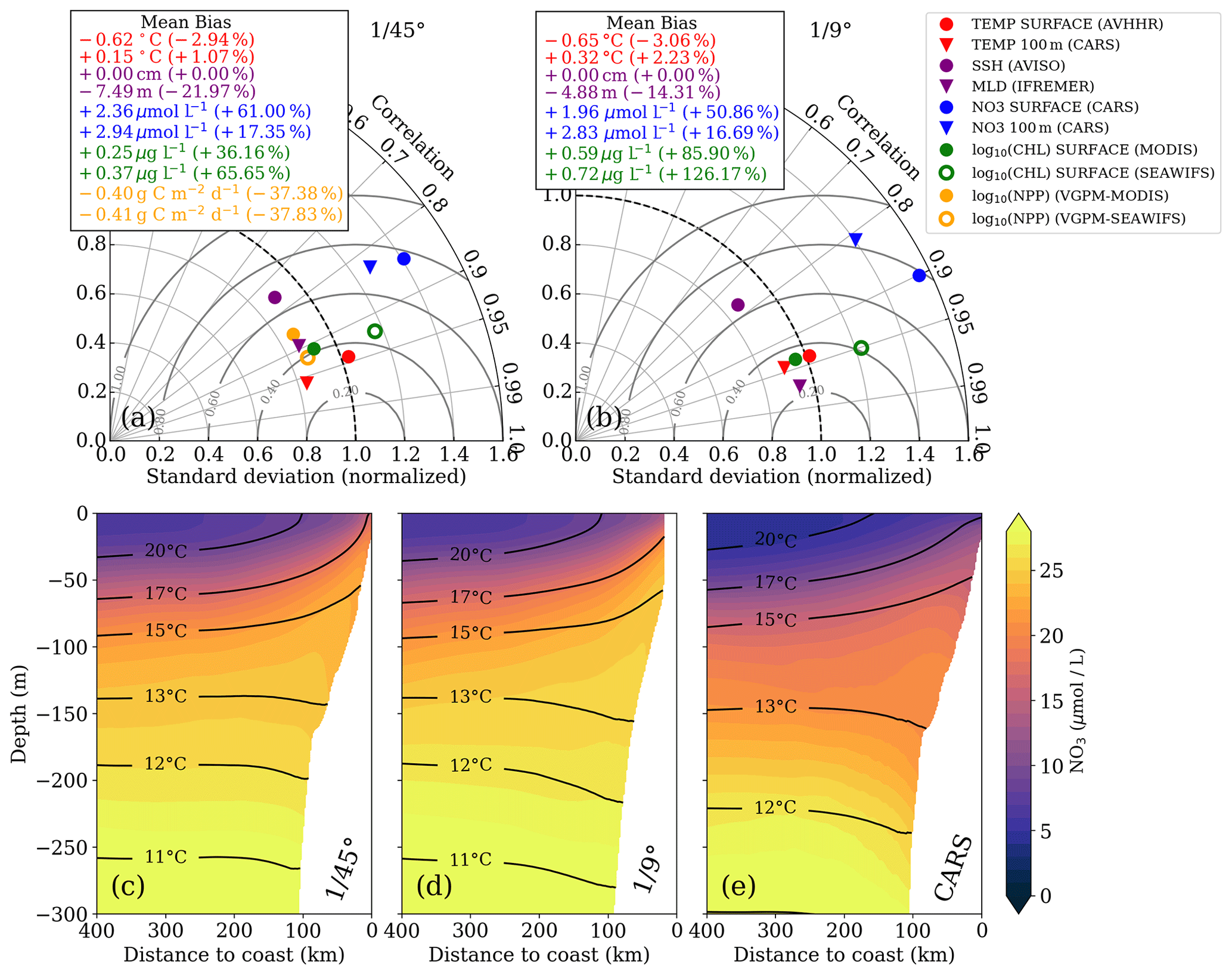
Figure 2Taylor diagrams for (a) ∘ and (b) ∘ simulations, respectively. The statistics were computed from temporally averaged 2-year-mean fields (see Fig. S1) and therefore represent their spatial variability. Due to the strongly skewed distributions of chlorophyll a and PP, these variables were logarithmized prior to computing correlation and standard deviation to approximate normally distributed variables, while the mean bias was calculated using the original values. Gray concentric circles centered around unity-normalized standard deviation and correlation indicate the normalized root mean square error (NRMSE). The analysis for the ∘ simulation was restricted to the extent of the ∘ domain to facilitate direct comparison. Primary-production rates were not saved for the ∘ simulation and could therefore not be evaluated. (c–e) Along-shore-averaged sections of mean nitrate concentrations with temperature contours superimposed for the (c) ∘ simulation, (d) ∘ simulation, and (e) CARS climatology. The CARS climatology was interpolated onto the ∘ model grid before computing the along-shore average.
In this section, we verify that the two simulations realistically reproduce the annual mean physical and biogeochemical structures. The model evaluation focuses here on the horizontal variability over a 2-year averaging period (2015–2016). The comparison of the most relevant physical and biogeochemical variables with observations is summarized in Taylor diagrams for both the ∘ and ∘ simulations (Fig. 2a, b). The corresponding mean horizontal fields are shown in Figs. S1–S6.
The simulated SST shows a negative bias (0.6 ∘C) relative to satellite observations for both simulations. This negative bias is a ubiquitous feature of EBUS simulations (e.g., Dufois et al., 2012) attributed partly to overly strong wind-driven upwelling near the coast (Fig. S1). The spatial patterns of simulated and observed mean SST are highly correlated (r=0.95). This is expected since SST observations are used to calculate the restoring term on the model surface heat flux, thus partly constraining the model SST. At 100 m depth, a weak positive temperature bias is found in both the ∘ simulation (0.32 ∘C) and the ∘ simulation (0.15 ∘C) with respect to CARS. The correlation between the model and observations at this depth is high (r>0.9).
The model mixed layer is slightly shallower (−4.88 m) than the observed IFREMER climatology mixed-layer depth (de Boyer Montégut et al., 2004) in the ∘ simulation, while the MLD bias is slightly larger (−7.49 m) in the ∘ simulation (Fig. 2a, b). The spatial variability in the mean for both simulations is well reproduced (r>0.95), displaying a shallower mixed layer near the coast due to the shoaling of isotherms (Fig. S4). Note that the coarse resolution of the gridded MLD climatology () is a limitation for the MLD evaluation. The SSH bias for both simulations is equal to zero by construction as the time-averaged and spatially averaged sea level has been subtracted from each time series (Fig. 2a, b). Subtracting a reference value has no effect on the pressure gradients which drive the dynamics. The spatial SSH variations are only slightly underestimated in the simulations (10 %), and the spatial correlation between simulated and observed SSH fields is high (r≈0.8; Fig. 2a, b).
The simulated eddy kinetic energy (EKE) calculated from SSH and surface geostrophy is overestimated relative to AVISO satellite observations for both simulations (Fig. S6). The overestimation of EKE amounts to ∼ 37 % for the ∘ simulation and 100 % for the ∘ simulation. There are several possible reasons for this mismatch: firstly, the open boundaries of the relatively small ∘ domain likely do not allow sufficient removal of EKE by westward propagation of eddies. Furthermore, the 2-year averaging period used for this model evaluation is short, and the comparison to observations is difficult due to freely evolving turbulence in the simulations. Lastly, the SSH observations are acquired along satellite tracks, and the mapping of this spatially and temporally uneven data on a uniform grid can introduce biases. For a fair comparison of simulated and observed EKE, the sampling and processing of the satellite data would need to be reproduced with model data. This analysis is beyond the scope of this study, and we can therefore not be certain of the extent to which the EKE in our simulations is overestimated.
We now evaluate the model biogeochemical fields. The model surface chlorophyll is too high in both simulations relative to satellite observations, while the spatial variability in chlorophyll is well reproduced (Fig. 2a,b). The positive bias is reduced in the ∘ simulation by a factor of 2 compared to the ∘ simulation. Despite the positive chl bias, the modeled PP in the ∘ simulation is underestimated with respect to PP estimates derived from ocean color (bias 37 %). Our in situ measurements generally suggest an underestimation of PP in the simulations as well, with the exception of the surface values at the upwelling front (Table 1).
The model tends to overestimate nitrate at surface (bias ∼ +2 µmol L−1) and subsurface (bias ∼ +3 µmol L−1) levels in both simulations (Fig. 2a, b), while the spatial patterns are well reproduced (Fig. S1). In general, nitrate is slightly improved in the ∘ simulation compared to the ∘ simulation. The modeled cross-shore vertical structure of temperature and nitrate is also evaluated using along-shore-averaged mean sections from the two simulations and from the CARS climatology (Figs. 2c–e). Above 100 m depth, the simulated isotherms compare well with the climatology but are slightly steeper within 200 km from the coast and less steep farther offshore, suggesting a slightly too strong coastal upwelling and too weak offshore upwelling by Ekman suction in the simulations. Below 100 m depth, the isotherms slope downward towards the coast, indicative of the Peru–Chile Undercurrent. Nitrate isolines roughly follow isotherms. Modeled nitrate values are too high along the continental slope above 250 m depth. Despite this bias, the horizontal and vertical nitrate gradients above 100 m depth compare well with the CARS climatology (Fig. 2c–e). We can therefore assume that the model realistically represents the nitrate fluxes associated with upwelling and subduction, which occur predominantly in this depth range. Further details on the model evaluation can be found in Hauschildt (2017).
3.1 Physical and biogeochemical upwelling structure in observations and simulations
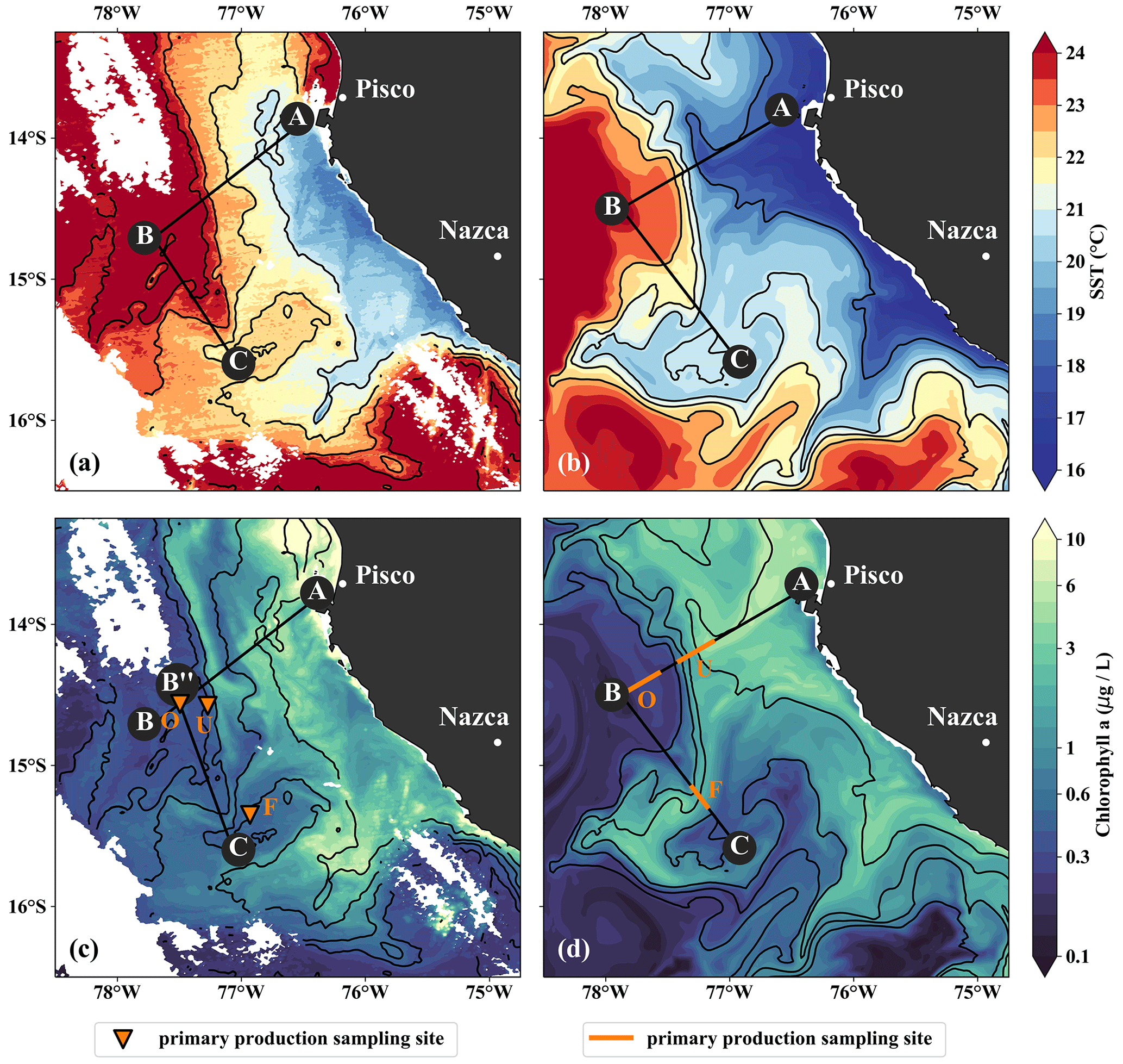
Figure 3(a, b) Sea-surface temperature and (c, d) surface chlorophyll in (a, c) observations on 14 April 2017 and in (b, d) the model simulation on 5 April 2017. Locations of vertical sections are superimposed (see Figs. 4, 5). Orange triangles in (c) indicate three sampling locations – offshore (O), at the upwelling front (U), and in the filament (F) – where primary production was measured. Orange lines in (d) indicate the corresponding locations used for comparison in the simulation. The simulated fields represent 1 d averaged model output.
The filament survey (Sec. 2.1) was carried out during the transition from austral summer to fall during 12–17 April 2017. Being typical for the season, moderate southeasterly along-shore winds between 5–6 m s−1 near the coast and 11–14 m s−1 offshore were observed throughout the survey, which represents upwelling-favorable conditions (not shown). The most intense upwelling is often found in distinct cells near headlands and capes, indicated by along-shore minima of sea-surface temperature (SST). A well-known upwelling cell off Peru can be identified near 15 ∘S by its relatively low SST (18 ∘C) in a satellite image taken on 14 April 2017, 18:25 UTC (Fig. 3a). A strong cross-shore SST gradient exists between this coastal minimum and the warm offshore waters (24.5 ∘C). The maximum SST gradient (0.15 ∘C/km) is found 110–130 km offshore along the 23 ∘ C isotherm and marks the location of the upwelling front. The offshore increase in SST is accompanied by an increase in salinity from 35.3 to 36.25 g kg−1 and an increase in mixed-layer depth from 5 to 30 m, approximately following the σθ = 25 kg m−3 isopycnal (Fig. 4a). Offshore of the upwelling front, a sharp thermocline with vertical temperature gradients of up to 0.4 ∘C m−1 across the base of the mixed layer is found (Fig. 4a). The deepest isopycnal that outcrops at the coast (σθ = 25.5 kg m−3) descends to 50 m depth 75–100 km offshore. The predominant water mass along the density surfaces that supply the coastal upwelling is the Equatorial Subsurface Water (ESSW; e.g., Silva et al., 2009) at a density of about σθ = 26.0 kg m−3 and a salinity of 35.2 g kg−1 (Fig. 4b), which is transported poleward along the shelf by the Peru–Chile Undercurrent (PCUC; Gunther, 1936; Fonseca, 1989; Montes et al., 2010). The maximum poleward velocities of ∼ 0.5 m s−1 are observed within 50 km from the coast at 20–100 m depth (Fig. 4c).
The observed physical variability in the upwelling region gives rise to biogeochemical variability on similar scales (Figs. 3c, 4d, e). Surface chlorophyll concentrations are enhanced inshore of the upwelling front (∼ 5 mg m−3) compared to offshore (∼ 0.3 mg m−3) due to nutrient-rich subsurface waters (15–20 µmol L−1 NO3) that are brought to the surface in the coastal upwelling (Figs. 3c, 4d, e). Surface NO3 concentrations decrease continuously by about 0.1 µmol L−1 per kilometer cross-shore distance to 5 µmol L−1 inshore of the upwelling front (Fig. 4e). Note that a local chlorophyll maximum occurs on the cold side of the upwelling front (∼ 10 mg m−3; Figs. 3c, 4d). Offshore of the upwelling front surface nutrients are depleted (< 1 µmol L−1 NO3), and a strong vertical gradient of up to 2 µmol L−1 NO3 m−1 is present across the base of the mixed layer (Fig. 4e). As a result, the maxima in chlorophyll (7–10 mg m−3; Fig. 4d, Table 1) and PP (∼ 9 µmol C L−1 d−1, Table 1) occur below the mixed layer, where nutrients are abundant (20 µmol L−1 NO3; Fig. 4e). Below 80 m depth chlorophyll concentrations are low (< 0.2 mg m−3) everywhere in the study area (Fig. 4d). Due to low subsurface chlorophyll concentrations in the source waters on the shelf, surface chlorophyll concentrations remain relatively low (∼ 1 mg m−3) within 20–30 km from the upwelling center and only peak (4–6 mg m−3) farther offshore (Figs. 3c, 4d). This illustrates that despite the clear inverse relationship of chlorophyll and SST on larger scales, small-scale chlorophyll variability is more complex and not consistently related to SST.
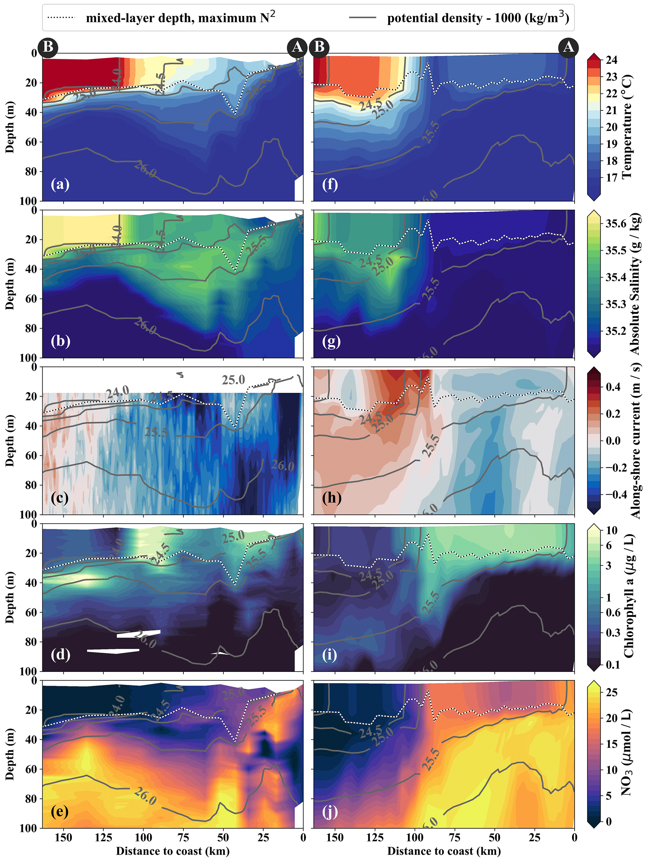
Figure 4Cross-shore sections of (a, f) temperature, (b, g) salinity, (c, h) along-shore current, (d, i) chlorophyll, and (e, j) nitrate in observations (a–e) and model simulations (f–j). Potential-density contours are shown in gray, and mixed-layer depth is represented by the broken white–black line. Letters A and B indicate the section endpoints marked in Fig. 3. The model sections represent 1 d averaged output on 14 April 2017.
From the model simulation, we chose one particular event that reproduces physical conditions similar to those of the survey and assessed the ability of the model to capture the dynamics observed in situ. The characteristic structure of coastal upwelling in the physical fields for this particular event is well reproduced in our simulations, but some differences exist (Figs. 4a–c, f–h). The location of the upwelling front 100 km offshore and the corresponding Δ SST maximum of 0.2 ∘C km−1 agrees well with both satellite images and in situ measurements (Figs. 3a, b, 4a, f). The temperature and salinity distributions are, overall, similar to observations in the simulation, apart from a cold and fresh bias of the surface waters inshore of the upwelling front (Figs. 4a, b, f, g). Due to this bias the σθ = 25 kg m−3 isopycnal outcrops 100 km offshore in the simulation and near the coast in the observations. The average mixed-layer depth in the simulation is ∼ 20 m, very close to observed values offshore of ∼ 100 km. However, the observed mixed-layer depth decreases to only ∼ 5 m in the coastal upwelling patch, whereas such a shallow mixed layer is not seen in the simulation (Fig. 4a, f). The southward velocities of ∼ 0.3 m s−1 inshore of the upwelling front in the simulation that are associated with the surfacing undercurrent are similar to observations (Fig. 4c, h). However, the strongest southward flow (∼ 0.3 m s−1) in the simulation is weaker than observed (∼ 0.5 m s−1) and not located at the shelf but 55 km offshore. This is likely related to differences in mesoscale variability since an anticyclone is present immediately offshore of the upwelling patch in the simulation compared to a cyclonic eddy at approximately the same position in the observations (not shown). Averaging over the period 2015–2016 yields an alongshore velocity of 13 cm s−1 in the core of the PCUC, which is close to the observed velocity (∼ 14 cm s−1; Chaigneau et al., 2013).
In the simulation, the upwelling structure also dominates the variability in the biogeochemical fields (Figs. 3d, 4i, j). Chlorophyll concentrations above 0.2 mg m−3 are found down to 80 m (100 m) in the observations (simulation), showing overall good agreement (Fig. 4d, i). Maximum surface chlorophyll values in the observations (> 10 mg m−3) and in the simulation (∼ 8 mg m−3) are also reasonably similar. However, the cross-shore and vertical gradients of surface chlorophyll reveal notable differences between the observations and the simulation: local maxima of up to 10 mg m−3 are present along the nutricline and at the upwelling front located more than 100 km offshore in the observations, while chlorophyll concentrations in the simulation show no such maxima, are inversely related to SST, and decrease almost continuously offshore and with depth (Fig. 3, 4d, i). Lastly, it is a common feature in satellite images of chlorophyll that concentrations remain relatively low (< 1 mg m−3) in recently upwelled waters near the coast (30 km) and only increase to > 3 mg m−3 farther offshore (Fig. 3c). This behavior is to some degree reproduced in the simulation but only within a much narrower (∼ 10 km) region along the coast (Fig. 3d). The observed nutricline – here defined as the 10 µmol L−1 nitrate contour – is located between 20 and 50 m depth in the open ocean and intersects the surface near the coast where upwelling occurs (Fig. 4e). The modeled nutricline locally reaches depths of 100 m in the open ocean and also reaches the surface near the coast (Fig. 4j). Surface nitrate maxima of 5 µmol L−1 associated with filaments in the simulation are comparable to the observations.
In brief, the observed near-surface cross-shore gradients of temperature, nitrate, and chlorophyll are well represented in the simulations. In the following section we see how both observed and modeled cold filaments give rise to along-shore variability by advection across these gradients.
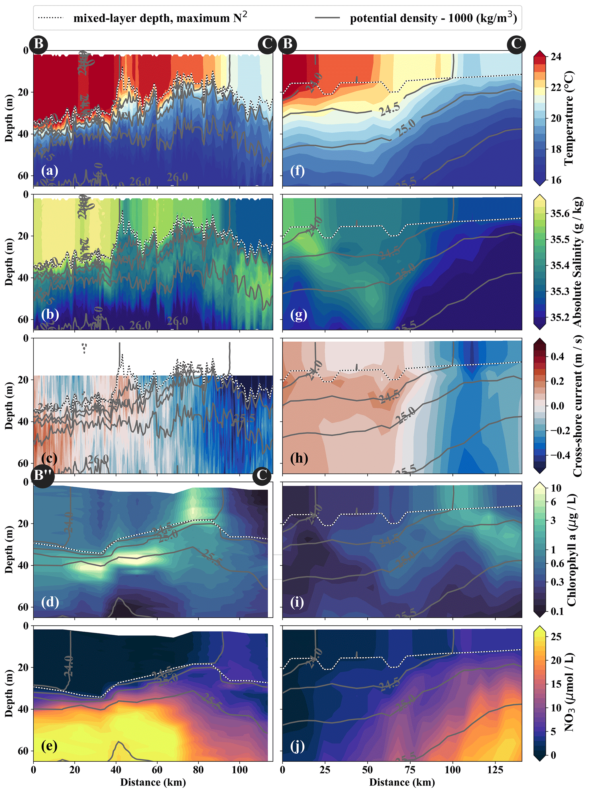
Figure 5Same variables as in Fig. 4. Note the slightly different endpoints of the physical and biogeochemical section in the observations (see B and B” in Fig. 3). The model sections represent 1 d averaged model output on 14 April 2017, which was chosen for the horizontal and vertical gradients to be as sharp as possible and directly comparable to observations.
3.2 Physical and biogeochemical characterization of observed and modeled filaments
In the observations, cold filaments dominate the along-shore variability in physical and biogeochemical parameters near the surface (Figs. 3a, c, 5a–e). Two cold filaments with temperatures of 21.5 and 20.5 ∘C in their respective centers extend offshore from the upwelling center, separated by a ∼ 30 km wide intrusion of 1 ∘C warmer water (Fig. 3a). Their along-shore position matches with two SST minima (19 ∘C) at the coast, suggesting that they carry recently upwelled water. In the following we focus on the relatively narrow (10–20 km) northern filament at 15.25∘ S, 77∘ W because of multiple available physical and biogeochemical measurements. The filament can be identified in satellite SST images already on 22 March. It changed its position only by 𝒪(10) km until it was sampled on 15 April (not shown). The associated SST fronts are present the entire time but vary in strength and position. The physical structure of the filament and the distribution of the biogeochemical parameters are characterized in the following.
The cold filament is associated with along-shore variability in the physical and biogeochemical fields in the mixed layer (Fig. 5a–e). It is characterized by a pronounced minimum in temperature (20 ∘C) and salinity (35.2 g kg−1) in the mixed layer at the southern end (110 km) of transect PHY (Fig. 5a, c). The minimum temperature found in the filament on transect PHY is at least 1.5 ∘C colder than suggested by the satellite SST (Figs. 3a, 5a). This mismatch is likely related to the diurnal cycle of solar insolation and differential heating as PHY crossed the filament in the early morning, but the SST image was recorded the day before shortly after noon. The low salinity is characteristic of ESSW along the shelf (see Sect. 3.1) and thus indicates that the filament contains recently upwelled water, which is transported to the open ocean by an offshore flow of up to 0.5 m s−1 within the mixed layer (Figs. 5c). The subsurface flow is mainly offshore at the southern end of transect PHY as opposed to onshore flow at its northern end, which is related to a cyclonic mesoscale eddy (not shown). Weak stratification below the filament between the 24.5 and 25 kg m−3 isopycnals (not shown) points to water that has been in the mixed layer recently and could indicate subduction by submesoscale frontal processes. Low-salinity anomalies (35.3 g kg−1) in the same density range below the filament support this hypothesis (Fig. 5b).
Along with the physical properties, the filament creates along-shore variability in the biogeochemical parameters (nitrate, chlorophyll) by advecting recently upwelled water offshore into the open ocean (Fig. 5d, e). Nutrient concentrations in the mixed layer are enhanced in the filament (4–7 µmol L−1 NO3) compared to the surrounding waters (< 1 µmol L−1 NO3), while the highest nitrate concentrations are found near the filament's northern edge (Fig. 5e). A local NO3 maximum is located at the base of the mixed layer (Fig. 5e). Despite elevated nutrient concentrations, chlorophyll concentrations are very low (< 0.1 mg m−3) within the filament, comparable to those found below the euphotic zone (Fig. 5d). PP in the filament is still relatively high, with a maximum (7.5 µmol C L−1 d−1) at 10 m depth within a 35 m deep mixed layer (Table 1). High chlorophyll concentrations (∼ 8 mg m−3) are only found at the northern edge of the filament 75 km along transect BIO (Fig. 5d). Outside the filament, surface waters are nutrient-depleted (< 0.2 µmol L−1), while high nutrient concentrations (25 µmol L−1 NO3) are present just below the mixed layer (Fig. 4e). The maxima in chlorophyll (> 10 mg m−3) and PP (9.4 µmol C L−1 d−1; Table 1) are therefore located below the mixed layer (∼ 40 m), where nutrients are abundant (Fig. 5d, e; Table 1). Below 80 m depth, chlorophyll concentrations are low everywhere along the transect (< 0.1 mg m−3), and primary production is low (< 0.1 µmol C L−1 d−1) at the upwelling front, offshore, and in the filament (Figs. 3c, 4d; Table 1). Notably, surface PP is a factor of 2 higher in the filament than at the upwelling front (3.6 µmol C L−1 d−1), while the latter dominates the offshore chlorophyll variability in satellite images, with surface chlorophyll concentrations about a factor of 4 higher than in the filament (Fig. 3c).
The position and shape of simulated filaments are determined largely by the mesoscale eddy field, which evolves freely in the simulation and can therefore not be expected to correspond to the variability in the real ocean at any given time. The occurrence of major upwelling events and their effect on the variability in fronts and filaments, however, are closely related to the wind forcing of the model, which was derived from satellite-based, daily ASCAT scatterometer winds. We therefore picked simulated filaments that were as close as possible in space and time to the observations, which were then taken as representative of the area and season when the observations were carried out. The chosen filaments are comparable in scale to the observed cold filament, which had an offshore extent of 150–200 km (Fig. 3a, b). Similar to satellite images, the simulated surface fields of SST and chlorophyll show two separate filament structures originating in the upwelling patches off Pisco and Nazca on 5 April 2017 (Fig. 3b, d). For comparability, we focus here on the northern filament, whose location near the upwelling front is similar to the one observed. The modeled filament is associated with pronounced along-shore variability in the physical and biogeochemical fields (Fig. 5f–j). Offshore velocities are present in the filament down to 100 m depth, with a maximum located in the mixed layer (0.4 m s−1; Fig. 5h). Surface minima of temperature (20 ∘C) and salinity (35.25 g kg−1) and maxima of chlorophyll and nitrate are associated with the filament (Fig. 5f–j). Enhanced nitrate concentrations of 5 µmol L−1 are present in the filament, and a shallowing of the nutricline is found in the same location, associated with doming isopycnals between σθ = 25 kg m−3 and σθ = 25.5 kg m−3 (Fig. 5j). Elevated chlorophyll concentrations of 2 mg m−3 are found at its northern edge, marked by the σθ = 24.5 kg m−3 isopycnal outcrop (Fig. 5i). PP in the modeled filament is enhanced relative to the surrounding offshore waters, similarly to observations (Table 1). However, the modeled PP is only enhanced where high chlorophyll concentrations are found, which is not the case for the observations where high PP inside the filament coincides with low chlorophyll. Vertical gradients of PP are also different in the model compared with observations: while there is a strong chlorophyll maximum below the mixed layer that is associated with higher PP than at the surface, subsurface maxima of chlorophyll are rare and weak in the simulation, and PP generally decreases with depth. Despite these differences, the modeled mixed-layer PP has a realistic order of magnitude offshore, at the upwelling front, and in the filament (Table 1).
Table 1Observed and modeled primary production for different dynamical regimes, each at three different depths. The first sample was always taken at 10 m, while the remaining two were placed in the chlorophyll maximum below the mixed layer (25–40 m, ∼ 10 % surface PAR) and a chlorophyll minimum below the euphotic zone (70–80 m, ∼ 1 % surface PAR). Sampling sites and the corresponding model locations used for comparison are marked with letters O, U, and F in Fig. 3c, d. Standard deviation represents triplicate samples for the PP observations, ±3 m bottle depth for the corresponding chlorophyll fluorescence profiles, and differences between individual grid points for the model data.

In summary, the simulation exhibits upwelling filaments that are similar to those observed in aspects like lateral and horizontal scale and offshore extent. Our direct rate measurements indicate that PP in the modeled filaments is comparable to observations. Despite very low chlorophyll concentrations (< 0.1 mg m−3) in the observed filament, surface PP is higher than at the upwelling front by a factor of 2. This highlights the benefits of measuring PP in addition to chlorophyll for model validation to ensure a realistic representation of the underlying processes.
3.3 Timescales of nutrient transport and uptake in observations and models
To analyze the physical and biogeochemical processes in the upwelling system in more detail and over a larger area, we released virtual floats in our submesoscale-permitting simulation. By tracking biogeochemical variables along float trajectories, we studied the biological response to upwelling and subduction in a reference frame following the upwelled water. The upwelled floats originate at depths between 20 and 120 m, the maximum depth agreeing well with the maximum depth of outcropping isopycnals (Figs. 4, 6a). Using the physical and biogeochemical properties averaged over all floats after grouping into subducted and not-subducted ones, we can diagnose the biological response to upwelling and the corresponding timescale (Fig. 6a–e). Phytoplankton growth in PISCES increases exponentially with photosynthetically available radiation (PAR) and also increases as a function of temperature (Sect. 2.5, Eq. 5). PP and chlorophyll along the float trajectories thus increase exponentially a few days before upwelling as the floats move to shallower depths, where both PAR and temperature are higher, and phytoplankton biomass accumulates (Fig. 6a–c). For the floats that are not subducted and remain within the euphotic zone, chlorophyll peaks 15.3 d after upwelling (4.1 mg m−3), followed by a peak in PP after 17.1 d (13.1 µmol C L−1 d−1). For the subducted floats these timescales are slightly shorter: chlorophyll peaks after 14.5 d (2.0 mg m−3), and PP peaks after 13.4 d (4.0 µmol C L−1 d−1).
The fate of upwelled floats is closely related to their change in temperature after upwelling; thus the correct representation of the temperature gradient in the model is crucial (Fig. 3a, b). Water that is warmed rapidly by surface heat fluxes or mixed with warmer offshore waters remains at shallower depths, where sufficient light allows for PP and nutrient uptake. In contrast, floats with little temperature change after upwelling are more quickly removed from the euphotic zone by subduction. Average PP of the subducted floats reduces to 0.1 µmol C L−1 d−1 after 20 d because they are all located below the euphotic zone at this time (Fig. 6b). In contrast, average PP of the floats that are not subducted is still at 6.4 µmol C L−1 d−1 after 20 d.
Nitrate concentrations of subducted floats decline to 16.5, which is 1.5 µmol L−1 lower than upwelled concentrations (Fig. 6e). These numbers show that along the subducted trajectories only a small fraction of the upwelled nitrate is taken up by phytoplankton. In contrast, along the trajectories of those floats that remain in the euphotic zone, phytoplankton can utilize more nitrate. This is indicated by nitrate concentrations of 12.0 µmol L−1 20 d after upwelling, which is 7.1 µmol L−1 lower than upwelled concentrations. Using the subduction ratio (Eq. 7) defined in Sect. 2.5, we estimate that 20 d after being upwelled 40.6 % of the upwelled nitrate is subducted (Fig. 6f). More detailed statistics of the float experiment are given in Table 2. Nitrate concentrations in the observed filament around 150 km offshore reach only 20 %–50 % of those measured near the coast and decrease continuously with offshore distance on cross-shore transect CROSS (Fig. 3e). This suggests that upwelled nitrate fuels a substantial amount of the observed PP. To estimate a timescale over which the observed nitrate uptake occurs, we use offshore velocities of 0.3–0.5 m s−1 found in the filament. These velocities yield an advection time of 3.5–5.8 d from the upwelling center to reach the filament 150 km offshore. This timescale represents a lower bound since the actual path that the water parcel took is unknown and likely longer than a straight line. Initial nitrate concentrations of 15 µmol L−1 in the upwelled water and 5 µmol L−1 in the filament yield a nitrate reduction of 10 µmol L−1 over this time period, which is well within the uncertainty in the modeled estimate.
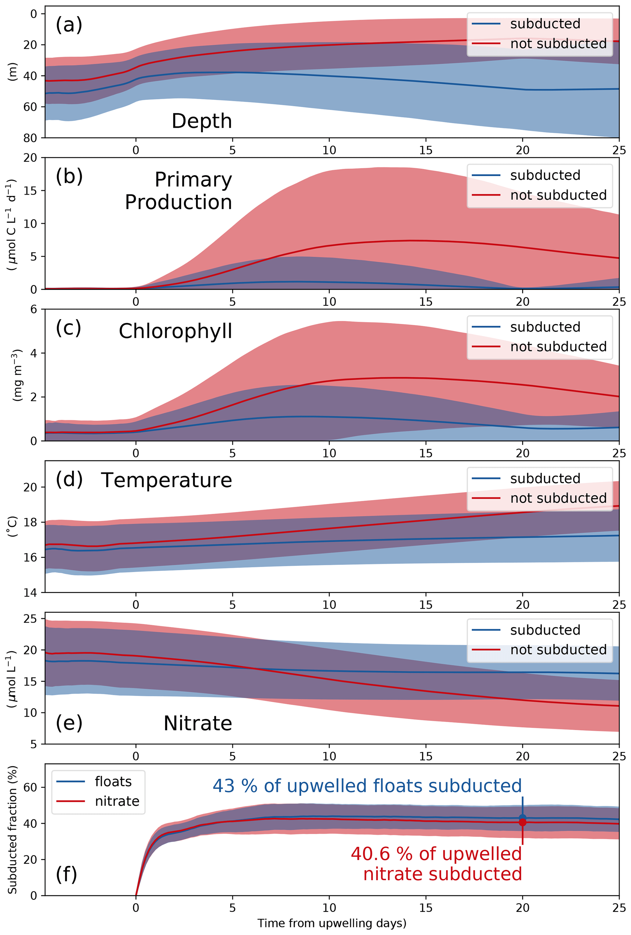
Figure 6(a) Depth, (b) primary production, (c) chlorophyll, (d) temperature, and (e) nitrate averaged over all subducted (solid) and not-subducted (dashed) floats from 20 ensemble members. Blue and red shading indicates the range of ±1 standard deviation based on all subducted and not-subducted floats, respectively. (f) Subducted fraction of floats and nitrate. Shaded areas represent the range of ±1 standard deviation based on 20 ensemble members. The results shown here are based on the submesoscale-permitting (∘) simulation.
3.4 Effect of resolution on the biogeochemistry of the Peruvian upwelling
With the purpose of quantifying the impact of the different dynamics at submesoscale-permitting ( ∘) resolution on upwelling and subduction of nutrients, we repeated the above float experiment using the mesoscale ( ∘) model flow field and compared both results (Table 2). In the mesoscale experiment, the mean nitrate concentration of upwelled floats is 2.4 µmol L−1 higher than in the submesoscale experiment. For the subducted floats, this higher initial nitrate concentration is overcompensated by a higher uptake along the float trajectories so that offshore nitrate concentrations are 2 µmol L−1 lower in the mesoscale simulation. For the floats that were not subducted, increased nitrate uptake in the mesoscale simulation also overcompensates the initially higher concentrations so that offshore nitrate concentrations are 5 µmol L−1 lower in the ∘ compared to the ∘ simulation. This higher nitrate uptake for both subducted and not-subducted floats in the ∘ simulation can be explained by on average shallower float trajectories (Fig. 7) and therefore higher light levels and higher PP compared to the ∘ simulation. Accordingly, subduction of upwelled nitrate is reduced by 13.9 % in the ∘ simulation compared to the ∘ simulation, while the maxima of PP and chlorophyll along the averaged trajectories are increased by 5.3 µmol C L−1 d−1 and 2.2 mg m−3, respectively (Table 2).
Table 2Diagnosed variables from the virtual float ensembles in the ∘ and ∘ simulations. “Peak” values represent the maximum of the average over floats of one simulation.
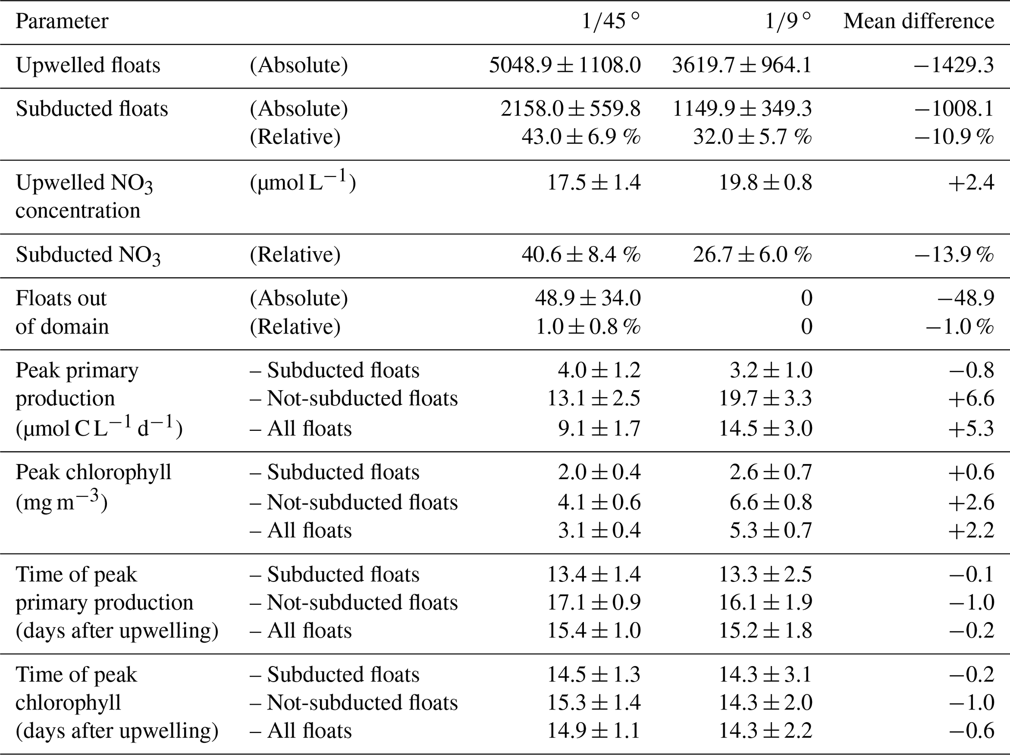
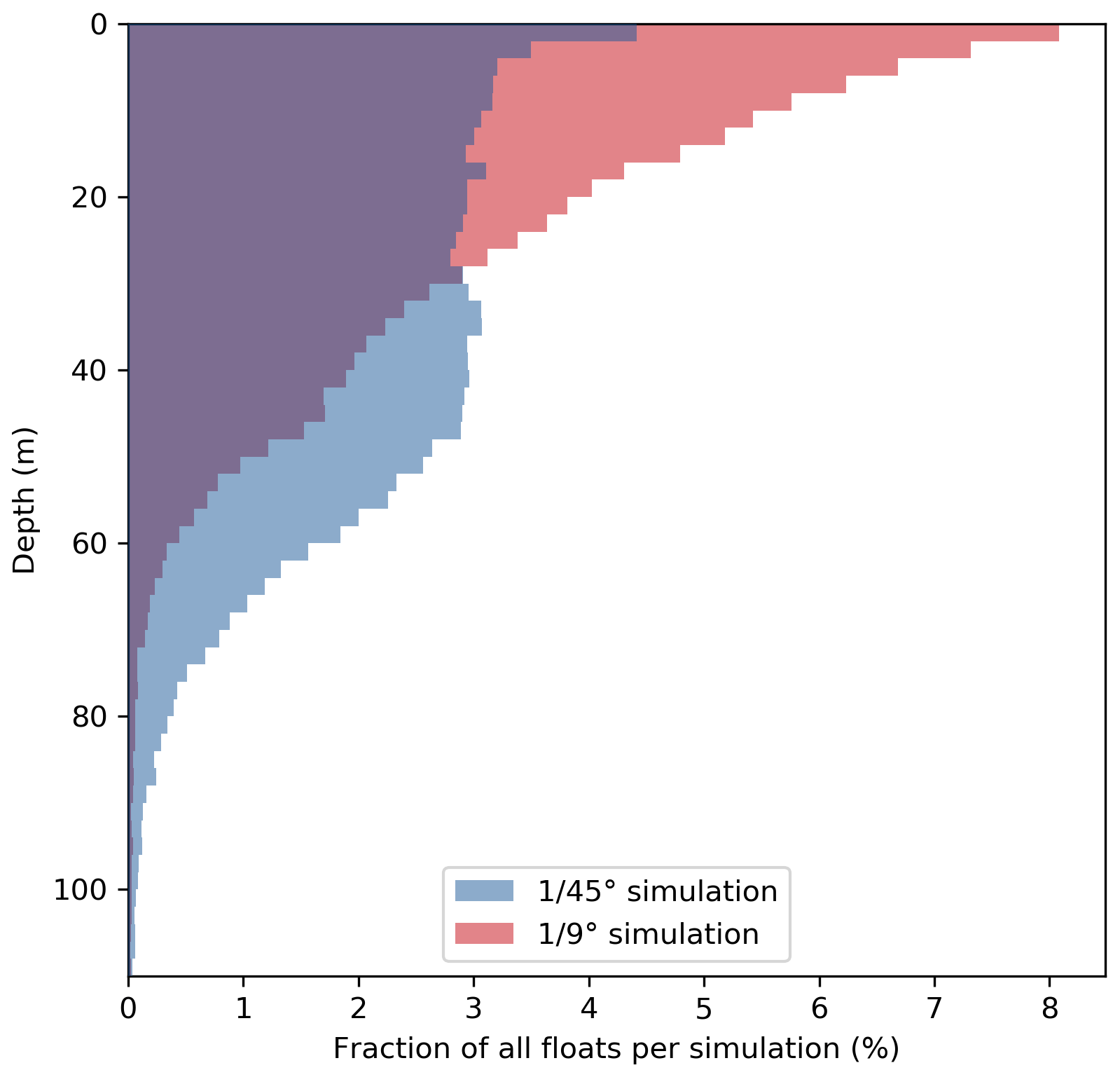
Figure 7Vertical distribution of all upwelled floats from the float experiment ensemble 20 d after upwelling in the and ∘ simulations. Histograms were generated using 2 m vertical bins.
This increased subduction in the ∘ simulation is also apparent in the vertical float distribution 20 d after upwelling (Fig. 7). The vertical maximum of the float distribution is located in the top 5 m for the both simulations, but below this surface peak the distributions are very different: in the ∘ simulation the majority of floats are evenly distributed between 5–50 m depth, while in the ∘ simulation the float abundance sharply decreases downward from a much more pronounced surface peak. The maximum depth reached by float trajectories is deeper by about 30 m in the ∘ simulation (Fig. 7). Comparing the same virtual float experiment in different model configurations nicely illustrates the relative changes in subduction and their biogeochemical impacts. However, note that this Lagrangian approach is restricted to short integrations during one season and is less suited to obtain estimates of absolute changes in the time-averaged model fields.
The impact of increased horizontal resolution on the long-term-averaged biogeochemical fields can be approximated based on the difference between the coarse- ( ∘) and high-resolution ( ∘) simulations. In a first-order assessment, this difference can be taken to represent the influence of submesoscale frontal processes and the associated horizontal and vertical eddy fluxes that are additionally resolved in the high-resolution simulations, an assumption that is justified by the pronounced increase in eddy kinetic energy by a factor of 2 from coarse to high resolution (Fig. 8a). The changes in nitrate due to the effect of submesoscale-permitting resolution in the simulations are greatest within 25 km from the coast in the upper 200 m of the water column, where a pronounced decrease in nitrate (−2.5 µmol L−1; Fig. 8b) is apparent. These reduced subsurface nitrate concentrations in the ∘ simulation compared to the ∘ simulation are consistent with ∼ 2 µmol L−1 lower nitrate concentrations of upwelled floats (Table 2). In a tongue that extends from this minimum ∼ 250 km offshore along the nutricline, a smaller decrease in nitrate (∼ −1.5 µmol L−1; Fig. 8b) is seen. Offshore of this negative change, an increase in nitrate (∼ 1.5 µmol L−1) is apparent at around 100 m depth when switching from ∘ to ∘ resolution. The offshore nitrate increase together with increased eddy kinetic energy (EKE) in the ∘ simulation suggests that an increase in the cross-shore nitrate flux takes over once the nitrate is removed from the surface (Fig. 8a, b). Horizontally, the regions of large nitrate differences when switching from to ∘ resolution coincide with regions of increased eddy kinetic energy at ∘ resolution (not shown). Near the coast and at a depth of 300 m to 500 m, nitrate increases (∼ 2 µmol L−1) when switching from ∘ resolution to ∘ resolution, directly below the strong nitrate decrease in the top 200 m (∼ −2.75 µmol L−1). A plausible explanation for this pattern is that due to increased offshore transport in the submesoscale simulation, sinking organic matter can reach greater water depths that are disconnected from the upwelling. Accordingly, this would mean that there is less accumulation and remineralization of organic matter on shallow shelf areas. This decrease in local remineralization on the shelf would then result in a downward redistribution of nitrate similar to the “nutrient leakage” described in Gruber et al. (2011). However, small differences in the alongshore mean circulation along the continental slope (not shown) may also modify the nitrate content of the water masses. Disentangling these processes is beyond the scope of the present work. A decrease in chlorophyll of 1 mg m−3 near the coast and 0.3 mg m−3 300 km offshore between the and ∘ simulations is seen at the surface (Fig. 8d). This decrease in surface chlorophyll coincides with an increase in surface nitrate (+0.5 µmol L−1), pointing to reduced nitrate uptake due to limitation of phytoplankton growth by nutrients other than nitrogen. In order to understand the reason for this model behavior, we diagnosed which nutrient is limiting primary production in the simulation for the surface layer at every grid point and time step. We identified a decrease in surface iron concentrations by 50 % in the ∘ simulation (Fig. 8c), leading to a shift from nitrogen to predominantly iron limitation in a 50 km wide band close to the coast over most of the year (not shown). Given that the coastal area is where most production occurs, increased subduction of upwelled iron in addition to nitrate subduction in the ∘ simulation could contribute to the reduced productivity at the surface.
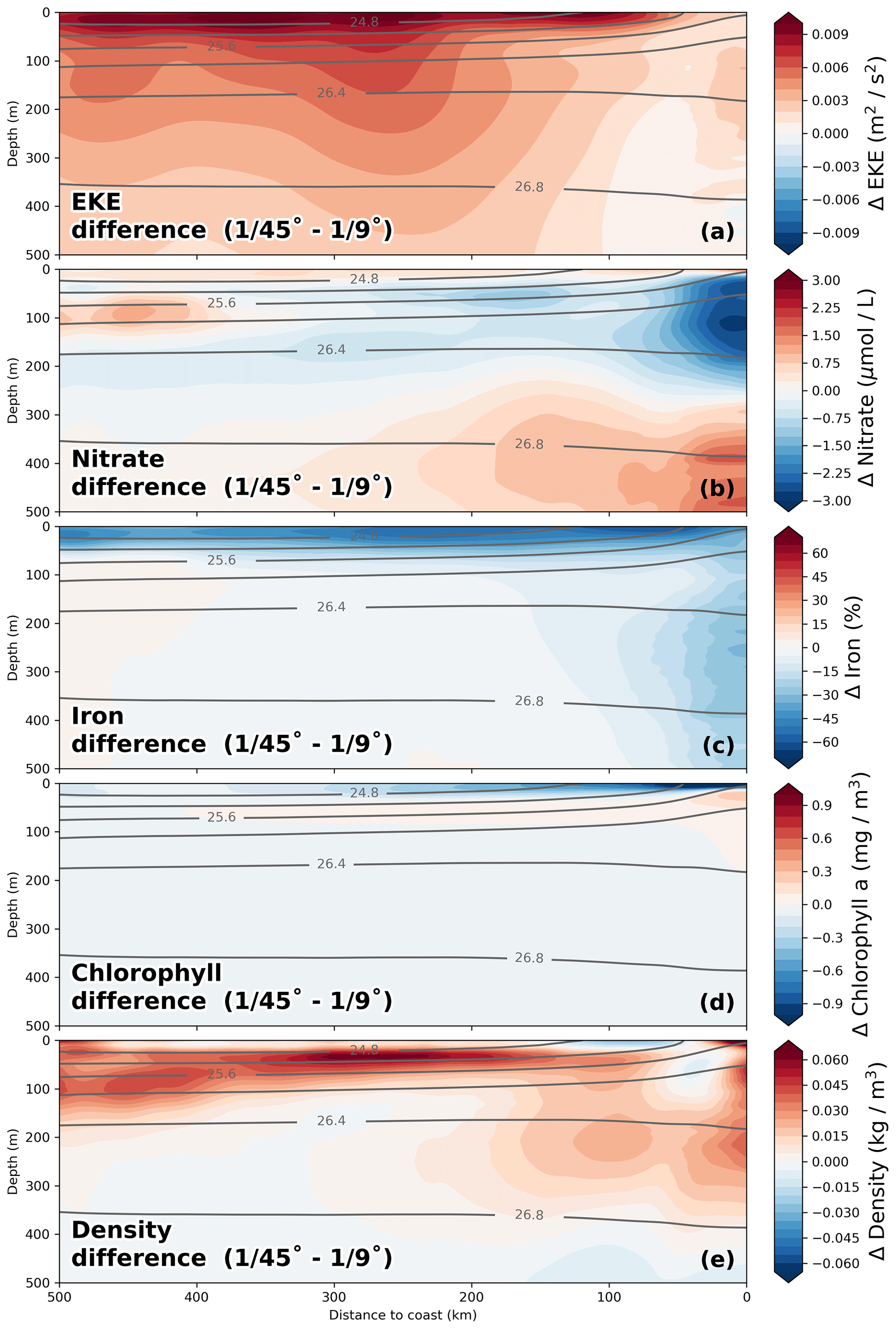
Figure 8Relative differences in (a) nitrate, (b) iron, (c) chlorophyll, (d) temperature, and (e) eddy kinetic energy (EKE) between the and ∘ simulations calculated as –. EKE was calculated relative to a 6-month running mean. All fields were averaged on depth levels in the along-shore direction with 25 km cross-shore bins in a coastal band of 500 km width between 10.5 and 17.5 ∘S over the period 2015–2016. Gray lines represent potential density averaged over the and ∘ simulations.
Using an integrated approach of in situ observations and modeling, we estimated that 40 % of the upwelled nitrate off Peru is subducted without being utilized by phytoplankton. While the agreement between observed and modeled synoptic variability introduced by filaments and fronts lends some confidence to our results, there are uncertainties and limitations which are discussed in the following.
4.1 Primary production
The range of PP rates that were determined experimentally from incubations (Table 1) are very close to measurements by Dengler (1985) acquired during April–June 1976 in the upwelling center near 15∘ S (4–16 µmol C L−1 d−1), increasing confidence in our results. In October 2005, Fernández et al. (2009) observed a similar range of PP rates in the top 25 m of the water column slightly north (3–16.5 µmol C L−1 d−1; 11–12∘ S) and south (1–3.5 µmol C L−1 d−1; 16–18∘ S) of our study area. The PP rates diagnosed from the biogeochemical model simulations are close to our observed PP rates. Moreover, they represent the horizontal variability between different dynamical regimes in the study region relatively well (Table 1), except for the offshore waters, where the modeled subsurface PP is likely too low. Satellite-based estimates of mean NPP suggest that the vertically integrated PP in the model is biased low (∼ −37%; Fig. 2a).
Our PP observations within the filament do not distinguish between regenerated production from ammonium and new production from nitrate (Dugdale and Goering, 1967). Regenerated nitrogen can locally account for as much as 50 % of surface primary production off southern Peru (Fernández et al., 2009). However, nitrate concentrations measured in the filament 150 km offshore are only 20 %–50 % of those measured near the coast, and nitrate appears to decrease with offshore distance on transect CROSS (Fig. 4). This is an indicator that a substantial amount of PP in the region of the filament survey near 15∘ S is fueled by newly upwelled nitrate. Using observed velocities we estimated that a reduction in nitrate concentrations by 10 µmol L−1 occurs over the course of 3.5–5.8 d while the water is advected offshore. Assuming this reduction in nitrate concentrations occurs only due to phytoplankton growth in a closed volume would require PP rates of 11.4–18.9 µmol C L−1 d−1 (using a C : N ratio of 6.625 after Redfield, 1963). This estimate is higher than the ∼ 7.5 µmol C L−1 d−1 measured in the filament, possibly pointing to nitrate being removed from the surface waters due to subduction and diffusion processes. Admittedly, large uncertainties are associated with this crude estimate since it is likely that (1) PP in the upwelled water did not remain constant, (2) the ratio of C and N uptake did not correspond exactly to the Redfield ratio, (3) the water parcel did not travel offshore in a straight line, (4) it was subject to mixing with the surrounding water, and (5) local remineralization of nutrients took place. Nevertheless, it provides a useful illustration that advected nitrate from the upwelling patch near the coast is more than sufficient to support the observed phytoplankton growth inside the filament. It is therefore reasonable to assume that a substantial fraction of PP occurring within the filament is fueled by newly upwelled nitrate. Similar to the observed filament, the simulated filaments still contain ∼ 5 µmol L−1 of nitrate ∼ 150 km offshore, suggesting that the nitrate uptake in the simulations is realistic.
Along-shore variability in PP in the simulation is closely related to chlorophyll concentrations, while the observed relationship of PP and chlorophyll is less clear (Table 1). Investigating the reasons for this discrepancy is beyond the scope of this study and left for future work, but we can speculate that it is related to the relatively simple parameterization of primary production in PISCES (see Sect. 2.5). For example, changes in the phytoplankton physiology or species composition of the phytoplankton community are not modeled. These would likely allow stronger variations in the chlorophyll-to-carbon ratio of phytoplankton (Sect. 2.5, Eq. 5). Another missing process is the aging or health of the phytoplankton population, which could slow down PP, while chlorophyll concentrations remain high, and thereby decouple the two parameters. Note that a new version, PISCES-quota (Kwiatkowski et al., 2018), will be able to represent more elaborate phytoplankton stages in future studies. The modeled PP strictly decreases with depth corresponding to decreasing light levels, while in the observations subsurface maxima of PP are found offshore and at the upwelling front (Table 1). The subsurface chlorophyll maximum is too weak and diffuse in the simulations, which is consistent with this difference in the vertical distribution of PP. This could be partly related to dynamical bias in the simulations: near-surface stratification at the base of the mixed layer is lower in the model than in the observations by a factor of 2–3, which likely results in a too diffuse offshore nutricline and contributes to the weak subsurface chlorophyll maximum. For the reasons mentioned above, subsurface PP in the offshore waters is likely too low in our simulations.
4.2 Impact of the mean nitrate bias on subduction estimates
We use the fraction of all upwelled floats that have been subducted 20 d after upwelling for quantifying changes in the associated nutrient fluxes. These float trajectories represent only advective pathways, but the tracer concentrations along the trajectories include the effects of diffusion and surface mixing. At submesoscale-permitting resolution and for short integration times it is reasonable to assume that advection is dominant. A mean bias of nitrate in the ∘ simulation (see Sect. 2.8) could have an effect on the results of our Lagrangian analysis. We identified a positive nitrate bias of ∼ 61% at the surface and ∼ 17 % at 100 m depth relative to the CARS climatology (Fig. 2a). A positive nitrate bias of similar magnitude (6–8 µmol L−1) has also been documented by Espinoza-Morriberon et al. (2017) in their regional PISCES simulations off Peru. The positive nitrate bias suggests an overestimation of the upwelling fluxes of nitrate. Since the nitrate concentrations in the coastal upwelling region are generally high, the limiting effect of nitrate on PP in this region is small. The nitrate bias is therefore unlikely to have a substantial effect on the nitrate uptake due to PP that occurs before subduction.
The nitrate bias, however, can still impact our estimate of the subducted nitrate fraction (Eq. 7, Fig. 6f). To obtain a first-order estimate of the uncertainty due to this bias, we compute the subduction ratio again from averaged mean quantities along the float trajectories. In this case Eq. (7) can be simplified to
where F is the respective number of upwelled and subducted floats, and angled brackets denote averages over all subducted float trajectories. The subducted float fraction is 0.43 in our study, corresponding to 43 % of all upwelled floats being subducted. The second term in the parentheses is the ratio between the nitrate uptake after upwelling, ΔNO3, and the sum of upwelled nitrate concentration NO and nitrate bias . Because the nitrate bias occurs in the denominator, it leads to an overestimation of the subducted nitrate fraction. To approximate this error, we insert averaged values from our float experiments (Fig. 6e) into Eq. (8): for the ensemble mean values of our float experiment (ΔNO3 = 1.5 µmol L−1, NO + µmol L−1) we obtain a subducted nitrate fraction of 39 %, close to our original estimate (40.6 %; Fig. 6f). Correcting for an assumed positive nitrate bias of 6.5 µmol L−1 (Fig. 2c, e; ΔNO3 = 1.5 µmol L−1, NO = 10 µmol L−1), we obtain a subducted float fraction of 36.5 %. Note that this calculation so far assumes that ΔNO3 is unbiased. We can instead assume that ΔNO3 exhibits a negative bias of −0.9 µmol L−1 proportional to the negative PP bias (−37 %). Correcting for this bias (ΔNO3 = 2.4 µmol L−1, NO = 10 µmol L−1) yields a subducted nitrate fraction of 30.5 %, which can be viewed as a lower estimate.
In summary, we conclude that the mean biases of nitrate and PP in the ∘ simulation likely result in an overestimation of the subducted nitrate fraction, with a lower bound of 30.5 % of upwelled nitrate being subducted.
4.3 Nitrate subduction
We estimated the impact of submesoscale frontal processes by comparing virtual float experiments in the and ∘ simulations and found that subduction of nitrate is 13.9 % higher at submesoscale-permitting resolution. A decrease in mean PP by about one-third when switching from to ∘ resolution is also seen along float trajectories (Table 2). The difference between 2-year-averaged fields also shows subsurface nitrate concentrations being lower by about 2.5 µmol L−1 within 200 km from the coast in the ∘ simulation (Fig. 8b), further supporting this interpretation. These results suggest that submesoscale frontal processes amplify the mesoscale effects found in previous studies (Gruber et al., 2011; Nagai et al., 2015), namely reducing PP by enhancing the downward and offshore transport of nutrients and phytoplankton biomass. In an approach similar to ours, Gruber et al. (2011) quantified the net effect of eddy fluxes by comparing an eddy-permitting (5 km) simulation with a “non-eddy” simulation of similar resolution but with non-linear terms in the model equations set to zero. Comparing the change in nitrate between these simulations (see Fig. 3f in Gruber et al., 2011) with the change in nitrate between our and ∘ simulations (Fig. 8b) in our study shows similarities. The patterns of decreased nitrate concentrations within ∼ 200 km from the coast and increased nitrate concentrations farther offshore (∼ 400–500 km) are in good agreement (not shown). The patterns of the changes in density also match and can be explained by lateral eddy fluxes that induce a shoreward heat transport which flattens the isopycnals (Fig. 8d; Gruber et al., 2011). More generally, Zhong and Bracco (2013) and Zhong et al. (2017) find that submesoscale frontal processes are important for the vertical tracer transports near the surface and that vertical dispersion of Lagrangian particles strongly increases with increasing horizontal model resolution, which is also in agreement with the results of this study (Fig. 7). Our results further agree with the idealized model results by Lévy (2003), showing that submesoscale frontal processes export nutrients downward and offshore in regions with relatively high surface nutrient concentrations and can thereby reduce PP. At the same time, this enhanced downward and offshore transport would actively transport fresh organic matter into the oxycline and potentially stimulate microaerobic and anaerobic activity in the upper part of the offshore OMZ (Kalvelage et al., 2013, 2015). Subduction at fronts has previously been shown in observations to be as important for organic matter export below the euphotic zone as gravitational sinking (Stukel et al., 2017).
4.4 The role of iron subduction
Previous studies of nutrient subduction often used relatively simple biogeochemical models that did not include iron. Our simulations with the PISCES model, which includes an iron cycle, suggest that a more complex response of the biogeochemistry to changes in the dynamics is possible. In our simulations, offshore iron limitation occurred over a larger area and closer to the coast in the submesoscale-permitting simulation (not shown). This suggests that iron may be even more strongly affected by the subduction associated with submesoscale filaments and fronts than nitrate. This is in line with recent findings of Browning et al. (2018), who observed iron limitation of phytoplankton growth between 73 and 266 km offshore of the Peruvian coastline, in contrast with nutrient-replete conditions 26 km offshore on the shelf. The authors conclude that iron is likely an important factor driving reductions in offshore phytoplankton productivity in the PCUS. This suggests that the widespread occurrence of iron limitation outside the nearshore area (∼ 20 km) in our simulations is realistic.
To further investigate the processes driving the iron concentration difference in the surface layer (Fig. 8c), we computed the iron supply from the sediments (the main source of iron over the margin) in the and ∘ simulations. The parameterization of this sedimentary iron input used in PISCES only depends on water depth as an indication for how well the sediment is oxygenated (see Aumont et al., 2015, for details). Because the topographies of the and ∘ grids are slightly different due to spatial smoothing, the iron input for the two simulations is also different: the sedimentary iron input integrated over the upper 200 m of the water column is 12.8 % higher in the ∘ simulation. This indicates that the strong negative surface iron anomaly is not a result of differences in the sediment flux between the two simulations. Instead, the iron anomaly is likely related to enhanced subduction of iron-rich upwelled waters due to submesoscale dynamics.
4.5 Comparison with California Current Lagrangian analysis
The Lagrangian analysis using virtual floats allowed us to reduce the complex spatial and temporal variability in coastal upwelling and determine an average biological response to upwelling and subduction. This analysis was effective for gaining insights into physical–biogeochemical interactions from relatively short simulations. Nagai et al. (2015) conducted a virtual float experiment similar to the one in this study. They reported that 30 %–40 % of the floats they released in their simulation of the Californian upwelling system were subducted below 50 m after 4–6 months. This compares well to our estimate, although their model is only mesoscale-resolving. This could be explained by differences between the respective regions that are considered: in our study we allow for upwelling inshore of the 25 kg m−3 isopycnal, which approximately represents the upwelling front. In contrast, Nagai et al. (2015) only released floats in a narrower region within 15 km from the coast, where the probability of subduction is higher. Restricting our analysis to a smaller region on the dense side of the 25.5 kg m−3 isopycnal, we obtain a 5.9 % larger subducted-float fraction for the ∘ simulation. Other possible reasons for their relatively high subducted float fraction are that eddies are generally more energetic off California compared to Peru (Capet et al., 2008a). Further, Nagai et al. (2015) diagnose the subduction of floats over a period of 3–4 months compared to only 20 d in our study.
4.6 Enhanced upwelling in the submesoscale-permitting simulation
In addition to the aforementioned increase in subduction when switching from to ∘ resolution, there is also a larger number of floats upwelled in the submesoscale-permitting simulation (Table 2). This is consistent with an increase in mean upwelling velocity on the shelf between 13 and 16∘ S in the ∘ simulation (not shown). Moreover, our results show that the enhanced upwelling and subduction in the submesoscale simulation do not cancel out but lead to substantial differences in the biogeochemical tracer fields. Using a similar approach of increasing model resolution ( to ∘) to evaluate the impact on CO2 air–sea fluxes in the Californian EBUS, Fiechter et al. (2014) also found an upwelling increase with increasing spatial resolution (see their Fig. 7) but did not propose an explanation for this particular response. One likely explanation for this difference could be the more accurately represented steep shelf in the southern part of the domain in the ∘ simulation due to less topography smoothing. However, the aim of the present study is to deepen the understanding of the subduction process occurring after the upwelling. Thus it is beyond the scope of this paper to investigate in detail the reasons for the changes in mean upwelling related to refining the coastline and increasing spatial resolution.
In this study we used an integrated approach combining high-resolution biogeochemical observations and a submesoscale-permitting model simulation (2.5 km) to quantify the subduction of nitrate below the euphotic layer in the southern part of the Peruvian coastal upwelling system. The high spatial resolution of our simulation allowed us to investigate individual synoptic structures in detail and compare them with observations. This approach has proven useful to judge the ability of the model to represent the physical and biogeochemical characteristics of filaments and fronts in the study area. The subduction of upwelled nitrate in the Peruvian upwelling region was then quantified by a Lagrangian analysis of the submesoscale-permitting simulation. Taking into account the nitrate bias in the model, this analysis shows that 30 %–40 % of the upwelled nitrate is subducted within 10–20 d and thus remains unutilized by phytoplankton. Comparing these results with a lower-resolution mesoscale-resolving simulation (13 km), we find that submesoscale frontal processes increase subduction of upwelled water by 11 % compared to mesoscale processes, increasing the associated subduction of nitrate by 14 % and reducing PP by about one-third. These results suggest that submesoscale frontal processes amplify the mesoscale effects found in previous studies (e.g., Gruber et al., 2011; Nagai et al., 2015) by enhancing the downward and offshore transport of nutrients and fresh organic matter. We conclude that the impacts of submesoscale processes such as filaments on primary production and on the subduction of biogeochemical properties need to be taken into account in future model studies.
All code and data are available upon request. The PYTHON toolbox used for visualization of the simulations can be downloaded at https://doi.org/10.5281/zenodo.4899097 (Hauschildt, 2021) or https://github.com/jaard/xcroco. The lowered CTD (https://doi.org/10.1594/PANGAEA.892564, Krahmann, 2018), underway CTD (https://doi.org/10.1594/PANGAEA.904288, Dengler et al., 2019b), and VMADCP (https://doi.org/10.1594/PANGAEA.901425, Dengler et al., 2019a) data collected on R/V Meteor during cruise M136 are available on the PANGAEA database (http://www.pangaea.de, last access: 1 December 2020). Model output cannot be efficiently hosted online due to storage space constraints and energy considerations but will instead be made available upon request.
The supplement related to this article is available online at: https://doi.org/10.5194/bg-18-3605-2021-supplement.
JH carried out all analysis, prepared the figures, and wrote the main manuscript. ST designed and conducted the field experiment on R/V Meteor, during which LB and GL performed primary-production measurements. VE and YSJ both carried out part of the model simulations analyzed in the paper. VE, ST, and AO provided guidance and ideas during the analysis and the interpretation of the results. VE and ST participated in writing the manuscript. GK performed data processing and calibration including the novel NO3 measurements. All authors commented and reviewed the manuscript.
The authors declare that they have no conflict of interest.
This work is a contribution of the Sonderforschungsbereich 754 Climate–Biogeochemistry Interactions in the Tropical Ocean (https://www.sfb754.de/), which is funded by the Deutsche Forschungsgemeinschaft (DFG). Soeren Thomsen received funding from the European Commission (Horizon 2020, MSCA-IF-2016, WACO 749699: Fine-scale Physics, Biogeochemistry and Climate Change in the West African Coastal Ocean). Yonss S. Jose received funding from the BMBF (Humboldt Tipping Points, 01LC1823B). We are grateful to the Peruvian authorities for the permission to carry out scientific work in their national waters. Special thanks go to the captain and the crew of the R/V Meteor for their support during the M136 cruise and to the chief scientist Marcus Dengler. For processing the nutrient samples used for the NO3 sensor calibration, we would like to thank the group of Stefan Sommer and their technicians. We would also like to thank Clarissa Karthäuser and Gabriele Klockgether for help with sample analysis for the primary-production measurements.
This research has been supported by the DFG (SFB; grant no. 754), the European Commission Horizon 2020 Framework Programme (WACO; grant no. 749699), and the BMBF (Humboldt Tipping Points; grant no. 01LC1823B).
The article processing charges for this open-access publication were covered by the GEOMAR Helmholtz Centre for Ocean Research Kiel.
This paper was edited by Aninda Mazumdar and reviewed by Takeyoshi Nagai and one anonymous referee.
Alkire, M. B., Falkner, K. K., Morison, J., Collier, R. W., Guay, C. K., Desiderio, R. A., Rigor, I. G., and McPhee, M.: Sensor-based profiles of the NO parameter in the central Arctic and southern Canada Basin: New insights regarding the cold halocline, Deep-Sea Res. Pt. I, 57, 1432–1443, https://doi.org/10.1016/j.dsr.2010.07.011, 2010. a
Arévalo-Martínez, D. L., Kock, A., Löscher, C. R., Schmitz, R. A., and Bange, H. W.: Massive nitrous oxide emissions from the tropical South Pacific Ocean, Nat. Geosci., 8, 530–533, https://doi.org/10.1038/ngeo2469, 2015. a
Aumont, O., Ethé, C., Tagliabue, A., Bopp, L., and Gehlen, M.: PISCES-v2: an ocean biogeochemical model for carbon and ecosystem studies, Geosci. Model Dev., 8, 2465–2513, https://doi.org/10.5194/gmd-8-2465-2015, 2015. a, b, c, d
Barnier, B., Siefridt, L., and Marchesiello, P.: Thermal forcing for a global ocean circulation model using a three-year climatology of ECMWF analyses, J. Marine Syst., 6, 363–380, https://doi.org/10.1016/0924-7963(94)00034-9, 1995. a
Behrenfeld, M. J. and Falkowski, P. G.: Photosynthetic rates derived from satellite-based chlorophyll concentration, Limnol. Oeanogr., 42, 1–20, 1997. a
Bettencourt, J. H., Lopez, C., Hernandez-Garcia, E., Montes, I., Sudre, J., Dewitte, B., Paulmier, A., and Garçon, V.: Boundaries of the Peruvian oxygen minimum zone shaped by coherent mesoscale dynamics, Nat. Geosci., 8, 937–940, https://doi.org/10.1038/ngeo2570, 2015. a
Brady, R. X., Lovenduski, N. S., Alexander, M. A., Jacox, M., and Gruber, N.: On the role of climate modes in modulating the air–sea CO2 fluxes in eastern boundary upwelling systems, Biogeosciences, 16, 329–346, https://doi.org/10.5194/bg-16-329-2019, 2019. a
Browning, T. J., Rapp, I., Schlosser, C., Gledhill, M., Achterberg, E. P., Bracher, A., and Le Moigne, F. A.: Influence of Iron, Cobalt, and Vitamin B12 Supply on Phytoplankton Growth in the Tropical East Pacific During the 2015 El Niño, Geophys. Res. Lett., 45, 6150–6159, https://doi.org/10.1029/2018GL077972, 2018. a, b
Bruland, K. W., Rue, E. L., Smith, G. J., and DiTullio, G. R.: Iron, macronutrients and diatom blooms in the Peru upwelling regime: Brown and blue waters of Peru, Mar. Chem., 93, 81–103, https://doi.org/10.1016/j.marchem.2004.06.011, 2005. a
Capet, X., Colas, F., Penven, P., Marchesiello, P., and McWilliams, J. C.: Eddies in eastern-boundary subtropical upwelling systems, Ocean Modeling in an Eddying Regime, 1567, 131–147, 2008a. a, b
Capet, X., McWilliams, J. C., Molemaker, M. J., and Shchepetkin, a. F.: Mesoscale to Submesoscale Transition in the California Current System. Part I: Flow Structure, Eddy Flux, and Observational Tests, J. Phys. Oceanogr., 38, 29–43, https://doi.org/10.1175/2007JPO3671.1, 2008b. a
Capet, X. J., Marchesiello, P., and McWilliams, J. C.: Upwelling response to coastal wind profiles, Geophys. Res. Lett., 31, 13, https://doi.org/10.1029/2004GL020123, 2004. a
Carr, S. D., Capet, X. J., McWilliams, J. C., Pennington, J. T., and Chavez, F. P.: The influence of diel vertical migration on zooplankton transport and recruitment in an upwelling region: Estimates from a coupled behavioral-physical model, Fish. Oceanogr., 17, 1–15, https://doi.org/10.1111/j.1365-2419.2007.00447.x, 2008. a
Chaigneau, A., Dominguez, N., Vasquez, L., Flores, R., Grados, C., and Echevin, V.: Near-coastal circulation in the Northern Humboldt Current System from shipboard ADCP data, J. Geophys. Res., 118, 5251–5266, https://doi.org/10.1002/jgrc.20328, 2013. a
Chavez, F. P., Takahashi, T., Cai, W.-J., Friederich, G., Hales, B., Wanninkhof, R., and Feely, R. A.: Coastal Oceans, in: The First State of the Carbon Cycle Report (SOCCR): The North American Carbon Budget and Implications for the Global Carbon Cycle. A Report by the U.S. Climate Change Science Program and the Subcommittee on Global Change Research, edited by: King, A. W., Dilling, L., Zimmerman, G. P., Fairman, D. M., Houghton, R. A., Marland, G., Rose, A. Z., and Wilbanks, T. J., National Oceanic and Atmospheric Administration, National Climatic Data Center, Asheville, NC, USA, 157–166, 2007. a
Chavez, F. P., Bertrand, A., Guevara-Carrasco, R., Soler, P., and Csirke, J.: The northern Humboldt Current System: Brief history, present status and a view towards the future, Prog. Oceanogr., 79, 95–105, https://doi.org/10.1016/j.pocean.2008.10.012, 2008. a
Chelton, D. B., Deszoeke, R. A., Schlax, M. G., El Naggar, K., and Siwertz, N.: Geographical variability of the first baroclinic Rossby radius of deformation, J. Phys. Oceanogr., 28, 433–460, https://doi.org/10.1175/1520-0485(1998)028<0433:GVOTFB>2.0.CO;2, 1998. a
Colas, F., McWilliams, J. C., Capet, X., and Kurian, J.: Heat balance and eddies in the Peru-Chile current system, Clim. Dynam., 39, 509–529, https://doi.org/10.1007/s00382-011-1170-6, 2012. a, b
de Boyer Montégut, C., Madec, G., Fischer, A. S., Lazar, A., and Iudicone, D.: Mixed layer depth over the global ocean: An examination of profile data and a profile-based climatology, J. Geophys. Res.-Oceans, 109, 1–20, https://doi.org/10.1029/2004JC002378, 2004. a, b
Dengler, A. T.: Relationship between physical and biological processes at an upwelling front off Peru, 15∘ S, Deep-Sea Res., 32, 1301–1315, https://doi.org/10.1016/0198-0149(85)90050-0, 1985. a
Dengler, M. and Sommer, S.: Coupled benthic and pelagic oxygen, nutrient and trace metal cycling, ventilation and carbon degradation in the oxygen minimum zone of the Peruvian continental margin (SFB 754): Cruise No. M136, Cruise report, Kiel, Germany, https://doi.org/10.3289/CR_M136, 2017. a
Dengler, M., Czeschel, R., Lüdke, J., and Krahmann, G.: ADCP current measurements (38 and 75 kHz) during METEOR cruise M136, https://doi.org/10.1594/PANGAEA.901425, 2019a. a, b
Dengler, M., Thomsen, S., and Krahmann, G.: Underway CTD data collected during METEOR cruise M136, https://doi.org/10.1594/PANGAEA.904288, 2019b. a, b
Dufois, F., Penven, P., Peter Whittle, C., and Veitch, J.: On the warm nearshore bias in Pathfinder monthly SST products over Eastern Boundary Upwelling Systems, Ocean Model., 47, 113–118, https://doi.org/10.1016/j.ocemod.2012.01.007, 2012. a
Dugdale, R. C. and Goering, J. J.: Uptake of New and Regenerated Forms of Nitrogen in Primary Productivity, Limnol. Oeanogr., 12, 196–206, https://doi.org/10.4319/lo.1967.12.2.0196, 1967. a
Espinoza-Morriberon, D., Echevin, V., Colas, F., Tam, J., and Ledesma, J.: Impacts of El Niño events on the Peruvian upwelling system productivity, J. Geophys. Res.-Oceans, 122, https://doi.org/10.1002/2016JC012439, 2017. a
Falkowski, P. G., Ziemann, D., Kolber, Z., and Bienfang, P. K.: Role of eddy pumping in enhancing primary production in the ocean, Nature, 352, 55–58, 1991. a
Fernández, C., Farías, L., and Alcaman, M. E.: Primary production and nitrogen regeneration processes in surface waters of the Peruvian upwelling system, Prog. Oceanogr., 83, 159–168, https://doi.org/10.1016/j.pocean.2009.07.010, 2009. a, b
Fiechter, J., Curchitser, E. N., Edwards, C. A., Chai, F., Goebel, N. L., and Chavez, F. P.: Air-sea CO2 fluxes in the California Current: Impacts of model resolution and coastal topography, Global Biogeochem. Cy., 28, 371–385, https://doi.org/10.1002/2013GB004683, 2014. a
Fonseca, T. R.: An Overview of the Poleward Undercurrent and Upwelling along the Chilean Coast, in: Poleward Flows Along Eastern Ocean Boundaries, edited by: Neshyba, S. J., Mooers, C. N. K., Smith, R. L., and Barber, R. T., 203–228, Springer New York, New York, NY, https://doi.org/10.1007/978-1-4613-8963-7_15, 1989. a
Frenger, I., Bianchi, D., Stührenberg, C., Oschlies, A., Dunne, J., Deutsch, C., Galbraith, E., and Schütte, F.: Biogeochemical Role of Subsurface Coherent Eddies in the Ocean: Tracer Cannonballs, Hypoxic Storms, and Microbial Stewpots?, Global Biogeochem. Cy., 32, 226–249, https://doi.org/10.1002/2017GB005743, 2018. a
Friederich, G. E., Ledesma, J., Ulloa, O., and Chavez, F. P.: Air-sea carbon dioxide fluxes in the coastal southeastern tropical Pacific, Prog. Oceanogr., 79, 156–166, https://doi.org/10.1016/j.pocean.2008.10.001, 2008. a
Grasshoff, K., Kremling, K., and Ehrhardt, M.: Methods of seawater analysis, 159–228, John Wiley & Sons, 1983. a
Großkopf, T., Mohr, W., Baustian, T., Schunck, H., Gill, D., Kuypers, M. M., Lavik, G., Schmitz, R. A., Wallace, D. W., and Laroche, J.: Doubling of marine dinitrogen-fixation rates based on direct measurements, Nature, 488, 361–364, https://doi.org/10.1038/nature11338, 2012. a, b
Gruber, N.: Ocean biogeochemistry: carbon at the coastal interface, Nature, 517, 148–149, https://doi.org/10.1038/nature14082, 2015. a
Gruber, N., Lachkar, Z., Frenzel, H., Marchesiello, P., Münnich, M., McWilliams, J. C., Nagai, T., and Plattner, G.-K.: Eddy-induced reduction of biological production in eastern boundary upwelling systems, Nat. Geosci., 4, 787–792, https://doi.org/10.1038/ngeo1273, 2011. a, b, c, d, e, f, g
Gunther, E. R.: A report on oceanographical investigations in the Peru Coastal Current, Discovery Rep., 13, 107–276, available at: http://ci.nii.ac.jp/naid/10004346955/en/ (last access: 7 June 2021), Cambridge, 1936. a
Hauschildt, J.: Observed and modeled biogeochemistry of filaments off Peru, Master thesis, Christian-Albrechts-Universität Kiel, Kiel, Germany, https://doi.org/10.13140/RG.2.2.18259.48162, 2017. a
Hauschildt, J.: XCROCO 0.2, https://doi.org/10.5281/zenodo.4899097, last accessed 4 June 2021. a
Hutchins, D. A., Hare, C. E., Weaver, R. S., Zhang, Y., Firme, G. F., DiTullio, G. R., Alm, M. B., Riseman, S. F., Maucher, J. M., Geesey, M. E., Trick, C. G., Smith, G. J., Rue, E. L., Conn, J., and Bruland, K. W.: Phytoplankton iron limitation in the Humboldt Current and Peru Upwelling, Limnol. Oceanogr., 47, 997–1011, https://doi.org/10.4319/lo.2002.47.4.0997, 2002. a
José, Y. S., Dietze, H., and Oschlies, A.: Linking diverse nutrient patterns to different water masses within anticyclonic eddies in the upwelling system off Peru, Biogeosciences, 14, 1349–1364, https://doi.org/10.5194/bg-14-1349-2017, 2017. a
Kalvelage, T., Lavik, G., Lam, P., Contreras, S., Arteaga, L., Löscher, C. R., Oschlies, A., Paulmier, A., Stramma, L., and Kuypers, M. M. M.: Nitrogen cycling driven by organic matter export in the South Pacific oxygen minimum zone, Nat. Geosci., 6, 228–234, https://doi.org/10.1038/ngeo1739, 2013. a, b
Kalvelage, T., Lavik, G., Jensen, M. M., Revsbech, N. P., Löscher, C., Schunck, H., Desai, D. K., Hauss, H., Kiko, R., Holtappels, M., Laroche, J., Schmitz, R. A., Graco, M. I., and Kuypers, M. M.: Aerobic microbial respiration in oceanic oxygen minimum zones, PLoS ONE, 10, 1–17, https://doi.org/10.1371/journal.pone.0133526, 2015. a, b
Karstensen, J., Stramma, L., and Visbeck, M.: Oxygen minimum zones in the eastern tropical Atlantic and Pacific oceans, Prog. Oceanogr., 77, 331–350, https://doi.org/10.1016/j.pocean.2007.05.009, 2008. a
Köhn, E. E., Thomsen, S., Arévalo-Martínez, D. L., and Kanzow, T.: Submesoscale CO2 variability across an upwelling front off Peru, Ocean Sci., 13, 1017–1033, https://doi.org/10.5194/os-13-1017-2017, 2017. a, b
Krahmann, G.: Physical oceanography (CTD) during METEOR cruise M136, https://doi.org/10.1594/PANGAEA.892564, 2018. a, b, c
Kwiatkowski, L., Aumont, O., Bopp, L., and Ciais, P.: The Impact of Variable Phytoplankton Stoichiometry on Projections of Primary Production, Food Quality, and Carbon Uptake in the Global Ocean, Glob. Biogeochem. Cy., 32, 516–528, https://doi.org/10.1002/2017GB005799, 2018. a
Langdon, C.: Determination of dissolved oxygen in seawater by Winkler titration using the amperometric technique, The GO-SHIP Repeat Hydrography Manual: A Collection of Expert Reports and Guidelines, Version 1, edited by: Hood, E. M., Sabine C. L., and Sloyan, B. M., 18 pp., IOCCP Report Number 14, ICPO Publication Series Number 134, available at: http://www.go-ship.org/HydroMan.html (last access: 7 June 2021), 2010. a
Lapeyre, G. and Klein, P.: Impact of the small-scale elongated filaments on the oceanic vertical pump, J. Mar. Res., 64, 835–851, https://doi.org/10.1357/002224006779698369, 2006. a
Lathuilière, C., Echevin, V., Lévy, M., and Madec, G.: On the role of the mesoscale circulation on an idealized coastal upwelling ecosystem, J. Geophys. Res.-Oceans, 115, 1–14, https://doi.org/10.1029/2009JC005827, 2010. a, b
Lellouche, J.-M., Greiner, E., Le Galloudec, O., Garric, G., Regnier, C., Drevillon, M., Benkiran, M., Testut, C.-E., Bourdalle-Badie, R., Gasparin, F., Hernandez, O., Levier, B., Drillet, Y., Remy, E., and Le Traon, P.-Y.: Recent updates to the Copernicus Marine Service global ocean monitoring and forecasting real-time 1/12∘ high-resolution system, Ocean Sci., 14, 1093–1126, https://doi.org/10.5194/os-14-1093-2018, 2018. a
Lévy, M.: Mesoscale variability of phytoplankton and of new production: Impact of the large-scale nutrient distribution, J. Geophys. Res.-Oceans, 108, 3358, https://doi.org/10.1029/2002JC001577, 2003. a
Lévy, M., Ferrari, R., Franks, P. J. S., Martin, A. P., and Rivière, P.: Bringing physics to life at the submesoscale, Geophys. Res. Lett., 39, 1–13, https://doi.org/10.1029/2012GL052756, 2012. a
Loginova, A. N., Thomsen, S., and Engel, A.: Chromophoric and fluorescent dissolved organicmatter in and above the oxygen minimumzone off Peru, J. Geophys. Res.-Oceans, 121, 7973–7990, https://doi.org/10.1002/2016JC011906, 2016. a
Loginova, A. N., Thomsen, S., Dengler, M., Lüdke, J., and Engel, A.: Diapycnal dissolved organic matter supply into the upper Peruvian oxycline, Biogeosciences, 16, 2033–2047, https://doi.org/10.5194/bg-16-2033-2019, 2019. a
Lovecchio, E., Gruber, N., and Münnich, M.: Mesoscale contribution to the long-range offshore transport of organic carbon from the Canary Upwelling System to the open North Atlantic, Biogeosciences, 15, 5061–5091, https://doi.org/10.5194/bg-15-5061-2018, 2018. a
Lüdke, J., Dengler, M., Sommer, S., Clemens, D., Thomsen, S., Krahmann, G., Dale, A. W., Achterberg, E. P., and Visbeck, M.: Influence of intraseasonal eastern boundary circulation variability on hydrography and biogeochemistry off Peru, Ocean Sci., 16, 1347–1366, https://doi.org/10.5194/os-16-1347-2020, 2020. a
Mahadevan, A.: The Impact of Submesoscale Physics on Primary Productivity of Plankton, Annu. Rev. Mar. Sci., 8, 161–184, https://doi.org/10.1146/annurev-marine-010814-015912, 2015. a
Mason, E., Molemaker, J., Shchepetkin, A. F., Colas, F., McWilliams, J. C., and Sangrà, P.: Procedures for offline grid nesting in regional ocean models, Ocean Model., 35, 1–15, https://doi.org/10.1016/j.ocemod.2010.05.007, 2010. a
McWilliams, J. C.: Submesoscale currents in the ocean, Proc R. Soc. A, 472, 20160117, http://rspa.royalsocietypublishing.org/content/472/2189/20160117, 2016. a
McWilliams, J. C., Colas, F., and Molemaker, M. J.: Cold filamentary intensification and oceanic surface convergence lines, Geophys. Res. Lett., 36, 1–5, https://doi.org/10.1029/2009GL039402, 2009. a, b
McWilliams, J. C., Gula, J., Molemaker, M. J., Renault, L., and Shchepetkin, A. F.: Filament Frontogenesis by Boundary Layer Turbulence, J. Phys. Oceanogr., 45, 1988–2005, https://doi.org/10.1175/JPO-D-14-0211.1, 2015. a
Montes, I., Colas, F., Capet, X., and Schneider, W.: On the pathways of the equatorial subsurface currents in the eastern equatorial Pacific and their contributions to the Peru-Chile Undercurrent, J. Geophys. Res.-Oceans, 115, 1–16, https://doi.org/10.1029/2009JC005710, 2010. a
Montes, I., Dewitte, B., Gutknecht, E., Paulmier, A., Dadou, I., Oschllies, A., and Garçon, V.: Highresolution modeling of the Eastern Tropical Pacific oxygen minimum zone: Sensitivity to the tropical oceanic circulation, J. Geophys. Res.-Oceans, 119, 5515–5532, https://doi.org/10.1002/2014JC009858, 2014. a
Nagai, T., Gruber, N., Frenzel, H., Lachkar, Z., McWilliams, J. C., and Plattner, G.-K.: Dominant role of eddies and filaments in the off- shore transport of carbon and nutrients in the California Current System, J. Geophys. Res.-Oceans, 120, 5318–5341, https://doi.org/10.1002/2015JC010889, 2015. a, b, c, d, e, f, g, h
Oschlies, A.: Can eddies make ocean deserts bloom?, Glob. Biogeochem. Cy., 16, 53–1–53–11, https://doi.org/10.1029/2001GB001830, 2002. a
Oschlies, A. and Garçon, V.: Eddy-induced enhancement of primary production in a model of the North Atlantic Ocean, Nature, 394, 266–269, 1998. a
Oschlies, A., Brandt, P., Stramma, L., and Schmidtko, S.: Drivers and mechanisms of ocean deoxygenation, Nat. Geosci., 11, 467–473, https://doi.org/10.1038/s41561-018-0152-2, 2018. a
Paulmier, A., Ruiz-Pino, D., Garçon, V., and Farías, L.: Maintaining of the Eastern South Pacific Oxygen Minimum Zone (OMZ) off Chile, Geophys. Res. Lett., 33, 2–7, https://doi.org/10.1029/2006GL026801, 2006. a
Pennington, J. T., Mahoney, K. L., Kuwahara, V. S., Kolber, D. D., Calienes, R., and Chavez, F. P.: Primary production in the eastern tropical Pacific: A review, Prog. Oceanogr., 69, 285–317, https://doi.org/10.1016/j.pocean.2006.03.012, 2006. a
Penven, P., Echevin, V., Pasapera, J., Colas, F., and Tam, J.: Average circulation, seasonal cycle, and mesoscale dynamics of the Peru Current System: A modeling approach, J. Geophys. Res., 110, 1–21, https://doi.org/10.1029/2005JC002945, 2005. a
Penven, P., Debreu, L., Marchesiello, P., and McWilliams, J. C.: Evaluation and application of the ROMS 1-way embedding procedure to the central california upwelling system, Ocean Model., 12, 157–187, https://doi.org/10.1016/j.ocemod.2005.05.002, 2006. a
Pietri, A., Testor, P., and Echevin, V.: Finescale Vertical Structure of the Upwelling System off Southern Peru as Observed from Glider Data, J. Phys. Oceanogr., 1, 631–646, https://doi.org/10.1175/JPO-D-12-035.1, 2013. a
Redfield, A. C.: The influence of organisms on the composition of seawater, The sea, 2, 26–77, 1963. a
Revsbech, N. P., Larsen, L. H., Gundersen, J., Dalsgaard, T., Ulloa, O., and Thamdrup, B.: Determination of ultra-low oxygen concentrations in oxygen minimum zones by the STOX sensor, Limnol. Oeanogr.-Meth, 7, 371–381, https://doi.org/10.4319/lom.2009.7.371, 2009. a
Ridgway, K. R., Dunn, J. R., and Wilkin, J. L.: Ocean interpolation by four-dimensional weighted least squares - Application to the waters around Australasia, J. Atmos. Ocean. Technol., 19, 1357–1375, https://doi.org/10.1175/1520-0426(2002)019<1357:OIBFDW>2.0.CO;2, 2002. a, b
Rossi, V., López, C., Sudre, J., Hernández-García, E., and Garçon, V.: Comparative study of mixing and biological activity of the Benguela and Canary upwelling systems, Geophys. Res. Lett., 35, 1–5, https://doi.org/10.1029/2008GL033610, 2008. a
Rossi, V., López, C., Hernández-García, E., Sudre, J., Garçon, V., and Morel, Y.: Surface mixing and biological activity in the four Eastern Boundary Upwelling Systems, Nonlin. Processes Geophys., 16, 557–568, https://doi.org/10.5194/npg-16-557-2009, 2009. a
Saha, K., Zhao, X., Zhang, H.-M., Casey, K. S., Zhang, D., Baker-Yeboah, S., Kilpatrick, K. A., Evans, R. H., Ryan, T., and Relph, J. M.: AVHRR Pathfinder version 5.3 level 3 collated (L3C) global 4 km sea surface temperature for 1981-Present, https://doi.org/10.7289/V52J68XX, 2018. a
Sakamoto, C. M., Johnson, K. S., and Coletti, L. J.: Improved algorithm for the computation of nitrate concentrations in seawater using an in situ ultraviolet spectrophotometer, Limnol. Oeanogr.-Meth., 7, 132–143, https://doi.org/10.4319/lom.2009.7.132, 2009. a
Sakamoto, C. M., Johnson, K. S., Coletti, L. J., and Jannasch, H. W.: Pressure correction for the computation of nitrate concentrations in seawater using an in situ ultraviolet spectrophotometer, Limnol. Oeanogr.-Meth., 15, 897–902, https://doi.org/10.1002/lom3.10209, 2017. a
Schmidt, M. and Eggert, A.: Oxygen cycling in the northern Benguela Upwelling System: Modelling oxygen sources and sinks, Prog. Oceanogr., 149, 145–173, https://doi.org/10.1016/j.pocean.2016.09.004, 2016. a
Shchepetkin, A. F. and Mcwilliams, J. C.: The regional oceanic modeling system (ROMS): a split-explicit, free-surface, topography-following-coordinate oceanic model, Ocean Model., 9, 347–404, https://doi.org/10.1016/j.ocemod.2004.08.002, 2005. a
Shchepetkin, A. F. and McWilliams, J. C.: Computational Kernel Algorithms for Fine-Scale, Multiprocess, Longtime Oceanic Simulations, in: Handbook of Numerical Analysis: Computational Methods for the Ocean and the Atmosphere, edited by: Temam, R. and Tribbia, J., vol. 14, 121–183, Elsevier Science, Amsterdam, The Netherlands, https://doi.org/10.1016/S1570-8659(08)01202-0, 2009. a
Silva, N., Rojas, N., and Fedele, A.: Water masses in the Humboldt Current System: Properties, distribution, and the nitrate deficit as a chemical water mass tracer for Equatorial Subsurface Water off Chile, Deep-Sea Res. Pt. II, 56, 992–1008, https://doi.org/10.1016/j.dsr2.2008.11.001, 2009. a
Smith, S. D.: Coefficients for sea surface wind stress, heat flux, and wind profiles as a function of wind speed and temperature, J. Geophys. Res.-Oceans, 93, 15467–15472, 1988. a
Soufflet, Y., Marchesiello, P., Lemarié, F., Jouanno, J., Capet, X., Debreu, L., and Benshila, R.: On effective resolution in ocean models, Ocean Model., 98, 36–50, https://doi.org/10.1016/j.ocemod.2015.12.004, 2016. a, b
Stramma, L., Schmidtko, S., Levin, L. a., and Johnson, G. C.: Ocean oxygen minima expansions and their biological impacts, Deep-Sea Res. Pt. I, 57, 587–595, https://doi.org/10.1016/j.dsr.2010.01.005, 2010. a
Stukel, M. R., Aluwihare, L. I., Barbeau, K. A., Chekalyuk, A. M., Goericke, R., Miller, A. J., Ohman, M. D., Ruacho, A., Song, H., Stephens, B. M., and Landry, M. R.: Mesoscale ocean fronts enhance carbon export due to gravitational sinking and subduction, P. Natl. Acad. Sci. USA, 114, 1252–1257, https://doi.org/10.1073/pnas.1609435114, 2017. a
Tanhua, T. and Visbeck, M.: Hydrochemistry of water samples during METEOR cruise M135, https://doi.org/10.1594/PANGAEA.890441, 2018. a, b
Thomas, L. N., Tandon, A., and Mahadevan, A.: Submesoscale Processes and Dynamics, in: Ocean Modeling in an Eddying Regime, edited by: Hecht, M. W. and Hasumi, H., 17–38, American Geophysical Union, Washington, D.C., United States, https://doi.org/10.1029/177GM04, 2008. a
Thomsen, S., Kanzow, T., Colas, F., Echevin, V., Krahmann, G., and Engel, A.: Do submesoscale frontal processes ventilate the oxygen minimum zone off Peru?, Geophys. Res. Lett., 43, 8133–8142, https://doi.org/10.1002/2016GL070548, 2016a. a, b
Thomsen, S., Kanzow, T., Krahmann, G., Greatbatch, R. J., Dengler, M., and Lavik, G.: The formation of a subsurface anticyclonic eddy in the Peru-Chile Undercurrent and its impact on the near-coastal salinity, oxygen, and nutrient distributions, J. Geophys. Res.-Oceans, 121, 476–501, https://doi.org/10.1002/2015JC010878, 2016b. a, b
Worley, S. J., Woodruff, S. D., Reynolds, R. W., Lubker, S. J., and Lott, N.: ICOADS release 2.1 data and products, Int. J. Climatol., 25, 823–842, https://doi.org/10.1002/joc.1166, 2005. a
Wyrtki, K.: The oxygen minima in relation to ocean circulation, Deep Sea Research and Oceanographic Abstracts, 9, 11–23, https://doi.org/10.1016/0011-7471(62)90243-7, 1962. a
Zhong, Y. and Bracco, A.: Submesoscale impacts on horizontal and vertical transport in the Gulf of Mexico, J. Geophys. Res.-Oceans, 118, 5651–5668, https://doi.org/10.1002/jgrc.20402, 2013. a
Zhong, Y., Bracco, A., Tian, J., Dong, J., Zhao, W., and Zhang, Z.: Observed and simulated submesoscale vertical pump of an anticyclonic eddy in the South China Sea, Sci. Rep., 7, 1–13, https://doi.org/10.1038/srep44011, 2017. a