the Creative Commons Attribution 4.0 License.
the Creative Commons Attribution 4.0 License.
 | 29 Jun 2021
Conventional subsoil irrigation techniques do not lower carbon emissions from drained peat meadows
Stefan Theodorus Johannes Weideveld
Weier Liu
Merit van den Berg
Leon Peter Maria Lamers
Christian Fritz
The focus of current water management in drained peatlands is to facilitate optimal drainage, which has led to soil subsidence and a strong increase in greenhouse gas (GHG) emissions. The Dutch land and water authorities proposed the application of subsoil irrigation (SSI) system on a large scale to potentially reduce GHG emissions, while maintaining high biomass production. Based on model results, the expectation was that SSI would reduce peat decomposition in summer by preventing groundwater tables (GWTs) from dropping below −60 cm. In 2017–2018, we evaluated the effects of SSI on GHG emissions (CO2, CH4, N2O) for four dairy farms on drained peat meadows in the Netherlands. Each farm had a treatment site with SSI installation and a control site drained only by ditches (ditch water level −60 −90 cm, 100 m distance between ditches). The SSI system consisted of perforated pipes −70 cm from surface level with spacing of 5–6 m to improve drainage during winter–spring and irrigation in summer. GHG emissions were measured using closed chambers every 2–4 weeks for CO2, CH4 and N2O. Measured ecosystem respiration (Reco) only showed a small difference between SSI and control sites when the GWT of SSI sites were substantially higher than the control site (> 20 cm difference). Over all years and locations, however, there was no significant difference found, despite the 6–18 cm higher GWT in summer and 1–20 cm lower GWT in wet conditions at SSI sites. Differences in mean annual GWT remained low (< 5 cm). Direct comparison of measured N2O and CH4 fluxes between SSI and control sites did not show any significant differences. CO2 fluxes varied according to temperature and management events, while differences between control and SSI sites remained small. Therefore, there was no difference between the annual gap-filled net ecosystem exchange (NEE) of the SSI and control sites. The net ecosystem carbon balance (NECB) was on average 40 and 30 t CO2 ha−1 yr−1 in 2017 and 2018 on the SSI sites and 38 and 34 t CO2 ha−1 yr−1 in 2017 and 2018 on the control sites. This lack of SSI effect is probably because the GWT increase remains limited to deeper soil layers (60–120 cm depth), which contribute little to peat oxidation.
We conclude that SSI modulates water table dynamics but fails to lower annual carbon emission. SSI seems unsuitable as a climate mitigation strategy. Future research should focus on potential effects of GWT manipulation in the uppermost organic layers (−30 cm and higher) on GHG emissions from drained peatlands.
- Article
(4755 KB) - Full-text XML
- BibTeX
- EndNote


Peatlands cover only 3 % of the land and freshwater surface of the planet, yet they contain one-third of the total carbon (C) stored in soils (Joosten and Clarke, 2002). Natural peatlands capture C by producing more organic material than decomposed due to waterlogged conditions (Gorham et al., 2012; Lamers et al., 2015). Drainage of peatlands for agricultural purposes leads to aerobic oxidation of organic material and increased gas exchange releasing CO2 and N2O at high rates (Regina et al., 2004; Joosten, 2009; Hoogland et al., 2012; Lamers et al., 2015; Leifeld and Menichetti, 2018). Soil subsidence occurs when the groundwater table (GWT) drops through drainage, leading to physical and chemical changes of the peat, including microbial breakdown of organic matter. This results in consolidation, shrinkage, compaction and increased decomposition (Stephens et al., 1984; Hooijer et al., 2010). Soil subsidence increases the risk of flooding (frequency and duration) in areas where soil surface subsides below river and sea levels (Syvitski et al., 2009). In the Netherlands, 26 % of the surface area is currently below sea level, an area currently inhabited by 4 million people (Kabat et al., 2009). This area is expected to increase due to further land subsidence, while sea level is rising at the same time, which is a general issue of coastal peatlands (Erkens et al., 2016; Herrera-García et al., 2021). Additionally, peatland subsidence alters hydrology on various scales, which lead to frequent drainage failure, saltwater intrusion and loss of productive lands (Dawson et al., 2010; Herbert et al., 2015). Ongoing peatland subsidence inflicts high societal costs and results in difficulties in maintaining productive land use (Van den Born et al., 2016; Tiggeloven et al., 2020).
The peatland area used for agriculture is estimated at 10 % for the USA and 15 % for Canada and varies from less than 5 to more than 80 % in European countries (Lamers et al., 2015). In the Netherlands, 85 % of the peatland areas are in agricultural use (Tanneberger et al., 2017), leading to CO2 emissions of 7 Mt CO2 eq. yr−1, accounting for > 25 % of total greenhouse gas (GHG) emissions from Dutch agriculture (Arets et al., 2020). Fundamental changes in the management of peatlands are required if land use, biodiversity and socio-economic values including GHG emission reduction are to be maintained.
CO2 emissions from peatlands are related to the GWT position below surface, which affects oxygen intrusion, moisture content and temperature. There is ample evidence that elevating GWT to 0–20 cm below surface results in substantial reduction of CO2 emissions from (formerly) managed peatlands (Hendriks et al., 2007; Hiraishi et al., 2014; Jurasinski et al., 2016; Tiemeyer et al., 2020). Increasing GWT close to the surface does not only constrain aerobic CO2 production and rapid gas exchange but also reduces land-use intensity (fertilization, tillage, planting, grazing). Additionally, high GWT could favor vegetation assemblages with a higher carbon-sequestration potential (e.g., peat forming plants) compared to common fodder grasses and crops. Experimental studies on water table manipulation stressed the importance of rewetting the upper 20–30 cm to achieve noteworthy CO2 emissions reduction (Regina, 2014; Karki et al., 2016), which seems in line with the correlation of CO2 emissions with GWT based on a meta-analysis of field CO2 emission data by Tiemeyer et al. (2020).
Dutch water and land authorities have relied on ground surface elevation measurements to estimate peat loss rather than CO2 flux measurements to calculate CO2 emissions from peatlands (Arets et al., 2020) and the effects of elevated GWT on CO2 emissions. Two assumptions are generally made when inferring surface elevation data into CO2 emission from surface elevation changes. (1) Elevation changes are directly related to C losses from peatlands within a time frame of years ignoring physical changes of peat following drainage. As a conversion factor 2.23 t CO2 ha−1 mm−1 subsidence is assumed (Kuikman et al., 2005; Van den Akker et al., 2010). (2) The average lowest summer GWT (GLG) is assumed to be a major control factor of subsidence rates of peat surface elevation and henceforth CO2 emissions based on the first assumption above (Arets et al., 2020). As a consequence of both assumptions, Dutch climate mitigation frameworks focus on elevating summer GWT in peatlands rather than mean annual GWT (Querner et al., 2012; Brouns et al., 2015). Dutch water and land authorities expect that increasing the average lowest summer GWT by 20 cm would result in an emission reduction equalling 10.5 t CO2 ha−1 yr−1 (Van den Akker et al., 2007; Brouns et al., 2015; Van den Born et al., 2016).
The use of subsoil irrigation (SSI) and drainage systems have been proposed to elevate summertime GWT and thereby presumably reducing CO2 emissions (Van den Akker et al., 2010; Querner et al., 2012). SSI works by installing drainage/irrigation pipes at around 70 cm below the surface or at least 10 cm below the ditch water level. Water from the ditch can infiltrate into the peat adjacent to SSI pipes and thereby limit GWT drawdowns during summer (cf. Hoving et al., 2013). Next to irrigation, SSI pipes primarily fulfill a drainage function when the GWT is above the ditch water level. Based on the elevating effects on summer groundwater table, SSI was assumed to reduce of C emissions from peatlands by 50 % according to the soil–carbon–water model (Querner et al., 2012; Van den Born et al., 2016). However, the effect of SSI on C emissions has not yet been tested by field measurements of C fluxes.
The aim of our study was to quantify the effects of SSI on the GWT and GHG emissions, with consideration of the farm field net ecosystem carbon balance (NECB). We questioned (1) to what extent can SSI regulate GWT, especially during dry conditions in summer and (2) whether the SSI can substantially reduce (up to 50 % as assumed by authorities) CO2 emission compared to traditional ditch drainage. To address these questions we directly compared GHG emissions from a control grassland (traditional ditch drainage) with a treatment grassland (SSI) on four farms over a period of 2 years.
2.1 Study area
The study areas are located in a peat meadow area in the province of Friesland, the Netherlands. The climate is humid Atlantic with an average annual precipitation of 840 mm and an average annual temperature of 10.1 ∘C (the Royal Netherlands Meteorological Institute, KNMI, reference period 1999–2018). About 62 % of the Frisian peatland region is now used as grassland for dairy farming (Hartman et al., 2012). Agricultural land in Friesland is farmed intensively, with high yields, and intensive fertilization (> 230 kg N ha−1 yr−1), combined with wide fields with deep drainage. One-third of the fields are drained to −90 to −120 cm below soil surface. Large parts of these grasslands are covered with a carbon-rich clay layer, ranging from 20–40 cm thick. The peat layer below has a thickness of 80–200 cm, which consists of sphagnum peat on top of sedge, reed and alder peat. The top 30 cm of the peat layer is strongly humified (van Post H8–H10), and the peat below 60–70 cm deep is only moderately decomposed (van Post H5–H7). On two locations (C and D; see below), there is a “schalter” peat layer present, which is highly laminated peat (compacted/hydrophobic layers of Sphagnum cuspidatum remnants) with poor degradability and poor water permeability. The grasslands were dominated by Lolium perenne; other species such as Holcus lanatus, Elytrigia repens, Ranunculus acris and Trifolium repens were present in a low abundance in 2017–2019.
Table 1Soil and land-use characteristics of the research sites in the Frisian peat meadows, the Netherlands. Averages per soil type, gravimetric soil moisture content taken August 2017, dry weight (DW) bulk density, organic matter content and elemental carbon content.
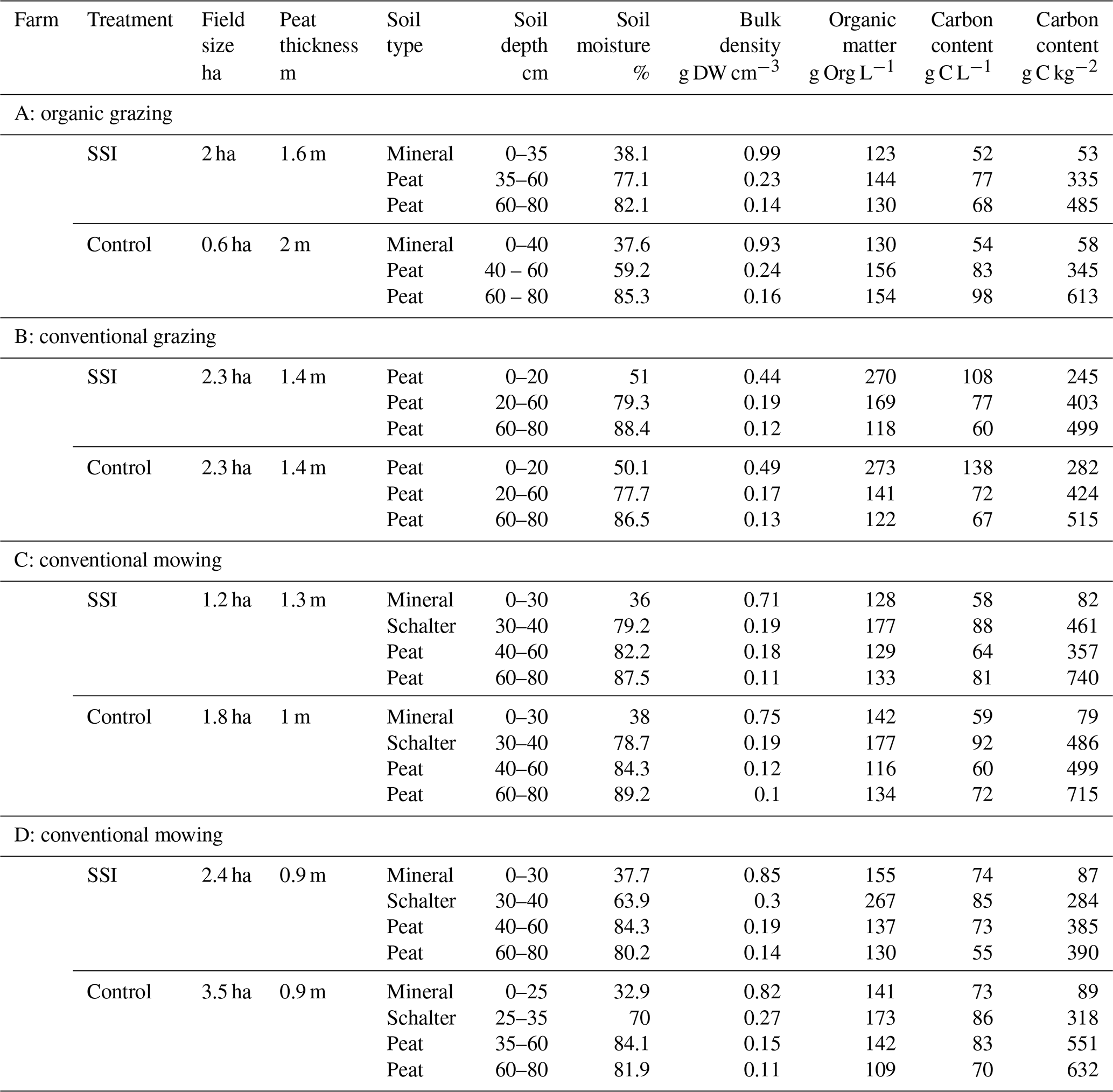
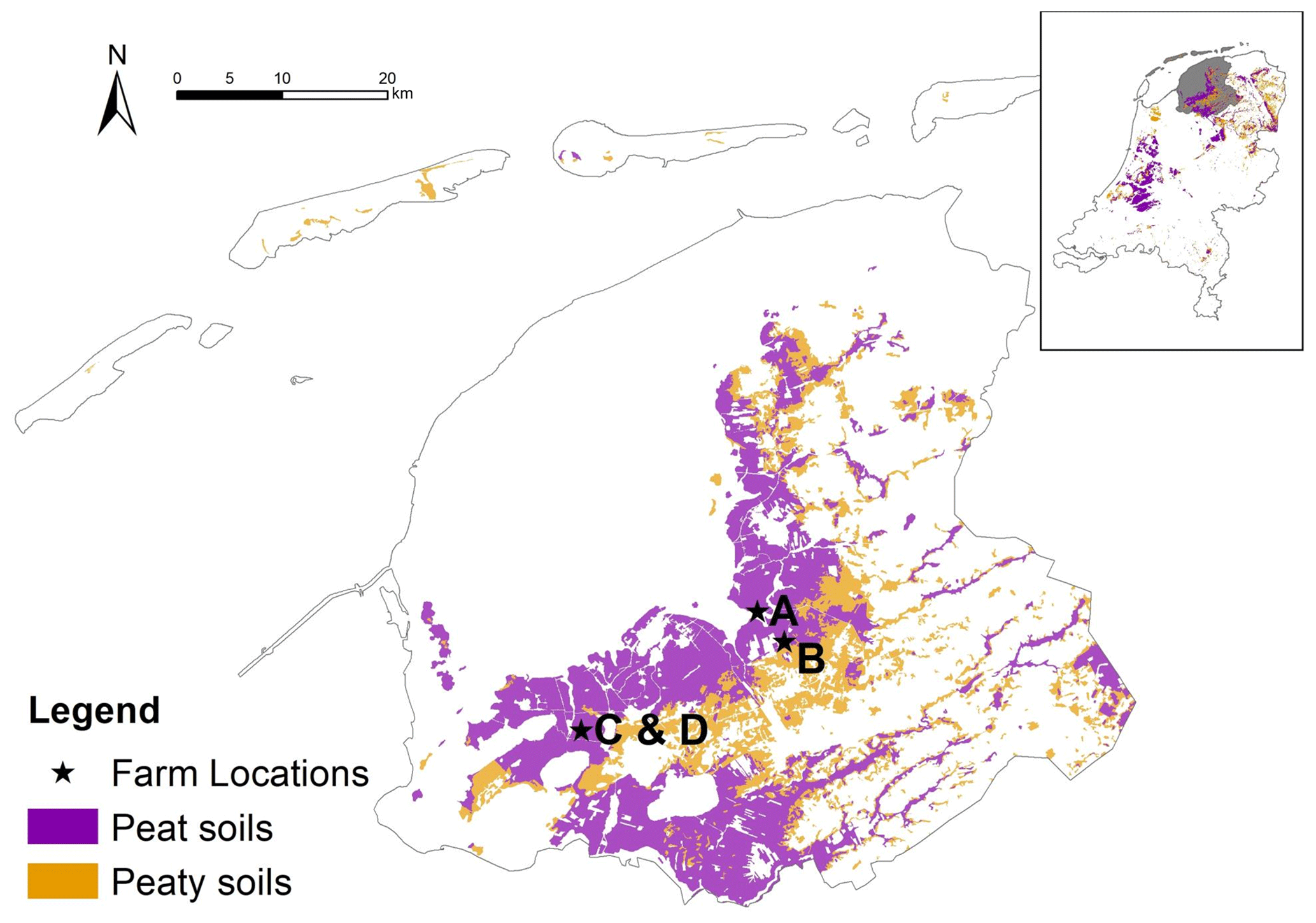
Figure 1Soil map with field locations situated in the province of Friesland, the Netherlands. Peat soils refer to soils with an organic layer of at least 40 cm within the first 120 cm, while peaty soils are soils with an organic layer of 5–40 cm within the first 80 cm.
2.1.1 Experiment setup
Four sites were set up at dairy farms with land management and soil types representative for Friesland (see Table 1 and Fig. 1). Each location consisted of a treatment site with SSI pipes and a control site. The SSI pipes were installed at a depth of 70 cm below the surface and 5–6 m apart from each other, except for the D location where pipes were 5 m apart. The overall drainage intensity was around 2000 m ha−1. The pipes were either directly connected to the ditch (A and C) or connected to a collector tube that was connected to a ditch (B and D). The connections with ditches were placed 10 cm below the targeted ditchwater level that was regulated by a complex network of water inlet and pumps at the lowest parts of the polder. The control sites are fields that have traditional drainage with deep drainage ditches with convex fields and small shallow ditches (furrows).
On the treatment sites, three gas measurement frames 80 × 80 cm were placed for the duration of the experiment on 0.5, 1.5 and 3 m distance from the chosen SSI pipe (Fig. 2), representing best the variation in the environmental conditions and vegetation. The control sites were located 32–42 m from the ditch. Dip well tubes were installed to monitor water tables 0.5, 1.5 and 3 m from the pipe, pairing with the locations of gas measurement frames (Fig. 2). The nylon-coated tubes were 5 cm wide, and perforated filters (130–150 cm length) were placed in the peat layer. The tube 1.5 m from the SSI pipe was equipped with a pressure sensor and a data logger (ElliTrack-D, Leiderdorp Instruments, Leiderdorp, Netherlands) that measures and records the GWT every hour. Ten more dip well tubes were further placed at intervals 0.5 and 3 m from the pipes in the field, which were manually sampled every 2 weeks during gas sampling campaigns, to obtain the variation on the field scale.
To determine soil properties, soil samples were taken using a gouge auger in three replicates until 0.8 m depth and 1.5 m from the SSI pipes taken in August 2017. For soil moisture, sediment samples were weighed and subsequently oven-dried at 105 ∘C for 24 h. Organic matter content was determined via loss on ignition. Dried sediment samples were incinerated for 4 h at 550 ∘C (Heiri et al., 2001). Total nitrogen (TN) and total carbon (TC) was determined in soil material (9–23 mg) using an elemental CNS analyzer (NA 1500, Carlo Erba; Thermo Fisher Scientific, Franklin, USA).
Soil temperature at −5, −10 and −20 cm depth was continuously measured (12 bit temperature sensor S-TMB-M002, Onset Computer Corporation, Bourne, USA) during the run time of the experiment and recorded every 5 min on a data logger (HOBO H21-USB Micro Station, Onset Computer Corporation, Bourne, USA). Because of the frequent failure of sensors, extra temperature sensors (HOBO™ pendant loggers, model UA-002-64, Onset Computer Corporation, Bourne, USA) were placed in the soil at a depth of −5 and −10 cm.
At farms A and D, sensors were set up at 1.5 m above ground to measure photosynthetically active radiation (PAR, smart sensor S-LIA-M003, Onset Computer Corporation, Bourne, USA), air temperature and air relative humidity (temperature/relative humidity smart sensor S-THB-M002, Onset Computer Corporation, Bourne, USA). Data were logged every 5 min (HOBO H21-USB Micro Station, Onset Computer Corporation, Bourne, USA). Average air temperature and precipitation from the weather station Leeuwarden (18 to 30 km distance from research sites) were used (KNMI). The location specific precipitation was estimated using radar images with a resolution of 3×3 km.
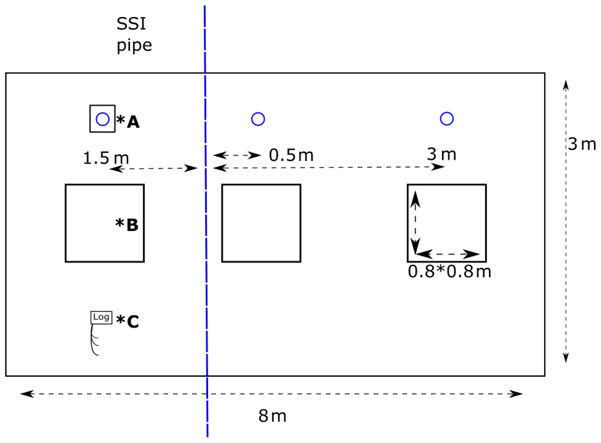
Figure 2Overview field site SSI. Blue dashed line represents the SSI pipe, and the blue circle represents the dip well. *A – dip well with data logger; *B – greenhouse gas flux measurement frame; *C – data logger; −5, −10 and −20 soil temperature.

Figure 3Monthly average air temperature at weather station Leeuwarden (18 to 30 km distance from research sites), and the 30-year average. Sum of monthly precipitation at weather station Leeuwarden, and the 30-year average.
C export from frames used GHG measurements and was determined by harvesting the standing biomass eight times in 2017 and five times in 2018. Two of the harvest moments in 2017 were extra planned – once in May because of the fast grass growth and grass height exceeding 30 cm, and the other in December in order to reset the grass height to the start of the experiment for next year. Surrounding the frames an area of 8×3 m was fenced off to avoid disturbance from grazing and other field activities (Fig. 2). The fenced-off area outside the frames was managed with five cuts per year to have a similar grass height with the farmland. The biomass was harvested, weighed for fresh weight and dried at 70 ∘C until constant weight. Total nitrogen (TN) and total carbon (TC) were determined in dry plant material (3 mg) using an elemental CNS analyzer (NA 1500, Carlo Erba; Thermo Fisher Scientific, Franklin, USA). Due to grazing disturbance in 2018, an estimation instead of measurements was made for the C export of location A in consultation with the farmer but excluded from statistical analysis. Four times per year, slurry manure from location C was applied to all plots. The slurry was diluted with ditchwater (2:1 ratio) and applied above ground in the gas measurement frames and the surrounding area (119–181 kg N ha−1 yr−1 for 2017 and 129–162 kg N ha−1 yr−1 for 2018 with a ratio of 16.3 ± 1.3).
2.2 Flux measurements
CO2 exchange was measured from January 2017 to December 2018, at a frequency of two measurement campaigns a month during growing season (April–October) and once a month during winter. This resulted in 34 (A), 35 (C and D) and 38 (B) campaigns over the 2 years for CO2 and CH4. The N2O emissions were measured with a lower frequency with 22 (A), 20 (B and C) and 17 (D) campaigns over the 2 years. A measurement campaign consisted of flux measurements with opaque (dark) and transparent (light) closed chambers ( m) to be able to distinguish ecosystem respiration (Reco) and gross primary production (GPP) from net ecosystem exchange (NEE). An average of 9 light and 10 dark measurements during winter and 18 light and 20 dark measurements during summer were carried out over the course of the day to achieve data over a gradient in soil temperature and PAR.
The chamber was placed on a frame installed into the soil and connected to a fast greenhouse gas analyzer (GGA) with cavity ring-down spectroscopy (GGA-30EP, Los Gatos Research, Santa Clara, CA, USA) to measure CO2 and CH4 or to a G2508 gas concentration analyzer with cavity ring-down spectroscopy (G2508 CRDS Analyzer, Picarro, Santa Clara, CA, USA) to measure N2O. To prevent heating and to ensure thorough mixing of the air inside the chamber, the chambers were equipped with two fans running continuously during the measurements. For CO2 and CH4, each flux measurement lasted on average 180 s. N2O fluxes were measured on all frames at least once during a measurement campaign, with an opaque chamber for 480 s per flux.

Figure 4Groundwater table (GWT, from soil surface) during the measuring period per farm (letter); values are shown for SSI (measured at 1.5 m from the irrigation pipe) and control treatments.
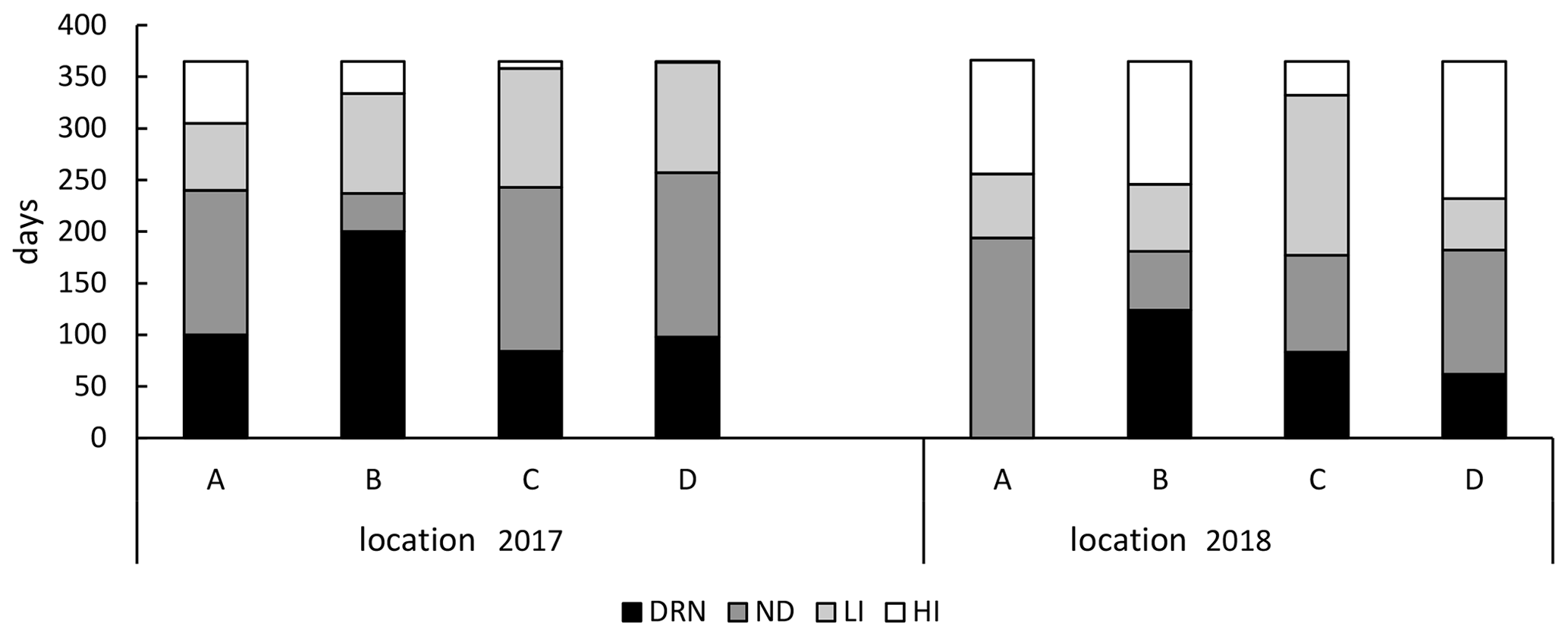
Figure 5Days with effective drainage/irrigation for the four locations: drainage (DRN, < −5 cm), no difference (ND, −5–5 cm), low to intermediate irrigation (LI, 5–20 cm) and high irrigation (HI, > 20 cm) 1.5 m from the SSI pipe.
PAR was manually measured (Skye SKP 215 PAR quantum sensor, Skye instruments Ltd., Llandrindod Wells, United Kingdom) during the transparent measurements on top of the chamber. The PAR value was corrected for transparency of the chamber. Within each measurement, a variation in PAR higher than 75 µmol m−2 s−1 would lead to a restart of the measurement. Soil temperature was measured manually in the frame after the dark measurements at −5 and −10 cm depth (Greisinger GTH 175/PT thermometer, GHM Messtechnik GmbH, Regenstauf, Germany). Grass height was measured using a straight scale with a plastic disk with a diameter of 30 cm before starting the measurement campaign.
2.2.1 Data analyses
2.2.2 Flux calculations
Gas fluxes were calculated using the slope of gas concentration over time (Almeida et al., 2016) (Eq. 1).
where F is gas flux (mg m2 d−1); V is chamber volume (0.32 m3); A is the chamber surface area (0.64 m2); slope is the gas concentration change over time (ppm s−1); P is atmospheric pressure (kPa); F1 is the molecular weight, 44 g mol−1 for CO2 and N2O and 16 g mol−1 for CH4; F2 is the conversion factor of seconds to days; R is the gas constant (8.3144 J K−1 mol−1); and T is temperature in kelvin (K) in the chamber.
2.2.3 Reco modeling
To gap-fill for the days that were not measured for an annual balance for CO2 exchange, Reco and GPP models needed to be fitted with the measured data for each measurement campaign. Reco was fitted with the Lloyd–Taylor function (Lloyd and Taylor, 1994) based on soil temperature (Eq. 2):
where Reco is ecosystems respiration, Reco,Tref is ecosystem respiration at the reference temperature (Tref) of 281.15 K and was fitted for each measurement campaign, E0 is long-term ecosystem sensitivity coefficient (308.56, Lloyd and Taylor, 1994), T0 is temperature between 0 and T (227.13, Lloyd and Taylor, 1994), T is the observed soil temperature (K) at 5 cm depth, and Tref is the reference temperature (283.15 K). If it was not possible to get a significant relationship between the T and the Reco with data from a single campaign, data were pooled for 2 measuring days to achieve significant fitting (Beetz et al., 2013; Poyda et al., 2016; Karki et al., 2019).
2.2.4 GPP modeling
GPP was obtained by subtracting the measured Reco (CO2 flux measured with the dark chambers) from the measured NEE (CO2 flux measured with the light chambers). For the days in between the measurement campaigns, data were modeled with the relationship between the GPP and PAR using a Michaelis–Menten light optimizing response curve (Beetz et al., 2013; Kandel et al., 2016). For each measurement location per measurement campaign, the GPP was modeled by the parameters α and GPPmax (maximum photosynthetic rate with infinite PAR) of Eq. (3):
where GPP is the CO2 flux measured with transparent chambers and corrected with Reco; α is ecosystem quantum yield (mg CO2–C m−2 h−1) (µmol m−2 s−1), which is the linear change of GPP per change in PAR at low light intensities (< 400 µmol m−2 s−1) as in Falge et al. (2001); PAR is measured photosynthetic active radiation (µmol quantum m−2 s−1); and GPPmax is gross primary productivity at its optimum. Due to low coverage of the PAR range in a single measurement campaign, data from multiple campaigns were pooled according to dates, vegetation and air temperature.
2.2.5 Net ecosystem carbon balance calculations
The NEE is the sum of Reco and GPP values, calculated by applying the hourly monitored soil temperature (−5 cm) and PAR data to the models developed per campaign. Extrapolated values at times between two adjacent models are weighted averages of the estimates from these two models, where the weights are temporal distances of the extrapolated time spots to both of the measurements. To account for the influence from plant biomass on the CO2 fluxes, linear relationships between grass height and model parameters (Reco,Tref, GPPmax and α) were developed. Models developed for the campaign before harvesting were then corrected using the slopes of the linear regressions as the models after the harvest to be applied in the extrapolation. The loss of biomass was therefore accounted for according to lowered grass height, which is different from the studies where model parameters are set to zero after harvest (e.g., Beetz et al., 2013). Unrealistic parameters after correction were discarded and instead adopted from parameters from campaigns with low grass height at the same plot. The annual CO2 fluxes were thus the sum of the hourly Reco, GPP and NEE values. The atmospheric sign convention was used for the calculation of NECB. All C fluxes into the ecosystem were defined as negative (uptake from the atmosphere into the ecosystem), and all C fluxes from the ecosystem to the atmosphere are defined as positive. This also holds for non-atmospheric inputs like manure (negative) and outputs like harvests (positive). Both harvest and manure input are expected to be released as CO2.
2.2.6 CH4 and N2O fluxes
CH4 and N2O fluxes per site and measurement campaign were averaged per day. The annual emissions sums for CH4 were estimated by linear interpolation between the single measurement dates. Global warming potential (GWP) of 34 t CO2 eq. for CH4 was used according to IPCC standards (Myhre et al., 2013).
2.2.7 Uncertainties
The estimation of total uncertainties of the yearly budget should include multiple sources of error, where both model error and uncertainty from extrapolations in time are the most important (Beetz et al., 2013). Therefore, we included these two sources of error and combined them into a total uncertainty in three steps. First, we calculated the model error, which would cover the uncertainties from replications (between the three frames) and the random errors from the measurements, the environmental conditions at the time, and the parameter estimation of Reco and GPP. Standard errors (SEs) of the prediction were calculated for each measurement campaign/pooled dataset as the SEs of the midday of the campaign dates. The hourly SEs were then extrapolated linearly between modeled campaigns. Total model error of the annual NEE was therefore calculated following the law of error propagation as the square root of the sum of squared SEs. Second, we attribute the uncertainty from extrapolation to the variations from selecting different gap-filling strategies, since other approaches of annual NEE estimation including different Reco and GPP models would result in different values (Karki et al., 2019). To quantify this uncertainty, six Reco models and four GPP models were selected from Karki et al. (2019) and fitted with annual data (Appendix Table A1). The models were evaluated following the thresholds of performance indicators in Hoffmann et al. (2015). Fitted parameters of Reco and GPP models that performed above the satisfactory rating were accepted and used to gap-fill NEEs. Based on all the annual NEEs per site and year, standard deviations from the means were considered to be the extrapolation uncertainty. In the year 2018, the control site of farm D did not yield any satisfactory Reco models. The uncertainty was thus calculated as the average of all sites. Finally, we calculated the total uncertainties per site and year following the law of error propagation with the uncertainties from the previous steps.
2.3 Statistics
The effect of the treatment on gap-filled annual Reco and GPP, the resulting NEE, the C-export data, the NECB, and the measured CH4 and N2O exchanges were tested by fitting linear mixed-effect models with farm location as a random effect. Effectiveness of the random term was tested using the likelihood ratio test method. The significance of the fixed terms was tested via Satterthwaite's degrees-of-freedom method. General linear regression was used instead when the mixed-effect model gave a singular fit. The treatment effect was further tested using campaign-wise Reco data. Measured Reco fluxes from SSI and control were calculated into daily averages and paired per date. The data pairs were grouped based on the GWT differences between SSI and control of the dates. Differences between treatments were then analyzed by linear regression of the Reco flux pairs without interception and testing the null hypothesis “slope of the regression equals to 1”. All statistical analyses were computed using R version 3.5.3 (R Team Code, 2019) and packages lme4 (Bates et al., 2014), lmerTest (Kuznetsova et al., 2017), sjstats (Lüdecke, 2019) and car (Fox and Weisberg, 2018).
3.1 Weather conditions
Mean annual air temperature was 10.3 ∘C for 2017 and 10.7 ∘C for 2018, which were higher than the 30-year average of 10.1 ∘C. The growing season (April–September) in 2017 was slightly cooler at 14.3 ∘C than the average of 2018 at 14.6 ∘C, while the temperature during the growing season in 2018 was 1.1 ∘C warmer than average. Precipitation was slightly higher for 2017 840–951 mm compared to the 30-year average of 840 mm (KNMI). There was a small period of drought in May and June, ending in the last week of June (See Fig. 3). In contrast, 2018 was a dry year with average precipitation of 546–611 mm (range of two sites in Friesland). The year is characterized by a period of extreme drought in the summer, from June to the beginning of August, and precipitation lower than average in the fall and winter.
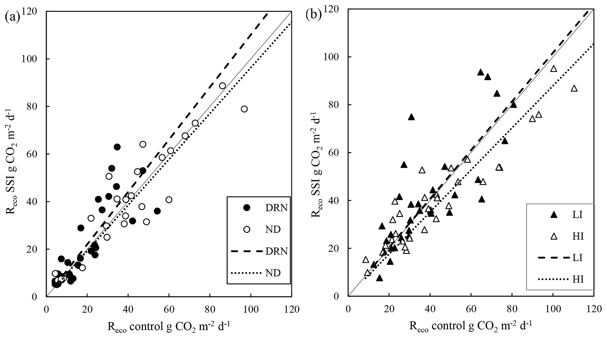
Figure 6Measured fluxes for ecosystem respiration (Reco), one-to-one comparison in which daily averages were used. (a) Values are divided into two groups: with lowered groundwater table due to the effect of drainage (DRN) and with a small difference (ND). (b) Values are divided into two groups with irrigation effects: moderate infiltration with more than 5–20 cm difference (LI) and high infiltration (HI) with more than 20 cm difference between SSI and control. The black filled line is the 1:1 line.
Table 2Average groundwater table (cm from the surface level) during the measuring period per farm. Summer groundwater table ranges from April until October. Measured 1.5 m from the SSI pipe.

3.2 Groundwater table (GWT)
Deploying SSI systems affected GWT dynamics during the 2 years for all farms (Fig. 4). However, there was a large variation in effect size between years and locations. The effect of SSI can be divided into two types of periods. Periods with drainage (decreased GWT), in the wet periods, coincided with the autumn (in 2017) and winter period (2017 and 2018). Irrigation (increased GWT) periods, where the SSI leads to a higher water table than control, occurred during spring and summer when the GWT dipped below the ditch water level. In 2017, the effectiveness differed per farm. For locations A and B, GWT was more stable in summer around the −60 and −70 cm for SSI compared to the control, while for locations C and D the GWT fluctuated more like in the control fields. During the dry summer of 2018, in contrast, all locations showed a strong effect of irrigation, especially after the dry period in the beginning of August. In this period the water table recovered quickly while the control lagged behind.
Table 3Overview of all processes contributing to the carbon balance calculated for both years. Ecosystem respiration (Reco), gross primary production (GPP), net ecosystems exchange (NEE, sum of GPP and Reco), C exports (harvest), C manure (carbon addition from manure application), and net ecosystem carbon balance (NECB, sum of all fluxes) for subsoil irrigation (SSI) and control plots at farm locations A–D. The range of Reco, GPP and NEE represent the combination of model error and extrapolation uncertainties following the law of error propagation.
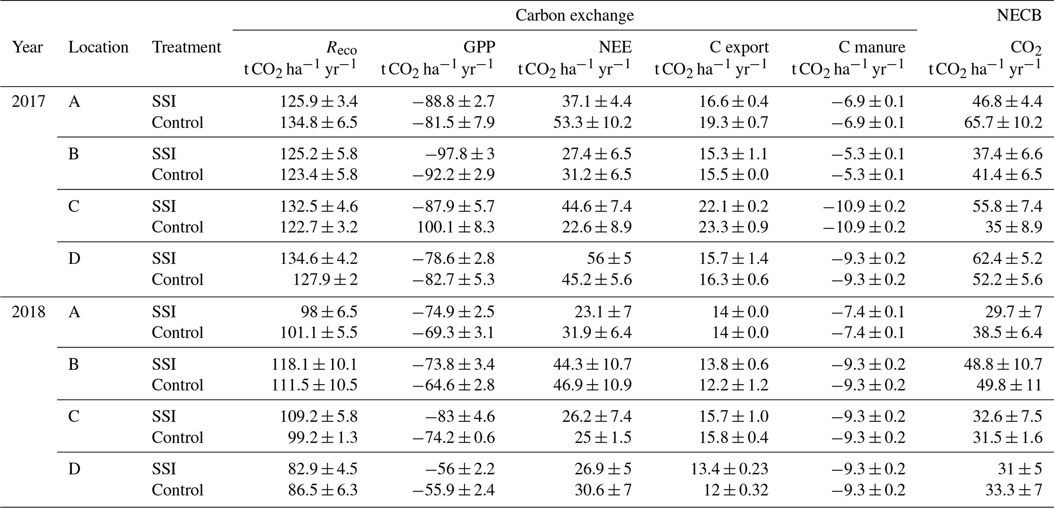
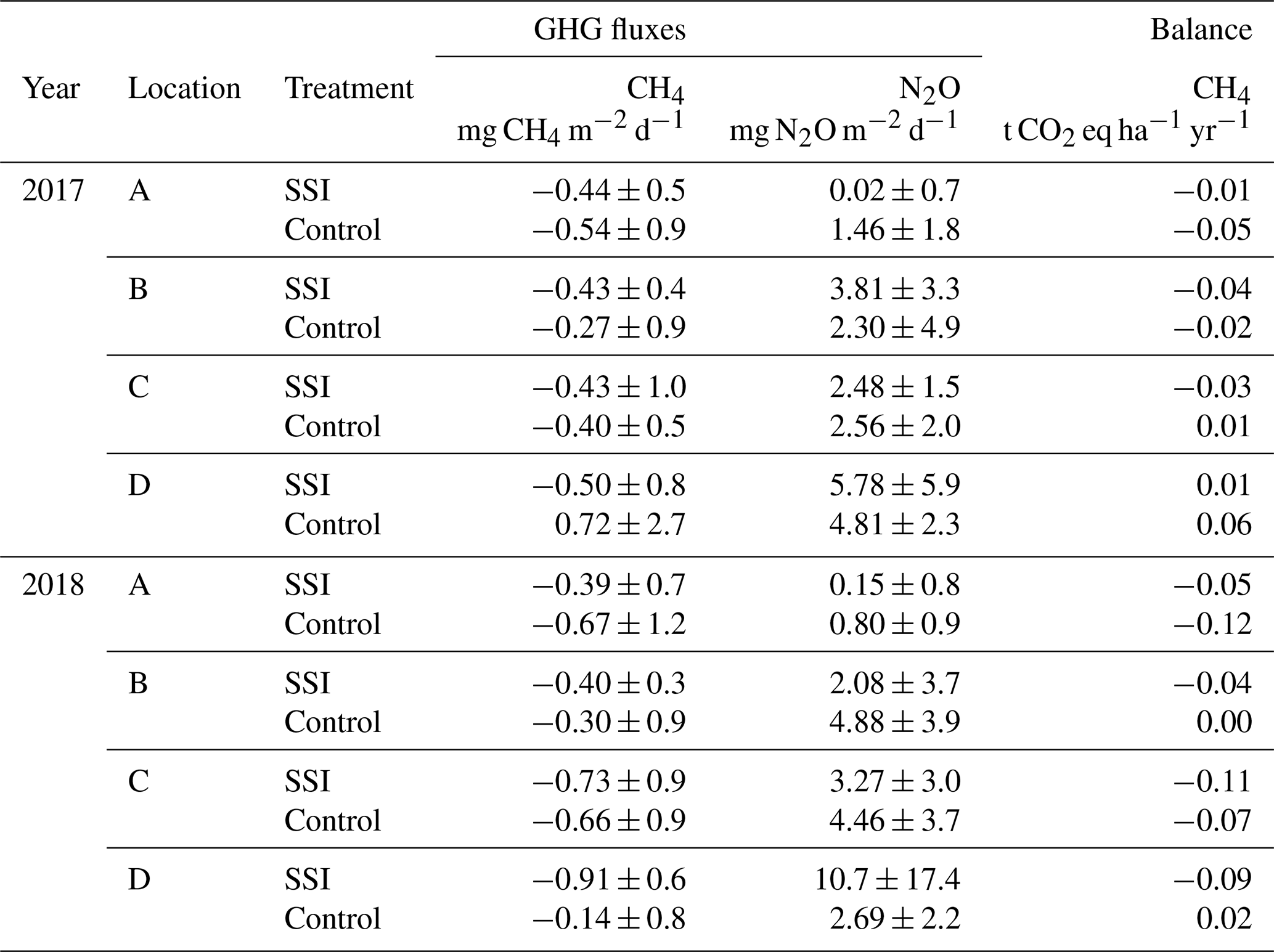
Table 4The average measured CH4 and N2O emissions subsoil irrigation (SSI) and controls for the four locations (A–D) for both years in mg m−2 d−1. The total CH4 balance in CO2 equivalents, using radiative forcing factors of 34 for CH4 according to IPCC standards (Myhre et al., 2013). The ranges of CH4 and N2O represent the standard deviation (SD) of the measured fluxes.
Although there was hardly any difference in annual average GWT between control and SSI (< 5 cm; Table 2), drainage and irrigation effects could be observed when dividing the calendar year into seasons. The effective days of the SSI are summarized in Fig. 5 according to four classes, based on practical definitions of drainage and irrigation: drainage (DRN, < −5 cm), no difference (ND, −5–5 cm), low to intermediate irrigation (LI, 5–20 cm) and high irrigation (HI, > 20 cm). These classes are also used in the statistical analysis of Reco measurements (see Sect. 3.3, measured Reco). In 2017 there were 17 d more without any GWT difference than in 2018. There was a much stronger irrigation effect in the dry year of 2018, with 61 more irrigated days comparing to 2017, and the number of irrigation days was constantly similar to, or higher than, the number of drainage days, except for site B in 2017, which had a long period showing a drainage effect.
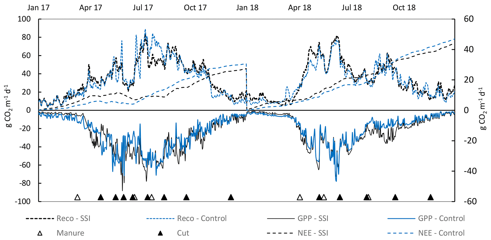
Figure 7Reco and GPP for location B in g CO2 m−2 d−1 on the primary y axis, for control and SSI. Accumulative NEE in t CO2 ha−1 yr−1, for control and subsoil irrigation (SSI), every year starting at 0.
3.3 Measured Reco
Figure 6 compares the measured Reco fluxes with the corresponding GWT measurements, which could give an indication for the effectiveness of the GWT differences. The classes were based on the GWT differences between the SSI and control sites on the measurement days (the same classes used in Fig. 5). There was a slightly higher Reco for SSI during drainage periods when GWT was lower (DRN), which compensates for the lower Reco during summer. For moments where there was no GWT difference (ND) and those showing moderate irrigation (LI), there was no effect of SSI on Reco. However, when the GWT of the SSI was more than 20 cm higher than the control (HI), the emissions of the control were significantly higher than SSI (p < 0.01), indicating an effect of the irrigation. However, this effect of the raised GWT was small, even though in some cases the GWT was raised more than 60 cm. According to Fig. 5, in 2017, the majority of the days were dominated by drainage (increasing Reco) or by no difference or small irrigation resulting in no effect on the Reco. However, periods with increased irrigation (Fig. 5), when there was a reduced Reco effect of SSI, were sparse compared to the other dominating periods.
3.4 Annual carbon fluxes
3.4.1 Gross primary production (GPP)
GPP was high for all locations in both years, showing a clear seasonal pattern with the highest uptake at the start of the summer (Fig. 7). GPP was 30 % lower in the dry year 2018 (p < 0.001) compared to 2017 (see Table 2) and differed between locations (random effect p = 0.006). There was, however, no treatment effect on GPP (p = 0.3101). Average GPP values for all SSI and control plots were −88.3 ± 7.5 and −89.2 ± 13 t CO2 ha−1 yr−1 for 2017 and −71.7 ± 6.6 and −65.7 ± 4.9 t CO2 ha−1 yr−1 for 2018, respectively.
3.4.2 Ecosystem respiration (Reco)
Reco was generally high for all the farms measured during the 2 years, with the average Reco of 128.4 ± 4.6 t CO2 ha−1 yr−1 for 2017 being significantly higher than 100.8 ± 11 t CO2 ha−1 yr−1 for 2018 (p < 0.001) (Table 2). Different seasonal patterns were also observed between the 2 years, where in 2017 Reco peaked in June and July, while in 2018 the highest Reco was found in May (Fig. 7, Appendix B). However, no effect of SSI on Reco was found (p = 0.6191), with average Reco values for all SSI and control plots of 128.7 ± 9.2 and 126.7 ± 9.5 t CO2 ha−1 yr−1 in 2017 and 102.1 ± 14.1 and 99.6 ± 13.5 t CO2 ha−1 yr−1 in 2018.
3.4.3 Net ecosystem exchange (NEE)
All locations functioned as large C sources during the measurement period. The average annual NEE of all sites amounted to 39.7 ± 11 and 31.8 ± 8.4 t CO2 ha−1 yr−1 in 2017 and 2018, respectively. The overall explanatory power of year, treatment and location was low, with no yearly difference between 2017 and 2018 (p = 0.1813), or any treatment effect of SSI (p = 0.9805). The average NEE values for all SSI and control plots are 40.4 ± 11.9 and 37.5 ± 16.1 t CO2 ha−1 yr−1 in 2017 and 30.4 ± 15.6 and 34 ± 14.5 t CO2 ha−1 yr−1 in 2018, respectively.
3.4.4 C export (yield)
C exports (i.e., yields) differed between years without treatment effect of SSI (p = 0.691). Following the drought in 2018, C export (13.8 ± 0.6 t CO2 ha−1 yr−1) was significantly lower (p < 0.001) than in 2017 (18.0 ± 1.4 t CO2 ha−1 yr−1). These values corresponded to dry matter (DM) yields of 9.4 ± 0.6 t DM ha−1 yr−1 in 2018 and 12.6 ± 1.1 t DM ha−1 yr−1 in 2017. The year effect differed per location (random effect p < 0.001). We found a solid relationship between C export and GPP (p < 0.001, r2=0.942; linear mixed-effect modeling).
3.4.5 Net ecosystem carbon balance (NECB)
All sites are large carbon sources, without an effect from SSI (p = 0.9446), which was consistent for all farms (Table 3). However, there was a significant difference between the 2 years, with higher C emission rates in 2017 amounting to 49.6 ± 11 t CO2 eq. ha−1 yr−1 on average, compared to 36.9 ± 7.6 t CO2 eq. ha−1 yr−1 for 2018 (p=0.0277).
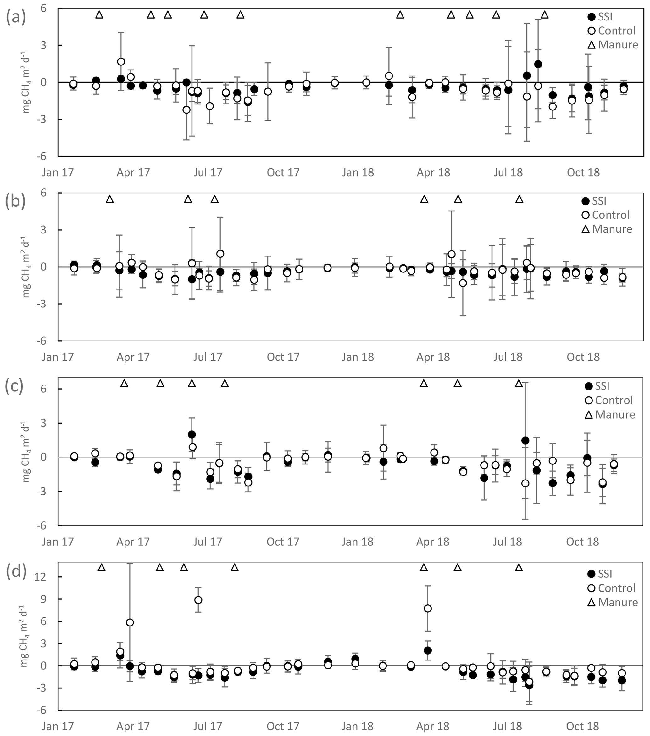
3.5 Methane exchange
The total exchange of CH4 was very low during both years, with no effect from the SSI (p=0.1147) or difference between years (p=0.1253). During most periods, the locations functioned as a sink of CH4. The annual fluxes were −0.01 ± 0.01 t CO2 eq. ha−1 yr−1 (−0.25 kg CH4 ha−1 yr−1) for 2017 and −0.06 ± 0.05 t CO2 eq. ha−1 yr−1 (−1.8 kg CH4 ha−1 yr−1) for 2018 (Table 4). Such exchange did not play a significant part in the total GHG emissions (comparable to less than 0.4 % of the annual NECB).
3.6 Nitrous oxide exchange
There was no treatment effect (p=0.5640) or inter-annual difference (p=0.4414) detected. The highest average emissions were measured on the SSI plot of location D, with 5.78 ± 5.9 mg N2O m−2 d−1 for 2017 and 10.7 ± 17.4 mg N2O m−2 d−1 for 2018. The highest peak was measured on the frame closest to the SSI pipe in August for SSI of location D, showing 55 ± 15 mg N2O m−2 d−1. The peaks observed were erratic and did not correspond to fertilization management with slurry before measurement campaigns.
In this experimental research we found effects of subsoil irrigation (SSI) on water table dynamics without changing carbon dynamics profoundly. For both years, SSI had a clear irrigation effect during summer, increasing the averages of GWT during the summer period by 6–18 cm at the four farms. During winter, there was a moderate but consistent drainage effect, reducing the average GWT in the wet/winter period by 1–20 cm. Mean annual GWT was little affected by SSI. Despite the irrigation effects and higher water tables in summer, there was no effect of SSI on Reco, GPP and NEE in either of the 2 years. We found no evidence for a reduction of CO2 emissions, or for yield improvements, on an annual base by implementing SSI.
4.1 SSI does not reduce annual Reco
We identified three conditions that can explain the limited effect of SSI on carbon fluxes from the most prominent peat decomposition processes. Firstly, the uppermost 30–40 cm of the soil remains drained in both treatments throughout large parts of the year (220–255 d), facilitating high CO2 fluxes. Secondly, gas exchange from lower soil layers (60 cm and below) was presumably low due to moisture levels close to saturation that limit diffusion of CO2 and O2 effectively. Thirdly, the deliberate increase in drainage in the SSI treatment frustrates the irrigation effect on GWT. As a consequence, mean annual GWT was similar for both treatments.
Based on the direct comparison using measured Reco fluxes (Fig. 6), we found a modest 5 %–10 % reduction in Reco only when GWT differences were larger than 20 cm. When the irrigation effect was smaller, no effect on the Reco was found. An earlier study on intensively managed peat pastures in the Netherlands and on the role of GWT also showed small effects of higher summer GWT on annual Reco and NEE despite substantial differences in soil volume changes/soil subsidence (Dirks et al., 2000). Similarly, a 4-year study (Schrier-Uijl et al., 2014) found little differences in NEE estimates despite substantial variations in summer GWT and soil moisture contents.
It is generally assumed that higher GWT (mean annual or actual) leads to lower CO2 emissions according to laboratory data (Moore and Dalva, 1993) and correlations between annual CO2 fluxes and mean annual GWT (Wilson et al., 2016; Tiemeyer et al., 2020). However, there are also studies that did not find an effect of GWT on CO2 emissions during the growing season (Lafleur et al., 2005; Nieveen et al., 2005; Parmentier et al., 2009). This lack of effect is explained by the fact that there is only a small difference in soil moisture values above the GWT. The lower CO2 emissions reported with structurally elevated GWT are often concomitant with substantial differences in vegetation/land use that are adapted to the higher GWT (Beetz et al., 2013; Schrier-Uijl et al., 2014; Wilson et al., 2016), which could confound the effects of GWT change. In our study, SSI seems to have an effect of a similar magnitude trending towards higher emissions during periods with lower GWT at the SSI sites.
The small treatment effect on measured Reco (Fig. 6) in our study can most probably be explained by differences in peat oxidation rates along the soil profile. Some other studies suggest that the top 30–40 cm of the peat profile play an important role in C turnover rates in drained peatlands, due to more readily decomposable C sources and higher temperatures (Moore and Dalva, 1993; Lafleur et al., 2005; Karki et al., 2016; Säurich et al., 2019). This soil layer was, however, not affected by higher summer GWTs in our study. SSI even reduced the number of days (24–27 d) that the top 30–40 cm soil layer remained saturated, mostly in the wet season. Moreover, Säurich et al. (2019) speculated that the highest CO2 production in the top 10 cm is reached when GWTs are approximately 40 cm below the surface. As the infiltrating water will affect the soil moisture content of these layers, it is possible that SSI could even facilitate rather than mitigate summer emissions by approaching the optimum for C mineralization more often.
In contrast to surface irrigation, where the topsoil is replenished with moisture, the SSI effect is limited to deeper parts of the peat soils, at −60–100 cm depth. However, the role of this deeper layer as a prominent C source for emissions to the atmosphere is likely to be limited. CO2 production and export from deeper layers is prevented by lower temperatures, limited O2 intrusion and the fact that water content of this layer is already close to saturation, which is frustrating gas diffusion (Berglund and Berglund, 2011; Taggart et al., 2012; Säurich et al., 2019). This layer shows low levels of stronger electron acceptors such as O2 and nitrate used for the microbial oxidation of organic compounds and of labile organic matter (Fontaine et al., 2007; Leifeld et al., 2012). Visually, the layers at our sites deeper than 60 cm were less decomposed (yellow–brown color with plant macrofossils still visible) compared to the highly degraded peat in the uppermost 40 cm layer.
In our case, although CO2 production in deeper peat layers could be lower due to saturation after SSI induced GWT elevation, this reduction may be compensated for by the increased CO2 production in the top 20–40 cm due to the higher moisture levels resulting from elevated water levels. In the dry year of 2018, large differences between GWT in SSI and control sites of up to 20 cm were observed, with the lowest summer GWT as deep as −120 cm in the control sites. A maximized effect of SSI would be expected according to the assumption from the Dutch soil–carbon–water model, where the average lowest summer GWT (i.e., GLG “gemiddeld laagste grondwaterstanden”) is considered to be the major control of CO2 emissions (STOWA, 2020). The absence of an SSI treatment effect in this case provides additional evidence that SSI contributes little if any to the mitigation of CO2 emission from drained peatlands. Such understanding of the processes of CO2 emissions in relation to soil profiles should be further investigated.
4.2 SSI effects on CH4 and N2O emission
The magnitudes of measured CH4 and N2O fluxes are substantially lower than CO2 fluxes, which would thus lead to negligible contributions to the total GHG emissions in our case. Looking directly at the measured fluxes, no SSI effect was detected for either CH4 or N2O. Findings of this experiment agree with the generally accepted idea that intensively drained peatlands have low levels of CH4 emissions, and often these systems even function as a small CH4 sink (Couwenberg et al., 2011; Couwenberg and Fritz, 2012; Tiemeyer et al., 2016; Maljanen et al., 2010). Drainage ditches, in contrast, emitted CH4 at high rates (Kosten et al., 2018; Lovelock et al., 2019). In the current study, the average of all measured N2O fluxes was 3.3 mg N2O m−2 d−1 (12 kg N2O ha−1 yr−1), which falls within the range of annual N2O emissions from drained peatlands in northwest Europe (4–18 kg N2O ha−1) (Leahy et al., 2004; Maljanen et al., 2010; Schrier-Uijl et al., 2014; Kandel et al., 2018). Fertilization, temperature and water table fluctuations play major roles in the total N2O emission (Regina et al., 1999; Van Beek et al., 2011; Poyda et al., 2016). The mechanisms of N2O production and consumption in organic soils are, however, complex, and there is high temporal and spatial variability as influenced by site conditions and management (Leppelt et al., 2014; Taghizadeh-Toosi et al., 2019). It is well known from previous studies that periods with frost and thawing result in high N2O emissions (Koponen and Martikainen, 2004). In this study, the low measurement frequency in both years does not allow annual estimations of N2O with enough representation of peak N2O emission. However, an SSI effect still cannot be expected according to the direct comparison of measured fluxes.
4.3 Reasonably high NEE
In contrast to the expected function of the SSI technique based on land subsidence data, no effect has been found on either promoting the yield/GPP or reducing NEE and other GHG emissions. Our NEE estimate averaging all sites and years at 35.8 (22.6–56.0) t CO2 ha−1 yr−1 is at the higher end of the ranges reported for drained temperate peatlands (Wilson et al., 2016). Tiemeyer et al. (2020) reported 30.4 (5.1–40.3) t CO2 ha−1 yr−1 for drained organic soils in Germany. In a Dutch case study authors found a NECB of 20.1 t CO2 ha−1 yr−1 average over the years 2005–2008 (Schrier-Uijl et al., 2014). Comparing GPP and Reco estimates with earlier reports we find that GPP of the sites was higher than values found by Tiemeyer et al. (2016) for productive and drained peatlands (−70 ± 18 t CO2 ha−1 yr−1), especially in the year 2017 (−88.7 ± 7.2 t CO2 ha−1 yr−1), and falls back to the range in 2018 (−69.0 ± 8.9 t CO2 ha−1 yr−1) due to the drought-induced decline of CO2 uptake (Fu et al., 2020). Higher GPP estimates seem reasonable given the high C export in 2017 (on average 18.0 t CO2 ha−1), which was substantially larger than the 8.5 t CO2 ha−1 reported by Tiemeyer et al. (2016) for grassland on organic soils. On the other hand, the Reco values of the sites (128.4 ± 4.6 and 100.8 ± 11 t CO2 ha−1 yr−1 in 2017 and 2018, respectively) are also at the higher end of the range (97 ± 33 t CO2 ha−1 yr−1 in Tiemeyer et al., 2016). Extrapolation bias was excluded as a possible reason for this high CO2 emission, since testing of different Reco modeling approaches (including different model selection, data clustering procedure and removal of raw data outliers) did not yield substantially different Reco values.
High Reco values may partly be explained by the timing of our measurements. Järveoja et al. (2020) reported in a boreal natural peatland strong diel patterns of Reco with peaks at both midnight and midday. The authors show that daily carbon fluxes were overestimated when models were developed including peak emission. If a similar pattern of Reco applies to temperate highly productive and drained peatlands, the flux measurements with opaque chambers to estimate Reco would need to be spread more evenly during day (and ideally throughout the night). In our case, the flux measurements were unevenly distributed and concentrated around midday, which may have led to overestimation of Reco and, therefore, NEE overestimation. Assuming a structural overestimation of Reco by 15 % results in lower NECB estimates (26 t CO2 ha−1 yr−1) over all sites and both years.
Besides general methodological limitations of the closed-chamber method, there are also a number of biochemical mechanisms that may explain the high emissions found here. Abiotic conditions that favor high CO2 emissions were present, with high temperatures for both years and non-limiting moisture conditions for 2017. Research from Pohl et al. (2015) found in a drained peatland a high impact of dynamic soil organic carbon (SOC) and N stocks in the aerobic zone on CO2 fluxes. In our case, the peat soils contained a high amount of C, especially in the upper 20 cm layer. This layer was also aerobic for long periods during the experiment, thus promoting high rates of C sequestration and decomposition. In conclusion, NEE estimates in the current study are high owing to systemic overestimation of Reco and conditions promoting high soil CO2 production and release.
4.4 Uncertainties
GHG emissions from peat grasslands are highly variable (Tiemeyer et al., 2016) given the uncertainties from the wide ranges of land use and management activities (Renou-Wilson et al., 2016) and gap-filling techniques (Huth et al., 2017). In this study, besides the model errors inherent in the model development process, uncertainties from gap-filling techniques in terms of data-pooling strategies and model selections were also considered. Campaign-wise fitting of Reco and GPP models can best represent the original datasets, while pooling data for a longer period can provide better model fitness and less bias toward single measurements (Huth et al., 2017; Poyda et al., 2017). However, in this study, different responses of vegetation and soil processes to drought, especially to the extreme drought in 2018, caused data points that could not be explained by the classic models, resulting in the generally poor performances of annual models. For this reason, we reported the annual budgets with campaign-wise gap-filled NEE values. The uncertainties of NEE estimates from model differences were on average 14 t and up to 25 t of CO2. Nevertheless, no SSI effect was found considering NEE estimates from annual models. The model differences quantified here were in good agreements with other model tests (Görres et al., 2014; Karki et al., 2019) and match the magnitude of NEE uncertainties calculated with other methods (e.g., the 23–30 t CO2 variances reported by Schrier-Uijl et al., 2014, using eddy co-variance techniques). Additionally, CO2 fluxes and annual budgets derived from the eddy co-variance approach in 2019 at location A support the findings of the present study (Van den Berg and Kruijt, 2020). The eddy co-variance revealed virtually identical flux patterns for both the control and SSI field despite drastic differences in summer GWT surpassing 80 cm at the height of the vegetation period.
4.5 The effects of SSI on land use
The intensity of land use (intensity and timing of drainage and fertilization, plant species composition, mowing and grazing regimes) is a major driver of carbon turnover in grasslands (Renou-Wilson et al., 2016; Smith, 2014; Ward et al., 2016). SSI facilitates earlier fertilization compared to management under current drainage systems by increasing the load-bearing capacity of the field surface for fertilizing equipment. We expect nutrient accumulation in the soil to continue, which can lead to high CO2 losses accelerated by nitrogen or phosphorus (Tiemeyer et al., 2016; Säurich et al., 2019). It was expected that C export via crop yields due to extra drainage could increase in a wet autumn. However, we did not find any indication for an increase in land-use intensity or yield as a result of SSI. In summary, land-use intensity will remain high in SSI treatments without substantial changes to carbon-sequestrating vegetation (e.g., Couwenberg et al., 2011; Schrier-Uijl et al., 2014; Tiemeyer et al., 2020), tillage (Smith, 2014) or fertilization (Pohl et al., 2015).
The implementation of SSI may further inflict high costs on land users. Next to investing in 1800 to 2500 m of extra drainage pipes per hectare the maintenance costs of the fields rise due to additional drainage pipes. Drainage pipe inspection, cleaning and maintenance costs range between EUR 0.30 to 0.90 m−1 with a recurring interval of 3–6 years depending on abiotic conditions (Klaas Kooistra, personal communication, 2020). SSI inflicts practical challenges in all catchments where ditch water levels are difficult to control and where water needs to be pumped in during summer. Groundwater extraction has been suggested as an alternative which will further increase direct costs (pumping infrastructure, fuel) and indirect costs, including land subsidence following groundwater extraction (Herrera-García et al., 2021). A large roll out of SSI seems costly, is impractical and holds only few benefits for land use on peatlands.
The implementation of the SSI technique with the current design does not lead to a reduction of GHG emissions from drained peat meadows, even though there was a clear increase in GWT during summer (especially in the dry year of 2018). We therefore conclude that the current use of SSI with the aim to raise the water table to −60 cm is ineffective as a mitigation measure to sufficiently lower peat oxidation rates and, therefore, also soil subsidence. Most likely, the largest part of the peat oxidation takes place in the top 40 cm of the soil, which remained drained. This layer is still exposed to higher temperatures, sufficient moisture, oxygen and alternative electron acceptors such as nitrate, and nutrient input. We expect that SSI may only be effective when the GWT can be raised permanently to water tables close to the soil surface.
Table A1Model selected for annual-model gap-filling approach of yearly budgets (adopted from Karki et al. 2019), as a measure of extrapolation uncertainties.
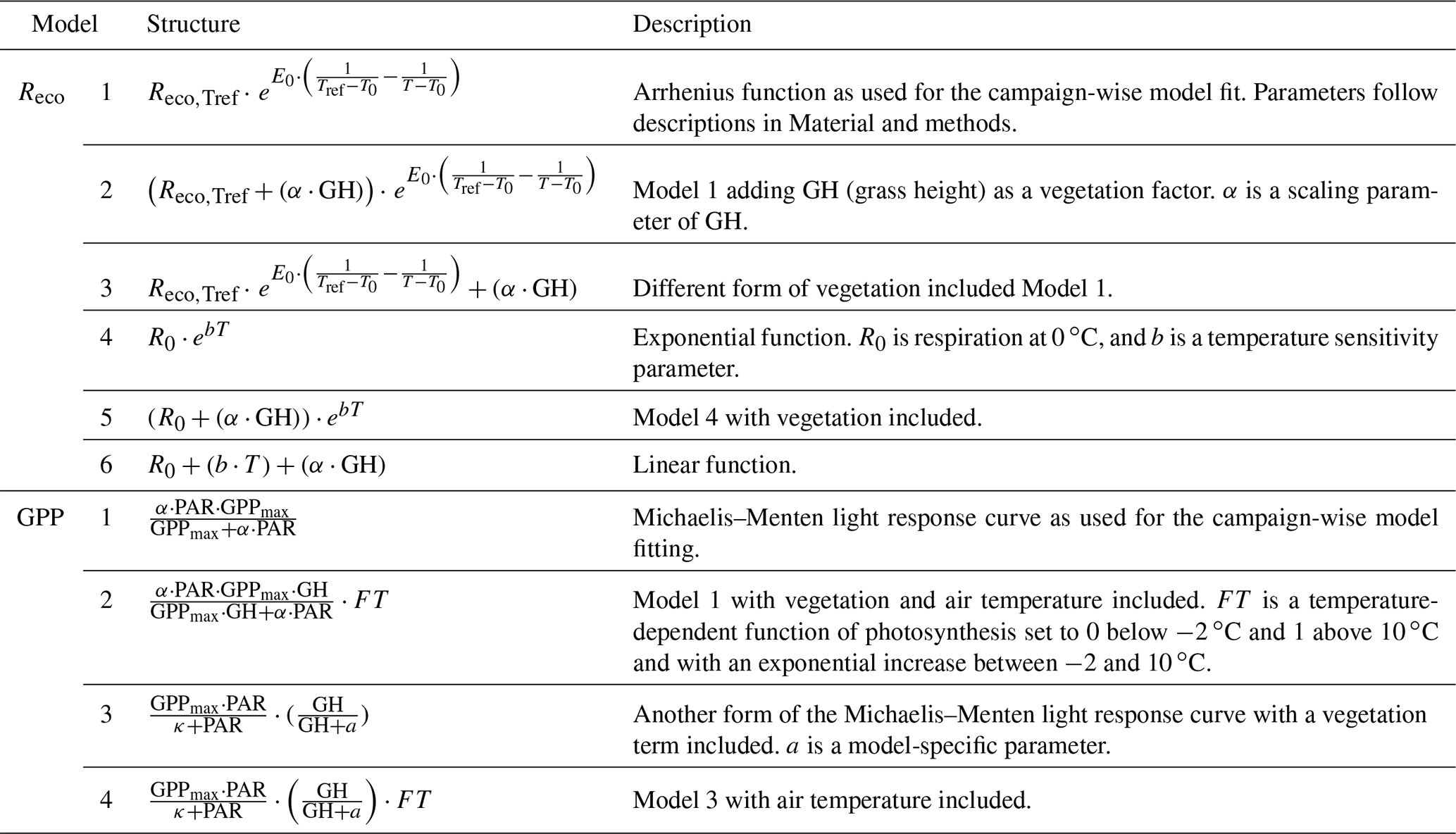
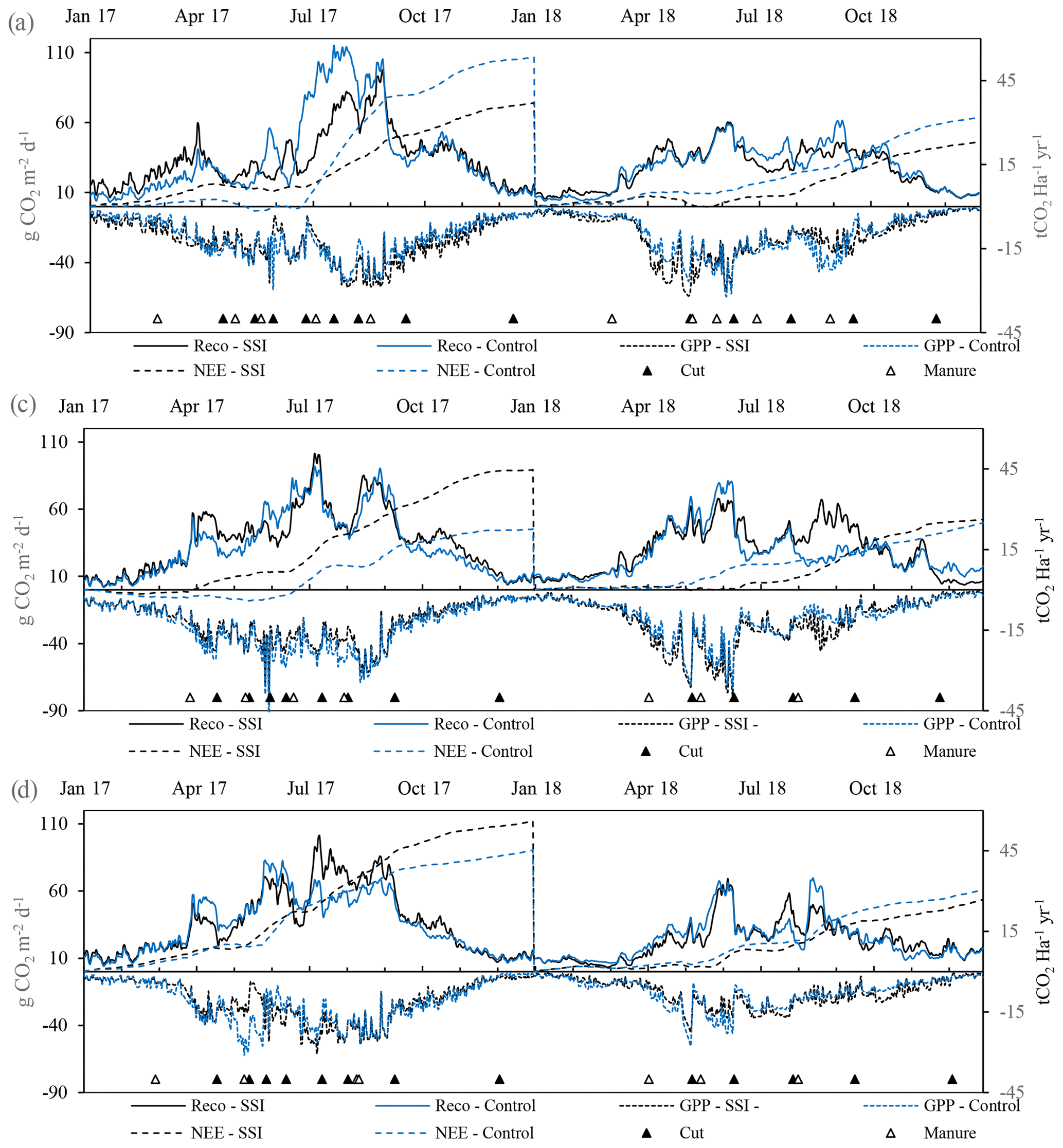
Figure B1Daily Reco and GPP for location in g CO2 m−1 d−1 on the primary y axis, for control and SSI for locations A, C and D. Accumulative NEE in t CO2 ha−1 yr−1, for control and SSI, every year starting at 0.

The data are available on request from the corresponding author (stefan.weideveld1@gmail.com, s.weideveld@science.ru.nl).
CF conceived the presented study. STJW and CF planned and set up the experiment. STJW carried out the experiment with support from WL, MB and CF. STJW, WL and MB processed the experimental data, performed the analysis and designed the figures. STJW, WL, MB, and CF drafted the manuscript with support from LPML. CF and LPML supervised the project.
The authors declare that they have no conflict of interest.
We would like to thank all technical staff, students and others who helped in the field and in the laboratory, as well as the landowners who granted access to the measurement sites. We acknowledge Peter Cruijsen and Roy Peters for their assistance in practical work and analyses.
Weier Liu is supported by the China Scholarship Council (grant no. 201706350201). Merit van den Berg was supported by the NWO Peatwise grant (grant no. ALW.GAS.4). Christian Fritz received funding from FACCE ERA Net+ “Climate Smart Agriculture” (EU) NWO-ALW (CINDERELLA).
This paper was edited by Kees Jan van Groenigen and reviewed by two anonymous referees.
Almeida, R. M., Nóbrega, G. N., Junger, P. C., Figueiredo, A. V., Andrade, A. S., de Moura, C. G., Tonetta, D., Oliveira Jr, E. S., Araújo, F., and Rust, F.: High primary production contrasts with intense carbon emission in a eutrophic tropical reservoir, Front. Microbiol., 7, 1–13, https://doi.org/10.3389/fmicb.2016.00717, 2016.
Arets, E. J. M. M., Van Der Kolk, J., Hengeveld, G. M., Lesschen, J. P., Kramer, H., Kuikman, P., and Schelhaas, N.: Greenhouse gas reporting for the LULUCFsector in the Netherlands: methodological background, update 2020, Statutory Research Tasks Unit for Nature and the Environment, 2352–2739, 2020.
Bates, D., Mächler, M., Bolker, B., and Walker, S.: Fitting linear mixed-effects models using lme4, arXiv preprint, arXiv:1406.5823, 2014.
Beetz, S., Liebersbach, H., Glatzel, S., Jurasinski, G., Buczko, U., and Höper, H.: Effects of land use intensity on the full greenhouse gas balance in an Atlantic peat bog, Biogeosciences, 10, 1067–1082, https://doi.org/10.5194/bg-10-1067-2013, 2013.
Berglund, Ö. and Berglund, K.: Influence of water table level and soil properties on emissions of greenhouse gases from cultivated peat soil, Soil Biol. Biochem., 43, 923–931, 2011.
Brouns, K., Eikelboom, T., Jansen, P. C., Janssen, R., Kwakernaak, C., van den Akker, J. J., and Verhoeven, J. T.: Spatial analysis of soil subsidence in peat meadow areas in Friesland in relation to land and water management, climate change, and adaptation, Environ. Manage., 55, 360–372, 2015.
Couwenberg, J. and Fritz, C.: Towards developing IPCC methane “emission factors” for peatlands (organic soils), Mires Peat, 10, 1–17, 2012.
Couwenberg, J., Thiele, A., Tanneberger, F., Augustin, J., Bärisch, S., Dubovik, D., Liashchynskaya, N., Michaelis, D., Minke, M., and Skuratovich, A.: Assessing greenhouse gas emissions from peatlands using vegetation as a proxy, Hydrobiologia, 674, 67–89, 2011.
Dawson, Q., Kechavarzi, C., Leeds-Harrison, P., and Burton, R.: Subsidence and degradation of agricultural peatlands in the Fenlands of Norfolk, UK, Geoderma, 154, 181–187, 2010.
Dirks, B., Hensen, A., and Goudriaan, J.: Effect of drainage on CO2 exchange patterns in an intensively managed peat pasture, Clim. Res., 14, 57–63, 2000.
Erkens, G., van der Meulen, M. J., and Middelkoop, H.: Double trouble: subsidence and CO2 respiration due to 1,000 years of Dutch coastal peatlands cultivation, Hydrogeol. J., 24, 551–568, 2016.
Falge, E., Baldocchi, D., Olson, R., Anthoni, P., Aubinet, M., Bernhofer, C., Burba, G., Ceulemans, R., Clement, R., and Dolman, H.: Gap filling strategies for long term energy flux data sets, Agr. Forest Meteorol., 107, 71–77, 2001.
Fontaine, S., Barot, S., Barré, P., Bdioui, N., Mary, B., and Rumpel, C.: Stability of organic carbon in deep soil layers controlled by fresh carbon supply, Nature, 450, 277–280, 2007.
Fox, J., and Weisberg, S.: An R companion to applied regression, Sage Publications, Thousand Oaks, California, USA, 2018.
Fu, Z., Ciais, P., Bastos, A., Stoy, P. C., Yang, H., Green, J. K., Wang, B., Yu, K., Huang, Y., and Knohl, A.: Sensitivity of gross primary productivity to climatic drivers during the summer drought of 2018 in Europe, Philos. T. R. Soc. B, 375, 20190747, https://doi.org/10.1098/rstb.2019.0747, 2020.
Gorham, E., Lehman, C., Dyke, A., Clymo, D., and Janssens, J.: Long-term carbon sequestration in North American peatlands, Quaternary Sci. Rev., 58, 77–82, 2012.
Görres, C.-M., Kutzbach, L., and Elsgaard, L.: Comparative modeling of annual CO2 flux of temperate peat soils under permanent grassland management, Agr. Ecosyst. Environ., 186, 64–76, 2014.
Hartman, A., Schouwenaars, J., and Moustafa, A.: De kosten voor het waterbeheer in het veenweidegebied van Friesland, H2O, 45, 25–28, 2012.
Heiri, O., Lotter, A. F., and Lemcke, G.: Loss on ignition as a method for estimating organic and carbonate content in sediments: reproducibility and comparability of results, J. Paleolimnol., 25, 101–110, 2001.
Hendriks, R., Wollewinkel, R., and Van den Akker, J.: Predicting soil subsidence and greenhouse gas emission in peat soils depending on water management with the SWAP-ANIMO model, Proceedings of the First International Symposium on Carbon in Peatlands, Wageningen, the Netherlands, 15–18 April 2007, 583–586, 2007.
Herbert, E. R., Boon, P., Burgin, A. J., Neubauer, S. C., Franklin, R. B., Ardón, M., Hopfensperger, K. N., Lamers, L. P., and Gell, P.: A global perspective on wetland salinization: ecological consequences of a growing threat to freshwater wetlands, Ecosphere, 6, 1–43, 2015.
Herrera-García, G., Ezquerro, P., Tomás, R., Béjar-Pizarro, M., López-Vinielles, J., Rossi, M., Mateos, R. M., Carreón-Freyre, D., Lambert, J., and Teatini, P.: Mapping the global threat of land subsidence, Science, 371, 34–36, 2021.
Hiraishi, T., Krug, T., Tanabe, K., Srivastava, N., Baasansuren, J., Fukuda, M., and Troxler, T.: 2013 supplement to the 2006 IPCC guidelines for national greenhouse gas inventories: Wetlands, IPCC, Switzerland, 2014.
Hoffmann, M., Jurisch, N., Borraz, E. A., Hagemann, U., Drösler, M., Sommer, M., and Augustin, J.: Automated modeling of ecosystem CO2 fluxes based on periodic closed chamber measurements: A standardized conceptual and practical approach, Agr. Forest Meteorol., 200, 30–45, 2015.
Hoogland, T., Van den Akker, J., and Brus, D.: Modeling the subsidence of peat soils in the Dutch coastal area, Geoderma, 171, 92–97, 2012.
Hooijer, A., Page, S., Canadell, J. G., Silvius, M., Kwadijk, J., Wösten, H., and Jauhiainen, J.: Current and future CO2 emissions from drained peatlands in Southeast Asia, Biogeosciences, 7, 1505–1514, https://doi.org/10.5194/bg-7-1505-2010, 2010.
Hoving, I., Vereijken, P., van Houwelingen, K., and Pleijter, M.: Hydrologische en landbouwkundige effecten toepassing onderwaterdrains bij dynamisch slootpeilbeheer op veengrond, Rapport/Wageningen UR, Livestock Research 719, Wageningen, 2013.
Huth, V., Vaidya, S., Hoffmann, M., Jurisch, N., Günther, A., Gundlach, L., Hagemann, U., Elsgaard, L., and Augustin, J.: Divergent NEE balances from manual-chamber CO2 fluxes linked to different measurement and gap-filling strategies: A source for uncertainty of estimated terrestrial C sources and sinks?, J. Plant Nutr. Soil Sci., 180, 302–315, 2017.
Järveoja, J., Nilsson, M. B., Crill, P. M., and Peichl, M.: Bimodal diel pattern in peatland ecosystem respiration rebuts uniform temperature response, Nat. Commun., 11, 1–9, 2020.
Joosten, H.: The Global Peatland CO2 Picture: peatland status and drainage related emissions in all countries of the world, Wetlands International: Ede, The Netherlands, 35 pp., 2009.
Joosten, H. and Clarke, D.: Wise use of mires and peatlands: background and principles including a framework for decision-making, International Mire Conservation Group, 304 pp., 2002.
Jurasinski, G., Glatzel, S., Hahn, J., Koch, S., Koch, M., and Koebsch, F.: Turn on, fade out-methane exchange in a coastal fen over a period of six years after rewetting, EGU General Assembly Conference Abstracts, 2016,
Kabat, P., Fresco, L. O., Stive, M. J., Veerman, C. P., Van Alphen, J. S., Parmet, B. W., Hazeleger, W., and Katsman, C. A.: Dutch coasts in transition, Nat. Geosci., 2, 450–452, 2009.
Kandel, T. P., Lærke, P. E., and Elsgaard, L.: Effect of chamber enclosure time on soil respiration flux: A comparison of linear and non-linear flux calculation methods, Atmos. Environ., 141, 245–254, 2016.
Kandel, T. P., Laerke, P. E., and Elsgaard, L.: Annual emissions of CO2, CH4 and N2O from a temperate peat bog: Comparison of an undrained and four drained sites under permanent grass and arable crop rotations with cereals and potato, Agr. Forest Meteorol., 256, 470–481, 2018.
Karki, S., Elsgaard, L., Kandel, T. P., and Lærke, P. E.: Carbon balance of rewetted and drained peat soils used for biomass production: a mesocosm study, Gcb Bioenergy, 8, 969–980, 2016.
Karki, S., Kandel, T., Elsgaard, L., Labouriau, R., and Lærke, P.: Annual CO2 fluxes from a cultivated fen with perennial grasses during two initial years of rewetting, Mires Peat, 25, 22 pp., 2019.
Koponen, H. T. and Martikainen, P. J.: Soil water content and freezing temperature affect freeze–thaw related N2O production in organic soil, Nutr. Cycl. Agroecosys., 69, 213–219, 2004.
Kosten, S., Weideveld, S., Stepina, T., and Fritz, C.: Mid-term report: Monitoring Greenhouse gas emissions from ditches in the Netherlands, 1–16, 2018.
Kuikman, P., van den Akker, J., and de Vries, F.: Emission of N2O and CO2 from organic agricultural soils, Alterra report, 1035, 26 pp., 2005.
Kuznetsova, A., Brockhoff, P. B., and Christensen, R. H. B.: lmerTest package: tests in linear mixed effects models, J. Stat. Softw., 82, 1–27, https://doi.org/10.18637/jss.v082.i13, 2017.
Lafleur, P., Moore, T. R., Roulet, N. T., and Frolking, S.: Ecosystem respiration in a cool temperate bog depends on peat temperature but not water table, Ecosystems, 8, 619–629, 2005.
Lamers, L. P., Vile, M. A., Grootjans, A. P., Acreman, M. C., van Diggelen, R., Evans, M. G., Richardson, C. J., Rochefort, L., Kooijman, A. M., and Roelofs, J. G.: Ecological restoration of rich fens in Europe and North America: from trial and error to an evidence-based approach, Biol. Rev., 90, 182–203, 2015.
Leahy, P., Kiely, G., and Scanlon, T. M.: Managed grasslands: A greenhouse gas sink or source?, Geophys. Res. Lett., 31, 1–4, https://doi.org/10.1029/2004GL021161, 2004.
Leifeld, J. and Menichetti, L.: The underappreciated potential of peatlands in global climate change mitigation strategies, Nat. Commun., 9, 1–7, 2018.
Leifeld, J., Steffens, M., and Galego-Sala, A.: Sensitivity of peatland carbon loss to organic matter quality, Geophys. Res. Lett., 39, 1–6, https://doi.org/10.1029/2012GL051856, 2012.
Leppelt, T., Dechow, R., Gebbert, S., Freibauer, A., Lohila, A., Augustin, J., Drösler, M., Fiedler, S., Glatzel, S., Höper, H., Järveoja, J., Lærke, P. E., Maljanen, M., Mander, Ü., Mäkiranta, P., Minkkinen, K., Ojanen, P., Regina, K., and Strömgren, M.: Nitrous oxide emission budgets and land-use-driven hotspots for organic soils in Europe, Biogeosciences, 11, 6595–6612, https://doi.org/10.5194/bg-11-6595-2014, 2014.
Lloyd, J. and Taylor, J.: On the temperature dependence of soil respiration, Funct. Ecol., 8, 315–323, 1994.
Lovelock, C., Evans, C., Barros, N., Prairie, Y., Alm, J., Bastviken, D., Beaulieu, J., Garneau, M., Harby, A., and Harrison, J.: 2019 Refinement to the 2006 IPCC Guidelines for National Greenhouse Gas Inventories, chap. 7, Wetlands, IPCC Kyoto, 2019.
Lüdecke, D.: sjstats: Statistical Functions for Regression Models (Version 0.17. 4), Zenodo [Dataset], https://doi.org/10.5281/zenodo.1284472, 2019.
Maljanen, M., Sigurdsson, B. D., Guðmundsson, J., Óskarsson, H., Huttunen, J. T., and Martikainen, P. J.: Greenhouse gas balances of managed peatlands in the Nordic countries – present knowledge and gaps, Biogeosciences, 7, 2711–2738, https://doi.org/10.5194/bg-7-2711-2010, 2010.
Moore, T. and Dalva, M.: The influence of temperature and water table position on carbon dioxide and methane emissions from laboratory columns of peatland soils, J. Soil Sci., 44, 651–664, 1993.
Myhre, G., Shindell, D., Bréon, F., Collins, W., Fuglestvedt, J., Huang, J., Koch, D., Lamarque, J., Lee, D., and Mendoza, B.: Anthropogenic and Natural Radiative Forcing, Climate Change 2013: The Physical Science Basis. Contribution of Working Group I to the Fifth Assessment Report of the Intergovernmental Panel on Climate Change, Cambridge, Cambridge University Press, 659–740, 2013.
Nieveen, J. P., Campbell, D. I., Schipper, L. A., and Blair, I. J.: Carbon exchange of grazed pasture on a drained peat soil, Glob. Change Biol., 11, 607–618, 2005.
Parmentier, F., Van der Molen, M., De Jeu, R., Hendriks, D., and Dolman, A.: CO2 fluxes and evaporation on a peatland in the Netherlands appear not affected by water table fluctuations, Agr. Forest Meteorol., 149, 1201–1208, 2009.
Pohl, M., Hoffmann, M., Hagemann, U., Giebels, M., Albiac Borraz, E., Sommer, M., and Augustin, J.: Dynamic C and N stocks – key factors controlling the C gas exchange of maize in heterogenous peatland, Biogeosciences, 12, 2737–2752, https://doi.org/10.5194/bg-12-2737-2015, 2015.
Poyda, A., Reinsch, T., Kluß, C., Loges, R., and Taube, F.: Greenhouse gas emissions from fen soils used for forage production in northern Germany, Biogeosciences, 13, 5221–5244, https://doi.org/10.5194/bg-13-5221-2016, 2016.
Poyda, A., Reinsch, T., Skinner, R. H., Kluß, C., Loges, R., and Taube, F.: Comparing chamber and eddy covariance based net ecosystem CO2 exchange of fen soils, J. Plant Nutr. Soil Sci., 180, 252–266, 2017.
Querner, E., Jansen, P., Van Den AKKER, J., and Kwakernaak, C.: Analysing water level strategies to reduce soil subsidence in Dutch peat meadows, J. Hydrol., 446, 59–69, 2012.
R Core Team: R: A language and environment for statistical computing. Vienna, Austria: R Foundation for Statistical Computing, 2012, available at: https://www.R-project.org, last access: 7 April 2019.
Regina, K.: Greenhouse gas emissions of cultivated peatlands and their mitigation, Suo, 65, 21–23, 2014.
Regina, K., Silvola, J., and Martikainen, P. J.: Short-term effects of changing water table on N2O fluxes from peat monoliths from natural and drained boreal peatlands, Glob. Change Biol., 5, 183–189, 1999.
Regina, K., Syväsalo, E., Hannukkala, A., and Esala, M.: Fluxes of N2O from farmed peat soils in Finland, Europ. J. Soil Sci., 55, 591–599, 2004.
Renou-Wilson, F., Müller, C., Moser, G., and Wilson, D.: To graze or not to graze? Four years greenhouse gas balances and vegetation composition from a drained and a rewetted organic soil under grassland, Agr. Ecosyst. Environ., 222, 156–170, 2016.
Säurich, A., Tiemeyer, B., Dettmann, U., and Don, A.: How do sand addition, soil moisture and nutrient status influence greenhouse gas fluxes from drained organic soils?, Soil Biol. Biochem., 135, 71–84, 2019.
Schrier-Uijl, A. P., Kroon, P. S., Hendriks, D. M. D., Hensen, A., Van Huissteden, J., Berendse, F., and Veenendaal, E. M.: Agricultural peatlands: towards a greenhouse gas sink – a synthesis of a Dutch landscape study, Biogeosciences, 11, 4559–4576, https://doi.org/10.5194/bg-11-4559-2014, 2014.
Smith, P.: Do grasslands act as a perpetual sink for carbon?, Glob. Change Biol., 20, 2708–2711, 2014.
Stephens, J. C., Allen Jr., L., and Chen, E.: Organic soil subsidence, Rev. Eng. Geol., 6, 107–122, 1984.
STOWA: Nationaal onderzoeksprogramma broeikasgassen veenweide: Eb en vloed in de polder, in: STOWA Ter info, STOWA Amersfoort, 2020.
Syvitski, J. P., Kettner, A. J., Overeem, I., Hutton, E. W., Hannon, M. T., Brakenridge, G. R., Day, J., Vörösmarty, C., Saito, Y., and Giosan, L.: Sinking deltas due to human activities, Nat. Geosci., 2, 681–686, 2009.
Taggart, M., Heitman, J. L., Shi, W., and Vepraskas, M.: Temperature and Water Content Effects on Carbon Mineralization for Sapric Soil Material, Wetlands, 32, 939–944, 2012.
Taghizadeh-Toosi, A., Clough, T., Petersen, S. O., and Elsgaard, L.: Nitrous Oxide Dynamics in Agricultural Peat Soil in Response to Availability of Nitrate, Nitrite, and Iron Sulfides, Geomicrobiol. J., 37, 1–10, https://doi.org/10.1080/01490451.2019.1666192, 2019.
Tanneberger, F., Moen, A., Joosten, H., and Nilsen, N.: The peatland map of Europe, Mires and Peat, 19, 1–17, 2017.
Tiemeyer, B., Albiac Borraz, E., Augustin, J., Bechtold, M., Beetz, S., Beyer, C., Drösler, M., Ebli, M., Eickenscheidt, T., and Fiedler, S.: High emissions of greenhouse gases from grasslands on peat and other organic soils, Glob. Change Biol., 22, 4134–4149, 2016.
Tiemeyer, B., Freibauer, A., Borraz, E. A., Augustin, J., Bechtold, M., Beetz, S., Beyer, C., Ebli, M., Eickenscheidt, T., and Fiedler, S.: A new methodology for organic soils in national greenhouse gas inventories: Data synthesis, derivation and application, Ecol. Indic., 109, 105838, https://doi.org/10.1016/j.ecolind.2019.105838, 2020.
Tiggeloven, T., de Moel, H., Winsemius, H. C., Eilander, D., Erkens, G., Gebremedhin, E., Diaz Loaiza, A., Kuzma, S., Luo, T., Iceland, C., Bouwman, A., van Huijstee, J., Ligtvoet, W., and Ward, P. J.: Global-scale benefit–cost analysis of coastal flood adaptation to different flood risk drivers using structural measures, Nat. Hazards Earth Syst. Sci., 20, 1025–1044, https://doi.org/10.5194/nhess-20-1025-2020, 2020.
Van Beek, C., Pleijter, M., and Kuikman, P.: Nitrous oxide emissions from fertilized and unfertilized grasslands on peat soil, Nutr. Cycl. Agroecosys., 89, 453–461, 2011.
Van den Akker, J., Beuving, J., Hendriks, R., and Wolleswinkel, R.: Maaivelddaling, afbraak en CO2 emissie van Nederlandse veenweidegebieden, Leidraad Bodembescherming, Leidraad Bodembescherming, 83, 32 pp., 2007.
Van den Akker, J., Kuikman, P., De Vries, F., Hoving, I., Pleijter, M., Hendriks, R., Wolleswinkel, R., Simões, R., and Kwakernaak, C.: Emission of CO2 from agricultural peat soils in the Netherlands and ways to limit this emission, Proceedings of the 13th International Peat Congress After Wise Use – The Future of Peatlands, Vol. 1, Oral Presentations, Tullamore, Ireland, 8–13 June 2008, 645–648, 2010.
Van den Berg, M. and Kruijt, B.: Valitatie effectiviteit van onderwaterdrainage op CO2 fluxen in Friesland met eddy covariance, 1–26, 2020.
Van den Born, G., Kragt, F., Henkens, D., Rijken, B., Van Bemmel, B., Van der Sluis, S., Polman, N., Bos, E. J., Kuhlman, T., and Kwakernaak, C.: Dalende bodems, stijgende kosten: mogelijke maatregelen tegen veenbodemdaling in het landelijk en stedelijk gebied: beleidsstudie, Planbureau voor de Leefomgeving, 1–96, 2016.
Ward, S. E., Smart, S. M., Quirk, H., Tallowin, J. R., Mortimer, S. R., Shiel, R. S., Wilby, A., and Bardgett, R. D.: Legacy effects of grassland management on soil carbon to depth, Glob. Change Biol., 22, 2929–2938, 2016.
Wilson, D., Blain, D., Couwenberg, J., Evans, C., Murdiyarso, D., Page, S., Renou-Wilson, F., Rieley, J., Sirin, A., and Strack, M.: Greenhouse gas emission factors associated with rewetting of organic soils, Mires and Peat, 17, 1–28, 2016.
- Abstract
- Introduction
- Material and methods
- Results
- Discussion
- Main conclusions
- Appendix A: Annual models
- Appendix B: Reco, GPP and NEE
- Appendix C: CH4 exchange
- Appendix D: N2O exchange
- Data availability
- Author contributions
- Competing interests
- Acknowledgements
- Financial support
- Review statement
- References