the Creative Commons Attribution 4.0 License.
the Creative Commons Attribution 4.0 License.
 | 26 Aug 2021
Cushion bog plant community responses to passive warming in southern Patagonia
Verónica Pancotto
Julio Escobar
María Florencia Castagnani
Lars Kutzbach
Vascular plant-dominated cushion bogs, which are exclusive to the Southern Hemisphere, are highly productive and constitute large sinks for atmospheric carbon dioxide compared to their moss-dominated counterparts around the globe. In this study, we experimentally investigated how a cushion bog plant community responded to elevated surface temperature conditions as they are predicted to occur in a future climate. We conducted the study in a cushion bog dominated by Astelia pumila on Tierra del Fuego, Argentina. We installed a year-round passive warming experiment using semicircular plastic walls that raised average near-surface air temperatures by between 0.4 and 0.7 ∘C (at the 3 of the 10 treatment plots which were equipped with temperature sensors). We focused on characterizing differences in morphological cushion plant traits and in carbon dioxide exchange dynamics using chamber gas flux measurements. We used a mechanistic modeling approach to quantify physiological plant traits and to partition the net carbon dioxide flux into its two components of photosynthesis and total ecosystem respiration. We found that A. pumila reduced its photosynthetic activity under elevated temperatures. At the same time, we observed enhanced respiration which we largely attribute, due to the limited effect of our passive warming on soil temperatures, to an increase in autotrophic respiration. Passively warmed A. pumila cushions sequestered between 55 % and 85 % less carbon dioxide than untreated control cushions over the main growing season. Our results suggest that even moderate future warming under the SSP1-2.6 scenario could decrease the carbon sink function of austral cushion bogs.
- Article
(9563 KB) - Full-text XML
-
Supplement
(5875 KB) - BibTeX
- EndNote


Peatlands are an important component of the global carbon cycle due to the long-term accumulation of organic matter in peat soils (Gorham, 1991; Parish et al., 2008; Alexandrov et al., 2020). Carbon (C) has accumulated in peatland soils over the past millennia due to the greater carbon uptake via photosynthesis (gross primary production, GPP) compared to the carbon lost through ecosystem respiration, methane emissions, and waterborne export. Peatlands represent a C pool of global importance (550 Gt; Yu et al., 2010). In a warmer climate, organic matter decomposition in peatlands could be intensified (Broder et al., 2012, 2015). As a result, increased amounts of carbon dioxide could be released to the atmosphere and act as a positive feedback on global warming. Similarly to other ecosystems, peatland CO2 dynamics are mainly controlled by radiation, temperature, soil water content, and plant community composition. Ecosystem respiration generally responds positively to increased temperatures (Gallego-Sala et al., 2018) and negatively to oxygen-depleted soil conditions (Wilson et al., 2016). Water saturation in soils typically leads to low oxygen availability and thus to low heterotrophic respiration. However, if vascular plants are present, they can transport oxygen into water-saturated soil layers and create oxic zones close to their roots, where respiration can be enhanced.
We conducted our study in a Southern Hemisphere bog on Tierra del Fuego, Argentina. In contrast to Northern Hemisphere bogs, our study site is dominated not by mosses but by vascular peat-forming cushion plants (namely Astelia pumila and Donatia fascicularis) which exist exclusively in the Southern Hemisphere. These plants are characterized by a dense root and rhizome system and a large belowground biomass. Oxygen transport has been shown to be efficient in these systems (Fritz et al., 2011; Münchberger et al., 2019) leading to close-to-zero methane emissions from cushion bogs. Furthermore, cushion bogs currently act as strong carbon dioxide net sinks as recently reported by Holl et al. (2019) when compared to moss-dominated bogs, which are typical of the Northern Hemisphere. Apart from the mentioned publications, to date, little is known about cushion bog carbon exchange dynamics as well as the possible alterations of these dynamics in a changing climate. Air temperature in the Southern Hemisphere is projected to increase by 0.4–0.6 ∘C per decade in the near future (2025–2049) under the SSP1-2.6 and SSP2-4.5 scenarios (Fan et al., 2020). Additionally, soil moisture is predicted to diminish due to precipitation decrease and temperature increase leading to higher soil evapotranspiration. To partly simulate future conditions, warming studies have commonly been conducted. Passive methods to manipulate soil and air temperatures have been chosen in studies focusing on high-latitude peatlands (Laine et al., 2019; Lyons et al., 2020; Mäkiranta et al., 2017; Munir et al., 2017; Strack et al., 2019; Zaller et al., 2009) as these methods are cost-effective and appropriate for remote sites with limited power supply. Passive warming devices like open-top chambers (OTCs) act as “solar energy traps” (Marion et al., 1997) primarily by reducing radiative heat loss (Aronson and McNulty, 2009). We conducted a field experiment to determine how cushion-forming plants respond to moderate experimental warming. We manipulated the temperature conditions passively with open-side chambers (OSCs) similar to the ITEX corners presented by Marion et al. (1997).
2.1 Study site
The study was carried out in a cushion-plant-dominated bog (cushion bog) located on Tierra del Fuego, Argentina (54.973∘ S, 66.734∘ W), see Fig. 1. Evergreen forests dominated by Nothofagus betuloides and bogs are typical features of the windy coastal areas on southeast Tierra del Fuego (Ponce and Fernández, 2014; Grootjans et al., 2010; Kleinebecker et al., 2007). The microrelief at the cushion bog is flat and consists of a patterned surface with lawns of the cushion-forming plant Astelia pumila and around 50 cm deep pools of various sizes (between around 0.5 and 10 m2; see Münchberger et al., 2019). Small patches dominated by Sphagnum magellanicum or cushion-forming Donatia fascicularis are embedded in these Astelia lawns. A. pumila establishes a dense aerenchymatic root and rhizome system reaching up to 2 m below the soil surface (Fritz et al., 2011; Münchberger et al., 2019). Other species such as Tetroncium magellanicum, Gaultheria antarctica, Caltha dionaeifolia, Drosera uniflora, Empetrum rubrum, Nanodea muscosa, Pernettya pumila, and Myrteola nummularia are frequently present, though with very low, in total not more than about 20 %, areal cover (see Table B2). The climate on the southernmost part of the Fuegian archipelago is highly oceanic and cold–humid, with mild winters and typical winds from the southwest, which are most intense in spring (Santana et al., 2006; van Bellen et al., 2016). Meteorological variables (air and soil temperature, relative humidity, precipitation, wind direction, wind velocity, and photosynthetically active radiation) were recorded at 1 min intervals and averaged over 30 min on a data logger (CR3000; Campbell Scientific, UK) at the nearby eddy covariance system, installed in February 2016 (see Holl et al., 2019). Between 1 September 2016 and 31 August 2019, we measured 530 to 790 mm of annual precipitation and average annual air temperatures between 5.9 and 6.6 ∘C (see Table B1). Long-term meteorological observations do not exist for the exact location of our site. For the city of Ushuaia (around 100 km west of our site), the long-term average annual precipitation sum is reported to amount to 530 to 574 mm (Iturraspe, 2012; Tuhkanen, 1992). Also for Ushuaia, Iturraspe (2012) reports a mean annual temperature of 5.5 ∘C. According to the eddy covariance data (Kutzbach, 2021) from our site, the most frequent wind directions (sorted by abundance in descending order) were north-northwest, west-southwest, and west-northwest between 25 January 2016 and 17 May 2018 (see Figs. S9 and S10 in the Supplement).
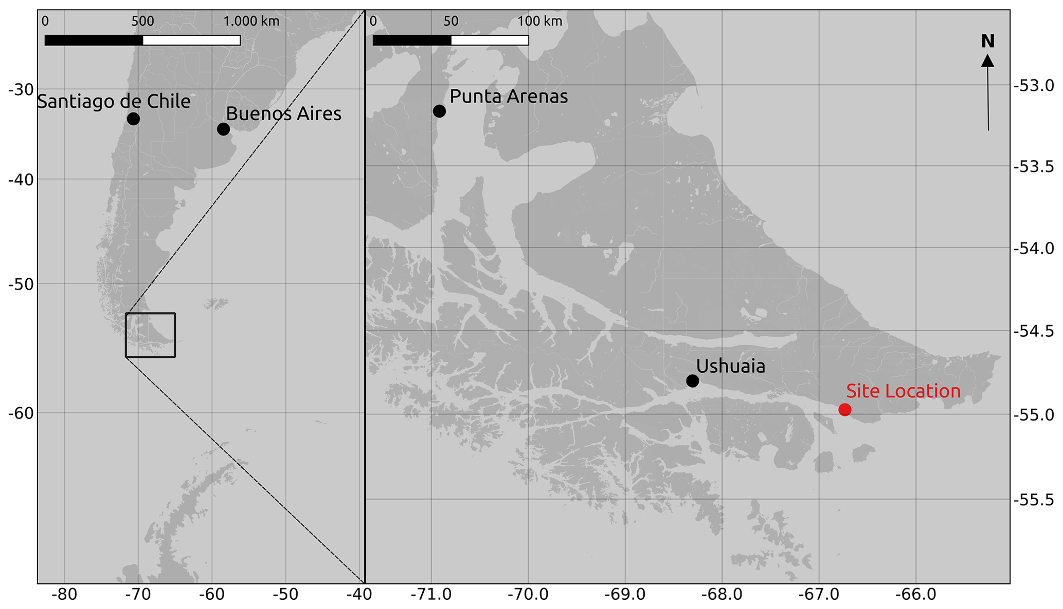
Figure 1Location of the study site, a cushion bog at the northern coast of the Beagle Channel, close to Punta Moat on Isla Grande de Tierra del Fuego, Argentina. (Map data: OpenStreetMap contributors 2020.)
2.2 Setup of warming experiment
In October 2014, we installed 20 plots, 10 of which were randomly assigned to receive warming treatment (treatment plots), where air and soil temperatures were passively increased by placing open-side chambers (OSCs) over the vegetation similarly to in the approach of Marion et al. (1997). The OSC, made of transparent polycarbonate in the shape of a semicircle open to the north, is 50 cm high and 1.30 m in diameter (Fig. 2). We measured the transmittance of a small section of polycarbonate in the visible region of the daylight spectrum with a spectrophotometer (UV-1203, Shimadzu Corporation, Japan), showing a high transmittance, ranging between 80 % and 85 %. Air temperature 1 cm above the canopy and soil temperature 10 cm below the surface were recorded hourly inside and outside the treatment plots in three replicates using HOBO U12 data loggers (Onset Computer Corporation, USA) between 1 January 2018 and 18 January 2019. The air probes were covered by shade caps to avoid direct sunlight while allowing free airflow around the probe. To evaluate if the treatment actually did affect temperatures, we calculated the differences between the treatment and the related control temperature measurements at each time step and calculated the mean difference. We then applied a randomization test (Edgington and Onghena, 2007) by randomly assigning each measurement to the treatment or control group and again calculating the mean difference. We repeated this step 10 000 times. Next, we compared the distribution of the 10 000 mean differences calculated with random treatment assignments to the actual mean difference between treatment and control using a one-sample t test. We regard the case when the actual mean is not likely (p<0.01) to come from the same distribution as the randomized mean differences as evidence for a significant treatment effect.
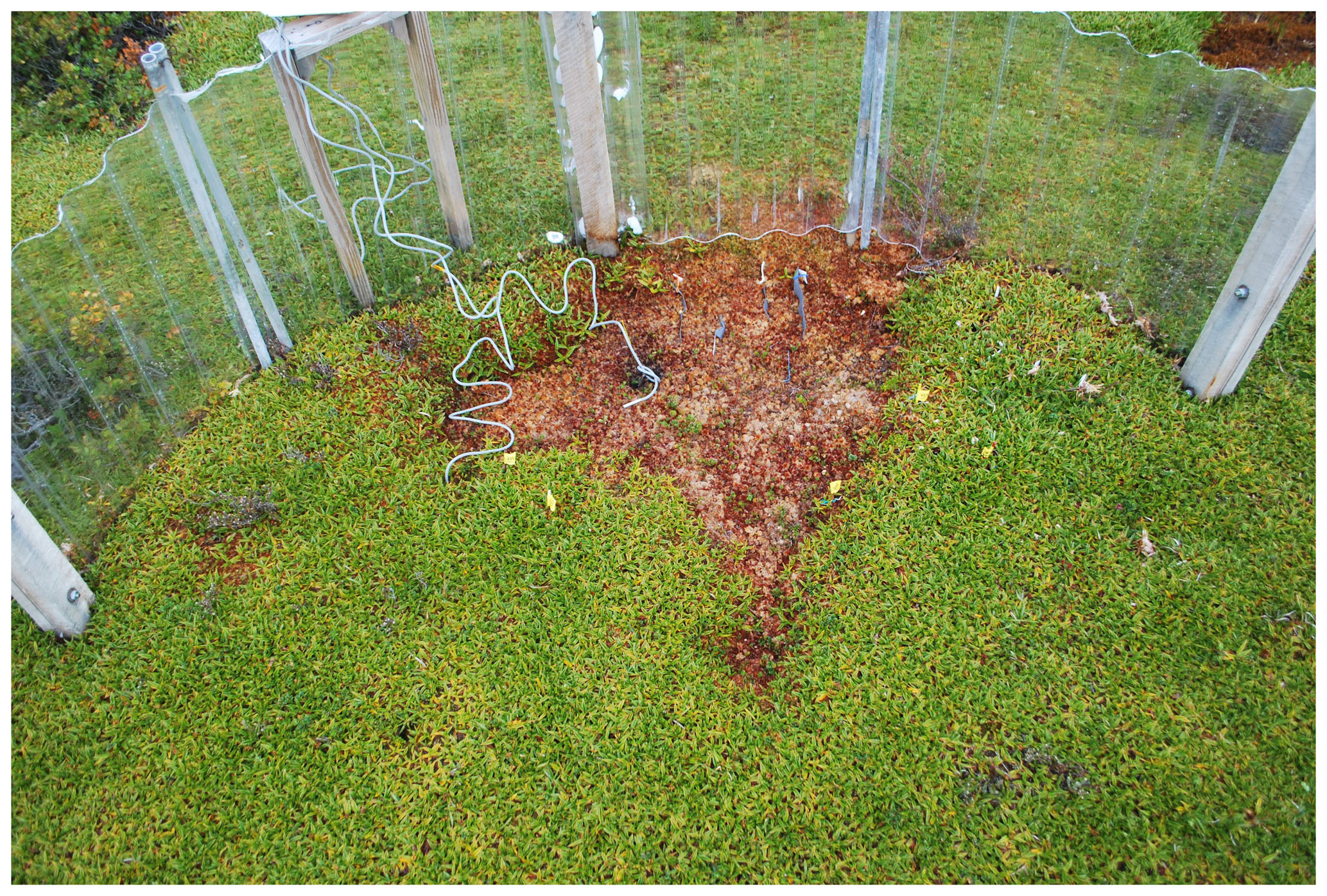
Figure 2Experimental setup. Open-side chamber (OSC), open to the north, installed in an Astelia pumila (light green color) cushion with a patch of Sphagnum magellanicum (reddish-brownish color).
2.3 Leaf properties
During two growing seasons (2015/16 and 2017/18), we conducted length measurements of Astelia pumila leaves and counted the number of total, green, and senescent leaves (see Tables S3–S5 in the Supplement). We selected 10 individuals per plot and labeled and measured the length (mm) of a young, fully expanded leaf at the beginning of the growing season using a digital caliper. We marked the measured leaves and determined the lengths of the same leaves at the middle and at the end of the growing season. From the treatment as well as the control plots, we recorded the lengths of 100 individual Astelia leaves for each group during the growing seasons of 2015/16 and 2017/18 at three (January, February, April 2016) and two (September 2017, March 2018) points in time, respectively. By subtracting the lengths of single leaves, which we tracked individually throughout two growing seasons, late in the season from the respective lengths at the beginning of the season, we estimated and compared average leaf growth at the treatment and control plots.
All leaves we sampled for lab analysis were put in plastic ziplock bags, transported to the lab, and stored in a refrigerator until the next day if they were not processed the same day. During 12 measurement days between 15 January and 4 March 2016 (see Table S2 in the Supplement), we sampled in total 86 sun-exposed, fully expanded leaves. We took pictures of the leaves which included a ruler so that we could estimate their area using the software ImageJ (Rueden et al., 2017). We divided the area estimates into two groups referring to midsummer and late summer and compared the respective treatment and control means using a Mann–Whitney U test of the SciPy Python library (Virtanen et al., 2020). Additionally, we determined the specific leaf area (SLA, cm2 g−1), leaf water content (LWC, %), and leaf dry mass content (LDMC, mg g−1). We estimated dry mass after drying the leaves in an oven at 65 ∘C for 72 h or to constant weight. We estimated LWC and LDMC following Pérez-Harguindeguy et al. (2016).
On six dates between January 2016 and September 2017, we sampled fully expanded Astelia leaves and extracted their photosynthetic pigments (chlorophyll and carotenoids; see Table S6 in the Supplement) using dimethyl sulfoxide solution (DMSO). We collected six leaves per plot and cut two 7.5 mm2 large disks from each leaf, resulting in 12 disks per plot. We macerated the disks in 5 mL of DMSO and heated them to 70 ∘C for 45 min (Barnes et al., 1992; Wellburn, 1994). We measured the absorbances at wavelengths of 665, 649, and 480 nm with a spectrophotometer (UV-1203, Shimadzu Corporation, Japan). We followed Wellburn (1994) to calculate chlorophyll a, chlorophyll b, and carotene contents.
To investigate the treatment effect on the number of plants per area, we counted the density of plant individuals in about 10 cm by 10 cm large areas within 10 treatment and 10 control plots (see Table S1 in the Supplement) in April 2016.
See Fig. S11 in the Supplement for an overview of the timing of our different sampling and measurement campaigns between 2014 and 2019.
2.4 Chamber soil–atmosphere CO2 flux measurements
We used a closed static chamber technique (Livingston and Hutchinson, 1995) to determine CO2 fluxes from the treatment and control plots between January 2018 to January 2019 (see Table A1). Chamber measurements were carried out using permanently installed PVC collars with a 0.4 m diameter and a height of 0.2 m, which were installed 0.15 m into the peat below the Astelia pumila lawns in both treatments in October 2014. We estimated the headspace, considering the distance from the vegetation to the border of the collar plus the height of the chamber above the collar. We identified and estimated plant species coverage within each collar (Table B2). We used a cylindrical, transparent chamber with a basal area of 0.12 m2 and a height of 0.4 m to conduct soil–atmosphere flux measurements of CO2 net ecosystem exchange (NEE). The chamber was internally equipped with a fan to ensure mixing of the headspace air, inlet and outlet ports to and from the infrared gas analyzer (IRGA; LI-840, Li-Cor Inc., USA), a sensor (HOBO S-LIA-M003, Onset, USA) to measure photosynthetically active radiation (PAR), and a temperature sensor (WatchDog 425, Spectrum Technologies, USA). CO2 and water vapor concentration data were logged at 3 s intervals and PAR was logged at 6 s intervals on a data logger (CR216, Campbell Scientific, Inc., USA). The chamber was connected by polyethylene tubing (2 mm inner diameter) to the IRGA. The gas analyzer was equipped with a pump transporting air from and to the chamber in a loop through the analyzer measurement cell. We avoided inducing a pressure pulse during chamber placement by equipping the chamber with a vent in its top cover. This opening was plugged immediately after the chamber was gently placed on a collar to conduct measurements. Collars were equipped with a water-filled rim to ensure a gas-tight seal between chamber and collar. Between the at least 3 min long measurements, the chamber was ventilated with ambient air until atmospheric background concentrations were measured inside the purged chamber. All measurements were performed under a broad range of irradiance, starting early in the morning and continuing until late afternoon to encompass diurnal variations in CO2 fluxes. At each collar, two or three consecutive measurements were performed with the transparent chamber, followed by dark measurements, which were achieved by completely covering the chamber with a 5 mm thick reflective polyester fabric with aluminum coating on the outside. During dark measurements, GPP was assumed to be zero, and the measured CO2 fluxes are therefore representative of ecosystem respiration, a combination of autotrophic and heterotrophic respiration.
2.5 CO2 flux calculation
We calculated CO2 fluxes using a routine (Eckhardt and Kutzbach, 2016) in MATLAB R2019a (The MathWorks, Inc., USA) that applies different regression models to describe the change in the chamber headspace CO2 concentration over time and conducts statistical analysis. This application also includes a graphical interface and allows for the calculation of a flux with respect to a manually selected period of a time during chamber closure. We visually inspected all measurements with this tool and removed periods with perturbed gas concentrations which often occurred shortly after chamber placement. To avoid a large impact of the greenhouse effect during closure time, we furthermore selected relatively short periods after the initial perturbations for flux calculation. As water vapor concentrations were measured simultaneously, we additionally selected periods during which water vapor concentrations did not go into saturation, potentially impacting plant activity and light transmittance of the chamber walls in the case of condensation. The time periods used for flux calculation were therefore generally much shorter than the chamber placement time. The median flux calculation period length was 48 s for the 81 treatment fluxes as well as for the 153 control fluxes (see Fig. A1 and Table A1). The comparably short time periods lead to close-to-linear concentration increases over time. We therefore used linear regression in all cases to calculate a gas flux from the estimated slope parameter () of the fitted line with Eq. (1).
where is the molar flux of carbon dioxide (), R is the ideal gas constant (8.3145 ), V is the chamber volume (m3), A the collar area (m2), pair is the air pressure (Pa), and Tair is air temperature (K). The air pressure (measured at the nearby eddy covariance station) and temperature (measured inside chamber), as well as chamber volume and collar area are assumed to be constant during a flux calculation period. Prior to function fitting, the measured CO2 concentrations were referenced to the initial water vapor concentration and recalculated to by applying Eq. (2).
where and are the concentrations of CO2 and water vapor as measured with the IRGA and is the initial water vapor concentration at the beginning of the flux calculation period. We propagated the standard error in the slope parameter and uncertainty estimates for the constants (air pressure, collar area, headspace volume) and variables (water vapor concentration and air temperature) in the flux calculation equation through Eq. (1) to calculate the absolute standard error in the flux. The median relative flux errors of about 15 % were similar for treatment and control fluxes (see Fig. A1).
2.6 CO2 flux modeling
We modeled the measured CO2 net ecosystem exchange (NEE) fluxes () from the treatment and control plots separately using a combination of two deterministic functions in a single bulk model as in Runkle et al. (2013). This model consists of a term modeling total ecosystem respiration (TER, ) as an exponential air temperature (T) relation and a light saturation function (rectangular hyperbola) of PAR to estimate photosynthesis (gross primary production GPP, ). As dark measurements (dark respiration Rd, ), where photosynthesis can be assumed to be inactive, were available in our data set (treatment, n=18; control, n=34), we first estimated the respiration parameters Q10 (dimensionless) and Rbase () in Eq. (3) (with the constants of reference temperature Tref=15 ∘C and γ=10 ∘C) from the dark flux measurements. Subsequently, we set these respiration parameter estimates as constants in the bulk model (Eq. 4) and optimized the GPP parameters of maximum photosynthesis Pmax () and initial quantum yield α (dimensionless) using all fluxes including the ones measured with transparent chambers (treatment, n=81; control, n=135). All parameter estimates were optimized using the SciPy Python library (Virtanen et al., 2020) by minimizing the squared model–data residuals. As the derived parameters can be interpreted as plant-specific, physiological properties due to our mechanistic modeling approach, we used them to characterize the treatment effect on plant properties.
Eventually, we drove the optimized NEE models with half-hourly PAR and T records from our meteorological station at the site to calculate net CO2 uptake of the treatment and control plots over the three main growing seasons (15 November to 15 March) 2016/17, 2017/18, and 2018/19. We calculated uncertainty estimates of each modeled GPP, TER, and NEE flux as 95 % confidence intervals based on Gaussian error propagation. The partial derivatives of Eq. (4) with respect to the parameters which we used in the course of error propagation are described in Holl et al. (2019). We simplified error propagation by ignoring the random errors in temperature and radiation measurements which we assume to be rather small compared to the uncertainty in the flux estimates. We calculated the uncertainty in the annual sums by taking the square root of the sum of squared uncertainties in the individual 30 min NEE sums.
3.1 Treatment effects on temperature
The open-side chamber treatment resulted in higher near-surface (1 cm above canopy) air temperatures at the treatment plots compared to the control plots. At the three replicate experiments which were equipped with temperature sensors, the mean air temperature difference over the measurement period of about 1 year was between 0.4 and 0.7 ∘C (see Fig. D5). These average annual differences are consistent over hourly raw data as well as over daily and weekly averaged temperature measurements (see Figs. D1 to D4). Soil temperatures at 10 cm depth were elevated in the same range only at two of the three replicate experiments. We suspect that sensor placement might have been suboptimal, and the temperature probe was not installed as deep as at the other plots. Annual means of daily and weekly averaged soil temperature differences were between 0.2 and 0.3 ∘C and 0.0 ∘C at the third plot.
As another way to characterize the temperature differences caused by the treatment, we calculated average diurnal cycles for single months and seasons (see Figs. S1 to S8 in the Supplement). We applied Mann–Whitney U tests to compare the distribution means at each hour of the day. We found significant (p<0.1) mean air temperature differences between control and treatment mostly at midday, between 13:00 and 15:00 LT, coinciding with the solar radiation maximum. Midday maximum differences ranged between 1.2 and 3.0 ∘C in spring and summer and between 1.0 and 2.0 ∘C in autumn and winter. At other times of the day, significant air temperature differences were only found at one of the three plots during autumn and winter. The timing of significant seasonally averaged soil temperature (10 cm below the surface) differences at single hours of the day is less consistent over the replicate plots (compared to the timing of maximum air temperature differences). In summer and at two of the three plots, we found significant differences between midnight and the early morning. Maximum soil temperature summer differences occurred between 03:00 and 05:00 at all three replicates. In winter, the comparably smaller temperature differences had significantly different means at each hour of the day, while the diurnal course and the timing (11:00, 18:00, 22:00) of the maximum difference appears to be inconsistent over the three replicate plots. In spring and summer, maximum soil temperature differences lay in between −0.2 and 0.4 ∘C, meaning that at one plot, the treatment apparently led to a soil temperature decrease. The same was the case in autumn and winter when maximum soil temperature differences ranged between −0.2 and 0.6 ∘C.
Results of the randomization test (see Fig. D5) show that the mean hourly temperature differences we measured between treatment and control plots were not only caused by random noise. The randomly generated mean temperature differences are centered around zero, and the probability of the actual mean difference to come from this generated distribution is very low (one-sample t test, p<0.001). We therefore conclude that the OSC treatment did increase surface as well as soil temperatures in the treatment plots significantly. In the case of the soil temperatures the increases were, however, smaller and not consistent over the three replicates.
3.2 Treatment effects on leaf properties
In 2016, the average treatment leaf was significantly (Mann–Whitney U test, p<0.01) shorter in midsummer (January, February) and at the end of the growing season (April) compared to the control leaves. Within each treatment, leaf lengths were significantly (Kruskal–Wallis test, p<0.01) different from each other in January, February, and April 2016, indicating leaf growth. In contrast, at the beginning of the growing season (September 2017) of 2017/18, treatment leaves tended to be longer than control leaves on average (Mann–Whitney U test, p<0.1). In the late growing season (March 2018) of 2017/18, we could not find a significant difference (p=0.3) between control and treatment leaf length means (see Fig. 3).
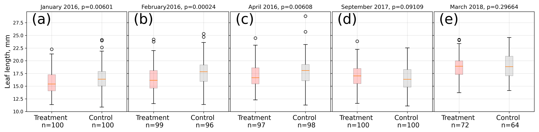
Figure 3Comparison of A. pumila leaf lengths from treatment and control plots throughout the growing seasons 2015/16 (a–c) and 2017/18 (d, e). Mann–Whitney U tests indicate highly significant (p<0.01) differences between treatment and control leaf lengths in 2016. In September 2017, leaf lengths are only different at a lower significance level (p<0.1). In March 2018, leaf lengths did not differ between treatment and control plots.
Table 1Estimated average growth rate (µm d−1) of individual Astelia pumila leaves at the treatment and control plots in two seasons. Length measurements were taken on 13 January and 29 April 2016, 25 September 2017, and 7 March 2018. Differences were divided by the number of days between observations to calculate growth rate.
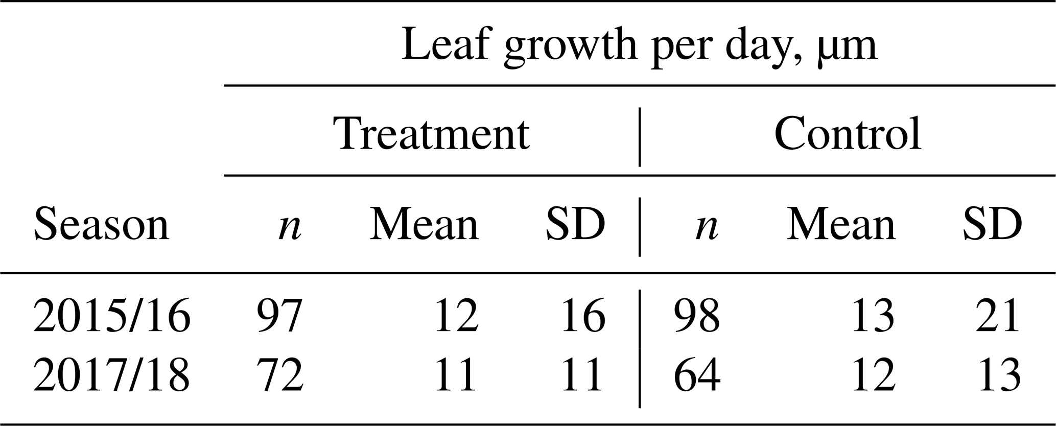
Average leaf growth (see Fig. B1) was not significantly different (Mann–Whitney U test, p>0.2) between treatment and control plants either in 2016 (13 January to 29 April 2016, 1.34 mm±2.21 mm (control) and 1.28 mm±1.76 mm (treatment)) or in 2017/18 (25 September 2017 to 7 March 2018, 1.99 mm±2.20 mm (control) and 1.77 mm±1.83 mm (treatment)). Again indicating plant development, one-sample t tests and Wilcoxon signed rank tests show that the average growth is significantly different (p<0.0001) from zero for both growing seasons and at the treatment and control plots. We calculated leaf growth per day by normalizing the length increases with the observation period length for the respective season (see Table 1). This average leaf growth rate is with about 12 µm d−1 virtually constant for both treatments and in both seasons.
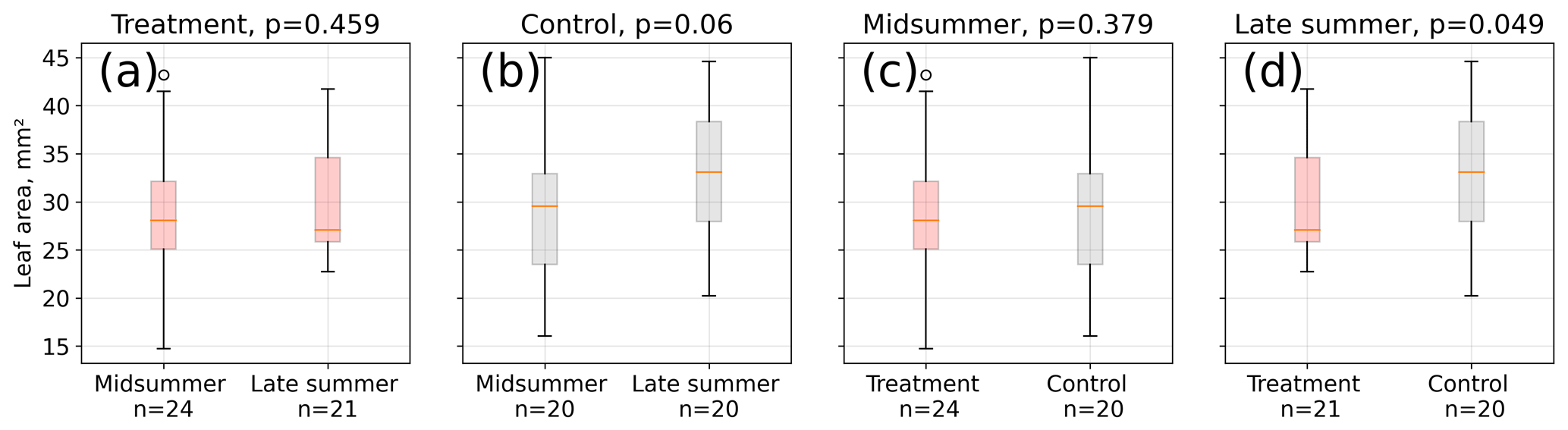
Figure 4Leaf area measurements from 12 measurement days between 15 January and 4 March 2016. We divided the area estimates into two groups referring to midsummer and late summer (see Table S2) and compared the respective treatment and control means using a Mann–Whitney U test. Average leaf area was not different between midsummer and late summer at the treatment plots (a), whereas control plot leaves (b) were on average longer in late summer than in midsummer, although at a low significance level (p<0.1). Treatment and control plant average leaf area differed significantly in late summer (d, p<0.05) but not in midsummer (c, p=0.4).
Leaf area differences were only significant (p<0.05) in late summer indicating a larger mean leaf area at the control plots (see Fig. 4). Leaf area means within the treatment group were not significantly different between midsummer and late summer. In contrast, the leaf area of the control plants was significantly (p<0.1) larger in late summer compared to in midsummer. It has to be noted that the number of samples for these comparisons was limited; test results may therefore not be robust.
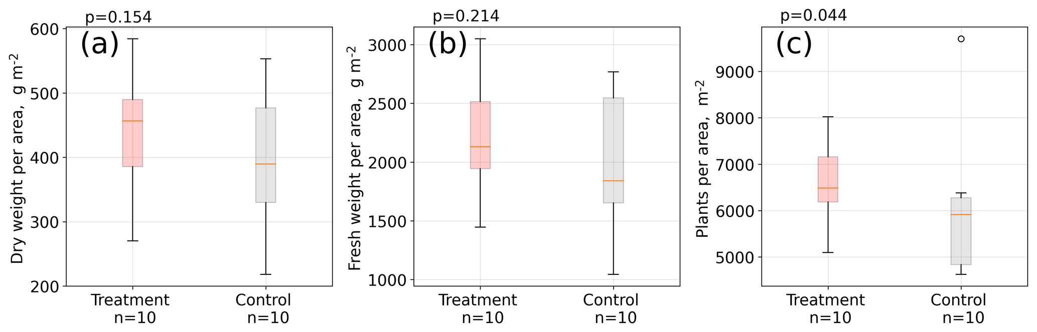
Figure 5Aboveground A. pumila biomass. Dry weight (a) and fresh weight (b) per area and individual plants per area (c). Measurements were taken in April 2016 in about 10 cm by 10 cm large sampling rectangles within the control and treatment plots (see Table S1). About 1.5 years after the installation of the open-side chambers in October 2014, a significantly (Mann–Whitney U test, p<0.05) denser plant cover developed at the treatment plots compared to the control plots (c).
Results from our areal plant density estimation (see Table S1) suggest that areal plant density is significantly (Mann–Whitney U test, p<0.05) higher at the treatment plots compared to the control plots, whereas mean aboveground biomass per area is larger at the treatment plots but not significantly different (p=0.2) from the control plots (see Fig. 5). Simultaneously to the leaf length measurements in two growing seasons, we counted the total number of leaves per plant in January 2016 for 100 control and 100 treatment plants. The total number of leaves was seven and equal for both groups (see Table S3 in the Supplement). We did not detect differences in leaf water content, leaf dry mass, and specific leaf area between treatment and control plants (see Table S2).
We did not find significant differences in absolute leaf pigment contents between treatment and control plants on any of the measurement days (see Table S6). However, when considering the increase in pigments from the mid-growing season to its end, we found that on average control leaves increased chlorophyll a by a significantly (Mann–Whitney U test, p<0.05) larger amount between February and May 2016 than treatment leaves (see Fig. 6).
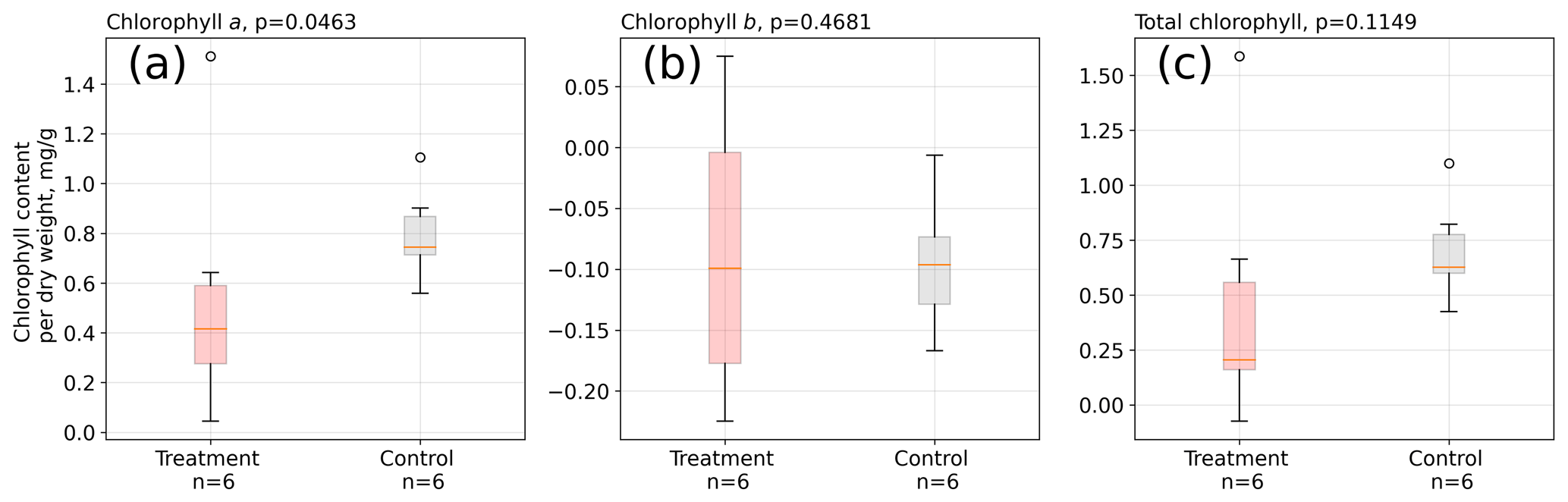
Figure 6Change in chlorophyll contents from February to May 2016 in A. pumila leaves from treatment and control plots. During this growing season, control plants appear to have increased their chlorophyll a content (a) to a significantly (p<0.05) greater extent than treatment leaves. Differences in the contents of chlorophyll b (b) and total chlorophyll (c) did not change significantly. The sample size is, however, not large enough to firmly make these assertions.
Accordingly, treatment plants had the same number of leaves, which were, however, shorter (5 %) and with a smaller (10 %) surface area at the end of the season than control plants, whereas the number of plants per area increased (10 %) at the treatment plots, so leaf biomass per area and specific leaf area were the same in both groups.
3.3 Treatment effects on CO2 fluxes
We estimated bulk model parameters separately for control and treatment fluxes. With high coefficients of determination and with respect to the range of measured fluxes' relatively low root mean square errors (RMSEs), the model quality appears to be sufficient to yield meaningful parameters in all four cases (see Figs. 7 and 8). Distinctions between treatment and control are most pronounced with respect to the parameter expressing the temperature sensitivity of respiration (Q10) and the parameter denoting the theoretical maximum photosynthesis at an infinite photon supply (Pmax). From the dark measurements (Fig. 7), we estimated a nearly 80 % larger Q10 at the treatment plots (control, 2.8; treatment, 5.0). At the same time, Pmax, as estimated from the bulk model fit to chamber measurements (Fig. 8), was more than 40 % lower at the treatment plots (control, 15.9 ; treatment, 9.2 ). We found less pronounced differences for base respiration Rbase at 15 ∘C, which was elevated by 16 % at the treatment plots (control, 4.21 ; treatment, 4.89 ), and for the initial quantum yield α, which was 23 % larger at the treatment plots (control, 0.031; treatment, 0.038). A comparison (see Fig. C1) with bulk model parameter time series, which Holl et al. (2019) estimated from eddy covariance data at the same site for 2 years, reveals that our chamber-derived parameters are representative of the main growing season (15 November to 15 March). During this period, the control plot parameters from this study are in line with eddy covariance ecosystem-scale estimates. Chamber flux measurements were biased towards the mid-growing season (see Table A1 and Fig. C1b) where chamber-derived parameter estimates also overlap with eddy covariance parameter time series.
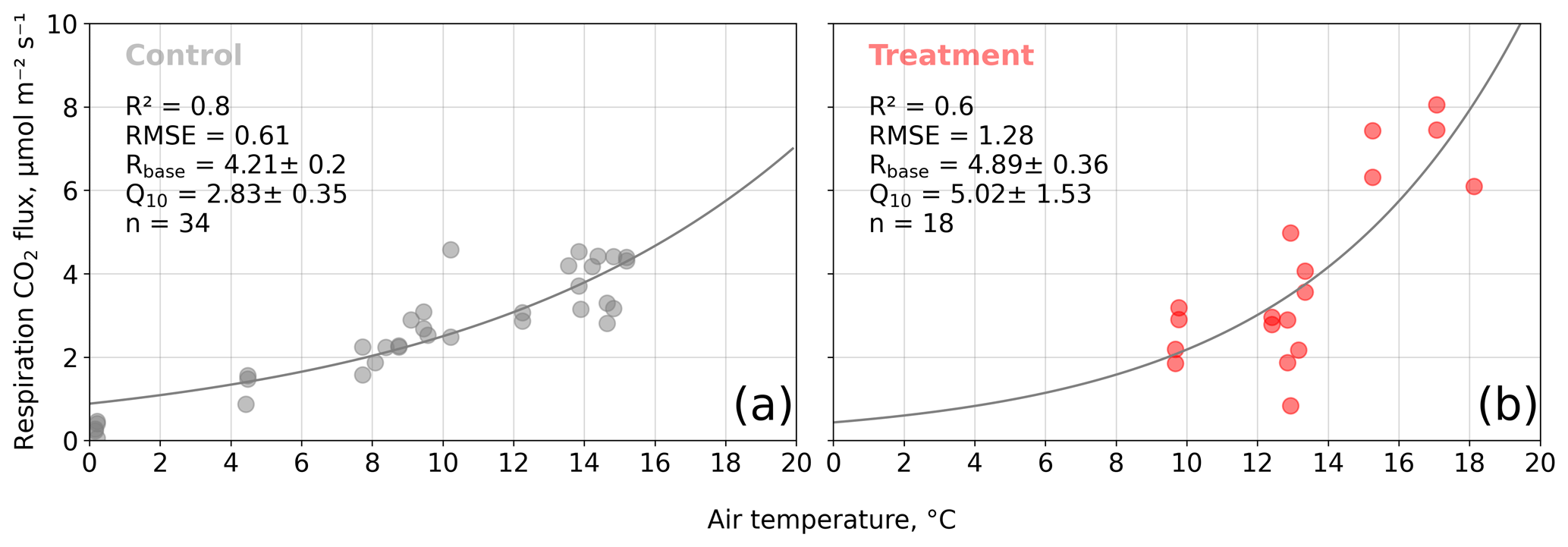
Figure 7Dark respiration measurements acquired with opaque chambers at the control (a) and treatment (b) plots versus air temperature. We fitted an exponential function of air temperature (see Eq. 7) to the measured carbon dioxide (CO2) fluxes to estimate the ecosystem respiration parameters base respiration Rbase () and temperature sensitivity Q10 (dimensionless). Coefficients of determination (R2) and root mean square errors (RMSEs) are given.
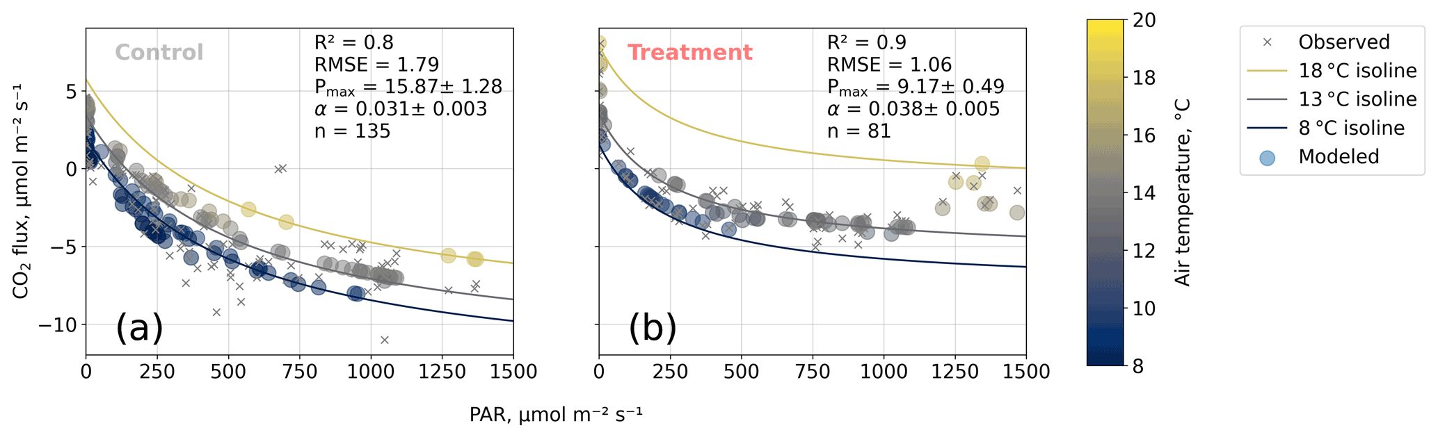
Figure 8Net carbon dioxide (CO2) flux versus photosynthetically active radiation PAR (). We modeled observed net CO2 fluxes from chamber measurements as a function of PAR and air temperature with our bulk model (see Eq. 4). Two of the four bulk model parameters (Q10 and Rbase) were determined based on dark respiration measurements (see Fig. 7) and set as constants so that the bulk model was used to optimize the parameters' maximum photosynthesis Pmax () and initial quantum yield α (dimensionless). Coefficients of determination (R2) and root mean square errors (RMSEs, ) are given.
The fact that, at the treatment plots, the bulk NEE partitioning model is able to explain the comparably small CO2 uptake in the high radiation range (PAR>1200 ; see Fig. 8b) further increases our confidence in the stepwise bulk model approach. Moreover, this behavior highlights distinctive treatment effects on plant and soil traits: photosynthesis at the treated plots could not profit as much from higher radiation input as at the control plots while ecosystem respiration was promoted more by simultaneously increased temperatures, so net CO2 uptake in high radiation and high temperature conditions is severely attenuated at the treatment plots. This temperature-dependent respiration increase can outweigh photosynthetic CO2 uptake at high temperatures (see 18 ∘C isoline in Fig. 8b) across the whole radiation range.
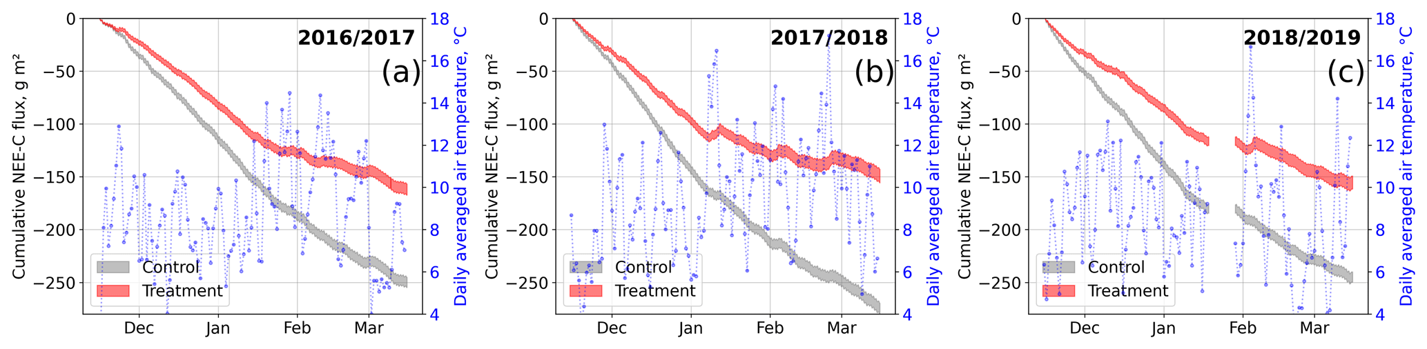
Figure 9Modeled cumulative net ecosystem exchange (NEE) fluxes of CO2 at the control and treatment sites, expressed as carbon (C) fluxes for three seasons. The cumulation period represents the main growing season from 15 November to 15 March. We used the previously determined bulk model parameters (see Figs. 7 and 4) and observations of air temperature and photosynthetically active radiation to drive the models. Gaps in these time series in 2019 led to a gap in the cumulative curve in (c). Areas represent the upper and lower bound of the model uncertainty.
To investigate the treatment effect on growing-season NEE sums, we drove the bulk models with half-hourly temperature and radiation data measured at our site. We used data from the three main growing seasons 2016/17, 2017/18, and 2018/19 between 15 November and 15 March. Due to a gap in meteorological data in 2019, we report only cumulative fluxes from the first two seasons here; data for 2018/19 are plotted in Fig. 9. The results document drastic differences in cumulative net CO2 uptake between the control and treatment plots which are consistent over both the main growing seasons considered. The control plots sequestered between 55 % and 85 % more atmospheric CO2−C (2016/17, g m−2; 2017/18, g m−2) than the treatment plots (2016/17, g m−2; 2017/18, g m−2). According to the data-based models, during 3 weeks in 2018 (7 to 12 January, 1 to 7, and 20 to 26 February), the treatment plots even turned from sinks into sources of atmospheric CO2 as indicated by the upward-sloping cumulative curve during these especially warm periods.
Our results show that the OSC treatment significantly increased air temperatures at the respective plots in the cushion bog of this study. As this method is inexpensive, causes limited soil disturbance, and requires little maintenance and no power supply, it is especially suitable for remote sites and thus has commonly been applied in ecosystem warming experiments (e.g., Aronson and McNulty, 2009), including at sites with low vegetation like peatlands (Malhotra et al., 2020; Munir et al., 2015) or steppes (Liancourt et al., 2012; Sharkhuu et al., 2013). The temperature increases achieved by our OSC treatment are consistent with other passive warming experiments at high latitudes (Rustad et al., 2001; Zaller et al., 2009; Bokhorst et al., 2011). Compared to these studies, the increment of near-surface (1 cm above canopy) air temperature in our study (0.4 to 0.7 ∘C) was in the same range (Bokhorst et al., 2007; Prather et al., 2019) or smaller with respect to the results of Day et al. (2008) from Antarctica (1.3 to 2.3 ∘C) or the warming of 1.0 to 3.6 ∘C achieved in a tundra experiment (Biasi et al., 2008; Walker et al., 2006). Our OSC treatment led to significantly elevated air temperatures mainly during the daytime as also observed in previous studies (Marion et al., 1997; Bokhorst et al., 2007) and to increased air temperatures during all four seasons. As opposed to air temperatures, our OSC treatment did not affect soil temperatures consistently over the replicate plots. The increases in soil temperatures were generally lower compared to the air temperature increments. On the other hand, as shown by the results of the randomization test (see Fig. D5), soil temperature differences between treatment and control plots are unlikely to be caused by random processes only, indicating a, however inconsistent, treatment effect.
Apart from the desired temperature increase by reduced radiative energy loss, an OSC method can have secondary effects (Aronson and McNulty, 2009; Marion et al., 1997) like shading, altered micro-local wind patterns, and attenuated turbulence or reduced radiation input. We are confident that in our experimental study, we were able to minimize these secondary effects by installing the semicircular plastic wall with its open half facing northwards. Due to the position of our site in the Southern Hemisphere, incoming radiation was only attenuated early in the morning and late in the afternoon, while the treatment plots received direct radiation throughout most of the day. Moreover, we determined the light transmissivity of the wall material and found it to be between 80 % and 85 %. As winds most frequently came from north-northwestern directions, wind shelter effects caused by the OSCs were limited. At the fewer times when winds came from southern directions, sheltering by the OSC walls was most intense. However, the thereby attenuated turbulent energy transport did not consistently result in intensified warming across the replicate plots as shown in Fig. S9 in the Supplement. At Plot 24, warming was slightly (about 0.1 ∘C) more intense during west-southwestern winds. At Plot 22, where warming was least effective overall, attenuated turbulent energy transport could explain the observed intensified warming during winds from the sheltered south-southwestern directions. Additionally, phases of north-northwestern wind directions at the same time were phases of relatively warm air temperatures (at 2 m, measured at eddy covariance station; see Fig. S10 in the Supplement), so at Plot 25, warming was most intense during north-northwestern wind directions, when sheltering effects were most limited. A secondary effect we could not counteract lies in the fact that the detected temperature differences were not consistent over the course of a day. Therefore, a small temperature increment at certain times of day and a larger difference at other times of day exposes the treatment plots not only to larger average temperatures but also to a larger temperature range.
Between 1.5 and 3.5 years after the OSC treatment had been installed, we observed distinctions between the morphological features of the A. pumila plants in the control and treatment plots. However, leaf growth (i.e., length increase) did not differ significantly between treatment and control plants. In general, the growth rates we found are low but similar to values of other herbaceous vascular plants at comparable latitudes reported in the literature (Day et al., 2001; Rousseaux et al., 2001; Searles et al., 2002; Robson et al., 2003).
Concurrently to the morphological alterations, we found that in treated plants certain physiological properties were modified. In particular, we observed a tendency for the treated plants to increase their chlorophyll a content less throughout the growing season (see Fig. 6) than control plants. At the treatment plots, a degradation in the efficiency of GPP, especially at high light levels, is documented by our bulk model parameter estimates showing reduced maximum photosynthesis and elevated initial quantum yield. Conversely, ecosystem respiration was enhanced considerably at the treatment plots. We could validate the bulk model parameter estimates we derived from plot-scale chamber measurements at the control plots with ecosystem-scale eddy covariance measurements from the same site. Additionally, the eddy covariance parameter estimates are given as time series and thus enable an assessment of a period the chamber-derived parameters are representative of. We found that the stage of plant development during the main growing season (15 November to 15 March) is best represented by the parameters reported in this study.
A large discrepancy exists between the temperature sensitivity parameters Q10 at the plot and ecosystem scale. The Q10 estimate from eddy covariance is in line with values from most global ecosystems (1.4±0.1; Mahecha et al., 2010; Zhang et al., 2017), but, in contrast to plot-scale measurements, this signal is representative of a mixture of surface types typical of cushion bogs including pools or moss-dominated patches. Especially due to the exclusion of pools, an elevated temperature sensitivity can therefore be expected on the plot scale. However, a methodological bias could exist due to transient increases in leaf respiration when previously light-exposed plants are suddenly darkened as reviewed by Heskel et al. (2013). If such a bias exists, it would affect our stepwise bulk model approach (as our assumption that Rd is equal to TER would not hold) and therefore could alternatively explain the Q10 discrepancy because, in its first step, dark measurements are used to estimate the respiration parameters Q10 and Rbase (see Eq. 3). On the other hand, we might have avoided disturbances caused by transient plant responses by excluding initially perturbed gas concentrations prior to flux calculation.
We tested if with a full four-parameter bulk model, which should largely remove the abovementioned bias as it does not rely on dark measurements, respiration parameter estimates would differ from those derived with the stepwise approach (see Table C1). Full bulk model Q10 estimates of the treatment plots are still much higher (3.65±0.64) than the eddy covariance estimate but lower than the result when only using dark-chamber measurements (5.02±1.53) to determine Q10 and Rbase. However, the impact of choosing different sets of respiration parameters on the cumulative growing-season TER sums for the three considered growing seasons is somewhat counterintuitive. Table C1 shows the respiration parameters we derived from the alternative modeling approaches and the relative differences in the cumulative growing-season TER sums calculated with these alternative models. In all six cases (three seasons, two treatments), the full four-parameter bulk model TER estimate is between 10 % and 20 % larger than the stepwise estimate despite the larger Q10 estimates from the stepwise approach. The reason for the larger TER sum from the model in which both parameters are smaller is that air temperature during the summation period often was below the reference temperature of 15 ∘C (see Eq. 3). We therefore assume that when optimizing many model parameters at the same time, equifinality issues might be more important sources of uncertainty than transient respiration increases in suddenly darkened plants. Moreover, the stepwise bulk model gives the more conservative TER estimate, making our conclusion of increased respiration in the treatment plots less likely to be the result of an overestimation due to a methodological bias.
As discussed above, we are confident that increased respiration at the treatment plots can be asserted. Due to the limited impact of the warming treatment on soil temperatures, we speculate that this increased total respiration could largely be attributed to enhanced autotrophic respiration. Commonly (e.g., Chapin et al., 2011), upward-bending PAR–NEE curves at high light levels (Fig. 8b) can be explained by photooxidation, i.e., the (adverse) physical effect of high-energy photons on plant tissue. In a warming experiment in a sub-Arctic (68∘ N) heath community, Bokhorst et al. (2010) found that warming caused stress and enhanced lipid peroxidation resulting in cell and tissue damage in treatment plants. In our study, the A. pumila plants under warming treatment could have been more prone to photooxidation due to warming-induced stress.
A possible explanation for the simultaneous increase in respiration along with a diminished efficiency of photosynthesis has been outlined by Brooks and Farquhar (1985) and by Dusenge et al. (2019). The authors found that photorespiration can be enhanced at elevated temperatures due to the decreasing ability of the enzyme RuBisCO to distinguish between CO2 and molecular oxygen (O2) with increasing temperatures. The – for the purpose of photosynthetic efficiency preferable – carboxylation reaction (CO2 fixation) can thereby be hampered while the oxygenation reaction (CO2 release) is intensified. The result of such a mechanism would match our observations of the elevated temperature sensitivity of respiration and the diminished GPP at the treatment plots. On the other hand, the temperature difference archived in our treatment experiment might have been too small to cause the observed differences by the above-described dependency of RuBisCO characteristics on temperature. The GPP differences between treatment and control plots in this study are additionally connected to the observed changes in leaf area and leaf chlorophyll a content in the course of the growing season which were both larger at the control plots. The differences in the latter plant traits might have driven GPP variability primarily or in conjunction with the temperature dependence of RuBisCO properties. An alternative or additional explanation for the increased respiration at the treatment plots might be connected to A. pumila root dynamics which we did not observe in this study. Cushion plants develop a high belowground-to-aboveground biomass ratio (Fritz et al., 2011) and a relatively large, dense root and rhizome system (Kleinebecker et al., 2008). Root growth might have been intensified by the warming treatment, as observed in the study of Malhotra et al. (2020), and could have led to enhanced respiration.
In our study, warming was paralleled by alterations of morphological and physiological cushion plant properties. Treated A. pumila plants formed denser cushions consisting of smaller individual plants; their photosynthetic capacity was hampered while respiration was intensified leading to a drastically diminished growing-season CO2−C net sink at warmed A. pumila cushions. Other warming studies found similar as well as contrary effects of experimental warming on plant properties. In general, vegetation responses to warming are highly species-specific as noted by Prather et al. (2019). Studying the impact of warming on maritime Antarctic plant communities, Bokhorst et al. (2007) found that open plant communities (grasses and lichens) were more negatively affected by warming than densely growing plants like mosses and dwarf shrubs. Similarly, Walker et al. (2006) report that woody plants benefited from warming at 11 sites across the tundra biome. Contrary to Bokhorst et al. (2007), Walker et al. (2006) show that moss and lichen cover decreased as a result of warming. As also indicated at our site by a longer average treatment leaf length at the onset of the growing season (see Fig. 3d), Livensperger et al. (2016) report accelerated plant development at passively warmed plots in the initial growing season from an Eriophorum-dominated tussock tundra site on the North Slope of Alaska. While the tussock community development was accelerated in spring, overall growing-season plant growth did not increase, matching our observations at the cushion bog. Furthermore, Bokhorst et al. (2010) identified spring-like plant development in winter in warmed plots at a sub-Arctic (68∘ N) heathland as the major driver of warming-induced tissue damage which manifests as lipid peroxidation and impacts metabolic efficiency. In general, cold and wet ecosystems appear to be more sensitive to warming than drier ecosystems (Peñuelas et al., 2004). At a microform level, a similar observation was made by Munir et al. (2015) with respect to growing-season CO2−C net uptake in a Sphagnum-dominated bog in Canada (55∘ N). The authors found that at drier hummocks net CO2 uptake was elevated by warming, whereas at wetter hollow sites, more CO2 was emitted. Likewise, Hopple et al. (2020) report an increase in dark respiration with temperature based on a warming experiment in a Sphagnum-dominated, treed, low-shrub bog in Minnesota (47∘ N).
We conducted a warming experiment in a Southern Hemisphere cushion bog to investigate responses of the cushion-forming plant Astelia pumila to elevated temperatures as they are projected to occur in the Southern Hemisphere in a future climate. At warmed plots, A. pumila grew in denser cushions and had shorter leaves while aboveground biomass per area was unchanged. Furthermore, A. pumila physiology was altered so that at warmed plots, photosynthesis was less efficient while respiration was intensified. We propose an increase in photorespiration as a response to warming as one likely underlying mechanism since it could explain the diminished gross primary production and enhanced respiration simultaneously. Apart from alterations of the photosynthetic apparatus, differences in leaf morphology and chlorophyll contents between treatment and control plants most likely additionally, or even decisively, contributed to the observed GPP variability. Respiration variability could additionally have been impacted by changes in root respiration and stress-induced enhanced photooxidation.
Over the main growing season of 2 exemplary years, warmed A. pumila cushions cumulatively took up 55 % and 85 % less CO2−C than the cushions of unaltered control plots. This change in net C uptake is considerable, especially when comparing the amount of artificial warming achieved in our experiment (annual average between 0.4 and 0.7 ∘C at the 3 of the 10 replicates which were equipped with temperature sensors) with temperature projections for the region from the Coupled Model Intercomparison Project Phase 6 (CMIP6). Estimates for contrasting shared socioeconomic pathways (SSPs) show increases in mean annual 2 m air temperature of 1 ∘C (SSP1-2.6) and 2 ∘C (SSP5-8.5) from 2014 to 2100 (Wieners et al., 2019a, b). In conjunction with our findings, a considerable weakening of the long-term C sink strength of austral cushion bogs in a future climate seems likely. However, the temporal cover of flux measurements in our study was biased towards the growing season, and more data from the shoulder seasons and winter, when temperatures are lower but photosynthesis of the evergreen A. pumila is ongoing, would be desirable and should be collected in future studies.
Table A1Number of chamber CO2 flux measurements we conducted between January 2018 and January 2019 at the treatment and control plots of our site.
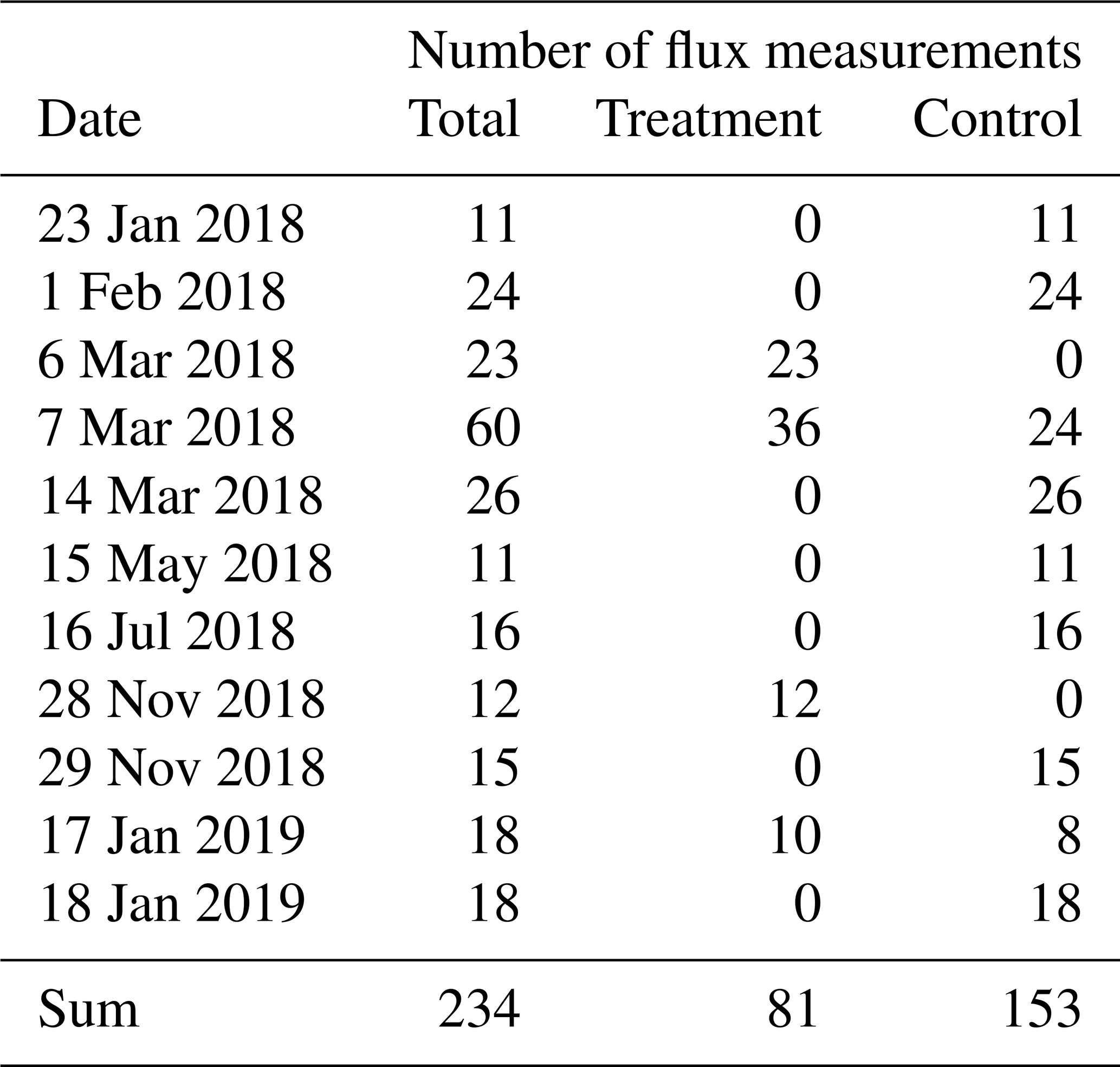
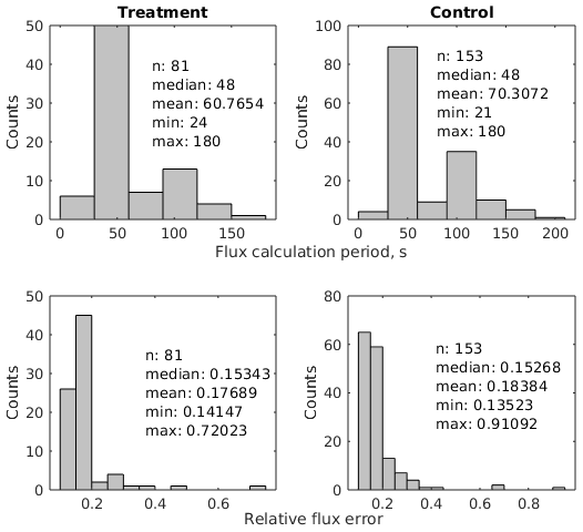
Figure A1Flux calculation statistics. Of the 3 min chamber closure time, a median period of 48 s was selected for flux calculation. Flux uncertainties mostly amounted to between 10 % and 20 % of the respective flux.
Table B1Comparison of the meteorological conditions at our study site during three consecutive seasons. Growing degree days (GDDs) are defined as the sum of all positive differences between daily average temperatures and reference temperatures of 5 ∘C (GDD5) and 10 ∘C (GDD10). The warmest year on average was 2016/17, and warm days (largest GDD5) occurred most consistently during this year. Additionally, this year's summer was very rainy. The year 2017/18 had by far the most very warm days (largest GDD10), especially in summer, and was also the driest year.
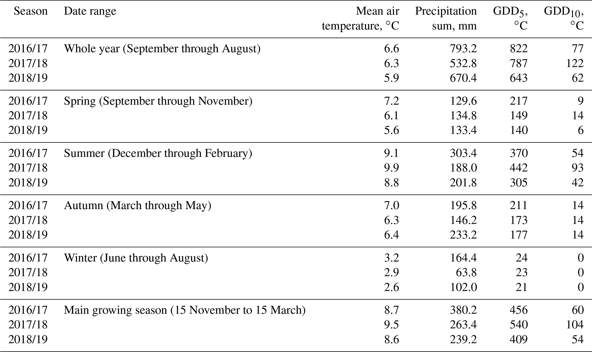
Table B2Estimated plant coverage at three treatment plots and three control plots where gas flux measurements were performed.
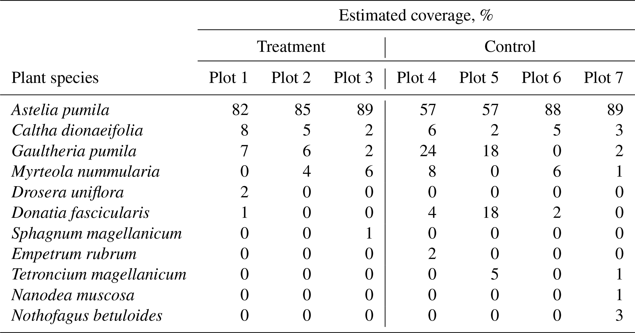
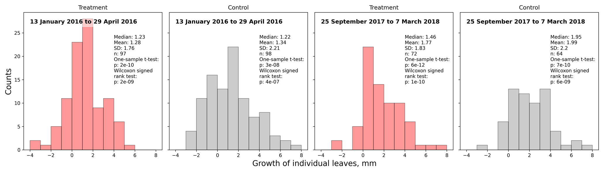
Figure B1Distribution of leaf growth estimates for Astelia pumila at the control and treatment plots. Growth estimates are calculated as differences in length measurements of leaves which we individually tracked throughout the season. We attribute the occurrence of negative growth values to random measurement uncertainty in the length measurements with a digital caliper. One-sample t tests and Wilcoxon signed rank tests from the SciPy Python library were used to check if the average growth values were significantly different from zero; i.e., growth took place.
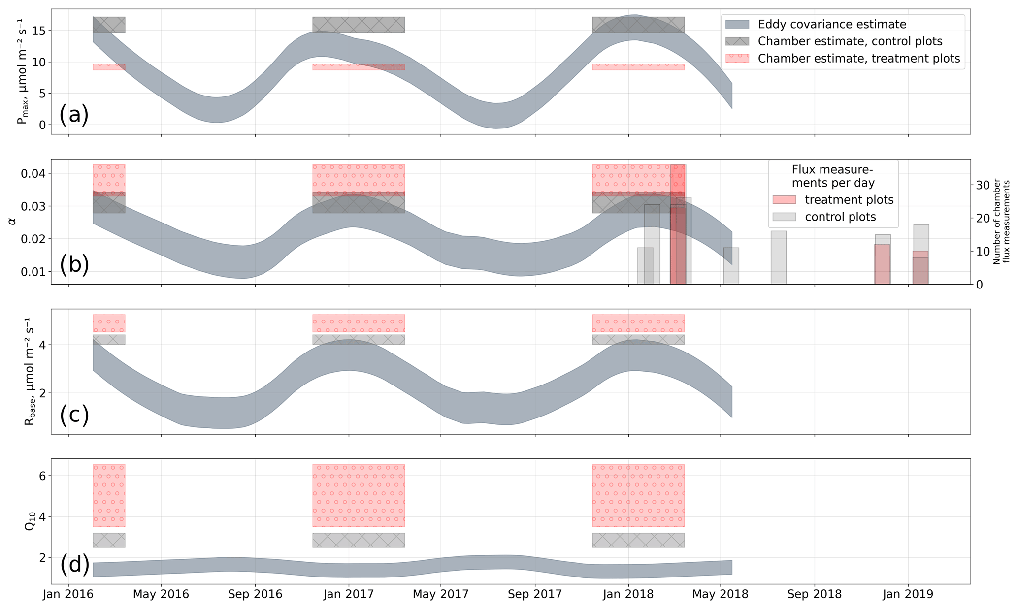
Figure C1Comparison of bulk model (see Eq. 4) parameters from this study with parameter time series derived from eddy covariance measurements by Holl et al. (2019) for the same site. (a) Photosynthetically active radiation Pmax; (b) initial quantum yield α (dimensionless); (c) base respiration Rbase; (d) temperature sensitivity of respiration Q10. The comparison allows for an estimation of a period within the seasonal course that the chamber-derived parameters are representative of. We found that the parameter estimates from this study best represent conditions during the main growing season towards which our chamber measurements are biased (see secondary y axis in b).
Table C1Respiration parameters base respiration Rbase () and temperature sensitivity Q10 derived from optimizing the full (four-parameter) bulk model (Eq. 4) compared with the estimation from dark measurements (Eq. 3) within our stepwise bulk-modeling approach. Additionally, the impact of choosing differently derived parameter sets on the cumulative total ecosystem respiration sums ∑TERfull and ∑TERstep over the main growing seasons (15 November to 15 March) of 3 exemplary years for which air temperature records exist for our site are shown. Full bulk model TER sums for the treatment and control plots are between 10 % and 20 % larger than stepwise bulk model TER sums which we used to calculate carbon dioxide net ecosystem exchange sums (see Fig. 9) in this study.
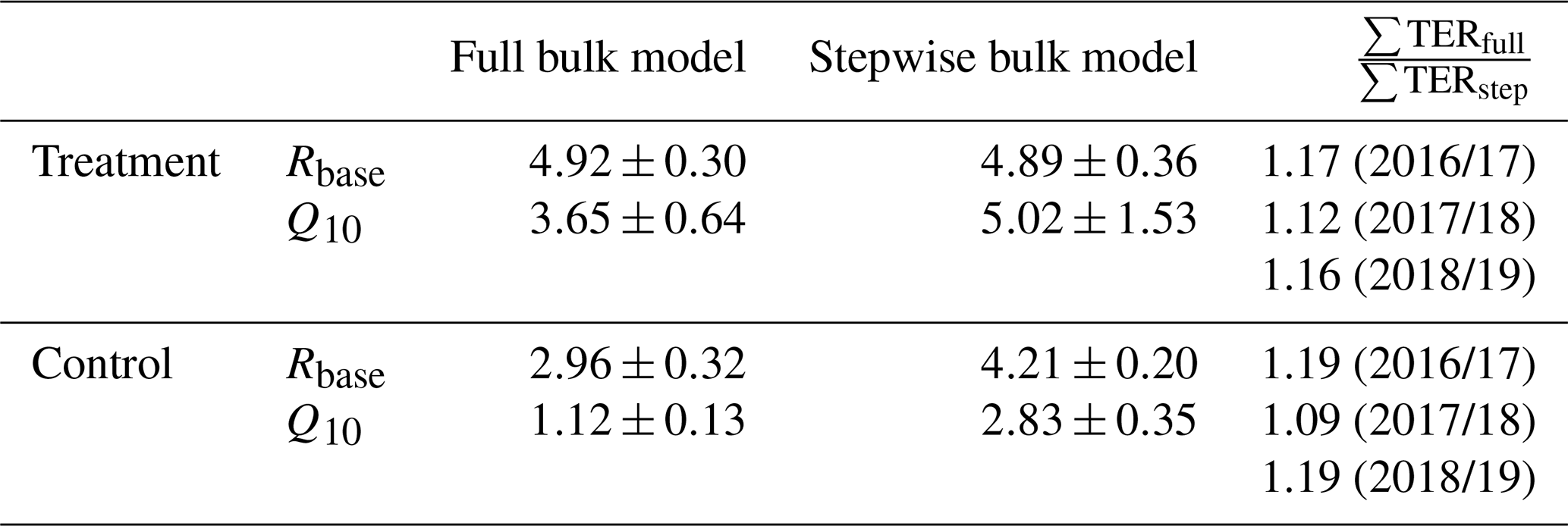

Figure D1Time series (a–c) of daily averaged hourly air temperature measurements inside (Ttreat) and outside (Tcont) warming treatment plots. The differences between Ttreat and Tcont are mostly positive. The distributions of the temperature differences including mean, median, and standard deviation (SD) are shown in (d–f).
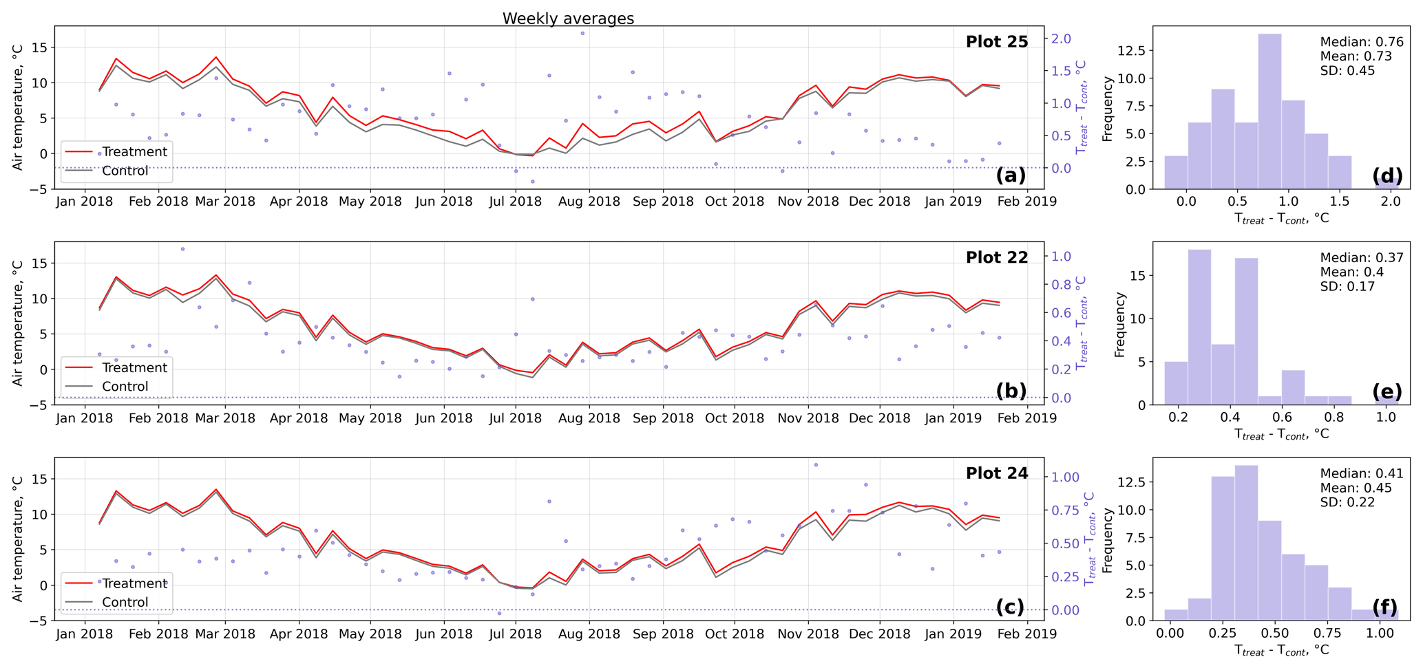
Figure D2Time series (a–c) of weekly averaged hourly air temperature measurements inside (Ttreat) and outside (Tcont) warming treatment plots. The differences between Ttreat and Tcont are mostly positive. The distributions of the temperature differences including mean, median, and standard deviation (SD) are shown in (d–f).
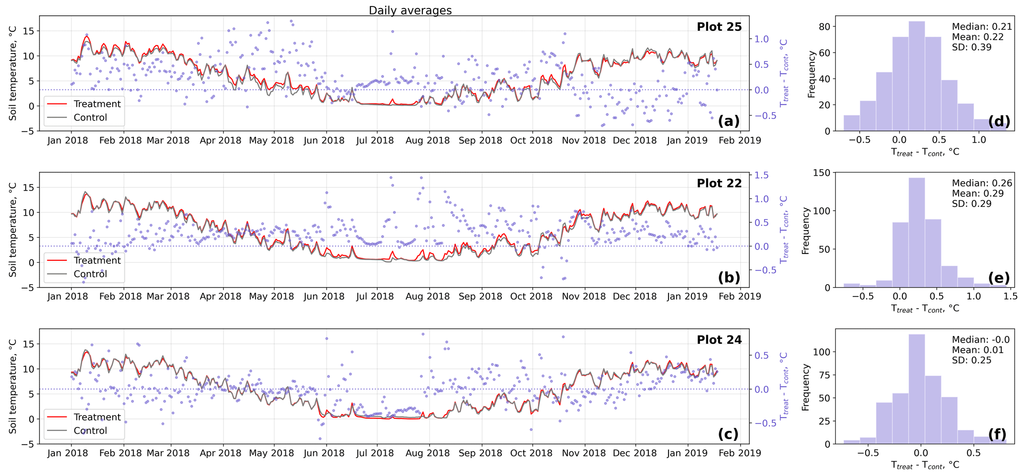
Figure D3Time series (a–c) of daily averaged hourly soil temperature measurements inside (Ttreat) and outside (Tcont) warming treatment plots. The differences between Ttreat and Tcont are mostly positive. The distributions of the temperature differences including mean, median, and standard deviation (SD) are shown in (d–f).
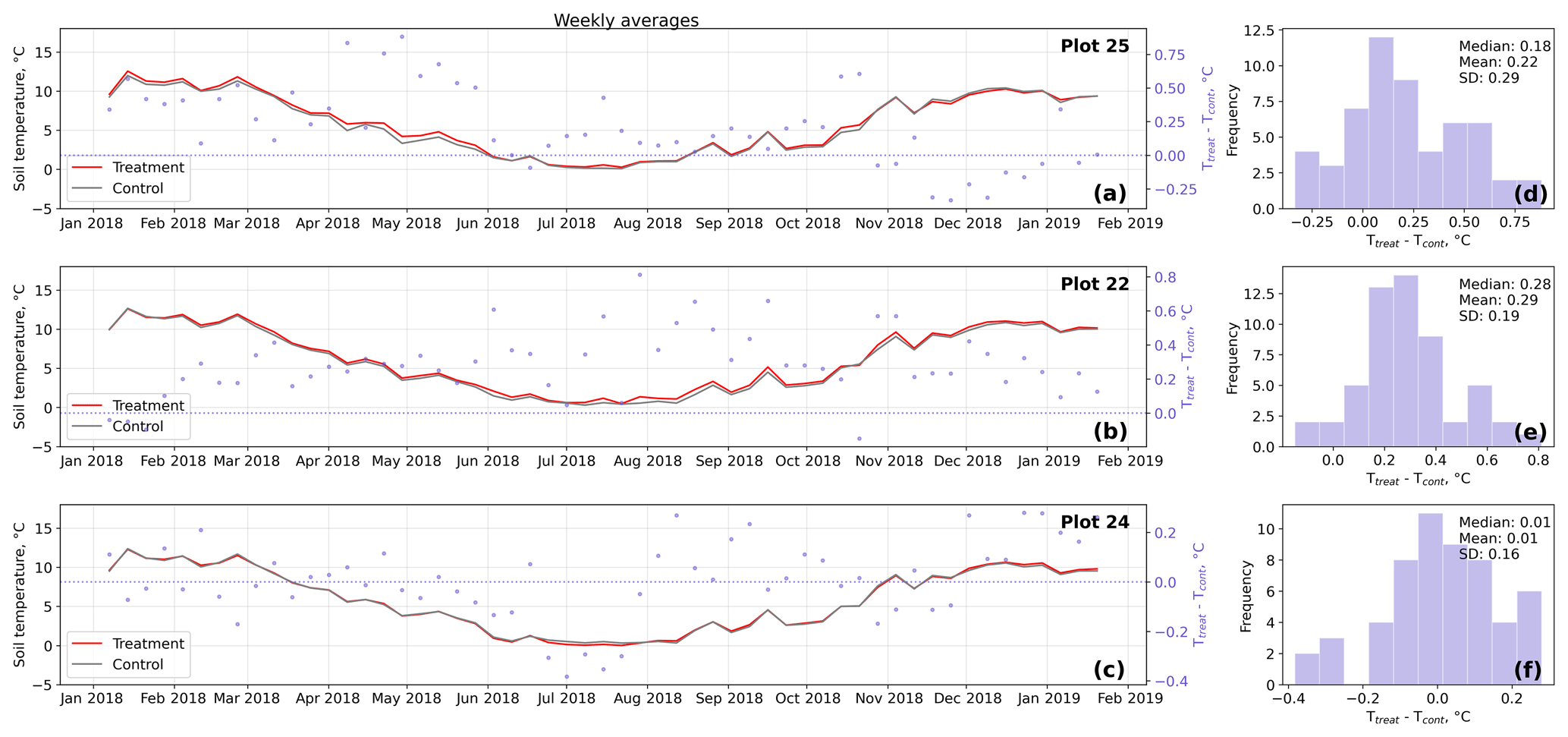
Figure D4Time series (a–c) of weekly averaged hourly soil temperature measurements inside (Ttreat) and outside (Tcont) warming treatment plots. The differences between Ttreat and Tcont are mostly positive. The distributions of the temperature differences including mean, median, and standard deviation (SD) are shown in (d–f).
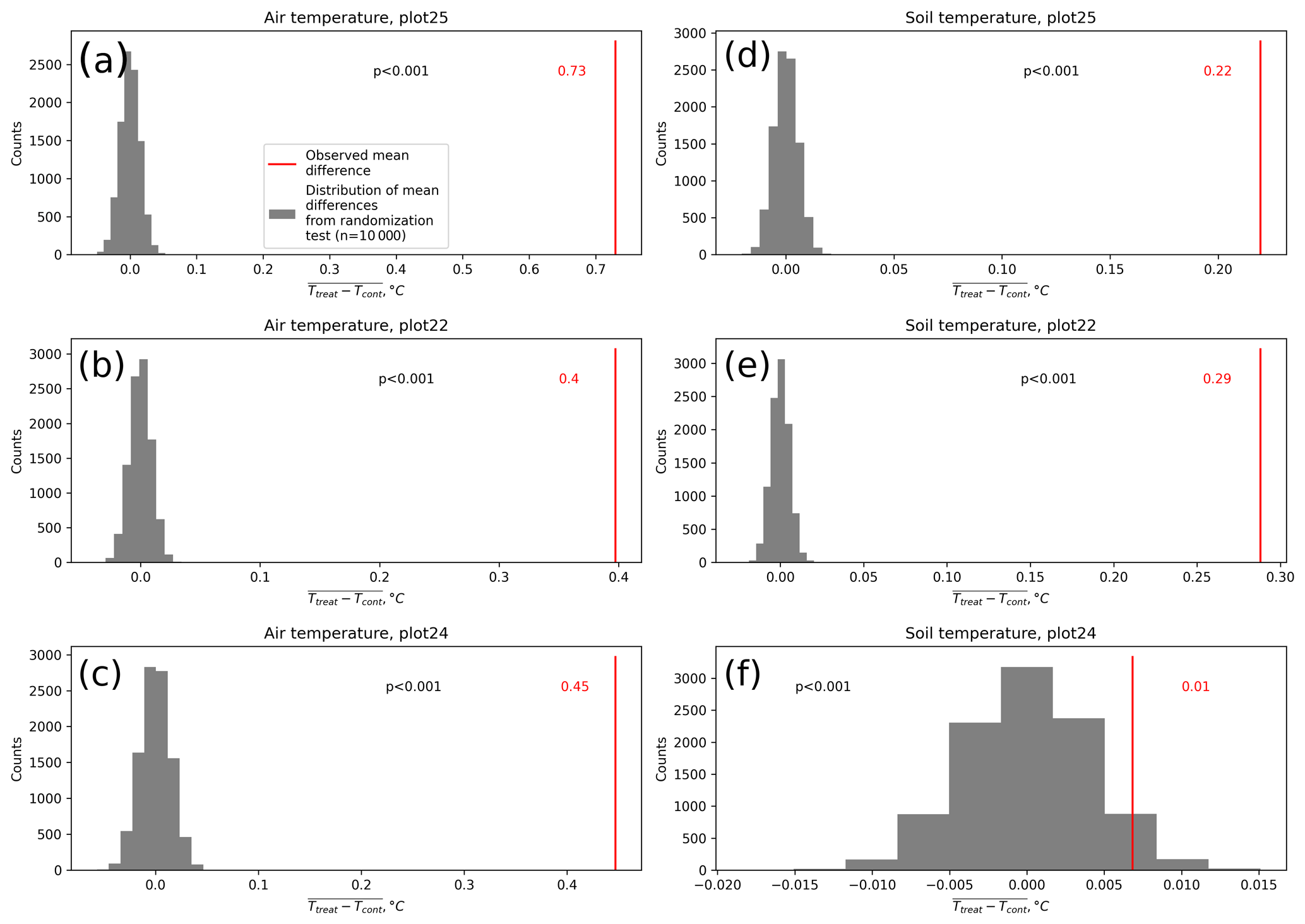
Figure D5Results of the randomization test we performed to check if the average differences between temperatures at the treatment and control plots are likely to be caused by random noise rather than by a systematic distinction between the conditions inside and outside the treatment plots.
We published the code here: https://doi.org/10.5281/zenodo.5196131 (Holl et al., 2021).
We published our data sets here: https://doi.org/10.1594/PANGAEA.934718 (Pancotto et al., 2021a) and https://doi.org/10.1594/PANGAEA.934731 (Pancotto et al., 2021b).
The supplement related to this article is available online at: https://doi.org/10.5194/bg-18-4817-2021-supplement.
VP and LK conceptualized and administered the planning of the research activity and acquired the funds for it. VP, MFC, and JE conducted the fieldwork. VP and DH conducted literature research. DH and VP analyzed the data, created visualizations, and wrote the original draft. VP, DH, and LK reviewed and edited the original draft.
The authors declare that they have no conflict of interest.
Publisher's note: Copernicus Publications remains neutral with regard to jurisdictional claims in published maps and institutional affiliations.
For facilitating and greatly supporting our fieldwork we want to cordially thank Wiebke Münchberger, Till Kleinebecker, Christian Blodau, Mauro Britos Navarro, and Norman Rüggen. We thank Prefectura Naval Argentina for granting us permission to work on their property and for kindly inviting us to benefit from their facilities at the field site.
This work was supported by the Cluster of Excellence CliSAP (EXC177), Universität Hamburg, funded by the German Research Foundation (DFG); by the CONICET–MINCyT–DFG international cooperation grant 3829/15; by grant PIDUNTDF 15/16 of the Universidad Nacional de Tierra del Fuego, Antártida e Islas del Atlántico Sur (UNTDF); and by the DFG project KU 1418/6-1.
This paper was edited by Trevor Keenan and reviewed by Gerald Jurasinski and Tariq Munir.
Alexandrov, G. A., Brovkin, V. A., Kleinen, T., and Yu, Z.: The capacity of northern peatlands for long-term carbon sequestration, Biogeosciences, 17, 47–54, https://doi.org/10.5194/bg-17-47-2020, 2020. a
Aronson, E. L. and McNulty, S. G.: Appropriate experimental ecosystem warming methods by ecosystem, objective, and practicality, Agr. Forest Meteorol., 149, 1791–1799, https://doi.org/10.1016/j.agrformet.2009.06.007, 2009. a, b, c
Barnes, J. D., Balaguer, L., Manrique, E., Elvira, S., and Davison, A. W.: A reappraisal of the use of DMSO for the extraction and determination of chlorophylls, Environ. Exp. Bot., 32, 85–100, 1992. a
Biasi, C., Meyer, H., Rusalimova, O., Hämmerle, R., Kaiser, C., Baranyi, C., Daims, H., Lashchinsky, N., Barsukov, P., and Richter, A.: Initial effects of experimental warming on carbon exchange rates, plant growth and microbial dynamics of a lichen-rich dwarf shrub tundra in Siberia, Plant Soil, 307, 191–205, https://doi.org/10.1007/s11104-008-9596-2, 2008. a
Bokhorst, S., Huiskes, A., Convey, P., and Aerts, R.: The effect of environmental change on vascular plant and cryptogam communities from the Falkland Islands and the Maritime Antarctic, BMC Ecol., 7, 1–13, https://doi.org/10.1186/1472-6785-7-15, 2007. a, b, c, d
Bokhorst, S., Bjerke, J. W., Davey, M. P., Taulavuori, K., Taulavuori, E., Laine, K., Callaghan, T. V., and Phoenix, G. K.: Impacts of extreme winter warming events on plant physiology in a sub-Arctic heath community, Physiol. Plantarum, 140, 128–140, https://doi.org/10.1111/j.1399-3054.2010.01386.x, 2010. a, b
Bokhorst, S., Huiskes, A., Convey, P., Sinclair, B. J., Lebouvier, M., Van de Vijver, B., and Wall, D. H.: Microclimate impacts of passive warming methods in Antarctica: Implications for climate change studies, Polar Biol., 34, 1421–1435, https://doi.org/10.1007/s00300-011-0997-y, 2011. a
Broder, T., Blodau, C., Biester, H., and Knorr, K. H.: Peat decomposition records in three pristine ombrotrophic bogs in southern Patagonia, Biogeosciences, 9, 1479–1491, https://doi.org/10.5194/bg-9-1479-2012, 2012. a
Broder, T., Blodau, C., Biester, H., and Knorr, K. H.: Sea spray, trace elements, and decomposition patterns as possible constraints on the evolution of CH4 and CO2 concentrations and isotopic signatures in oceanic ombrotrophic bogs, Biogeochemistry, 122, 327–342, https://doi.org/10.1007/s10533-014-0044-5, 2015. a
Brooks, A. and Farquhar, G. D.: Effect of temperature on the CO2/O2 specificity of ribulose-1,5-bisphosphate carboxylase/oxygenase and the rate of respiration in the light, Planta, 165, 397–406, 1985. a
Chapin, F. S., Matson, P. A., and Vitousek, P. M.: Principles of Terrestrial Ecosystem Ecology, Springer New York, New York, NY, https://doi.org/10.1007/978-1-4419-9504-9, 2011. a
Day, T. A., Ruhland, C. T., and Xiong, F. S.: Influence of solar ultraviolet-B radiation on Antarctic terrestrial plants: Results from a 4 year field study, J. Photoch. Photobio. B, 62, 78–87, https://doi.org/10.1016/S1011-1344(01)00161-0, 2001. a
Day, T. A., Ruhland, C. T., and Xiong, F. S.: Warming increases aboveground plant biomass and C stocks in vascular-plant-dominated Antarctic tundra, Glob. Change Biol., 14, 1827–1843, https://doi.org/10.1111/j.1365-2486.2008.01623.x, 2008. a
Dusenge, M. E., Duarte, A. G., and Way, D. A.: Plant carbon metabolism and climate change: elevated CO2 and temperature impacts on photosynthesis, photorespiration and respiration, New Phytol., 221, 32–49, https://doi.org/10.1111/nph.15283, 2019. a
Eckhardt, T. and Kutzbach, L.: MATLAB code to calculate gas fluxes from chamber-based methods, PANGAEA [code], https://doi.org/10.1594/PANGAEA.857799, 2016. a
Edgington, E. and Onghena, P.: Randomization Tests, Fourth Edition, Statistics: A Series of Textbooks and Monographs, Taylor & Francis, New York, 2007. a
Fan, X., Duan, Q., Shen, C., Wu, Y., and Xing, C.: Global surface air temperatures in CMIP6: historical performance and future changes, Environ. Res. Lett., 15, 104 056, https://doi.org/10.1088/1748-9326/abb051, 2020. a
Fritz, C., Pancotto, V. A., Elzenga, J. T., Visser, E. J., Grootjans, A. P., Pol, A., Iturraspe, R., Roelofs, J. G., and Smolders, A. J.: Zero methane emission bogs: Extreme rhizosphere oxygenation by cushion plants in Patagonia, New Phytol., 190, 398–408, https://doi.org/10.1111/j.1469-8137.2010.03604.x, 2011. a, b, c
Gallego-Sala, A. V., Charman, D. J., Brewer, S., Page, S. E., Prentice, I. C., Friedlingstein, P., Moreton, S., Amesbury, M. J., Beilman, D. W., Björck, S., Blyakharchuk, T., Bochicchio, C., Booth, R. K., Bunbury, J., Camill, P., Carless, D., Chimner, R. A., Clifford, M., Cressey, E., Courtney-Mustaphi, C., De Vleeschouwer, F., de Jong, R., Fialkiewicz-Koziel, B., Finkelstein, S. A., Garneau, M., Githumbi, E., Hribjlan, J., Holmquist, J., Hughes, P. D., Jones, C., Jones, M. C., Karofeld, E., Klein, E. S., Kokfelt, U., Korhola, A., Lacourse, T., Le Roux, G., Lamentowicz, M., Large, D., Lavoie, M., Loisel, J., Mackay, H., MacDonald, G. M., Makila, M., Magnan, G., Marchant, R., Marcisz, K., Martínez Cortizas, A., Massa, C., Mathijssen, P., Mauquoy, D., Mighall, T., Mitchell, F. J., Moss, P., Nichols, J., Oksanen, P. O., Orme, L., Packalen, M. S., Robinson, S., Roland, T. P., Sanderson, N. K., Sannel, A. B. K., Silva-Sánchez, N., Steinberg, N., Swindles, G. T., Turner, T. E., Uglow, J., Väliranta, M., van Bellen, S., van der Linden, M., van Geel, B., Wang, G., Yu, Z., Zaragoza-Castells, J., and Zhao, Y.: Latitudinal limits to the predicted increase of the peatland carbon sink with warming, Nat. Clim. Change, 8, 907–913, https://doi.org/10.1038/s41558-018-0271-1, 2018. a
Gorham, E.: Northern peatlands: role in the carbon cycle and probable responses to climatic warming, Ecol. Appl., 1, 182–195, https://doi.org/10.2307/1941811, 1991. a
Grootjans, A., Iturraspe, R., Lanting, A., Fritz, C., and Joosten, H.: Ecohydrological features of some contrasting mires in Tierra del Fuego, Mires and Peat, Argentina, 6, 1–15, 2010. a
Heskel, M. A., Atkin, O. K., Turnbull, M. H., and Griffin, K. L.: Bringing the Kok effect to light: A review on the integration of daytime respiration and net ecosystem exchange, Ecosphere, 4, 1–14, https://doi.org/10.1890/ES13-00120.1, 2013. a
Holl, D., Pancotto, V., Heger, A., Camargo, S. J., and Kutzbach, L.: Cushion bogs are stronger carbon dioxide net sinks than moss-dominated bogs as revealed by eddy covariance measurements on Tierra del Fuego, Argentina, Biogeosciences, 16, 3397–3423, https://doi.org/10.5194/bg-16-3397-2019, 2019. a, b, c, d, e
Holl, D.: DavidHoll/ExpWarmingTdF: CO2 flux modeling based on chamber flux measurements from a warming experiment on Tierra del Fuego, Argentina (v1.0.0), Zenodo [code], https://doi.org/10.5281/zenodo.5196131, 2021. a
Hopple, A. M., Wilson, R. M., Kolton, M., Zalman, C. A., Chanton, J. P., Kostka, J., Hanson, P. J., Keller, J. K., and Bridgham, S. D.: Massive peatland carbon banks vulnerable to rising temperatures, Nat. Commun., 11, 4–10, https://doi.org/10.1038/s41467-020-16311-8, 2020. a
Iturraspe, R.: Spatial analysis and description of eastern peatlands of Tierra del Fuego, Argentina, in: Mires from Pole to Pole, edited by: Lindholm, T., Heikkilä, R., and Ympäristökeskus, S., 385–389, Finnish Environment Inst., Helsinki, 2012. a, b
Kleinebecker, T., Hölzel, N., and Vogel, A.: Gradients of continentality and moisture in South Patagonian ombrotrophic peatland vegetation, Folia Geobot., 42, 363–382, 2007. a
Kleinebecker, T., Hölzel, N., and Vogel, A.: South Patagonian ombrotrophic bog vegetation reflects biogeochemical gradients at the landscape level, Journal of Vegetation Science, 19, 151–160, 2008. a
Kutzbach, L.: AmeriFlux AR-TF1 Rio Moat bog, Ver. 2-5, AmeriFlux AMP [data set], https://doi.org/10.17190/AMF/1543389, 2021. a
Laine, A. M., Mäkiranta, P., Laiho, R., Mehtätalo, L., Penttilä, T., Korrensalo, A., Minkkinen, K., Fritze, H., and Tuittila, E.-S.: Warming impacts on boreal fen CO2 exchange under wet and dry conditions, Glob. Change Biol., 25, 1995–2008, https://doi.org/10.1111/gcb.14617, 2019. a
Liancourt, P., Sharkhuu, A., Ariuntsetseg, L., Boldgiv, B., Helliker, B. R., Plante, A. F., Petraitis, P. S., and Casper, B. B.: Temporal and spatial variation in how vegetation alters the soil moisture response to climate manipulation, Plant Soil, 351, 249–261, https://doi.org/10.1007/s11104-011-0956-y, 2012. a
Livensperger, C., Steltzer, H., Darrouzet-Nardi, A., Sullivan, P. F., Wallenstein, M., and Weintraub, M. N.: Earlier snowmelt and warming lead to earlier but not necessarily more plant growth, AoB PLANTS, 8, 1–15, https://doi.org/10.1093/aobpla/plw021, 2016. a
Livingston, G. and Hutchinson, G.: Enclosure-based measurement of trace gas exchange: applications and sources of error, in: Biogenic trace gases: measuring emissions from soil and water, 51, 14–51, Blackwell Science, Cambridge, 1995. a
Lyons, C. L., Branfireun, B. A., McLaughlin, J., and Lindo, Z.: Simulated climate warming increases plant community heterogeneity in two types of boreal peatlands in north–central Canada, Journal of Vegetation Science, 31, 908–919, https://doi.org/10.1111/jvs.12912, 2020. a
Mahecha, M. D., Reichstein, M., Carvalhais, N., Lasslop, G., Lange, H., Seneviratne, S. I., Vargas, R., Ammann, C., Arain, M. A., Cescatti, A., Janssens, I. A., Migliavacca, M., Montagnani, L., and Richardson, A. D.: Global Convergence in the Temperature Sensitivity of Respiration at Ecosystem Level, Science, 329, 838–840, 2010. a
Mäkiranta, P., Laiho, R., Mehtätalo, L., Straková, P., Sormunen, J., Minkkinen, K., Penttilä, T., Fritze, H., and Tuittila, E.-S.: Responses of phenology and biomass production of boreal fens to climate warming under different water-table level regimes, Glob. Change Biol., 24, 944–956, https://doi.org/10.1111/gcb.13934, 2017. a
Malhotra, A., Brice, D. J., Childs, J., Graham, J. D., Hobbie, E. A., Vander Stel, H., Feron, S. C., Hanson, P. J., and Iversen, C. M.: Peatland warming strongly increases fine-root growth, Proc. Natl. Acad. Sci. USA, 117, 17627–17634, https://doi.org/10.1073/pnas.2003361117, 2020. a, b
Marion, G. M., Henry, G. H., Freckman, D. W., Johnstone, J., Jones, G., Jones, M. H., Lévesque, E., Molau, U., Mølgaard, P., Parsons, A. N., Svoboda, J., and Virginia, R. A.: Open-top designs for manipulating field temperature in high-latitude ecosystems, Glob. Change Biol., 3, 20–32, https://doi.org/10.1111/j.1365-2486.1997.gcb136.x, 1997. a, b, c, d, e
Münchberger, W., Knorr, K.-H., Blodau, C., Pancotto, V. A., and Kleinebecker, T.: Zero to moderate methane emissions in a densely rooted, pristine Patagonian bog – biogeochemical controls as revealed from isotopic evidence, Biogeosciences, 16, 541–559, https://doi.org/10.5194/bg-16-541-2019, 2019. a, b, c
Munir, T. M., Perkins, M., Kaing, E., and Strack, M.: Carbon dioxide flux and net primary production of a boreal treed bog: Responses to warming and water-table-lowering simulations of climate change, Biogeosciences, 12, 1091–1111, https://doi.org/10.5194/bg-12-1091-2015, 2015. a, b
Munir, T. M., Khadka, B., Xu, B., and Strack, M.: Mineral nitrogen and phosphorus pools affected by water table lowering and warming in a boreal forested peatland, Ecohydrology, 10, e1893, https://doi.org/10.1002/eco.1893, 2017. a
Pancotto, V., Holl, D., Escobar, J., and Kutzbach, L.: Temperature measurements from treatment and control plots of a passive warming experiment at a cushion bog on Tierra del Fuego, Argentina, PANGAEA [data set], https://doi.org/10.1594/PANGAEA.934731, 2021a. a
Pancotto, V., Holl, D., Escobar, J., and Kutzbach, L.: Carbon dioxide fluxes from treatment and control plots of a passive warming experiment at a cushion bog on Tierra del Fuego, Argentina, PANGAEA [data set], https://doi.org/10.1594/PANGAEA.934718, 2021b. a
Parish, F., Sirin, A., Charman, D., Joosten, H., Minaeva, T., and Silvius, M.: Assessment on peatlands, biodiversity and climate change, Global Environment Centre, Kuala Lumpur, 2008. a
Peñuelas, J., Gordon, C., Llorens, L., Nielsen, T., Tietema, A., Beier, C., Bruna, P., Emmett, B., Estiarte, M., and Gorissen, A.: Nonintrusive field experiments show different plant responses to warming and drought among sites, seasons, and species in a north-south European gradient, Ecosystems, 7, 598–612, https://doi.org/10.1007/s10021-004-0179-7, 2004. a
Pérez-Harguindeguy, N., Díaz, S., Garnier, E., Lavorel, S., Poorter, H., Jaureguiberry, P., Cornwell, W. K., Craine, J. M., Gurvich, D. E., Urcelay, C., Veneklaas, E. J., Reich, P. B., Poorter, L., Wright, I. J., Ray, P., Enrico, L., Pausas, J. G., Vos, A. C. D., Buchmann, N., Funes, G., Quétier, F., Hodgson, J. G., Thompson, K., Morgan, H. D., Steege, H., Heijden, M. G. A. V. D., Sack, L., Blonder, B., Poschlod, P., Vaieretti, M. V., Conti, G., Staver, A. C., Aquino, S., and Cornelissen, J. H. C.: New handbook for standardised measurement of plant functional traits worldwide, Aust. J. Bot., 64, 715–716, https://doi.org/10.1071/BT12225, 2016. a
Ponce, J. F. and Fernández, M.: Climatic and environmental history of Isla de los Estados, Argentina, Springer, New York, 2014. a
Prather, H. M., Casanova-Katny, A., Clements, A. F., Chmielewski, M. W., Balkan, M. A., Shortlidge, E. E., Rosenstiel, T. N., and Eppley, S. M.: Species-specific effects of passive warming in an Antarctic moss system, Roy. Soc. Open Sci., 6, 190744, https://doi.org/10.1098/rsos.190744, 2019. a, b
Robson, T. M., Pancotto, V. A., Flint, S. D., Ballaré, C. L., Sala, O. E., Scopel, A. L., and Caldwell, M. M.: Six years of solar UV-B manipulations affect growth of Sphagnum and vascular plants in a Tierra del Fuego peatland, New Phytol., 160, 379–389, https://doi.org/10.1046/j.1469-8137.2003.00898.x, 2003. a
Rousseaux, M. C., Scopel, A. L., Searles, P. S., Caldwell, M. M., Sala, O. E., and Ballaré, C. L.: Responses to solar ultraviolet-B radiation in a shrub-dominated natural ecosystem of Tierra del Fuego (southern Argentina), Glob. Change Biol., 7, 467–478, https://doi.org/10.1046/j.1365-2486.2001.00413.x, 2001. a
Rueden, C. T., Schindelin, J., Hiner, M. C., DeZonia, B. E., Walter, A. E., Arena, E. T., and Eliceiri, K. W.: ImageJ2: ImageJ for the next generation of scientific image data, BMC Bioinformatics, 18, 1–26, https://doi.org/10.1186/s12859-017-1934-z, 2017. a
Runkle, B. R. K., Sachs, T., Wille, C., Pfeiffer, E.-M., and Kutzbach, L.: Bulk partitioning the growing season net ecosystem exchange of CO2 in Siberian tundra reveals the seasonality of its carbon sequestration strength, Biogeosciences, 10, 1337–1349, https://doi.org/10.5194/bg-10-1337-2013, 2013. a
Rustad, L. E., Campbell, J. L., Marion, G. M., Norby, R. J., Mitchell, M. J., Hartley, A. E., Cornelissen, J. H., Gurevitch, J., Alward, R., Beier, C., Burke, I., Canadell, J., Callaghan, T., Christensen, T. R., Fahnestock, J., Fernandez, I., Harte, J., Hollister, R., John, H., Ineson, P., Johnson, M. G., Jonasson, S., John, L., Linder, S., Lukewille, A., Masters, G., Melillo, J., Mickelsen, A., Neill, C., Olszyk, D. M., Press, M., Pregitzer, K., Robinson, C., Rygiewiez, P. T., Sala, O., Schmidt, I. K., Shaver, G., Thompson, K., Tingey, D. T., Verburg, P., Wall, D., Welker, J., and Wright, R.: A meta-analysis of the response of soil respiration, net nitrogen mineralization, and aboveground plant growth to experimental ecosystem warming, Oecologia, 126, 543–562, https://doi.org/10.1007/s004420000544, 2001. a
Santana, A., Porter, C., Butorovic, N., and Olave, C.: Primeros Antecedentes Climatológicos De Estaciones (Aws) En El Canal Beagle, Anales Instituto Patagonia (Chile), 34, 5–20, 2006. a
Searles, P. S., Flint, S. D., Díaz, S. B., Rousseaux, M. C., Ballaré, C. L., and Caldwell, M. M.: Plant response to solar ultraviolet-B radiation in a southern South American Sphagnum peatland, J. Ecol., 90, 704–713, https://doi.org/10.1046/j.1365-2745.2002.00709.x, 2002. a
Sharkhuu, A., Plante, A. F., Enkhmandal, O., Casper, B. B., Helliker, B. R., Boldgiv, B., and Petraitis, P. S.: Effects of open-top passive warming chambers on soil respiration in the semi-arid steppe to taiga forest transition zone in Northern Mongolia, Biogeochemistry, 115, 333–348, https://doi.org/10.1007/s10533-013-9839-z, 2013. a
Strack, M., Munir, T. M., and Khadka, B.: Shrub abundance contributes to shifts in dissolved organic carbon concentration and chemistry in a continental bog exposed to drainage and warming, Ecohydrology, 12, e2100, https://doi.org/10.1002/eco.2100, 2019. a
Tuhkanen, S.: The climate of Tierra del Fuego from a vegetation geographical point of view and its ecoclimatic counterparts elsewhere, Finnish Botanical Publishing Board, Helsinki, 1992. a
van Bellen, S., Mauquoy, D., Hughes, P. D., Roland, T. P., Daley, T. J., Loader, N. J., Street-Perrott, F. A., Rice, E. M., Pancotto, V. A., and Payne, R. J.: Late-Holocene climate dynamics recorded in the peat bogs of Tierra del Fuego, South America, Holocene, 26, 489–501, https://doi.org/10.1177/0959683615609756, 2016. a
Virtanen, P., Gommers, R., Oliphant, T. E., Haberland, M., Reddy, T., Cournapeau, D., Burovski, E., Peterson, P., Weckesser, W., Bright, J., van der Walt, S. J., Brett, M., Wilson, J., Millman, K. J., Mayorov, N., Nelson, A. R., Jones, E., Kern, R., Larson, E., Carey, C. J., Polat, I., Feng, Y., Moore, E. W., VanderPlas, J., Laxalde, D., Perktold, J., Cimrman, R., Henriksen, I., Quintero, E. A., Harris, C. R., Archibald, A. M., Ribeiro, A. H., Pedregosa, F., van Mulbregt, P., Vijaykumar, A., Bardelli, A. P., Rothberg, A., Hilboll, A., Kloeckner, A., Scopatz, A., Lee, A., Rokem, A., Woods, C. N., Fulton, C., Masson, C., Häggström, C., Fitzgerald, C., Nicholson, D. A., Hagen, D. R., Pasechnik, D. V., Olivetti, E., Martin, E., Wieser, E., Silva, F., Lenders, F., Wilhelm, F., Young, G., Price, G. A., Ingold, G. L., Allen, G. E., Lee, G. R., Audren, H., Probst, I., Dietrich, J. P., Silterra, J., Webber, J. T., Slavič, J., Nothman, J., Buchner, J., Kulick, J., Schönberger, J. L., de Miranda Cardoso, J. V., Reimer, J., Harrington, J., Rodríguez, J. L. C., Nunez-Iglesias, J., Kuczynski, J., Tritz, K., Thoma, M., Newville, M., Kümmerer, M., Bolingbroke, M., Tartre, M., Pak, M., Smith, N. J., Nowaczyk, N., Shebanov, N., Pavlyk, O., Brodtkorb, P. A., Lee, P., McGibbon, R. T., Feldbauer, R., Lewis, S., Tygier, S., Sievert, S., Vigna, S., Peterson, S., More, S., Pudlik, T., Oshima, T., Pingel, T. J., Robitaille, T. P., Spura, T., Jones, T. R., Cera, T., Leslie, T., Zito, T., Krauss, T., Upadhyay, U., Halchenko, Y. O., and Vázquez-Baeza, Y.: SciPy 1.0: fundamental algorithms for scientific computing in Python, Nat. Methods, 17, 261–272, https://doi.org/10.1038/s41592-019-0686-2, 2020. a, b
Walker, M. D., Wahren, C. H., Hollister, R. D., Henry, G. H., Ahlquist, L. E., Alatalo, J. M., Bret-Harte, M. S., Calef, M. P., Callaghan, T. V., Carroll, A. B., Epstein, H. E., Jónsdóttir, I. S., Klein, J. A., Magnússon, B., Molau, U., Oberbauer, S. F., Rewa, S. P., Robinson, C. H., Shaver, G. R., Suding, K. N., Thompson, C. C., Tolvanen, A., Totland, Ø., Turner, P. L., Tweedie, C. E., Webber, P. J., and Wookey, P. A.: Plant community responses to experimental warming across the tundra biome, Proc. Natl. Acad. Sci. USA, 103, 1342–1346, https://doi.org/10.1073/pnas.0503198103, 2006. a, b, c
Wellburn, A.: The spectral determination of chlorophylls a and b, as well as total carotenoids, using various solvents with spectrophotometers of different resolution, J. Plant Physiol., 144, 307–313, 1994. a, b
Wieners, K.-H., Giorgetta, M., Jungclaus, J., Reick, C., Esch, M., Bittner, M., Gayler, V., Haak, H., de Vrese, P., Raddatz, T., Mauritsen, T., von Storch, J.-S., Behrens, J., Brovkin, V., Claussen, M., Crueger, T., Fast, I., Fiedler, S., Hagemann, S., Hohenegger, C., Jahns, T., Kloster, S., Kinne, S., Lasslop, G., Kornblueh, L., Marotzke, J., Matei, D., Meraner, K., Mikolajewicz, U., Modali, K., Müller, W., Nabel, J., Notz, D., Peters, K., Pincus, R., Pohlmann, H., Pongratz, J., Rast, S., Schmidt, H., Schnur, R., Schulzweida, U., Six, K., Stevens, B., Voigt, A., and Roeckner, E.: MPI-M MPI-ESM1.2-LR model output prepared for CMIP6 ScenarioMIP ssp126. Version 20210323, https://doi.org/10.22033/ESGF/CMIP6.6690, 2019a. a
Wieners, K.-H., Giorgetta, M., Jungclaus, J., Reick, C., Esch, M., Bittner, M., Gayler, V., Haak, H., de Vrese, P., Raddatz, T., Mauritsen, T., von Storch, J.-S., Behrens, J., Brovkin, V., Claussen, M., Crueger, T., Fast, I., Fiedler, S., Hagemann, S., Hohenegger, C., Jahns, T., Kloster, S., Kinne, S., Lasslop, G., Kornblueh, L., Marotzke, J., Matei, D., Meraner, K., Mikolajewicz, U., Modali, K., Müller, W., Nabel, J., Notz, D., Peters, K., Pincus, R., Pohlmann, H., Pongratz, J., Rast, S., Schmidt, H., Schnur, R., Schulzweida, U., Six, K., Stevens, B., Voigt, A., and Roeckner, E.: MPI-M MPI-ESM1.2-LR model output prepared for CMIP6 ScenarioMIP ssp585. Version 20210323, https://doi.org/10.22033/ESGF/CMIP6.6705, 2019b. a
Wilson, R. M., Hopple, A. M., Tfaily, M. M., Sebestyen, S. D., Schadt, C. W., Pfeifer-Meister, L., Medvedeff, C., Mcfarlane, K. J., Kostka, J. E., Kolton, M., Kolka, R. K., Kluber, L. A., Keller, J. K., Guilderson, T. P., Griffiths, N. A., Chanton, J. P., Bridgham, S. D., and Hanson, P. J.: Stability of peatland carbon to rising temperatures, Nat. Commun., 7, 1–10, https://doi.org/10.1038/ncomms13723, 2016. a
Yu, Z., Loisel, J., Brosseau, D. P., Beilman, D. W., and Hunt, S. J.: Global peatland dynamics since the Last Glacial Maximum, Geophys. Res. Lett., 37, 1–5, https://doi.org/10.1029/2010GL043584, 2010. a
Zaller, J. G., Caldwell, M. M., Flint, S. D., Ballaré, C. L., Scopel, A. L., and Sala, O. E.: Solar UVB and warming affect decomposition and earthworms in a fen ecosystem in Tierra del Fuego, Argentina, Glob. Change Biol., 15, 2493–2502, https://doi.org/10.1111/j.1365-2486.2009.01970.x, 2009. a, b
Zhang, Z., Zhang, R., Cescatti, A., Wohlfahrt, G., Buchmann, N., Zhu, J., Chen, G., Moyano, F., Pumpanen, J., Hirano, T., Takagi, K., and Merbold, L.: Effect of climate warming on the annual terrestrial net ecosystem CO2 exchange globally in the boreal and temperate regions, Sci. Rep., 7, 1–11, https://doi.org/10.1038/s41598-017-03386-5, 2017. a
- Abstract
- Introduction
- Material and methods
- Results
- Discussion
- Conclusions
- Appendix A: Flux measurement statistics
- Appendix B: Site conditions and vegetation properties
- Appendix C: Comparison of NEE model parameter estimates obtained with different models and with different measurement techniques
- Appendix D: Time series of air and soil temperatures inside and outside the warming treatment
- Code availability
- Data availability
- Author contributions
- Competing interests
- Disclaimer
- Acknowledgements
- Financial support
- Review statement
- References
- Supplement