Field-scale CH₄ emission at a subarctic mire with heterogeneous permafrost thaw status

The Arctic is exposed to even faster temperature changes than most other areas on Earth. Constantly increasing temperature will lead to thawing permafrost and changes in the methane (CH₄) emissions from wetlands. One of the places exposed to those changes is the Abisko–Stordalen Mire in northern Sweden, where climate and vegetation studies have been conducted since the 1970s.

In our study, we analyzed field-scale methane emissions measured by the eddy covariance method at Abisko–Stordalen Mire for 3 years (2014–2016). The site is a subarctic mire mosaic of palsas, thawing palsas, fully thawed fens, and open water bodies. A bimodal wind pattern prevalent at the site provides an ideal opportunity to measure mire patches with different permafrost status with one flux measurement system. The flux footprint for westerly winds was dominated by elevated palsa plateaus, while the footprint was almost equally distributed between palsas and thawing bog-like areas for easterly winds. As these patches are exposed to the same climatic and weather conditions, we analyzed the differences in the responses of their methane emission for environmental parameters.

The methane fluxes followed a similar annual cycle over the 3 study years, with a gentle rise during spring and a decrease during autumn, without emission bursts at either end of the ice-free season. The peak emission during the ice-free season differed significantly for the two mire areas with different permafrost status: the palsa mire emitted 19 mg-C m⁻² d⁻¹ and the thawing wet sector 40 mg-C m⁻² d⁻¹. Factors controlling the methane emission were analyzed using generalized linear models. The main driver for methane fluxes was peat temperature for both wind sectors. Soil water content above the water table emerged as an explanatory variable for the 3 years for western sectors and the year 2016 in the eastern sector. The water table level showed a significant correlation with methane emission for the year 2016 as well. Gross primary production, however, did not show a significant correlation with methane emissions.

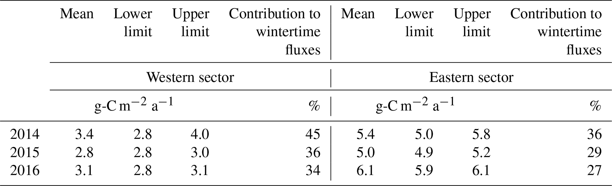
Annual methane emissions were estimated based on four different gap-filing methods. The different methods generally resulted in very similar annual emissions. The mean annual emission based on all models was 3.1 ± 0.3 g-C m⁻² a⁻¹ for the western sector and 5.5 ± 0.5 g-C m⁻² a⁻¹ for the eastern sector. The average annual emissions, derived from these data and a footprint climatology, were 2.7 ± 0.5 and 8.2 ± 1.5 g-C m⁻² a⁻¹ for the palsa and thawing surfaces, respectively. Winter fluxes were relatively high, contributing 27 %–45 % to the annual emissions.

1 Introduction

After a period of stabilization in the late 1990s to early 2000s, atmospheric methane (CH₄) concentration is increasing again at rates similar to those before 1993, which is approximately 12 ppb a⁻¹ (Dlugokencky et al., 2011; Nisbet et al., 2014; Saunois et al., 2020). The reasons behind this increase are still partly unclear, as the mechanisms that control the global CH₄ budget are not completely understood (Kirschke et al., 2013; Saunois et al., 2020). The largest natural source of CH₄ is wetlands, based on top-down emission estimates (Saunois et al., 2020), and this source may become stronger in the warming climate (Zhang et al., 2017). The shift in the isotopic composition of CH₄ towards more negative values also supports the hypothesis of changes in the biological source strength driving the increase in CH₄ concentration, as atmospheric CH₄ is becoming more ¹³C depleted (Nisbet et al., 2016).

Increasing temperature has shown to speed up the degradation of permafrost, which leads to losses in the soil carbon pool, often in the form of carbon dioxide (CO₂) and CH₄ (Malmer et al., 2005). The high northern latitudes are experiencing the fastest temperature increase due to the ongoing global warming. Temperature changes in the Arctic have been twice as high as the global average (Post et al., 2019).

Ecosystems near the annual near-surface air temperature isotherms of 0 ^∘C are vulnerable to permafrost thaw and changes in ecosystem characteristics in a warming climate. These vulnerable ecosystems include palsa mires, such as Stordalen Mire near Abisko, Sweden, where the recent warming has led to annual average temperatures exceeding 0 ^∘C since the 1980s (Callaghan et al., 2010, 2013; Post et al., 2019; Fig. S1). The warming has led to an acceleration of permafrost thaw processes and a transition from palsa plateaus, underlain by permafrost, to non-permafrost fen systems (Malmer et al., 2005). These deviations are likely to induce changes in biogeochemical processes, including increased CH₄ emissions (Christensen et al., 2003).

The most direct micrometeorological field-scale method used to measure CH₄ exchange between ecosystem and atmosphere is the eddy covariance (EC) method (e.g., Verma et al., 1986; Aubinet et al., 2012). The advantages of this method are its high temporal resolution and minimal disturbance to the measured surface. Thus, it is feasible for long-term measurements of rates of gas exchange that integrates over surface variation (Knox et al., 2016; Li et al., 2016; Rinne et al., 2018). However, information on the small-scale spatial distribution of surface fluxes is lost with the method due to the spatially integrative nature of the EC method. Instead of resolving the small-scale spatial variability, the EC method provides averaged fluxes from a larger area, the flux footprint area (Kljun et al., 2002). However, spatial variability can be resolved by the EC method using measurements conducted under different wind directions, as the footprint area is located upwind of the measurement tower. We can take advantage of this feature to obtain gas exchange rates from two different ecosystem types with one measurement system by placing the measurement system on the border between these systems (e.g., Jackowicz-Korczyński et al., 2010; Kowalska et al., 2013; Jammet et al., 2015, 2017). Stordalen Mire offers an excellent opportunity to conduct flux studies where one flux system is used to monitor two ecosystem types since the wind direction is bimodal. While previous studies in the area have compared open water surfaces to completely thawed fen (Jammet et al., 2015, 2017; Jansen et al., 2020), no comparison of field-scale CH₄ emission between permafrost palsa plateaus and thawing wet areas has been conducted yet.

Previous studies on CH₄ emission within the Stordalen Mire from areas with different permafrost status have been done using chamber measurements (McCalley et al., 2014; Deng et al., 2014). McCalley et al. (2014) reported CH₄ emissions from palsas underlain by permafrost to be close to zero and summertime emissions from thawing wet areas to be around 25 mg-C m⁻² d⁻², while completely thawed fen sites revealed much higher emission of 150 mg-C m⁻² d⁻². There are only few wintertime data on CH₄ emission available using the chamber method (Christensen et al., 2000; Nilsson et al., 2008; Godin et al., 2012; McCalley et al., 2014). However, EC measurements conducted at different northern mires typically show low but positive emissions in winter (Rinne et al., 2007; Yamulki et al., 2013, and others).

In this study we analyzed field-scale CH₄ emission from two areas of the Stordalen subarctic mire. The first area is dominated by drained permafrost plateau. The second area is thawing and thus resulting in wetter conditions. Outputs from this analysis are differences in the CH₄ emissions from the mire patches with heterogeneous permafrost status. We are expecting, based on the previous studies, that fluxes from the wetter sector will be around 30 mg-C m⁻² d⁻², while the palsa plateau will emit significantly lower fluxes during the peak season. We presume that winter fluxes will be positive but very low.

For estimation of annual CH₄ emission we need gap-free datasets. Up to date, there is no generally accepted gap-filling method for CH₄ fluxes; hence four different gap-filling methods were compared. The test of the four methods will decrease the uncertainty in the annual balance estimation (Hommeltenberg et al., 2014; Rößger et al., 2019; Kim et al., 2019). It was important to use more than one method in this case of study because datasets were portioned and due to that contained more gaps.

This study aimed to estimate the annual CH₄ emission from two distinct different ecotypes, with heterogeneous permafrost status, exposed to the same environmental factors. Furthermore, we analyzed the seasonal cycle of CH₄ emission to quantify the contribution during different seasons. Moreover, an analysis of differences in controlling factors for these two different areas was done.

2 Materials and method

2.1 Study site

The study area is Stordalen Mire, a mire complex underlain by discontinuous permafrost located in northern subarctic Sweden (68^∘20^′ N, 19^∘30^′ E) near Abisko (Ábeskovvu). The station Abisko–Stordalen (SE-Sto) is a part of the ICOS Sweden research infrastructure and is the only one in Sweden situated in the subarctic region. The measurement period that is analyzed here covers 3 years from 2014–2016. The mean annual near-surface air temperature in this region has been increasing during the last decades, and temperatures recorded by SMHI (Sveriges meteorologiska och hydrologiska institut) at ANS (Abisko naturvetenskapliga station) have exceeded the 0 ^∘C threshold since the late 1980s (Callaghan et al., 2013, Fig. S1). During the years 2014–2016, the mean near-surface air temperature (Ta) was 1.0 and 0.3 ^∘C at ANS and the ICOS Sweden station Abisko–Stordalen (SE-Sto), respectively. The average annual precipitation, based on ANS data, is around 330 mm a⁻¹. An acceleration of permafrost loss with increasing temperatures is likely (Callaghan et al., 2013).

The large mountain valley of Lake Torneträsk (Duortnosjávri) channels winds at the study site, leading to a bimodal wind distribution (Fig. 1), which allows us to divide our analyses into two distinct sectors. The plant community structure around the tower is determined by the hydrology, which in turn is determined by the microtopographic variation in the surface due to the local permafrost dynamics. Different plant communities would have different productivities, thus controlling the CO₂ and CH₄ fluxes from those surfaces. The area to the west of the EC mast is dominated by a drier permafrost palsa plateau, hereafter referred to as the western sector, whereas the area to the east is a mixture of thawing wet areas and palsas, hereafter referred to as the eastern sector. The drained permafrost plateau is dominated by Empetrum hermaphroditum, Betula nana, Rubus chamaemorus, Eriophorum vaginatum, Dicranum elongatum, and Sphagnum fuscum. The wet areas are characterizing by E. vaginatum, Carex rotundata, Sphagnum balticum, Drepanucladus schulzei, and Polytrichum jensenii (Johansson et al., 2006). The thawing areas in this sector exhibit ombrotrophic, bog-like, features. Dominant vegetation varies with the microforms of the mire.

Figure 1 The wind rose for the SE-Sto tower for years 2014–2016 for the daytime (a) and nighttime (b).

2.2 Flux measurements

The EC measurements of CH₄ fluxes at SE-Sto are made using a closed-path fast off-axis integrated cavity output spectrometer (OA-ICOS LGR model GGA-24EP, ABB Ltd, Zurich, Switzerland) combined with a 3-D sonic anemometer (SA-Metek uSonic-3 Class A, Metek GmbH, Germany). Air was sampled via a 29.6 m long polyethylene tubing with an 8.13 mm inner diameter. Analyses of the high-frequency loss were performed to assess the effect of relatively long sample tubing. We analyzed this with the co-spectra of the CH₄ and the vertical wind speed w. The analysis did not show a dampening effect at the high frequencies (Fig. S2); thus, the high frequency attenuation does not seem to be very large. Furthermore, the post-processing software we used to calculate fluxes includes correction for high-frequency losses. The nominal tube flow rate was 36 L min⁻¹. The sampling inlet was displaced 22 cm horizontally of the sonic anemometer measurement volume towards 180^∘. The response time of the Los Gatos Research (LGR) fast greenhouse gas analyzer (FGGA) was 0.1 s. The LGR FGGA was placed inside a heated and air-conditioned shelter. The anemometer was located north of the instrument shelter and was oriented with the sensors north pointing towards 186^∘. This orientation allows undisturbed wind measurements from both main wind directions, east and west.

CO₂ and H₂O were measured with a LI-COR LI-7200 (LI-COR Environment, USA) closed-path infrared gas analyzer. The sampling inlet was at the same location as the sampling point for the CH₄ analyzer. Sampled air was transported through 1.05 m and of 5.3 mm ID tubing. The nominal tube flow rate was 15 L min⁻¹.

The anemometer and air sampling tubes were mounted on a mast of 2.2 m above ground level (a.g.l.) (68^∘21^′21.32^′′ N, 19^∘2^′42.75^′′ E), placed at the edge of the western and the eastern sectors. Data were collected by an ISDL data logger (In Situ Instrument AB, Sweden) with a 20 Hz time resolution.

2.3 Ancillary measurements

Ancillary measurements are presented in Table S1. The sampling frequency for these parameters was 1 Hz, and the collected data were averaged into half-hourly values. Measured variables are divided into two categories: peat/soil parameters and meteorological parameters. Peat temperatures at each depth, soil heat fluxes, and soil water content (SWC) were measured at four locations around the EC tower, located towards the four cardinal directions. In further analysis, data just from two of these locations were used (east and west) as these were within the flux footprint areas of the EC tower. The sites for the water table level (WTL) measurements differed from the peat temperature profiles. The soil pit for temperature and moisture probe in the western sector is located on a palsa plateau. However, the WTL probe is located in a pond approximately 10 m away from the soil temperature and SWC measurement, as there is no WTL above the permafrost of palsas. The soil pit for the temperature and SWC probe in the eastern sector is located in the wet thawing area. The WTL probe is located in the wetter area approximately 10 m away. Furthermore, data for WTL was available only during the unfrozen period, as the probes were removed during the frozen period to avoid damage. Meteorological variables were measured on a separate mast, placed 10 m southwest of the flux measurement mast.

2.4 Flux calculation

Fluxes of CO₂, CH₄, H₂O, and sensible heat were calculated using EddyPro 6.2.1 (LI-COR Environment, USA) as half-hourly averages. The data quality flagging system and advanced options for EddyPro were set up following Jammet et al. (2017). The wind vector was rotated by a double rotation method, and data were averaged by block averaging (Aubinet et al., 2012). The time lag was obtained by maximizing the covariance (Aubinet et al., 2012).

Based on the wind direction, the half-hourly data were divided into western and eastern datasets, similarly to analyses by Jackowicz-Korczyński et al. (2010) and Jammet et al. (2015, 2017). The eastern dataset contained fluxes and other variables recorded when the wind was from 45–135^∘, and the western dataset contained parameters when wind directions were 225–315^∘. These two datasets were analyzed separately. Fluxes measured with wind from these two sectors are influenced by mire surfaces dominated by differing permafrost status, moisture regimes, and plant community structures. These reflect the thaw stages of a dynamic Arctic land surface, responding to the warming climate. These two wind sectors include more than 80 % of all data during the years 2014–2016. Northerly and southerly wind directions, i.e., winds from outside these sectors, occurred mainly in low-wind-speed conditions. The distribution of wind directions is presented in Fig. 1.

CH₄ fluxes were filtered by quality flags according to Mauder and Foken (2004). These indicate the quality of measured fluxes, with “0” being the best quality fluxes, “1” being usable for annual budgets, and “2” being flux values that should not be used for any analysis. Thus, in further analysis fluxes with flag “2” were removed. Also, consecutive data points originating from the two pre-defined wind direction sectors were removed to avoid influences from non-stationary conditions. We also analyzed the behavior of the CH₄ fluxes against low turbulence conditions using friction velocity (u^*) as a measure of turbulence. We binned the CH₄ fluxes into 0.05 m s⁻¹ u^* bins and plotted the binned CH₄ flux values against u^* in 40 d windows over the growing period (day of year, DOY, 150–250, DOY 210 was the beginning of the last averaging window). The CH₄ flux showed no dependence on u^* below 0.6 m s⁻¹. A slight positive correlation was found during stronger turbulent conditions (u^*>0.6 m s⁻¹), but we deemed this not high enough to warrant exclusion of those points from further analysis. Thus, we did not remove data based on the results of u^*. The fraction of data remaining, after filtering based on the quality flags and other criteria described above, is presented in Table 2.

The analysis of relations of CH₄ fluxes to environmental parameters was done using the non-gap-filled dataset of daily averages to avoid the danger of circular reasoning of analyzing the relations to the same factors that were used for gap-filling.

2.5 Footprint modeling and land cover classification

A detailed land cover classification was performed for the EC-tower footprint area to estimate the flux contribution from the drained palsa and the thawing wet areas. We used images over the Stordalen Mire collected with an eBee (senseFly, Lausanne, Switzerland) unmanned aerial vehicle (UAV) carrying a Parrot Sequoia camera (Parrot Drone SAS, Paris, France) on 31 July 2018. The images were processed in Agisoft PhotoScan (Agisoft LLC, St. Petersburg, Russia) to create an orthomosaic and a digital surface model (DSM) with spatial resolutions of 50 cm × 50 cm. Field data for training a classification were collected in mid-August 2018 with sampling areas of 50 cm × 50 cm that were classified into wet or dry, and a random forest classification was performed to classify the footprint into wet and dry areas with the orthomosaic and DSM as input. The dry areas in the flux footprint areas of SE-Sto footprint correspond to palsas, while the wet areas are thawing surfaces.

Flux footprints were calculated with the flux footprint prediction (FFP) model (Kljun et al., 2015). Receptor height, Obukhov length, standard deviation of lateral velocity fluctuations, friction velocity, and roughness length were used as input data. The input data were divided into the two wind sectors mentioned above, before footprint calculation, and footprints were calculated separately for them. We calculated footprints for each half-hourly data point and aggregated these to annual footprint climatologies for each sector separately. That is, the half-hourly footprint function values were aggregated for each land cover grid cell (50 cm × 50 cm) to derive a footprint-weighted flux contribution per pixel.

Based on the land cover classification and annual CH₄ fluxes for each sector, combined and weighted with the footprint climatology, it was possible to estimate annual emissions from the different surface types.

2.6 Gap-filling methods for CH₄

We compared four different gap-filling methods, separately for both sectors. These methods were lookup tables (REddyProc (“Jena gap-filling tool”), Wutzler et al., 2018), 5 d moving mean, artificial neural network (Jammet et al., 2015, 2017), and generalized linear models (Rinne et al., 2018). All these methods, except for moving mean, have been used before for gap-filling CH₄ flux data from different mire ecosystems. The lookup table approach uses half-hourly data, while for the other three methods we used daily average data, as CH₄ emissions from this ecosystem do not show a diel cycle (see below, Sect. 3.2, for a detailed description).

The uncertainties due to each method were analyzed by the introduction of artificial gaps to the data, with lengths comparable to gaps existing in the year 2014. Gaps of 35 and 80 d were implemented in the data of years 2015 and 2016. Gaps were placed in the winter period to obtain a similar gap distribution as in the year 2014 (gap distribution is presented below in Table 3). Annual sums, with artificial gaps, were compared with results from methods without those gaps. Statistical significances of differences between models were analyzed by using a two-sample t test for equal means with a 95 % confidence level (MATLAB R2019b).

2.6.1 REddyProc

The Jena gap-filling tool using lookup tables requires half-hourly data of CH₄ flux and environmental data: shortwave incoming radiation, air temperature, soil temperature, relative humidity, and friction velocity. Based on environmental data, fluxes are classified and averaged within a given time window. The missing data are then filled with the average value from classified data. Uncertainty can be estimated as standard deviations of fluxes within classes. Detailed information about the method is presented by Falge et al. (2001a, b) and Wutzler et al. (2018).

2.6.2 Moving average

A 5 d moving mean approach is a very simple gap-filling method where the moving mean is calculated for subsets of the data. In case of a gap in the averaging window, the mean value is calculated for fewer observations. The method was applied on daily average CH₄ flux data using MATLAB (movmean function). For gaps longer than 5 d, linear interpolation was used between the last point before the gap and the first point after gap. Uncertainties of the single gap-filled flux were estimated by calculating the moving standard deviation (movstd function, MATLAB) on the same subset of the data like for the moving mean.

2.6.3 Artificial neural network

An artificial neural network (ANN) has been successfully applied for gap-filling of CH₄ fluxes by, e.g., Dengel et al. (2013), Jammet et al. (2015, 2017), Knox et al. (2016), and Rößger et al. (2019). This type of ANN was designed in MATLAB using a fitnet function with 30 hidden neurons. We used the Levenberg–Marquardt algorithm as a training function (Levenberg, 1944; Marquardt, 1963). All available daily average CH₄ values were used to train (70 %), validate (15 %), or test (15 %) the ANN. The ANN requires input data without gaps to work properly, and thus the short gaps (up to 3 d) in environmental daily averaged data were filled by linear interpolation before the ANN analysis. All environmental variables, except the WTL, were used as input for the ANN method. The WTL was excluded because it was not available during the frozen period, i.e., most of the year. The ANN method was applied to sectors and each year separately (ANN YbY) or all 3 years together. Multiple repetitions were done to minimize uncertainty connected with randomly chosen data points for training, validation, and testing. The network was trained and used to calculate the time series of CH₄ daily fluxes 100 times in each case of gap-filling. The number of repetitions was chosen to have a sample large enough to calculate reliable mean and standard deviation values and to keep the computation time reasonably short. An average CH₄ flux for each day was calculated based on 100 daily values. The gaps in the measured flux time series were filled with values from the time series calculated by ANN. Errors were estimated as standard errors of the mean on daily flux, based on 100 ANN trained values.

2.6.4 Generalized linear model

Generalized linear models (GLM) are linear combinations of linear and quadratic functions describing the dependence of response variables to predictors. In our case, the response variable was the logarithm of daily average CH₄ flux, and predictors were daily averages of measured environmental variables. Controlling factors of CH₄ emission were examined by a procedure similar to the routine described by Rinne et al. (2018). A correlation matrix of linear correlation based on daily values of environmental factors and CH₄ fluxes was constructed (Fig. S3). Additionally, the logarithm of CH₄ fluxes was added to the correlation matrix to check the exponential relationship between parameters. This type of relationship between CH₄ fluxes and peat temperature was previously found by, e.g., Christensen et al. (2003), Jackowicz-Korczyński et al. (2010), Bansal et al. (2016), Pugh et al. (2017), and Rinne et al. (2018). Gap-filled CO₂ flux and gross primary production (GPP) were also included as prospective controlling factors. In order to avoid strong cross-correlation between predictors, first, we selected the parameter with the highest correlation and then removed parameters from the GLM development with a cross-correlation between parameters R²>0.6. We thus chose GPP, soil temperature at 30 cm depth for the eastern sector and 10 cm depth for the western sector, soil water content (SWC), shortwave incoming radiation, and vapor pressure deficit (VPD) as possible predictors. The model was constructed in MATLAB using the stepwiseglm function (Dobson, 2002). The GLM was made separately for each year (GLM YbY) and for all 3 years combined. Errors were estimated with 95 % confidence intervals because they were an output of the stepwise function. This method was also used for the determination of the controlling factors from the possible predictors.

2.7 Gap-filling of CO₂ fluxes

CO₂ fluxes were calculated for both wind sectors. CO₂ flux exhibited a diel pattern in the growing season, with uptake during daytime (shortwave incoming radiation >50 W m⁻²) and release at night (shortwave incoming radiation <50 W m⁻²). We used the ANN to gap-fill the time series of CO₂ fluxes. This method was chosen to check the possibility to reconstruct the diel cycle. This diel pattern of CO₂ was taken into account by using half-hourly data. We used all environmental variables excluding the WTL, as for CH₄ fluxes. GPP was obtained by partitioning the gap-filled data using the Jena gap-filling tool. Finally, the half-hourly gap-filled GPP and CO₂ data were averaged to daily values.

2.8 Contribution of palsa and thaw surfaces to average CH₄ emission

Using the average annual CH₄ emission from the two wind sectors and the relative contributions of the two surface types to the fluxes from these sectors, we calculated the average annual emission from these surface types. We expressed the average annual CH₄ fluxes for the two sectors, F_e (east) and F_w (west), with a pair of equations,

$$\begin{array}{}\text{(1)}& {\displaystyle }{F}_{\mathrm{e}}=f_{\mathrm{e},\mathrm{p}}{E}_{\mathrm{p}}+f_{\mathrm{e},\mathrm{t}}{E}_{\mathrm{t}},\text{(2)}& {\displaystyle }{F}_{\mathrm{w}}=f_{\mathrm{w},\mathrm{p}}{E}_{\mathrm{p}}+f_{\mathrm{w},\mathrm{t}}{E}_{\mathrm{t}},\end{array}$$

where f indicates the fractional contribution of surface type to the flux from the footprint calculations (with subscripts “e” and “w” referring to east and west, respectively, and subscripts “p” and “t” referring to palsa and thaw surface, respectively), and E_p and E_t are emissions from palsa and thaw surface, respectively. We solved this equation set with two unknowns to yield E_p and E_t. Here we assumed that the emission rate from both palsa and thaw surfaces are equal in the eastern and western sectors. Furthermore, we must assume that there is no correlation between footprint contribution and seasonally developing emission rate at either surface type. The seasonally constant contributions of the surface types to the footprint indicate that the latter assumption may well be valid (Fig. S4).

2.9 Definition of seasons

The beginning of the unfrozen period was defined as the day when daily averages of peat temperature at 10 cm depth had been above 0 ^∘C for 3 consecutive days. The end of the unfrozen period was defined as the day when daily averages of peat temperature at 10 cm depth had been below 0 ^∘C for 3 consecutive days. The unfrozen and frozen periods commence in the western sector on average 3 d earlier than in the eastern sector, but differences in the unfrozen season length are not systematic (Fig. 2). The beginning and the end of the unfrozen season were determined independently for both sectors. The horizontal distance between soil temperature sensors in eastern and western sectors was around 75 m and differed by about 2 m in elevation, and the distance from the flux tower was roughly 40 m.

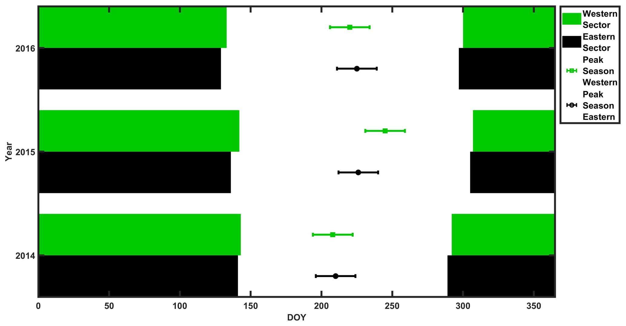
Figure 2 Time periods of frozen peat during the years 2014–2016 (green and black bars) and peak CH₄ emission season (dot with whiskers) for the western sector (green) and the eastern sector (black). (For peak season definition, see Sect. 3.2.)

3 Results

3.1 Environmental conditions and flux footprints

Winds from eastern and western sectors contributed to 50 % and 40 % to the daytime wind directions, respectively (Fig. 1). Northerly and southerly winds contributed to around 5 % each. In the nighttime, 51 % of wind was from the east and 32 % from the west. Additionally, 15 % of total wind came from the south during nighttime, probably as catabatic flow from higher mountain areas. The wind from the north was rare, around 2 % of all the cases.

The annual average peat temperature of the uppermost 50 cm of peat was systematically warmer in the eastern sector than in the western sector (Table 1; Fig. 3). However, the summertime peat temperature at the top 10 cm layer was warmer for the western sector (Fig. S5). The situation was the opposite during winter when the western sector down to 50 cm was colder than the eastern sector. During our investigation period (2014–2016), the peat temperatures from 30 to 50 cm below ground were colder in the western sector than those of the eastern sector, corresponding to the existence of the permafrost. Temperature differences, between both areas, at the same depth, were stable over the measurement years. The biggest difference was noticed at a depth of 30 cm. The temperatures at 30 and 50 cm depth were increasing during consecutive years.

Figure 3 Time series of daily mean values for western and eastern sectors for peat temperature (a, b), soil moisture (c, d), and water table level (e, f), where the shaded light blue area is the frozen period, when peat temperature at 10 cm was below 0 ^∘C (see Sect. 2.8 for a detailed description).

Table 1 Mean annual air and peat temperatures for the years 2014–2016 for eastern and western sectors.

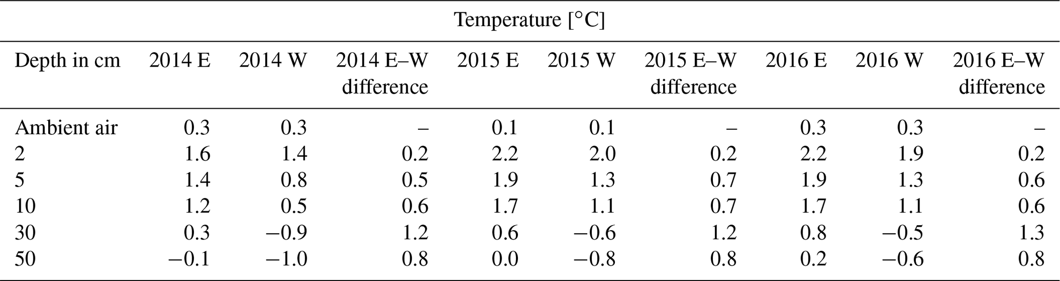
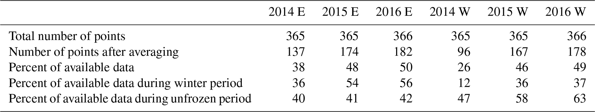
Table 2 The size of available daily datasets after gap-filling by daily averaging for each year and wind sector.

Both the WTL and SWC show 2014 to be slightly drier than 2015 and 2016, especially in the eastern sector. However, in the western sector the WTL was measured in an isolated wet patch, surrounded by drier palsa covering most of the area, and thus it is not representative of the dominant type of this area. The WTL in the eastern sector was more representative of the area of the footprint. The water table and soil moisture were higher for the eastern than the western sector during all years. The data show a distinctive step change at thaw and freeze, as the dielectricity of ice and liquid water differs. In the eastern sector, the soil was fully saturated for most of the unfrozen period during the years 2015–2016, while 2014 indicates lower water content levels. The western sector was never fully saturated at any time during the years 2014–2016.

Footprint and flux contribution of drier and wetter areas are presented in Fig. 4. The dry areas (yellow) contribute on average over all 3 years to more than 90 % of the fluxes measured from the western sector at the eddy covariance tower. In the eastern sector, the wetter (blue) and drier areas contribute almost equally to the fluxes. The contributions of the wet and dry areas to the fluxes in both sectors remained almost constant across the 3 study years.

Table 3 Gaps distribution over years and wind direction.

3.2 CH₄ fluxes

We analyzed the growing season data of each year and both wind sectors separately in regards to a possible diel cycle of CH₄ fluxes. This was done by normalizing each half-hourly flux by dividing it with the daily median from that day for the whole growing season (Rinne et al., 2007). This yielded a normalized diel cycle of CH₄ fluxes. Figure S6 shows slightly lower emission during midday hours. However, the difference is small compared to the short-term variation in the fluxes as indicated by the interquartile range. Thus, for the purpose of gap-filling this effect could be negligible in calculating daily averages. However, it is interesting to observe this type of diel cycle, with minima at daytime. It could be linked to the temperature cycle of the top peat layer. This could affect the methanotrophy, while the methanogenesis occurring at slightly deeper layers would be less affected. This would lead to higher methanotrophy at daytime and thus lower emission. It is possible to calculate CH₄ daily averages without gap-filling the diel cycle, similarly to, e.g., Rinne et al. (2007, 2018) and Jackowicz-Korczyński et al. (2010). We discarded daily averages with less than 10 flux data points from further analysis to ensure the reliability of the daily average fluxes. Uncertainties of daily averages were calculated as standard errors of the mean. The size of the available flux dataset, after gap-filling by daily averaging, is presented in Table 2. The gap distribution in the datasets for the different sectors and years is presented in Table 3.

Daily non-gap-filled CH₄ fluxes showed a characteristic annual cycle, with peak emissions in August (Fig. 5) and low but positive wintertime fluxes. Wilcoxon rank sum tests need data without autocorrelation. The autocorrelation in the data existed up to 8 d. Based on this we divided winter data with subsets where every ninth day was selected. We tested the difference of those subsets to zero with the Wilcoxon rank sum test. Winter fluxes were statistically different from zero (p<0.001, two-sided Wilcoxon rank sum test). Winter fluxes from the western and eastern sectors were also different from each other (p<0.001).

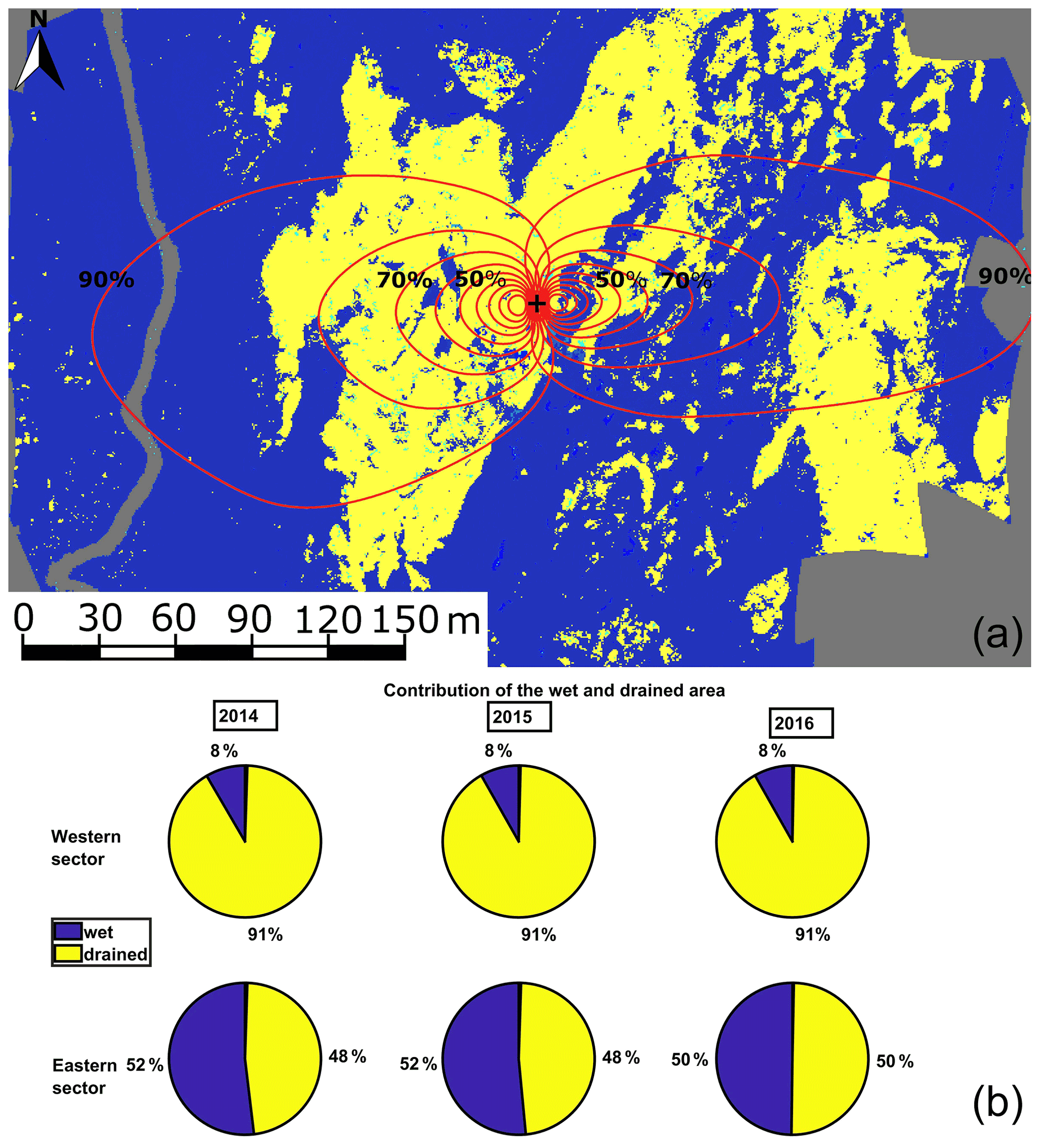
Figure 4 Footprint-weighted contribution of the wet and drained area at the SE-Sto tower (a) for the year 2014 and relative amounts of wetter areas (blue) and the drained palsa area (yellow) inside the 80 % area of influence of the footprints (b). The black cross is the location of the tower, and each red line indicates 10 % of the contribution from the source area to measured fluxes at the tower. The footprint climatology is almost identical for all study years; see bottom panel.

CH₄ fluxes, both from the western sector and the eastern sector, started increasing after snowmelt up to a maximum in August (Fig. 5). No major springtime emission burst or autumn freeze-in burst was observed in any of the years.

The middle day of the peak season of the CH₄ emission was defined as the maximum of the 14 d moving average. Two weeks forward and backward from the middle day was defined as the peak season, and emissions were estimated for that period in each year. The average emission during the peak seasons was 40 mg-C m⁻² d⁻¹ for the eastern sector and 19 mg-C m⁻² d⁻¹ for the western sector. Detailed emissions for all years are presented in Table 4. The peak season emissions were statistically different from each other (p<0.001). Wintertime fluxes were steadily declining as winter continued, and the lowest emissions were observed slightly before the spring thaw. Wintertime average emissions were 9 mg-C m⁻² d⁻¹ for the eastern sector and 6 mg-C m⁻² d⁻¹ for the western sector. Detailed emissions of winter periods are presented in Table 5.

Table 4 CH₄ emission during the peak season.

3.3 Factors controlling the CH₄ fluxes

In the eastern sector, the CH₄ flux correlated best with the peat temperature at 30 cm depth, and in the western sector it correlated best with the temperature at 10 cm depth. Using temperatures above the level of maximum correlation led to similar hysteresis-like behavior in CH₄ flux – temperature relations as presented by Chang et al. (2020), but using deeper temperatures led to inverse hysteresis compared to shallower temperatures (Fig. 6). The correlation matrix (Fig. S3) shows the importance of SWC in the CH₄ emissions, while WTL does not correlate significantly with CH₄ flux. Controlling factors were examined before and after temperature normalization of the CH₄ fluxes following Rinne et al. (2018) (Table 6) in order to avoid effect of cross-correlation between explanatory parameters.

Table 5 CH₄ emission during the winter period.

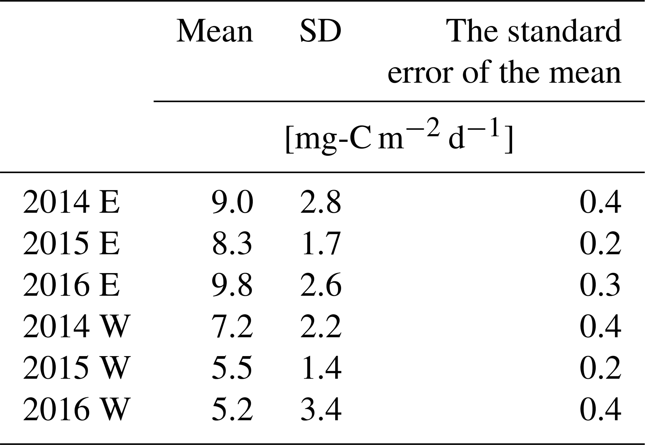
Table 6 Summary of controlling factors before and after temperature normalization.

The result from the GLM, showing the variables that contribute to the model, is presented in Table S2. The parameter that was selected first by all models was peat temperature at 10 cm depth for the western sector and at 30 cm depth for the eastern sector. For the eastern sector, the GLM algorithm selected SWC as the explanatory factor for CH₄ fluxes during all years as well as for the combined 3-year period. The GLMs created for the western sector did not have other explanatory factors besides the peat temperature that were selected in all years. However, two more explanatory factors, GPP and shortwave incoming radiation, appeared in the three time periods (years 2015 and 2016 and 3 years combined) for the western sector.

The eastern sector models had shortwave incoming radiation as the explanatory factor for the year 2015, the year 2016, and the combined 3-year period. A unique variable for this sector was the vapor pressure deficit, which was used in the models constructed for the years 2016 and combined 3-year period.

The year 2014 was characterized by a smaller number of parameters contributing to the models for both sectors compared to other years and combined 3-year models. Only peat temperature and SWC were explanatory variables for both sectors in this year. The years 2015 and 2016 and all 3 years combined have a longer list of parameters.

As the WTL data were available only during a short period of the year; they were not analyzed with the GLM. The WTL measurement in the western sector was not representative of the conditions for most of the sector; this parameter was not used for further analysis from this sector. The WTL was correlated with CH₄ fluxes for the eastern sector.

Based on the chosen explanatory variables it was noticed that the seasonal cycle could be explained by a lower number of parameters than the interannual variation.

3.4 Gap-filled annual cycles

Cumulative CH₄ emissions based on different gap-filling methods are presented in Fig. 7. All follow a similar annual curve, with a steeper increase in summer, but also relatively high wintertime contribution. Annual, wintertime, and unfrozen period emissions by all gap-filling methods, with their estimated uncertainties, are shown in Fig. 8. Emission estimation by each sector and data gap-filled by the different method are presented in Table S3. Average values from all models with their upper and lower limit and wintertime contribution to fluxes are demonstrated in Table 7.

Table 7 Average CH₄ annual emission based on all models with the upper and lower limit and contribution from the winter fluxes.

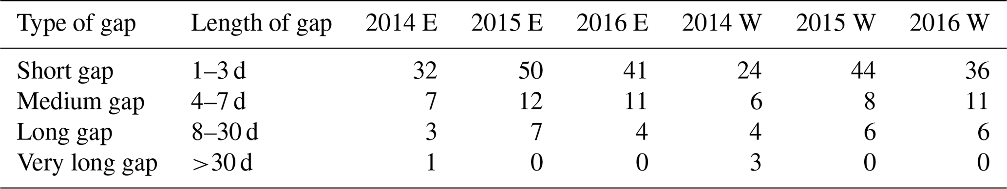
As can be seen in Table 3, the year 2014, with a larger difference between annual emissions calculated by different gap-filling methods, had very long gaps that were not present in other years. Also, the uncertainties in annual emission are the largest for the year 2014 for all gap-filling methods, reflecting the gap distribution.

The 3 years' averages of GPP and net ecosystem exchange (NEE) for two sectors are presented in Table 8. As comparison, data from lake and tall sedge fen areas at the Stordalen Mire complex, where permafrost was completely thawed, are also presented (Jammet et al., 2017). The fen has the highest percentage of carbon emitted as CH₄, as compared to the annual net CO₂ uptake. The eastern and the western sectors emitted less of the assimilated carbon as CH₄ compared to the completely thawed area. The uptake of carbon as CO₂ was also largest at the fen.

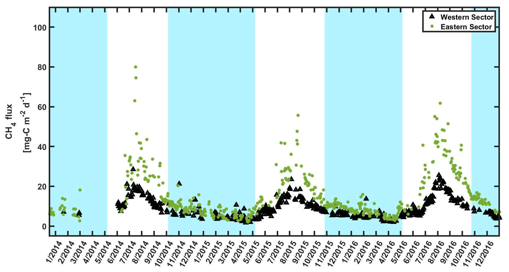
Figure 5 Time series for non-gap-filled CH₄ daily averaged fluxes for the western sector (green triangles) and the eastern sector (black dots), where the shaded light blue area is the frozen period when peat temperature at 10 cm was below 0 ^∘C (see Sect. 2.8 for a detailed description).

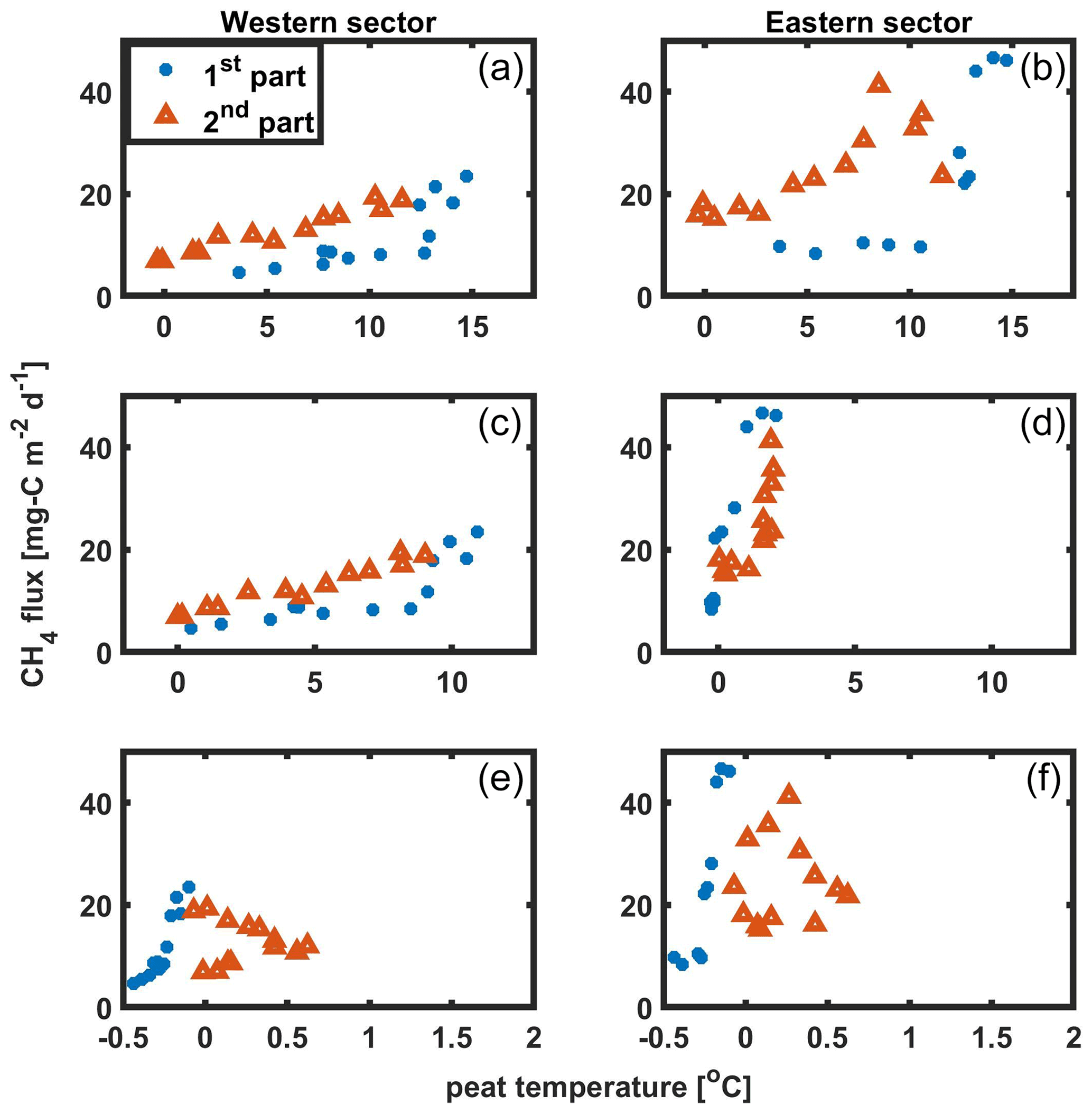
Figure 6 Weekly averages of CH₄ fluxes against the surface peat temperature (a, b), the depth with best correlation (c, d), and the deeper layer (e, f). Data were divided into the first part of the growing season (blue dots) before the maximum weekly emission and the second part of the growing season (orange triangles) after that.

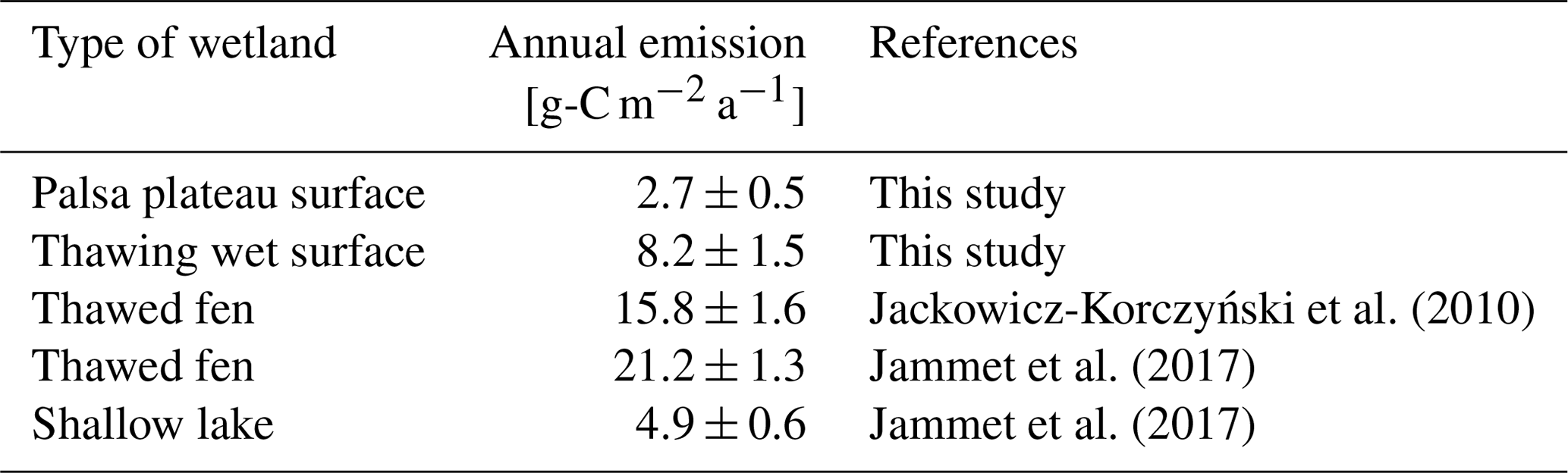
The 3 years' annual average CH₄ emissions of palsa and thawing surfaces, as calculated by Eqs. (1) and (2), are presented in Table 9. For comparison, average annual emissions from other major surface types, measured by EC technique, are shown as well. The emission from the tall graminoid fen, a third mire type common at Stordalen Mire, has been previously measured using the EC method by Jackowicz-Korczyński et al. (2010) and Jammet et al. (2017). In addition to these, the mire complex includes shallow lakes. Their annual CH₄ emission has been measured using the EC method by Jammet et al. (2017).

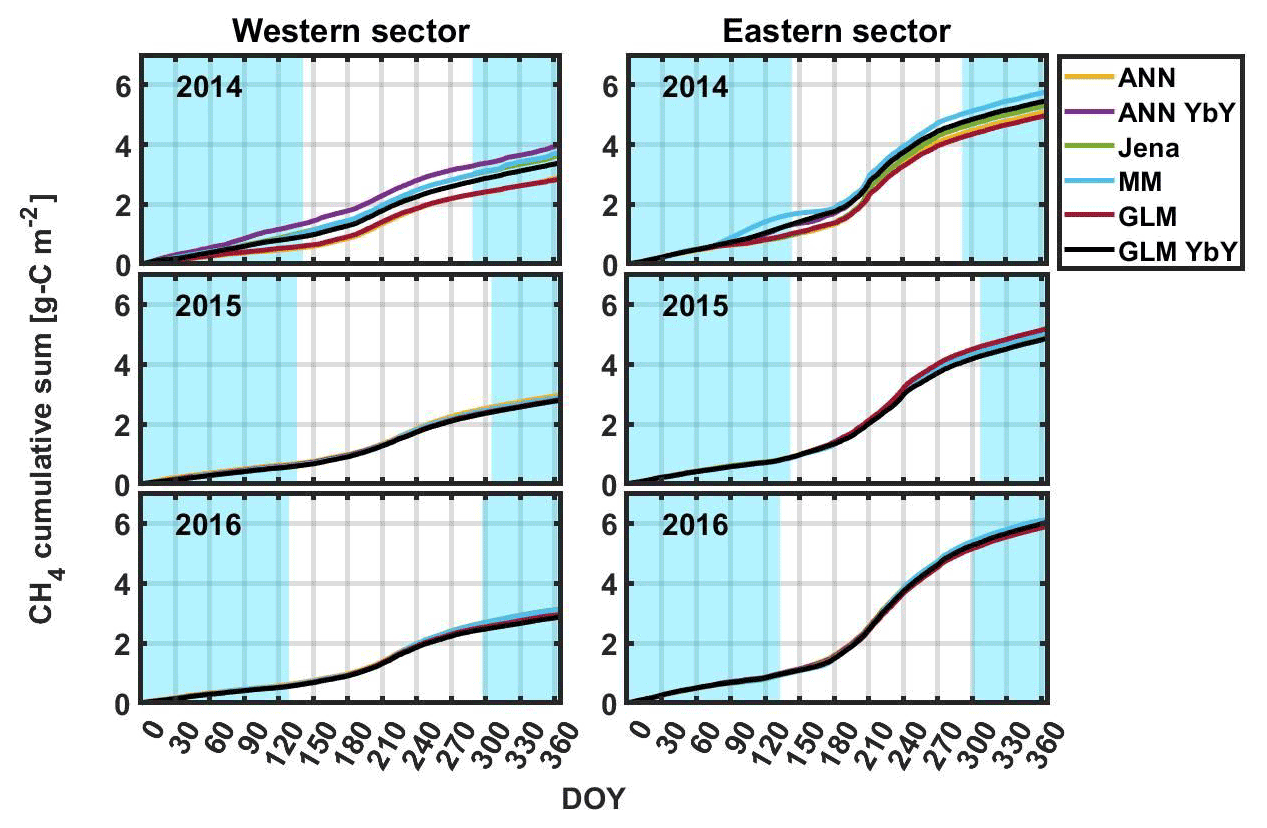
Figure 7 The cumulative sum of CH₄ fluxes for the years 2014–2016 for western and eastern sectors calculated with the different gap-filling methods. ANN – the artificial neural network for all years; ANN YbY – artificial neural network each year separately; Jena – Jena online gap-filling tool; MM – moving mean with 5 d moving window; GLM – the general linear model for all years; GLM YbY – the general linear model for each year separately. The shaded light blue area designates the frozen period when peat temperature at 10 cm was below 0 ^∘C (see Sect. 2.8 for a detailed description).

Figure 8 Comparison of cumulative sums of CH₄ fluxes for different gap-filling methods for the western sector (a, b, c) and eastern sector (d, e, f). ANN – the artificial neural network for all years; ANN YbY – artificial neural network each year separately; Jena – Jena online gap-filling tool; MM – moving mean with 5 d moving window; GLM – the general linear model for all years; GLM YbY – the general linear model for each year separately. Gray bars are for the annual sums, blue bars are for the frozen period sums, and green bars are for the unfrozen period (see Sect. 2.8 for a detailed description). Solid lines are the mean value from all models, and dashed lines are for the standard deviation range, with the same colors described above.

4 Discussion

4.1 Differences in controlling factors

According to the GLM, peat temperature and GPP were typically the first parameters selected by the algorithm to explain CH₄ fluxes. In the eastern sector, the CH₄ flux correlated best with the peat temperature at 30 cm depth, and in the western sector it correlated best with the peat temperature at 10 cm depth. Temperature as a controlling factor of CH₄ emission has been reported in many wetland studies (Christensen et al., 2003; Jackowicz-Korczyński et al., 2010; Bansal et al., 2016; Pugh et al., 2017; Rinne et al., 2007, 2018), in line with our findings. The correlation of CH₄ fluxes with the temperature at 5 cm depth was also higher than for 30 cm in the western sector. As the peat in the palsa is frozen at 30 cm depth for most of the growing season, the correlation between CH₄ fluxes and temperature at these depths is lower. Temperature correlation for the upper part, at 2 and 5 cm depth, shows a similar level of correlation as presented by Jackowicz-Korczyński et al. (2010). As they did not analyze correlation with the temperature at deeper peat, we cannot compare these results. The hysteresis-like behavior of the CH₄ flux – temperature relation is similar to that observed by Chang et al. (2020) when using temperatures measured above the depth of maximum correlation but inversed when using temperatures measured at deeper depths (Fig. 6). This is in line with at least part of the hysteresis-like behavior being due to the lag of seasonal temperature wave at the depth of CH₄ production compared to the timing of the temperature wave at shallower depth or air temperature.

Table 8 Average annual GPP, NEE, and CH₄ emission from the western and eastern sector in comparison to fen.

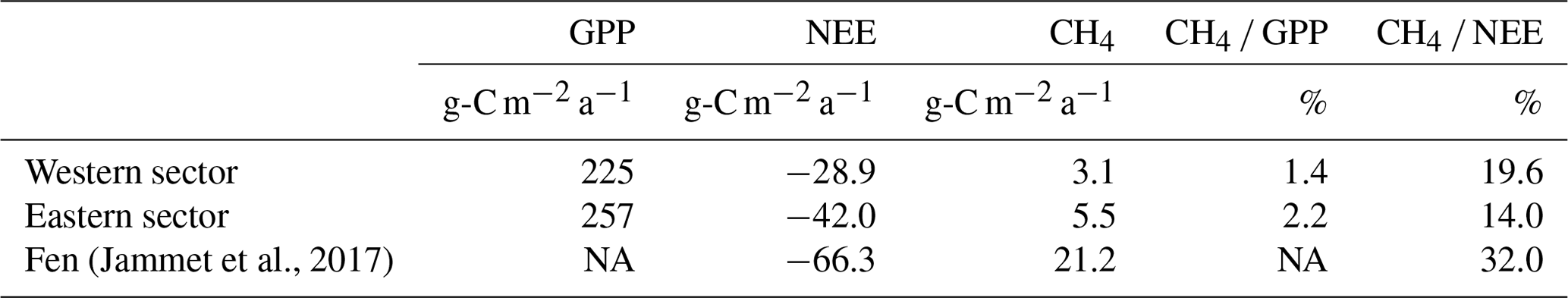
NA: not available.

GPP was indicated as a controlling factor for CH₄ emission from a boreal fen ecosystem by Rinne et al. (2018). In our study, the correlation matrix shows a significant correlation between daily average GPP and CH₄ flux at both sectors (Table S3). To disentangle the confounding effects of temperature and GPP, we used temperature-normalized CH₄ fluxes following Rinne et al. (2018), which revealed that the correlation between GPP and temperature-normalized CH₄ flux was not significant in most years (Table 6). Only the data from the eastern sector in the year 2016 show a significant correlation. Thus, it seems hard to disentangle the effects of temperature and GPP on CH₄ fluxes using this dataset. As our dataset consists of only 3 years, the analysis of interannual variations would not be a robust approach either.

Solar shortwave incoming radiation was selected as a controlling variable by six of eight GLM models (Table S3). This parameter has an indirect effect on CH₄ production via photosynthesis and subsequent substrate production. The maximum emission of CH₄ occurs later in the year than maximum radiation. This may be due to the CH₄ emission depending on the deeper peat temperature or seasonal cycle of available substrates, lagging behind the annual cycle of radiation (e.g., Rinne et al., 2018; Chang et al., 2020). The negative contribution of shortwave radiation in GLM can be due to the slight diel cycle of CH₄ emission, with the lowest values at daytime. Mechanistically we can think that the solar irradiance will heat the top of the peat layer, thus leading to increased methanotrophy at daytime (see discussion above on diel cycle). This can lead to a situation where the methanotrophy is higher in sunny days with warm surface and lower in cloudy days. The role of photosynthesis for the substrate supply of methanogenesis is likely to act in the seasonal timescale, where its effect can be masked by the strong correlation between peat temperature and CH₄ emission. The highest correlation of CH₄ flux and radiation was observed in 2014, but GLM did not select radiation as an explanatory factor for this year. Other years and the whole period show a much lower correlation.

CH₄ fluxes from wetlands have been shown to depend on WTL in many studies (e.g., Bubier et al., 2005; Turetsky et al., 2014; Rinne et al., 2020). However, in a number of studies, the CH₄ fluxes have shown to be relatively insensitive to the small variation, without strong extreme conditions in the WTL (Rinne et al., 2007, 2018, Jackowicz-Korczyński et al., 2010). In the eastern sector, CH₄ flux and WTL were correlated for the years 2014 and 2016. However, after normalization of CH₄ fluxes with their temperature dependence following Rinne et al. (2007), correlations were mostly not significant (Table 6). This is similar to conclusions drawn by, e.g., Rinne et al. (2007, 2018) and Jackowicz-Korczyński et al. (2010).

Instead of WTL, we used SWC as a possible controlling factor for the CH₄ emission from the western sector. Sturtevant et al. (2012) also reported SWC as a controlling factor in autumn. SWC shows correlation on a significant level before and after normalization for 3 years for the western sectors (Table 6).

The GLM algorithm selected SWC as one of the explaining factors while constructing the GLM for the eastern sector for the whole measurement season. It was chosen by models built for 3 years together and each year separately. R and p values are presented in Table 6. A reduction of R and increase in p value after temperature normalization is similar to previous parameters. The correlation of CH₄ emission with SWC stays on a significant level only in the year 2016.

Table 9 Annual CH₄ emission from different components of the Stordalen Mire complex from EC studies.

4.2 Gap-filling methods

In general, the gap-filled annual CH₄ emissions were within their estimated uncertainty from each other, apart from the year 2014. The results of different gap-filling methods were affected by the different gap distributions and lengths in different years and the two wind sectors. Thus, below we discuss the method performance separately for the year 2014 and the 2 other years.

The dataset from the eastern sector was gap-filled with higher confidence than for the western sector in 2014. The data from the eastern sector contain fewer very long gaps (more than 30 d) and fewer long gaps (more than 8 but less than 30 d). The method which was most affected by long gaps was the moving mean approach, indicating that this method should not be used for datasets with very long gaps. The ANN and the GLM gap-filling methods based on the whole dataset estimated lower annual emission than mean emission from all methods. For 2 years without very long gaps (2015 and 2016), the Jena gap-filling tool was assumed to be a baseline method, as it is commonly used for gap-filling of especially CO₂ fluxes. It is independent of the user choices, as the ecosystem variables required have been chosen by the developers. However, as this gap-filling tool has been developed for CO₂, not all the variables are necessarily relevant for the gap-filling of the CH₄ time series. Furthermore, the Jena gap-filling tool works in a half-hourly resolution to resolve the diel variation in CO₂ fluxes. As the sub-daily variation in CH₄ fluxes is largely random noise in many mires (Rinne et al., 2007, 2018; Jackowicz-Korczyński et al., 2010), developing a similar tool working at daily time step for CH₄, and with tailored parameter set for CH₄, would be useful.

The moving mean approach resulted in annual fluxes within the range of standard deviation from the Jena gap-filling tool. Daily values probably vary less than values obtained by the Jena tool because moving means smooth the data. Additional advantages of this method are low input requirements, as no auxiliary data are needed.

Annual estimates of CH₄ emission, based on the gap-filling with algorithms developed for the whole dataset, could be biased when the ecosystem is changing fast between the years and functional dependencies on environmental parameters change. The annual CH₄ emissions by ANN, based on the whole dataset and based on 1-year data, agree within the standard deviation for the years 2015 and 2016. Both of them are also in agreement with the baseline method within the standard deviation.

The feasibility of GLM is similar to ANN. The GLM model built on the whole dataset is sensitive to rapid changes in ecosystem functioning and the number of gaps each year. A year with more gaps has a lower influence on the model, similarly to the ANN. However, annual CH₄ emissions derived using GLMs, based on each year separately or the whole dataset, agree with one another and with the baseline model within the standard deviation. GLM required more preparation than ANN. Before developing the GLMs, highly correlated parameters need to be determined. The selection of relevant variables is crucial for the correct performance of that algorithm, and the selection influences model output and model uncertainties.

According to the analysis with artificial gaps, the 35 d artificial gap did not change annual sums significantly for any gap-filling method. The 80 d artificial gap created a significant difference for the eastern sector in the year 2015 for ANN YbY and 2016 for ANN (Fig. S7). The unfrozen period did not show significant differences between annual sums for any method. The wintertime period was statistically different for the year 2015 for ANN YbY. The results with the 80 d gap had higher uncertainties than the results with a 35 d gap. The existence of gaps in the winter period did not have a significant impact on the unfrozen period fluxes.

All presented methods show similar CH₄ emissions. Choosing one of them as the most appropriate is not obvious, because all of them show both advantages and disadvantages. The method that required the least amount of preparation before use and that was thus the fastest to apply is the moving mean. It can be used for short gaps with good results and does not need additional measured variables to work properly. The ANN method requires less preparation than other methods, i.e., following the template or choosing the correct variables, and it gives similar results. It could be recommended as a gap-filling method suitable for different sites due to unique construction of the ANN for each place.

4.3 Winter fluxes

The winter fluxes from both sectors were positive, which is in line with observations by, e.g., Rinne et al. (2007, 2018, 2020) and Jammet et al. (2017) of wintertime CH₄ emissions from frozen northern mires. Winter emission and potential spring thaw bursts of CH₄ can be mechanistically connected (Taylor et al., 2018), while degassing of CH₄ during the winter is likely to lead to smaller or no thaw bursts of CH₄. Thus, EC studies on the seasonal cycle of CH₄ emissions from other seasonally frozen mire ecosystems have shown minor or no thaw emission pulse (Rinne et al., 2007, 2018; Mikhaylov et al., 2015). On the contrary, many studies show spring thaw emissions from shallow lakes (Raz-Yaseef et al., 2017; Jammet et al., 2015, 2017). In lakes, winter fluxes can be blocked by a solid ice layer, leading to the buildup of CH₄ below ice during the frozen period (Jammet et al., 2017). On mires, however, the ice cover is not as solid as in lakes but more porous due to peat and plants within the ice. Therefore, the diffusion during the frozen period is considerably faster than through lake ice. Furthermore, Song et al. (2012) showed that spring burst events could occur at a very small scale and are very short in duration (e.g., 2 h). Small-scale events show a lower influence on EC measurements because the method averages over a larger area. Moreover, if the small-scale short-duration event does not happen in the EC footprint, e.g., due to wind direction, it will be missed.

We did not observe an autumn freeze-in burst in our data from either sector at Stordalen Mire. These events have been observed at a high-Arctic tundra site (Mastepanov et al., 2013), though not every year. Mastepanov et al. (2008) suggested that freeze-in bursts of CH₄ could be observed only in the Arctic with continuous permafrost and not in a subarctic area with discontinuous or sporadic permafrost. The phenomenon is assumed to be connected to the expansion of water upon freezing, causing air bubbles to be mechanically pushed out of the freezing soil.

4.4 Different permafrost status and CH₄ emissions

Stordalen Mire is a complex mire system, with at least three different main wetland surface types and different permafrost status within a distance of a few hundred meters. The permafrost palsa development and thaw depend both on temperature and snow cover, and it is partly self-regulating via the effect of microtopography on local snow depth (Johansson et al., 2006). Due to the recently increasing temperatures, the thaw processes are currently likely to dominate over palsa growth. CH₄ emission from the different microforms in mire systems depends on the hydrological and nutrient status and temperature which affect, e.g., plant and microbial communities.

The carbon emitted as the CH₄ fluxes from the eastern and western sector is on a similar level to the Siikaneva fen (Rinne et al., 2018). In comparison to the other fen sites reviewed by Rinne et al. (2018), the ratio of CH₄ to NEE at Stordalen Mire is higher. The reason behind this could be the shorter growing season and thus lower CO₂ fluxes.

The average annual CH₄ emissions from different surfaces (Table 9) show that the palsas have the lowest annual CH₄ emissions, followed by a lake. The fully thawed fen, dominated by tall graminoids, has very high annual CH₄ emissions and the highest of the mire complex, surpassing, e.g., many boreal poor fens (Nilsson et al., 2008; Rinne et al., 2018). The thawing surfaces common in the eastern footprint of the tower have annual CH₄ emissions between palsas and tall sedge fen. The three surface types studied here and previously by Jackowicz-Korczyński et al. (2010) and Jammet et al. (2017) can be seen as forming a thaw gradient in this subarctic environment. The globally rising temperature is likely to lead to continuing permafrost thaw in this kind of ecosystem and increased CH₄ emissions.

5 Conclusions

At our study site, eddy covariance fluxes were measured for two different subarctic mire areas, one dominated by palsa plateaus and the other a mixture of palsas and thawing wet surfaces. The measurements revealed clear differences in their annual CH₄ emissions, with the area dominated by palsas emitting less. The annual emission from a thawing surface (8.2 g-C m⁻² a⁻¹) was nearly 3 times higher than from palsa surfaces (2.7 g-C m⁻² a⁻¹) but only half of the emission previously reported from fully thawed tall graminoid fen. Areas measured in this study had similar seasonal cycles of emission, with maxima appearing in August and lower but significant fluxes in winter. The seasonal cycles were furthermore characterized by a fast increase in spring (average 0.21 mg-C m⁻² d⁻² for the western sector and 0.68 mg-C m⁻² d⁻² for the eastern sector) and a less rapid decrease in fall (average −0.16 mg-C m⁻² d⁻² for the western sector and −0.37 mg-C m⁻² d⁻² for the eastern sector), without any obvious burst events during spring thaw or autumn freeze-in. The wintertime period (from January to mid-May and from late-October to December) contributed with 27 %–45 % to the annual emission.

According to the correlation matrix and GLM analysis, CH₄ emissions from the western and eastern sectors were partly controlled by different factors. As in most studies on CH₄ emission from wetlands, peat temperature was the most important factor explaining the emission. The relation of CH₄ flux with peat temperature at shallower depths showed similar hysteresis-like behavior than observed by Chang et al. (2020) but inverse behavior with temperature at deeper peat. We showed that the existence and direction of hysteresis-like behavior can depend on which depth the temperature is measured at.

The correlation of CH₄ emission and WTL in the eastern sector was not significant, but in the western sector, the SWC did appear to control the emission.

The estimation of annual CH₄ emission was based on gap-filling with four different methods. All methods resulted in similar annual fluxes, especially for the 2 years with just relatively short gaps (less than 8 d). The performance of the methods was also dependent on the gap distribution. Long gaps (more than 8 d) were the most problematic to be reconstructed by any of the methods. The average annual emission from the western sector was 3.1 g-C m⁻² a⁻¹, and from the eastern sector it was 5.5 g-C m⁻² a⁻¹. Both were substantially lower than those obtained from a tall graminoid fen at the same mire system.

Based on the presented results, further studies should focus on winter fluxes, which are important in the northern, low-emission wetlands with discontinuous permafrost. There is still a lack of understanding of the processes behind those emissions. Also, the origin of wintertime CH₄ emission is somewhat unknown. On the one hand, CH₄ can be produced during the winter period; on the other hand, CH₄ can also be produced during the growing season, remain stored in the peat, and then be slowly released during the frozen period. These processes could possibly explain the hysteresis-like behavior of CH₄ emissions.