the Creative Commons Attribution 4.0 License.
the Creative Commons Attribution 4.0 License.
 | 01 Dec 2021
Simultaneous assessment of oxygen- and nitrate-based net community production in a temperate shelf sea from a single ocean glider
Naomi Greenwood
Antony Birchill
Alexander Beaton
Matthew Palmer
Jan Kaiser
The continental shelf seas are important at a global scale for ecosystem services. These highly dynamic regions are under a wide range of stresses, and as such future management requires appropriate monitoring measures. A key metric to understanding and predicting future change are the rates of biological production. We present here the use of an autonomous underwater glider with an oxygen (O2) and a wet-chemical microfluidic total oxidised nitrogen () sensor during a spring bloom as part of a 2019 pilot autonomous shelf sea monitoring study. We find exceptionally high rates of net community production using both O2 and water column inventory changes, corrected for air–sea gas exchange in case of O2. We compare these rates with 2007 and 2008 mooring observations finding similar rates of consumption. With these complementary methods we determine the O2:N amount ratio of the newly produced organic matter (7.8 ± 0.4) and the overall O2:N ratio for the total water column (5.7 ± 0.4). The former is close to the canonical Redfield O2:N ratio of 8.6 ± 1.0, whereas the latter may be explained by a combination of new organic matter production and preferential remineralisation of more reduced organic matter at a higher O2:N ratio below the euphotic zone.
- Article
(1616 KB) - Full-text XML
- BibTeX
- EndNote


The coastal shelf seas are a vitally important human resource for numerous ecosystem services, including food, carbon storage, biodiversity, energy, and livelihoods (Halpern et al., 2015). They have a disproportionately large impact, relative to their surface area, on global carbon cycling (Thomas, 2004) as shelf seas provide 10 %–30 % of all marine primary production while comprising less than 10 % of the ocean surface (Harris et al., 2014; Sharples et al., 2019). Given their global role in carbon cycling, understanding the mechanisms driving primary production is vital for predicting how shelf systems will respond to and influence climate change (Palevsky et al., 2013; Legge et al., 2020).
The North Sea is a semi-enclosed region of the northwest European continental shelf between the island of Great Britain in the west and Norway, Denmark, Germany, and the Netherlands in the east and south. The northern boundary is facing the North Atlantic. It can be divided into two energetically distinct regimes: a seasonally stratifying northern part and a fully mixed southern and coastal part (Emeis et al., 2015). The shallower fully mixed region is believed to act as a net sink for CO2 during the spring bloom periods and a source of CO2 during the rest of the year (Emeis et al., 2015; Hull et al., 2016). Thomas et al. (2005) suggest that the seasonally stratified regions are a sink for carbon throughout the year. A more recent synthesis of Kitidis et al. (2019) indicates that the seasonally stratified regions were a source of CO2 during December and January in 2015.
The North Sea is one of the most well-studied marine environments. However, despite the availability of large volumes of data, making robust statements on the long-term changes, natural variability, or predicted process responses to external forcing continues to be challenging (Emeis et al., 2015). As is typical for shelf regions, the North Sea displays high temporal and spatial variability, which makes the analysis of trends more challenging compared with the open ocean (Bozec et al., 2006; Bauer et al., 2013). At present, resolving the nutrient and oxygen dynamics in shelf sea regions remains a challenge for numerical biogeochemical models (Bauer et al., 2013; Emeis et al., 2015). Further development of model parametrisations for these processes, in addition to validation of the model outputs over appropriate spatial and temporal scales, is required.
The North Sea is changing, and the processes controlling the carbon, oxygen, and nutrient dynamics are highly complex and interconnected (Wakelin et al., 2020). Key among those processes is marine production. Estimates of net community production (NCP) can quantify the uptake of CO2 from the atmosphere into the sea (Alkire et al., 2012; Hull et al., 2016; Plant et al., 2016). Changes to community production can affect how organic material is exported to and respired within the non-ventilated waters below the thermocline (Große et al., 2016). NCP is therefore a useful metric for understanding carbon cycling and an important control on bottom water oxygen concentration.
1.1 The Dogger Bank
The Dogger Bank is a large sandbank within the central North Sea (Fig. 1). Comprising predominantly fine sand and mud, this bank rises 20 m above the surrounding sea floor and is 15 m below sea level in its shallowest parts. The Dogger Bank sits south of a tidal front, which is located in an arc across the central North Sea from Yorkshire in the United Kingdom to the Frisian coast in the Netherlands. This hydrological divide separates well-mixed waters to the south from the seasonally stratified waters of the central North Sea to the north (Emeis et al., 2015). The combination of tidal, wind, and buoyancy forcing tends to develop a general anti-clockwise circulation within the North Sea (Mathis et al., 2015). Variability in the circulation is determined mainly by variation in local winds, which are predominantly from the west. Tidal forcings are dominated by the M2 constituent, with mean tidal excursion in the region of 1.5 km (Fig. 1). Prevailing currents move from the west along the tidal front towards the Dutch coast. These currents are supplied with water from the Scottish coastal current, itself primarily fed from the North Atlantic inflow through the Orkney–Shetland gap (Hill et al., 2008). The Dogger Bank experiences minimal riverine influence, such that maximal nutrient concentrations typically reflect those of the in-flowing Atlantic waters (Greenwood et al., 2010). The changes in N:P ratio observed in more coastal regions of the North Sea are not seen at Dogger Bank, and nitrogen remains the primary limiting nutrient (Burson et al., 2016).
The shallow waters above Dogger Bank are not seasonally stratified as wind stress and tidal currents regularly homogenise the shallowest areas, which replenishes nutrients into the photic zone throughout the year (Riegman et al., 1990). In this paper we focus on the region north of the Dogger Bank where mixed waters converge with the seasonally thermally stratified waters. The exchange of nutrients and phytoplankton at this transition promotes enhanced primary production along the northern edge of the bank, which acts as a hotspot for marine life and supports several important fisheries (Plumeridge and Roberts, 2017). Since 2017, the bank has been designated as a Special Area of Conservation (SAC) by the UK government, signifying it as a region containing habitats and species which are considered most in need of conservation and legal protection. The area on and around Dogger Bank is thought to exhibit year-round phytoplankton production (Nielsen et al., 1993). Due to the shallow depth of Dogger Bank, the spring phytoplankton bloom can be initiated there months before stratification triggers the bloom within the more northern stratified regions of the North Sea (Nielsen et al., 1993). The region north of Dogger Bank typically sees a spring phytoplankton bloom commencing at the start of April.
1.2 The AlterEco project
The glider-based oxygen and total oxidised nitrogen () concentration measurements presented within this paper form part of the larger AlterEco (“An alternative framework to assess marine ecosystem functioning in shelf seas”; https://altereco.ac.uk, last access: 29 September 2021) project. AlterEco is a pilot study of a novel monitoring framework to deliver improved spatiotemporal understanding of key shelf sea ecosystem drivers though the use of autonomous systems, primarily underwater gliders, as part of the Marine Integrated Autonomous Observing Systems programme of the Natural Environment Research Council (NERC). Buoyancy gliders are capable of directed, long-term continuous monitoring over a variable spatial area while covering the full water column within a shelf sea (Alkire et al., 2012; Wihsgott et al., 2019). Gliders have previously been fitted with UV-fluorescence-based sensors (Johnson et al., 2006). In the central North Sea potentially low concentrations of together with interferences from organic matter are a challenge for these instruments, which are typically more suitable for observing high concentrations in non-optically complex waters. Recent advances in wet-chemical microfluidic instruments present an opportunity to gather high-resolution and high-quality glider-based measurements. We use these to resolve the and oxygen fluxes and determine the net community production associated with the spring bloom simultaneously with two complementary methods.
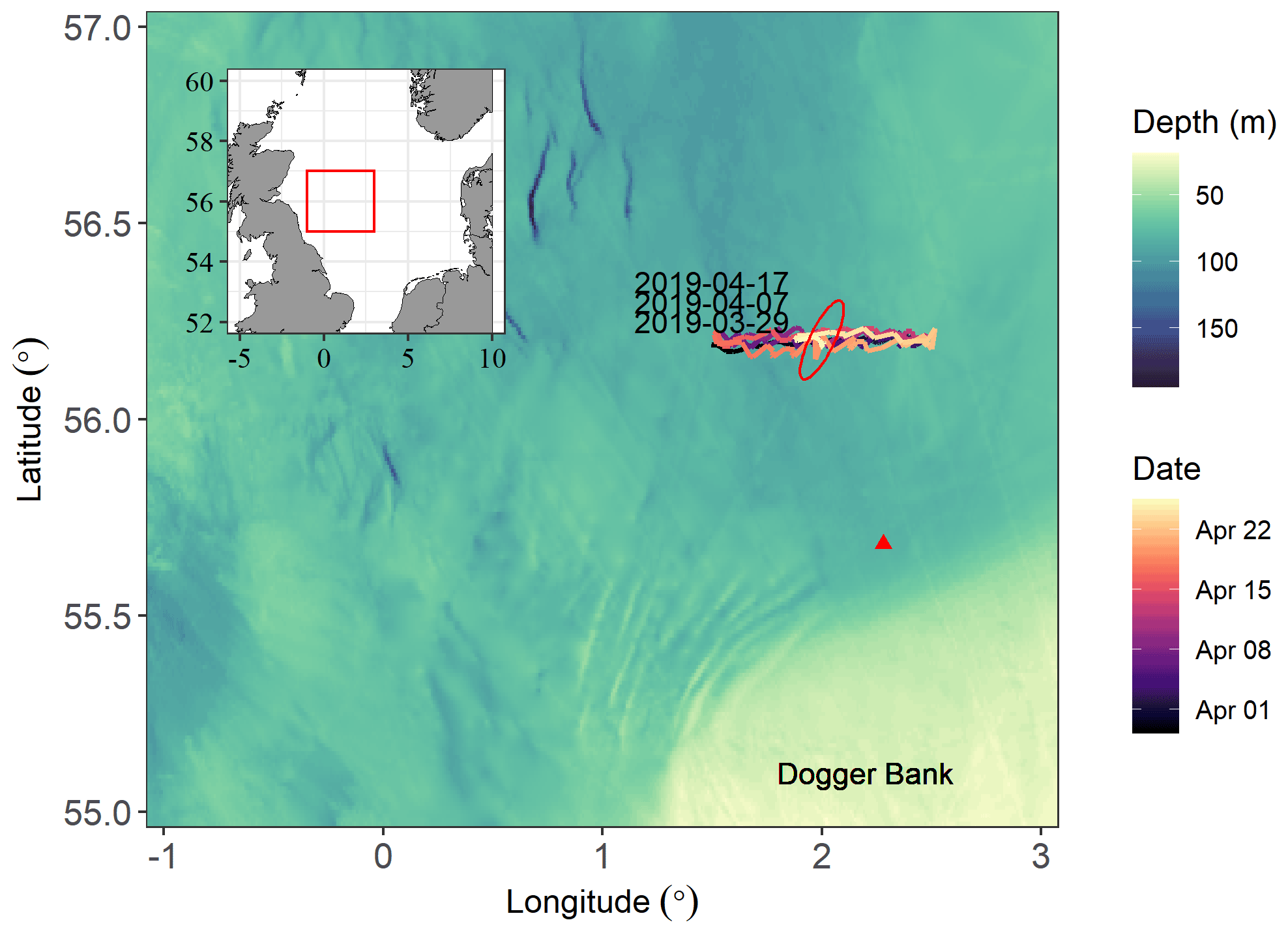
Figure 1Seaglider path for the AlterEco AE7 2019 mission and the surrounding study area. Timestamps indicate when the glider returned to the western side of the transect. Mean tidal ellipse shown in red (not to scale). Red triangle marks the location of the Centre for Environment, Fisheries and Aquaculture Science (Cefas) North Dogger SmartBuoy, present between 2007 and 2008. Bathymetry data from GEBCO (2019) on a 15 arcsec grid.
2.1 Study area
Observations were made along an east–west transect (Fig. 1) north of the Dogger Bank between 29 March and 25 April 2019 with an underwater glider (Seaglider sg602 “Scapa”). This period was the seventh group of AlterEco glider deployments and is therefore referred to by the mission code “AE7”. The Seaglider took 5 d to move from one end of the transect to the other and completed six transits. The glider was fitted with a standard non-pumped Seabird CT sail, an Aanderaa 4831 oxygen optode (Bittig et al., 2018), and a National Oceanographic Centre (NOC) lab-on-a-chip (LoC) microfluidic analyser (Beaton et al., 2012; Vincent et al., 2018).
The Seaglider conductivity, temperature (CT), and oxygen data were processed and quality-assured using the University of East Anglia (UEA) Seaglider toolbox (Queste, 2013). This comprised optimising the Seaglider flight parameters to determine speed though water, which was used to apply a cell thermal mass correction for the CT sensor. This is an iterative process as determining glider flight requires determining the water density, which is calculated from the measured salinity (Garau et al., 2011). Some salinity spikes still persist after performing the cell thermal mass correction due to strong vertical temperature gradients towards the end of the deployment (>0.8 ∘C m−1); these were manually quality-flagged (marked as bad) on a per-dive basis and not used in the analysis. As the Seaglider CT sensor relies on the forward movement of the vehicle to push water through the measurement cell, salinity and temperature values were also removed from the analysis where the glider speed was considered too slow to provide adequate flow through the cell (<0.1 m s−1).
2.2 NOx− observations
The LoC sensor is a miniaturised wet-chemical colorimetric analyser offering high-precision in situ total oxidised nitrogen measurement (Beaton et al., 2012). The analyser takes approximately 20 s to collect a sample and a further 7.5 min to perform an analysis. The concentration of the on-board artificial seawater nutrient standard was determined by laboratory continuous gas segmented flow analysis (Beaton et al., 2012; Vincent et al., 2018). Accuracy was determined with reference to two autoclaved natural seawater standards (KANSO Co. LTD, Japan) and summarised in Table A1. values below the limit of detection are treated as 0 mmol m−3 in our calculations. The limit of detection is 0.025 mmol m−3. Vincent et al. (2018) demonstrated excellent stability and agreement between data-generated LoC analysers deployed on an ocean glider and samples simultaneously collected by traditional shipboard techniques and analysed via standard gas segmented flow analysis. This Celtic Sea study region of Vincent et al. (2018) represents a similar shelf sea environment which exhibits a similar range of concentrations to the North Sea.
As the maximum depth along the AlterEco transect is less than 85 m, the glider was configured to perform periodic loiter dives to enable multiple samples to be collected and so maximise the vertical resolution of the samples (Vincent et al., 2018). With the standard Seaglider flight mode the glider pitch and buoyancy are adjusted to maintain a uniform speed during both the descent and ascent phase. A loiter dive consists of a standard descent phase, during which a blank and standard measurement are performed, followed by a deliberately slow ascent which provides time for the sensor to take more samples (n between 3 and 14). Along the transect standard dives took 30 ± 3 min, while loiter dives took 110 ± 5 min. The reduced speed of the glider during loiter ascent results in inadequate flushing of the CT cell, with impaired salinity data quality. We therefore extrapolate the salinity from the descent to the ascent data assuming the same pressure–salinity relationship.
Photosynthetic fixation of atmospheric carbon into new organic material by phytoplankton is associated with a corresponding consumption of inorganic nutrients (Anderson and Sarmiento, 1994). Where is the main source of nitrogen, the uptake represents net community production () (Plant et al., 2016). As the number and position in the water column of the samples is variable, the inventories are calculated on a per-dive basis after linear interpolation onto a 1 m vertical grid, the sum of which is then calculated to provide a full water column inventory. The standard uncertainty in the inventory is calculated from the squared sum of the relative concentration uncertainties (± 0.13 %) and a 0.5 m uncertainty in water column height. We exclude three dives where we are unable to calculate a full water column inventory as either the vertical spacing between samples near the thermocline was too large (>10 m) or samples are unavailable from each of the three vertical layers (Fig. 2d). For direct comparison with the Vincent et al. (2018) central Celtic Sea study we also calculate drawdown within the upper section of the water column down to a 40 m depth. This coincides with the mean euphotic depth for our study region in April 2018 as observed by another AlterEco Seaglider ( m) (Hull and Kaiser, 2020). The euphotic zone depth is defined as the depth to which photosynthetically active radiation (PAR) falls to 1 % of the level measured at the surface.
2.3 O2 observations
During typical (non-loiter) dives the Seaglider's vertical speed was typically 0.1 m s−1, and the oxygen sampling period was 10 s. The optode was multi-point-calibrated (10 concentrations at 4 temperatures each, 40 points total) by Aanderaa in January 2019 and referenced to in situ Winkler titrations taken during deployment and recovery. We adopted the recommendation of Bittig et al. (2018) that in the absence of reference data spanning a wide range of oxygen concentrations a correction factor (gain) should be applied to calibrate the oxygen concentration, i.e. where , a=0 and b>1. This is in contrast to an offset, a combination of offset and factor, or a correction applied to the raw phase reading of the optode (Uchida et al., 2008). Reference to the discrete samples remained challenging as the deployment location was within a region of significant horizontal heterogeneity. The reference location was as close as possible to the study region but was legally constrained to within 60 nm from the coast due to the small coastal vessel used. Drift in the optode response to oxygen was assumed to be linear with respect to time and corrected based on the deployment and recovery samples (−0.025 % d−1) (Tengberg and Hovdenes, 2014; Bittig et al., 2018).
Biological oxygen production can also be used as a proxy for net community production (J(O2)), with a net production of oxygen indicative of a net autotrophic system (Alkire et al., 2014; Hull et al., 2016). We implement an oxygen mass balance model to separate the physically and biologically driven components of the observed oxygen inventory changes. As with the mass balance we calculate values for the euphotic zone (zI=40 m) and the full water column (zI=82 m). Full details of this model and its implementation are found in the Appendix Sect. A1.
2.4 Supporting data
Local wind speed and atmospheric pressure were obtained from ECMWF ERA5 reanalysis (Copernicus, 2018). These hourly data were matched to the spatiotemporally closest Seaglider dive. For ocean currents at the AlterEco site we use the UK Met Office Operational Suite Atlantic Margin Model (FOAM) 1.5 km configuration (run 18 May 2020) (Graham et al., 2018). Bathymetry was taken from GEBCO (2019) on a 15 arcsec grid. Between 2007 and 2008 an autonomous monitoring buoy (SmartBuoy; Greenwood, 2016) was located to the south of the Seaglider transect (Fig. 1). This platform collected near-surface 0.5 and mid-water (25 m) O2 concentration measurements using similar sensors to the Seaglider and presents an opportunity for determining interannual variability. Full details of this platform are provided in the Appendix A2.
3.1 Overview
The Seaglider reached the transect on 29 March 2019 at 04:00 UTC (Fig. 1), at which point the water column was weakly stratified, with the base of the surface mixed layer at 30 m and a 0.03 ∘C temperature difference across the thermocline (Fig. 2b). Horizontal heterogeneity was seen across the 64 km transect with the eastern end persistently cooler (0.5 to 1 ∘C) than the western end. Figure 2a, b, and d demonstrate this gradient to be non-linear and differing between the upper and lower layers. This can also be observed in the salinity time series where a more saline region was seen between 1.8 and 2.4∘ E, with fresher water at both ends of the transect. While the bottom mixed layer (BML) oxygen concentrations on the eastern side of the transect were 3 to 5 mmol m−3 higher than elsewhere, the saturation is similar throughout, which indicates that the increased oxygen concentration was mostly due to higher solubility at lower temperatures.
Mean wind speed was 6.7 m s−1, with a peak of 12.6 m s−1. Modelled residual surface currents were to the north-west (counter to the typical annual residual flow), with surface waters moving into the transect area from across the bank. Surface mean current speed was 0.17 m s−1 with a maximum of 0.39 m s−1. We calculate a cumulative total surface advection at the centre of the transect of 52 km over the 27 d occupation of the transect, with a mean residual flow of 0.02 m s−1. Tidal advection was typically 5 km over 25 h. The tidal ellipse is shown in Fig. 1. Bottom water residual flow was small (0.004 m s−1), with a period of flow to the north until 12 April 2019 and then to the south. As a result, bottom water is estimated to have moved less than 9 km while the glider was on the transect. Given the 10 d transit time for the glider to return to the same end of the transect, surface water may have been advected 19 km during that time.

Figure 2Seaglider location along the transect (a), with associated temperature (b) and mixed layer depth (green line), oxygen concentration (c), salinity (d), and nitrate (e) profiles. Temperature, oxygen, and salinity data are vertically aggregated into 3 m bins for each dive. Dark-grey areas indicate data removed though quality control procedures. Samples which are excluded from the inventory are signified with a green triangle marker.
There is disagreement regarding the importance of horizontal advection to mass-balance-based estimates in this region (Queste et al., 2013; Rovelli et al., 2016; Große et al., 2016). Given the slow speed of the glider relative to the rates of change in the inventories and uncertainties due to the lack of observations to the north and south, it is not possible to fully resolve any persistent or evolving horizontal (or O2) gradient for a 1D mass balance. The tidally driven advection of the glider is largely inconsequential to the data it collects as the glider drifts with the ebb and flow of the tidal currents. Using the modelled residual surface currents and taking the difference in near-surface concentrations observed across the first transect as indicative of the horizontal gradient ( mmol m−4) suggests a horizontal advective flux of 0.05 mmol m−2 d−1, which can be neglected for the purposes of the present paper. The effect for O2 is similarly small.
The thickness of the thermocline varies substantially over the deployment, ranging from 6 to 53 m (see Figs. 2b and A1). Vertical fluxes across the thermocline are only relevant to the mass balance when the base of the thermocline is below the 40 m integration depth (seen in Fig. 2b) and is never relevant for the full water column inventory. Diapycnal eddy diffusivity has been shown to vary over several orders of magnitude in the North Sea (Rovelli et al., 2016). If we assume a typical value for shelf sea diapycnal mixing of m2 s−1 and use the largest observed gradient across the thermocline of 0.77 mmol m−4, we estimate an upper bound for the diapycnal flux to be of the order of 0.7 mmol m−2 d−1. For O2 we see a negative flux, with a maximal gradient of 4 mmol m−4 seen briefly in mid-April, resulting in a diapycnal O2 flux of the order of −4 mmol m−2 d−1.
3.2 NOx-based net community production (J(NOx−))
As we focus our analysis on the determination of new production we restrict the period of analysis to be that between peak concentration (6 April 2019) and the time when the inventory stops decreasing (18 April 2019). We observe an average surface layer (0–40 m) with an initial inventory of 214 ± 7 mmol m−2 drawn down to zero over 12 d. A linear least squares fit for this time series, which integrates over three complete transect lengths, finds a nitrate consumption rate as shown in Fig. 3 and reported in Table 1. In each of these analyses the water column depth is considered to be 82 ± 0.5 m based on average depth over the transect length calculated from both GEBCO bathymetry (GEBCO, 2019) and confirmed with the Seaglider altimeter. Converting from integrated to volumetric units for comparison, we find consumption rates of 0.5 ± 0.04 mmol m−3 d−1 for the surface mixed layer (SML) and 0.4 ± 0.03 mmol m−3 d−1 across the whole water column.
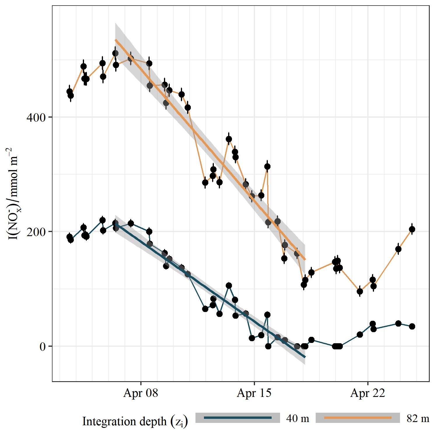
Figure 3Water-column-integrated nitrate inventory. Points show inventory values with error bars indicating standard uncertainty. Lines indicate a linear model fit, with the shaded grey area signifying a 95 % confidence interval.
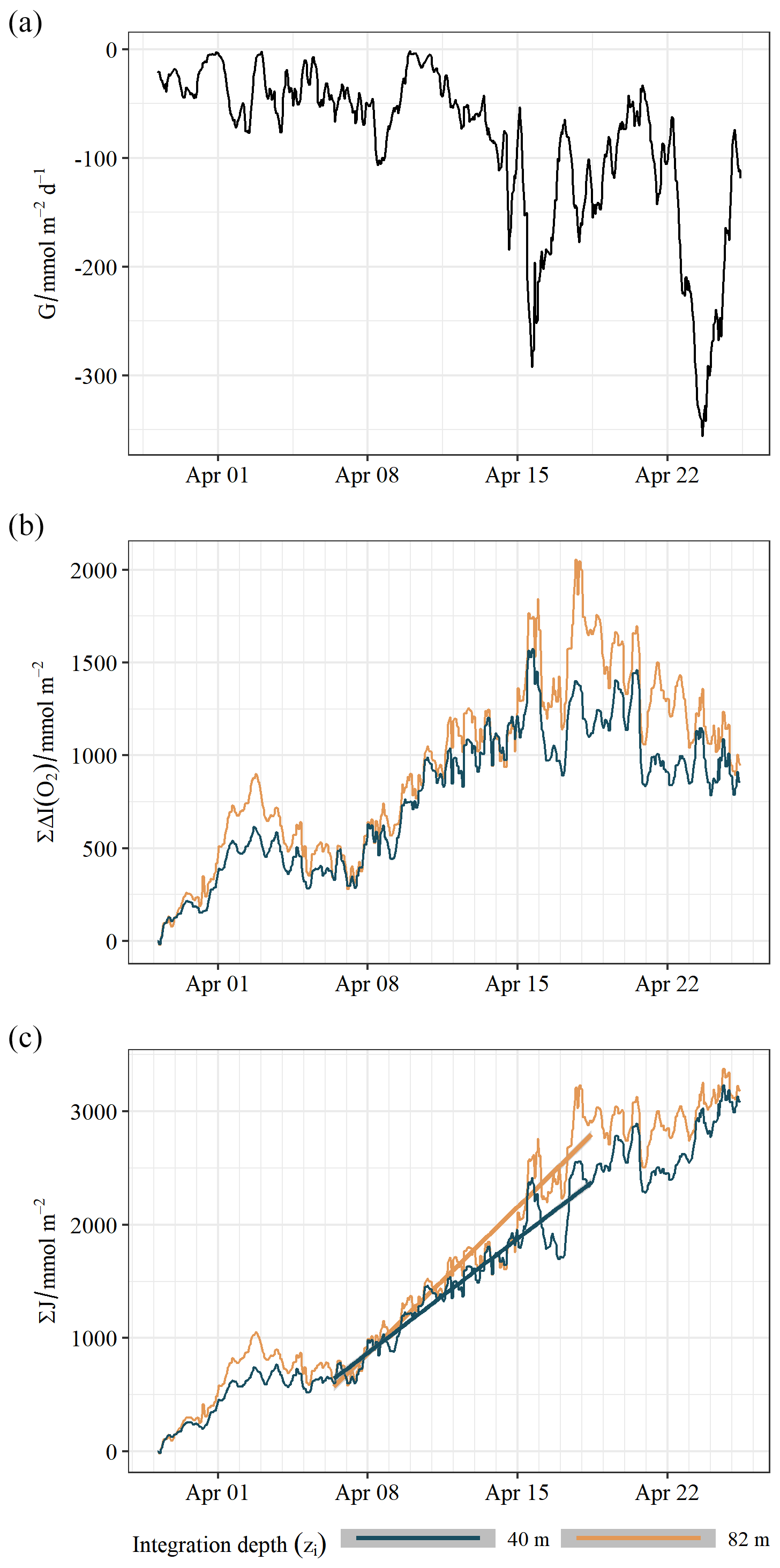
Figure 4Oxygen mass balance. (a) Air–sea oxygen gas exchange with a negative sign signifying a flux out of the ocean. (b) The change in depth-integrated oxygen inventory. (c) Cumulative net community production. Lines indicate linear model fit to the period associated with nitrate drawdown.
3.3 Oxygen-based net community production (J(O2))
At the start of the time series the water column was slightly supersaturated with oxygen (103 %–104 % in the SML and 102 % in the BML). The moderate winds associated with this period (8 to 9 m s−1) would be expected to induce no more than 1 % supersaturation (Liang et al., 2013), which suggests a system which is already productive. There was some degree of supersaturation throughout the mission in both the SML and BML, with maximum supersaturation exceeding 120 % between 19 and 20 April 2019. The water column oxygen inventory changes are shown in Fig. 4b. There is net outgassing of oxygen throughout the mission (Fig. 4a), with cumulatively 2.3 ± 0.1 mol m−2 released to the atmosphere over 27 d. This outgassing is primarily driven by supersaturation through biological production rather than due to warming of the surface waters. Solubility changes account for only 1 % of the observed air–sea oxygen flux during this period. The water column was net productive throughout the mission (Fig. 4c). J(O2) is seen to be increasing until surface is depleted (19 April 2019), when a marked drop in production followed. As such J(O2) follows a pattern consistent with the initiation of the spring bloom followed by limitation. The water column was likely still slightly net autotrophic at the end of April (Fig. 4c). We estimate cumulative net community oxygen production over the observation period of 3.3 ± 0.1 mol m−2 (Fig. 4). As with the mass balance, we compare both the upper 40 m and the full water column with the results tabulated in Table 1.
3.4 O2 : N ratio
Comparing J(O2) and over the bloom observation period we determine the O2:N ratios, which are summarised in Table 2. We note that the uncertainty associated with these ratios is small compared to previous studies using simultaneous fluxes owing to a more tightly constrained oxygen air–sea gas exchange flux (Alkire et al., 2012). The O2:N ratio (Table 2) is substantially higher in the surface mixed layer relative to the rest of the water column. This is in keeping with observations from the Alkire et al. (2012) 3 d North Atlantic spring bloom study, which found a SML O2:N ratio of 14 ± 4.8 and a photic zone (0 to 53 m) ratio of 10 ± 6 for the main bloom period.
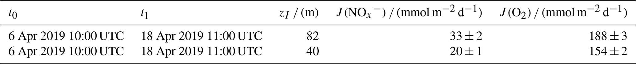
Table 1Summary of inventory changes. Inventories are calculated using either a depth consistent with the mean euphotic depth (zI=40 m) or the full water column (zI=82 m). is net community production in equivalents. J(O2) is net community production in O2 equivalents.
4.1 Metabolic state
Our observations demonstrate a spring bloom which is highly productive and short in duration. A short duration makes it challenging to observe with remote sensing as much of the production is missed entirely due to cloud cover of the study region, typical of coastal seas at temperate latitudes. The water column is already net productive by the time the glider is occupying the transect, with weak stratification seen and partitioning of the oxygen and across the thermocline. While the rates of change in the concentration, relative to the speed of the glider, make the determination of horizontal gradients difficult, we can determine that in the BML concentrations are lower towards the eastern end as seen in Fig. 2. Comparing those concentrations observed near 2∘ E demonstrates a decline in BML concentrations from 4 to 3 mmol m−3. The deepening of the thermocline seen between 11 and 16 April 2019 coincides with the glider moving west, and the subsequent shoaling coincides with the glider moving east. This makes it difficult to determine if this deepening is localised to the western end of the transect. However, differences in wind stress and solar heating are negligible across the transect such that we believe the deepening occurred elsewhere along the transect simultaneously. We therefore suggest that while continues to be consumed, the decline seen in BML concentrations is primarily through dilution and expansion of the BML to incorporate the nutrient-depleted waters from above.
4.2 Stoichiometry of new production
The Redfield ratio considers the remineralisation of an average marine plankton to have a 138:16 (8.6) O2:N ratio. These ratios are known to vary systematically across the global oceans (Li and Peng, 2002). This “traditional” ratio appears applicable to the North Atlantic, with remineralisation ratios for the deep North Atlantic yielding 8.6 ± 1 (Li and Peng, 2002).
The ratios we determine for the central North Sea bloom are lower than those observed in the North Atlantic spring bloom (Table 2). consumption appears to exceed the nitrogen requirements of the average phytoplankton given the observed oxygen production and therefore carbon fixation. However, Redfield ratios are generally not applicable for the whole water column as the simultaneous production of organic matter together with consumption processes modifies the apparent O2:N ratio. This is demonstrated in Fig. 5, where we can see that our observed O2:N ratios could be explained by any number of simultaneous remineralisation processes. Hickman et al. (2012) found wide variations in the uptake ratio associated with changes in the local light climate during summer production in the Celtic Sea. Despite these variations, the particulate organic C:N ratio was observed to be close to the canonical Redfield ratio.
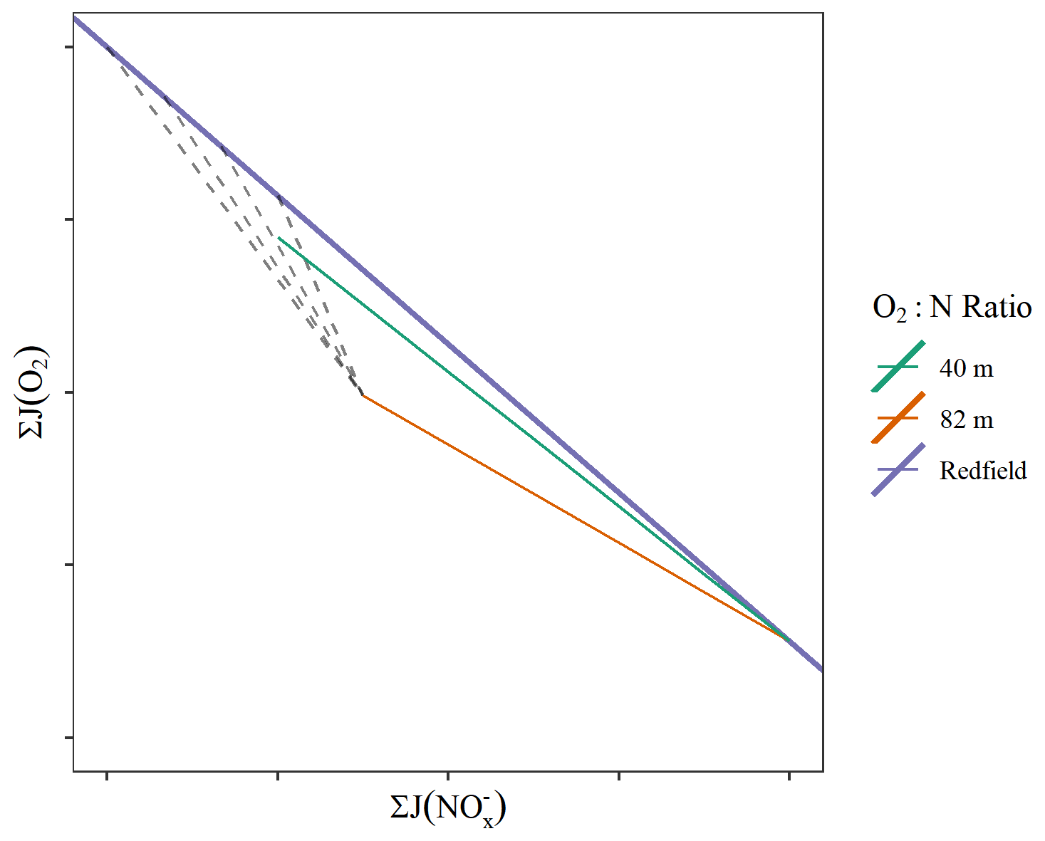
Figure 5Conceptual diagram which shows how the observed O2:N ratios (shown with coloured lines) can be explained by the presence of any number of simultaneous remineralisation processes (dashed lines).

4.3 Comparison with prior regional estimates
Our mean volumetric drawdown rates are also summarised in Table 2 and are comparable to similar prior studies. A previous deployment of the sensor integrated with a Seaglider by Vincent et al. (2018) showed a decline in the surface mixed layer (top 40 m) of −4.3 mmol m−3 over 21 d (4 April to 4–25 April 2015; see Table 2) in the central Celtic Sea during the spring bloom. The 2019 central North Sea spring bloom therefore gave 25 %–150 % faster drawdown rates than the 2015 central Celtic Sea bloom. Direct comparisons of the total inventory change are not possible as the Celtic Sea Seaglider did not sample the stratifying surface waters for during the onset of the 2015 bloom.
The spring bloom in the seasonally stratified regions of the North Sea is thought to represent 40 % of the typical regional annual production (Richardson and Pedersen, 1998). Several previous studies have derived local production estimates for the region north of the Dogger Bank, but these have focused on the summer months (Weston et al., 2005; Bozec et al., 2005). There are relatively few contemporary NCP observations for this region, and most previous studies aggregate their production estimates over very large spatial or temporal scales. Such a broad approach provides limited information to describe production at the spatial and temporal scales comparable to modern biogeochemical models, which operate on <10 km resolution. Where disparities arise between model and observation, it is difficult to determine which regions or processes are inadequately captured. Therefore, accurate advice from the ocean observing community on how models might be improved is heavily constrained.
Richardson and Pedersen (1998) determined the winter nitrate maximum in the central stratified North Sea to be 8 mmol m−3 based on 1993 Convention for the Protection of the Marine Environment of the North-East Atlantic (OSPAR) data, and the 2017 Interim OSPAR Report determined it to be 6 to 8 mmol m−3 between 2006 and 2014. The deployment of a similar glider also fitted with an analyser between November 2017 and January 2018 observed a maximum of 7 ± 0.2 mmol m−3 (Birchill et al., 2021). Using 8 mmol m−3 as the winter nutrient concentration, taking the typical thermocline depth in a given year to be 30 m with zero vertical mixing, and with a C:N ratio of 5.68, they calculated total annual new production for the stratified North Sea to be 1360 ± 680 mmol m−2 (C). By contrast our inventories, with a lower winter nitrate maximum, indicate a total spring bloom new production of 1043 ± 122 mmol m−2 (C) using the above C:N ratio.
Bozec et al. (2006) calculated dissolved-organic-carbon-based NCP for the International Council for the Exploration of the Sea (ICES) regions, which contain the AlterEco transect (no. 4 and no. 14). For comparison we convert these values of NCP to oxygen equivalents using an O2:C ratio of 1.4. This conversion provides a surface mixed layer NCP of 0.93 mmol m−3 d−1 and a bottom water average NCP of −0.14 mmol m−3 d−1 for April (Bozec et al., 2006, do not provide uncertainties). The large temporal and spatial integration range likely fails to resolve much of the local short-term production.
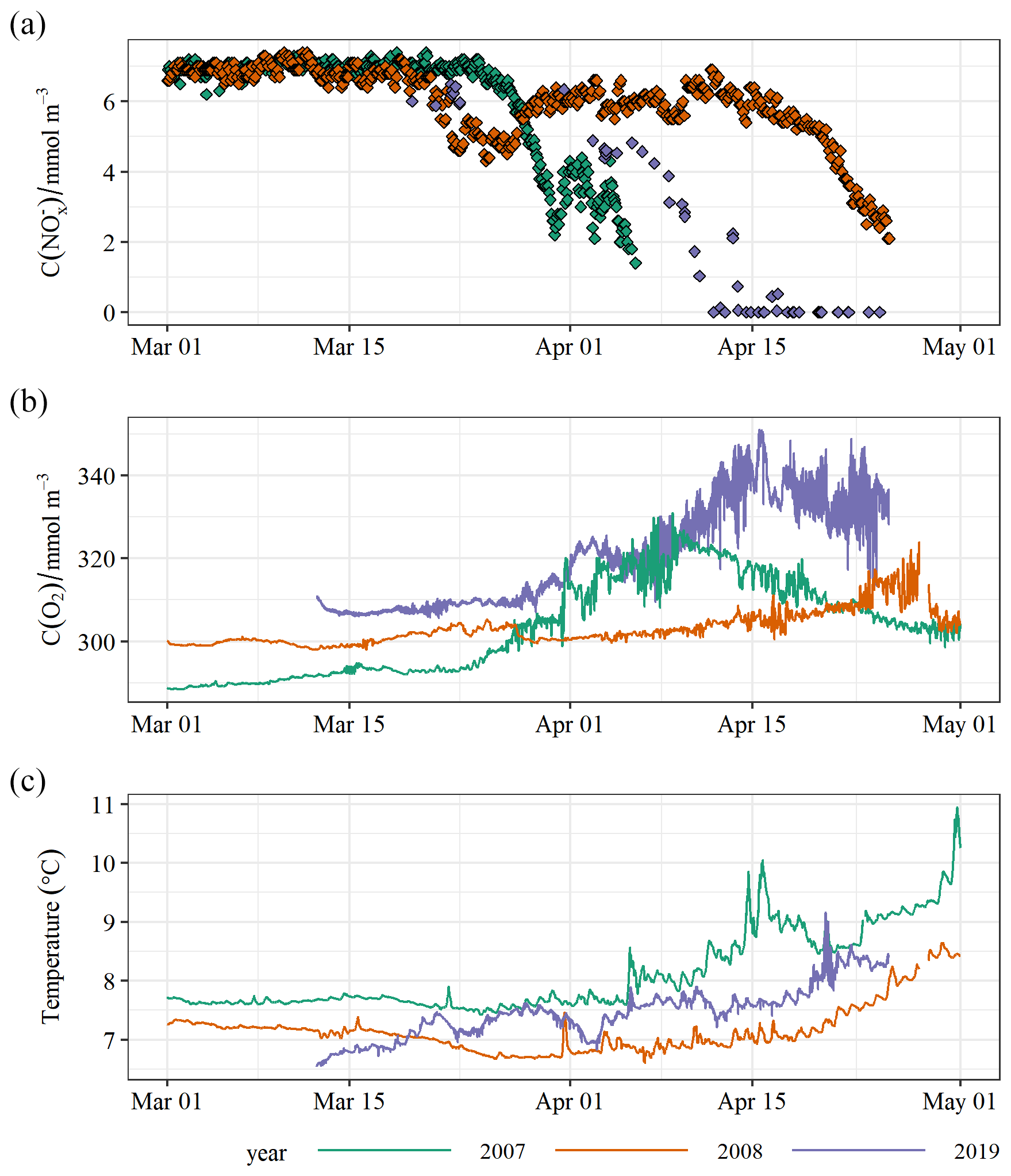
Figure 6 and oxygen concentration observations from the 2007–2008 North Dogger Cefas SmartBuoy mooring together with the 2019 AlterEco Seaglider (this study). and temperature observations are from 1 m depth, while oxygen concentrations are from 25 m in 2007 and 35 m in 2018. For 2019 all data between these depths are shown.
4.4 Interannual variability
Winter concentrations are predicted to reduce in the North Sea due to reduced exchange with the Atlantic Ocean (Gröger et al., 2013). Near-surface and mid-water oxygen from the 2007–2008 Cefas SmartBuoy mooring (Fig. 1) are shown in Fig. 6 together with the comparable Seaglider observations from 2019. We see that the peak concentrations prior to bloom onset are consistently 7 ± 0.5 mmol m−3 across all observed years within this region. The North Sea biogeochemical climatology (Hinrichs et al., 2017) has a single point for comparison: a discrete near-surface sample from February 2000 (7.9 mmol m−3). We therefore do not see any strong evidence for a reduction in peak winter with these data.
Extrapolating observations at the surface buoy to an unknown mixed depth to determine an inventory introduces substantial uncertainties. A more complete knowledge of the water column vertical structure is required to accurately determine NCP rates from these observations. We can use a subset of glider observations to demonstrate this; using only the near-surface value to calculate a 40 m inventory results in a 23 % larger calculated drawdown. However, the trend in Fig. 6 suggests similar maximal rates of consumption.
The duration and intensity of the drawdown demonstrate marked interannual variability. While there is an expected inverse correlation between pre-bloom temperature and oxygen concentration, oxygen saturation does not appear to be solely controlled by differing sea temperatures or bubble injection as 2007 is under-saturated in mid-March (93 %), 2008 is very close to saturation (99 %), and 2019 is 2 %–3 % supersaturated. We note that while there is a general trend of increasing sea surface temperatures in the North Sea (Capuzzo et al., 2018), 2019 was cooler than 2007. Große et al. (2016) suggested that year-to-year variations in the oxygen concentrations are mostly caused by variations in local primary production. Warmer years are thought to induce an earlier spring bloom (Capuzzo et al., 2018). This is reflected in these data, with late-March near-surface sea temperatures coinciding with the observed onset of the bloom.
We present well-resolved production estimates using two complementary methods from the central North Sea using a single autonomous vehicle. These results represent the most complete examination of the spring bloom formation within this region and demonstrate its highly episodic nature, a feature which is typically hard to observe with typical ship surveys or remote sensing. These observations highlight the strength of autonomous vehicles as a key part of future monitoring strategies, complementing remote sensing and biogeochemical modelling efforts. By comparing the rates of NCP through the two methods we determine the O2:N ratio of new production within the water column, finding O2:N ratios in the near surface close to the canonical Redfield North Atlantic ratio, while remineralisation processes in the deeper parts of the water column tend to lower the apparent ratio.
A1 Oxygen NCP model
We can describe the evolution of oxygen over time as the sum of various fluxes:
where CI is the average oxygen concentration within integration depth zI, G is the air–sea gas exchange with a flux into the ocean being defined as positive, M is mixing comprising horizontal (MA) and vertical (Mz) mixing, E is entrainment, A is horizontal advection, and J is net community production.
Air–sea gas exchange is calculated as
where kw is the air–sea transfer velocity parameterisation of Nightingale et al. (2000) derived using the airsea R library (Hull and Johnson, 2015), using the Schmidt number parameterisation of Johnson (2010).
Cs is the near-surface oxygen concentration.
Csat is the concentration of oxygen if it were in equilibrium with the atmosphere at a pressure of 1013.25 hPa (Garcia and Gordon, 1992; using the fit to the Benson and Krause data).
P is local air pressure and P0 standard atmospheric pressure (1013.25 hPa).
B is the wind speed and temperature-dependent bubble supersaturation term from Liang et al. (2013).
This bubble term has a relatively large effect on net community production estimates when Cs is close to Csat (Emerson and Bushinsky, 2016; Hull et al., 2016; Liang et al., 2017).
Gas exchange is only relevant within the ventilated partition of the water column,
which is equivalent to the actively mixed surface layer (known as mixing layer; Brainerd and Gregg, 1995) (zmix). If zI<zmix, then G needs to be scaled by the factor .
Horizontal advection can be described by Eq. (A3).
where is the zonal oxygen gradient, and u is the zonal velocity, with equivalent terms for the meridional (v) direction.

We cannot determine A from our glider data as gliders are semi-Lagrangian; they are displaced by tidal currents, and as such the method of Hull et al. (2020) is not applicable. Gliders are also relativity slow compared with the observed rates of oxygen concentration change and the residual currents along the transect.
We treat the water column as a three-layer system, with an SML and BML separated by a transitional thermocline. Both the SML and BML are considered to be homogeneous, maintained by wind and tidal mixing, respectively. The extent of these layers is typically calculated from the vertical profile of temperature (or density), using the depth at which the temperature is sufficiently different from a reference depth (within the homogeneous layer) as the base of the layer. A reference depth of 10 m, which is commonly used for determining the surface mixed layer depth (zmix) in open-ocean mass balance studies (de Boyer Montégut, 2004; Kara et al., 2000), is inappropriately deep for our data (Fig. 2b). Data within the top 3 m are of poor quality due to the Seaglider surface manoeuvres and wave action. A reference depth of 5 m is therefore chosen as deep enough to avoid biases from poor surface data quality while shallow enough to determine the air–sea oxygen gradient (see Sect. A1). We adopt a temperature-based threshold for zmix of 0.2 ∘C (as per Castro-Morales and Kaiser, 2012), which visually agrees with oxygen profiles (Figs. 2b–d and A1); zmix is therefore defined here as the shallowest depth at which the temperature differs (warmer) from that at 5 m by more than 0.2 ∘C. We reverse the procedure for the bottom mixed layer depth and use the deepest temperature recorded as the reference threshold. The choice of SML or BML definition has minimal impact on our analysis as we do not use the SML as our integration depth for the and O2 mass balance.
Depending on the choice of integration depth, i.e. the volume of water we calculate NCP over, the fluxes to consider change. For example Barone et al. (2019) eliminated the influence of entrainment by defining their integration depth corresponding to an isopycnal, which is always deeper than the base of the surface mixed layer. Often the integration is restricted to the productive part of the water column (euphotic depth; e.g. Bushinsky and Emerson, 2015, or Binetti et al., 2020). However, the shallow nature of the study area presents an opportunity to reduce the overall uncertainty by calculating the change in oxygen inventory over the whole water column, the depth of which is known with a high level of certainty. There is little variation in depth across the E–W transect, and as such we calculate our full water column mass balance in terms of the average total water column depth (zI= (82 ± 0.5) m).
As diurnal warming can reduce the ventilated water column to a region of water above the persistent seasonal thermocline, zmix is not necessarily equivalent to the thermocline depth. It is this volume which is influenced by air–sea gas exchange directly. Typically the dynamic nature of this layer and the difficulty determining its extent from density profiles can introduce significant uncertainties to the magnitude of the air–sea gas flux. The 0.2 ∘C threshold we use to determine the SML visually agrees well with the oxygen profiles used for determining the value of Cs.
By integrating either the entire water column or to a depth which encompasses the BML, our mass balance differential equation is reduced to Eq. (A4): we simply need to estimate the oxygen concentration within the mixing layer for use in determining the gas exchange flux. This also means entrainment and diapycnal mixing fluxes can be ignored as these do not influence the full water column inventory. Rovelli et al. (2016) observed that within the central North Sea these vertical fluxes can be substantial while being both difficult to quantify and temporally variable. Formulating the mass balance to avoid the need for these terms is thus highly advantageous.
In order to best include our systematic and measurement uncertainties we adopt a Bayesian Markov chain Monte Carlo approach to infer our parameter estimates. We implement the probabilistic model described in Eq. (A5), where the operator signifies our observations of the unknown (latent) state parameter. Cs is the concentration of oxygen in the surface actively mixed layer (z<zmix). I is the oxygen concentration integrated over our integration depth (zI); εCs is the uncertainty bias in the oxygen measurements, for this study considered to be ± 1 mmol m−3. This model equates to a 15 % error in kw and a 50 % error in B; εI is calculated as the standard error in I; α, β, and σ are left as improper priors, as in a standard least squares regression. Implementation of this model uses the probabilistic programming language Stan (Carpenter et al., 2017). Output variables are presented with 95 % credible intervals, which are the intervals within which an unobserved parameter value falls with a particular probability. These are therefore analogous to frequentist confidence intervals.
A2 SmartBuoy mooring
The SmartBuoy monitoring station known as “North Dogger” was occupied between 25 February 2007 and 14 September 2008. The moorings consisted of a Cefas ESM2 data logger with an Aanderaa 3835 oxygen optode, Aanderaa 3319B (conductivity and temperature), and an Envirotech NAS-3X nutrient analyser. The NAS-3X performs the same wet-chemistry method as the LoC.
R and STAN code used for this analysis is available by request.
The Seaglider data are available at the British Oceanographic Data Centre (BODC) (https://www.bodc.ac.uk/, British Oceanographic Data Centre, 2021). See also Birchill et al. (2021) for a more thorough description. SmartBuoy data are available at the Cefas Data Portal (https://data.cefas.co.uk/, Cefas Data Portal, 2021).
TH performed the NCP analysis and prepared the original draft. TH, JK, AnB, and NG provided the data curation and validation. TH, AnB, AlB, and MP conducted the glider fieldwork. All authors contributed to experimental design and writing of the manuscript
Alexander Beaton is now a co-founder and employee of Clearwater instruments, which now commercially sells the instrument used in this study. However the instrument for this study was provided by the National Oceanographic Centre (NOC) sensor R&D group.
Publisher’s note: Copernicus Publications remains neutral with regard to jurisdictional claims in published maps and institutional affiliations.
The glider work was funded by the UK National Environment Research Council (NERC; grant numbers NE/P013899/1, NE/P013902/2, NE/P013740/1, NE/P013864/1); the UK government’s Department for Environment, Food and Rural Affairs (Defra); and the World Wide Fund for Nature (WWF). The North Dogger SmartBuoy was funded by Defra (grant nos. ME3205 and SLA25).
This paper was edited by Tina Treude and reviewed by two anonymous referees.
Alkire, M. B., D'Asaro, E., Lee, C., Jane Perry, M., Gray, A., Cetinić, I., Briggs, N., Rehm, E., Kallin, E., Kaiser, J., and González-Posada, A.: Estimates of Net Community Production and Export Using High-Resolution, Lagrangian Measurements of O2, NO3−, and POC through the Evolution of a Spring Diatom Bloom in the North Atlantic, Deep-Sea Res. Pt. I, 64, 157–174, 2012. a, b, c, d, e
Alkire, M. B., Lee, C. M., a. D'Asaro, E., Perry, M. J., Briggs, N. T., Cetinić, I., and Gray, A. M.: Net Community Production and Export from Seaglider Measurements in the North Atlantic after the Spring Bloom, J. Geophys. Res.-Ocean., 119, 6121–6139, https://doi.org/10.1002/2014jc010105, 2014. a
Anderson, L. A. and Sarmiento, J. L.: Redfield Ratios of Remineralization Determined by Nutrient Data Analysis, Global Biogeochem. Cy., 8, 65–80, https://doi.org/10.1029/93gb03318, 1994. a
Barone, B., Nicholson, D., Ferrón, S., Firing, E., and Karl, D.: The Estimation of Gross Oxygen Production and Community Respiration from Autonomous Time-series Measurements in the Oligotrophic Ocean, Limnol. Oceanogr.-Method., 17, lom3.10340, https://doi.org/10.1002/lom3.10340, 2019. a
Bauer, J. E., Cai, W.-J., Raymond, P. A., Bianchi, T. S., Hopkinson, C. S., and Regnier, P. A. G.: The Changing Carbon Cycle of the Coastal Ocean, Nature, 504, 61–70, https://doi.org/10.1038/nature12857, 2013. a, b
Beaton, A. D., Cardwell, C. L., Thomas, R. S., Sieben, V. J., Legiret, F.-E., Waugh, E. M., Statham, P. J., Mowlem, M. C., and Morgan, H.: Lab-on-Chip Measurement of Nitrate and Nitrite for In Situ Analysis of Natural Waters, Environ. Sci. Technol., 46, 9548–9556, https://doi.org/10.1021/es300419u, 2012. a, b, c
Binetti, U., Kaiser, J., Damerell, G. M., Rumyantseva, A., Martin, A. P., Henson, S., and Heywood, K. J.: Net Community Oxygen Production Derived from Seaglider Deployments at the Porcupine Abyssal Plain Site (PAP; Northeast Atlantic) in 2012–13, Prog. Oceanogr., 183, 102293, https://doi.org/10.1016/j.pocean.2020.102293, 2020. a
Birchill, A., Beaton, A. D., Pascal, R. W., Hull, T., and Kaiser, J.: An Alternative Framework to Assess Marine Ecosystem Functioning in Shelf Seas (AlterEco) Post-Recovery Seaglider Lab-on-a-Chip (LoC) Nitrate + Nitrite (NOx) Data between November 2017 and April 2019 in the North Sea, BODC [data set], https://doi.org/10/f984, 2021. a, b
Bittig, H. C., Körtzinger, A., Neill, C., van Ooijen, E., Plant, J. N., Hahn, J., Johnson, K. S., Yang, B., and Emerson, S. R.: Oxygen Optode Sensors: Principle, Characterization, Calibration, and Application in the Ocean, Front. Mar. Sci., 4, 1–25, https://doi.org/10.3389/fmars.2017.00429, 2018. a, b, c
Bozec, Y., Thomas, H., Elkalay, K., and De Baar, H. J.: The Continental Shelf Pump for CO2 in the North Sea – Evidence from Summer Observation, Mar. Chem., 93, 131–147, https://doi.org/10.1016/j.marchem.2004.07.006, 2005. a
Bozec, Y., Thomas, H., Schiettecatte, L.-S., Borges, A. V., Elkalay, K., and de Baar, H. J. W.: Assessment of the Processes Controlling the Seasonal Variations of Dissolved Inorganic Carbon in the North Sea, Limnol. Oceanogr., 51, 2746–2762, https://doi.org/10.4319/lo.2006.51.6.2746, 2006. a, b, c
Brainerd, K. E. and Gregg, M. C.: Surface Mixed and Mixing Layer Depths, Deep-Sea Res. Pt. I, 42, 1521–1543, https://doi.org/10.1016/0967-0637(95)00068-h, 1995. a
British Oceanographic Data Centre (BODC): https://www.bodc.ac.uk/, last access: 15 September 2021.
Burson, A., Stomp, M., Akil, L., Brussaard, C. P. D., and Huisman, J.: Unbalanced Reduction of Nutrient Loads Has Created an Offshore Gradient from Phosphorus to Nitrogen Limitation in the North Sea, Limnol. Oceanogr., 61, 869–888, https://doi.org/10.1002/lno.10257, 2016. a
Bushinsky, S. M. and Emerson, S.: Marine Biological Production from in Situ Oxygen Measurements on a Profiling Float in the Subarctic Pacific Ocean, Global Biogeochem. Cy., 29, 2050–2060, https://doi.org/10.1002/2015gb005251, 2015. a
Capuzzo, E., Lynam, C. P., Barry, J., Stephens, D., Forster, R. M., Greenwood, N., McQuatters-Gollop, A., Silva, T., van Leeuwen, S. M., and Engelhard, G. H.: A Decline in Primary Production in the North Sea over 25 Years, Associated with Reductions in Zooplankton Abundance and Fish Stock Recruitment, Glob. Change Biol., 24, e352–e364, https://doi.org/10.1111/gcb.13916, 2018. a, b
Carpenter, B., Gelman, A., Hoffman, M. D., Lee, D., Goodrich, B., Betancourt, M., Brubaker, M., Guo, J., Li, P., and Riddell, A.: Stan : A Probabilistic Programming Language, 76, 1–32, https://doi.org/10.18637/jss.v076.i01, 2017. a
Castro-Morales, K. and Kaiser, J.: Using Dissolved Oxygen Concentrations to Determine Mixed Layer Depths in the Bellingshausen Sea, Ocean Sci., 8, 1–10, https://doi.org/10.5194/os-8-1-2012, 2012. a
Cefas Data Portal: https://data.cefas.co.uk/, last access: 15 September 2021.
Copernicus, C. C. S.: ERA5: Fifth Generation of ECMWF Atmospheric Reanalyses of the Global Climate, CDS [data set], https://doi.org/10.24381/cds.bd0915c6, 2018. a
de Boyer Montégut, C.: Mixed Layer Depth over the Global Ocean: An Examination of Profile Data and a Profile-Based Climatology, J. Geophys. Res., 109, C12003, https://doi.org/10.1029/2004jc002378, 2004. a
Emeis, K.-C., van Beusekom, J., Callies, U., Ebinghaus, R., Kannen, A., Kraus, G., Kröncke, I., Lenhart, H., Lorkowski, I., Matthias, V., Möllmann, C., Pätsch, J., Scharfe, M., Thomas, H., Weisse, R., and Zorita, E.: The North Sea – A Shelf Sea in the Anthropocene, J. Mar. Syst., 141, 18–33, https://doi.org/10.1016/j.jmarsys.2014.03.012, 2015. a, b, c, d, e
Emerson, S. and Bushinsky, S.: The Role of Bubbles during Air-Sea Gas Exchange, J. Geophys. Res.-Ocean., 121, 4360–4376, https://doi.org/10.1002/2016jc011744, 2016. a
Garau, B., Ruiz, S., Zhang, W. G., Pascual, A., Heslop, E., Kerfoot, J., and Tintoré, J.: Thermal Lag Correction on Slocum CTD Glider Data, J. Atmos. Ocean. Technol., 28, 1065–1071, https://doi.org/10.1175/jtech-d-10-05030.1, 2011. a
Garcia, H. E. and Gordon, L. I.: Oxygen Solubility in Seawater: Better Fitting Equations, Limnol. Oceanogr., 37, 1307–1312, https://doi.org/10.4319/lo.1992.37.6.1307, 1992. a
GEBCO, B. C. G.: The GEBCO_2019 Grid – a Continuous Terrain Model of the Global Oceans and Land, BODC [data set], https://doi.org/10.5285/836F016A-33BE-6DDC-E053-6C86ABC0788E, 2019. a, b, c
Graham, J. A., O'Dea, E., Holt, J., Polton, J., Hewitt, H. T., Furner, R., Guihou, K., Brereton, A., Arnold, A., Wakelin, S., Castillo Sanchez, J. M., and Mayorga Adame, C. G.: AMM15: A New High-Resolution NEMO Configuration for Operational Simulation of the European North-West Shelf, Geosci. Model Dev., 11, 681–696, https://doi.org/10.5194/gmd-11-681-2018, 2018. a
Greenwood, N.: SmartBuoy Observational Network – North Dogger, Cefas [data set], https://doi.org/10.14466/CEFASDATAHUB.29, 2016. a
Greenwood, N., Parker, E. R., Fernand, L., Sivyer, D. B., Weston, K., Painting, S. J., Kröger, S., Forster, R. M., Lees, H. E., Mills, D. K., and Laane, R. W. P. M.: Detection of Low Bottom Water Oxygen Concentrations in the North Sea; Implications for Monitoring and Assessment of Ecosystem Health, Biogeosciences, 7, 1357–1373, https://doi.org/10.5194/bg-7-1357-2010, 2010. a
Gröger, M., Maier-Reimer, E., Mikolajewicz, U., Moll, A., and Sein, D.: NW European Shelf under Climate Warming: Implications for Open Ocean – Shelf Exchange, Primary Production, and Carbon Absorption, Biogeosciences, 10, 3767–3792, https://doi.org/10.5194/bg-10-3767-2013, 2013. a
Große, F., Greenwood, N., Kreus, M., Lenhart, H.-J., Machoczek, D., Pätsch, J., Salt, L., and Thomas, H.: Looking beyond Stratification: A Model-Based Analysis of the Biological Drivers of Oxygen Deficiency in the North Sea, Biogeosciences, 13, 2511–2535, https://doi.org/10.5194/bg-13-2511-2016, 2016. a, b, c
Halpern, B. S., Longo, C., Lowndes, J. S. S., Best, B. D., Frazier, M., Katona, S. K., Kleisner, K. M., Rosenberg, A. A., Scarborough, C., and Selig, E. R.: Patterns and Emerging Trends in Global Ocean Health, PLOS ONE, 10, e0117863, https://doi.org/10.1371/journal.pone.0117863, 2015. a
Harris, P. T., Macmillan-Lawler, M., Rupp, J., and Baker, E. K.: Geomorphology of the Oceans, Mar. Geol., 352, 4–24, https://doi.org/10.1016/j.margeo.2014.01.011, 2014. a
Hickman, A., Moore, C., Sharples, J., Lucas, M., Tilstone, G., Krivtsov, V., and Holligan, P.: Primary Production and Nitrate Uptake within the Seasonal Thermocline of a Stratified Shelf Sea, Mar. Ecol. Prog. Ser., 463, 39–57, https://doi.org/10.3354/meps09836, 2012. a
Hill, A. E., Brown, J., Fernand, L., Holt, J., Horsburgh, K. J., Proctor, R., Raine, R., and Turrell, W. R.: Thermohaline Circulation of Shallow Tidal Seas, Geophys. Res. Lett., 35, L11605, https://doi.org/10.1029/2008gl033459, 2008. a
Hinrichs, I., Gouretski, V., Pätsch, J., Emeis, K.-C., and Stammer, D.: North Sea Biogeochemical Climatology (Version 1.1), https://doi.org/10.1594/WDCC/NSBCLIM_V1.1, 2017. a
Hull, T. and Johnson, M.: Airsea: R Tools for Air-Sea Gas Exchange Studies (0.2), Cefas, https://doi.org/10.5281/zenodo.45656, 2015. a
Hull, T. and Kaiser, J.: AlterEco Post-Recovery Seaglider Data between November 2017 and April 2019 in the North Sea, BODC [data set], https://doi.org/10/fk8m, 2020. a
Hull, T., Greenwood, N., Kaiser, J., and Johnson, M.: Uncertainty and Sensitivity in Optode-Based Shelf-Sea Net Community Production Estimates, Biogeosciences, 13, 943–959, https://doi.org/10.5194/bg-13-943-2016, 2016. a, b, c, d
Hull, T., Johnson, M., Greenwood, N., and Kaiser, J.: Bottom Mixed Layer Oxygen Dynamics in the Celtic Sea, Biogeochemistry, 149, 263–289, 2020. a
Johnson, K. S., Coletti, L. J., and Chavez, F. P.: Diel Nitrate Cycles Observed with in Situ Sensors Predict Monthly and Annual New Production, Deep-Sea Res. Pt. I, 53, 561–573, https://doi.org/10.1016/j.dsr.2005.12.004, 2006. a
Johnson, M. T.: A Numerical Scheme to Calculate Temperature and Salinity Dependent Air-Water Transfer Velocities for Any Gas, Ocean Sci., 6, 913–932, https://doi.org/10.5194/os-6-913-2010, 2010. a
Kara, A. B., Rochford, P. A., and Hurlburt, H. E.: An Optimal Definition for Ocean Mixed Layer Depth, J. Geophys. Res.-Ocean., 105, 16803–16821, https://doi.org/10.1029/2000jc900072, 2000. a
Kitidis, V., Shutler, J. D., Ashton, I., Warren, M., Brown, I., Findlay, H., Hartman, S. E., Sanders, R., Humphreys, M., Kivimäe, C., Greenwood, N., Hull, T., Pearce, D., McGrath, T., Stewart, B. M., Walsham, P., McGovern, E., Bozec, Y., Gac, J.-P., van Heuven, S. M. A. C., Hoppema, M., Schuster, U., Johannessen, T., Omar, A., Lauvset, S. K., Skjelvan, I., Olsen, A., Steinhoff, T., Körtzinger, A., Becker, M., Lefevre, N., Diverrès, D., Gkritzalis, T., Cattrijsse, A., Petersen, W., Voynova, Y. G., Chapron, B., Grouazel, A., Land, P. E., Sharples, J., and Nightingale, P. D.: Winter Weather Controls Net Influx of Atmospheric CO2 on the North-West European Shelf, Sci. Rep., 9, 20153, https://doi.org/10/gg5sc5, 2019. a
Legge, O., Johnson, M., Hicks, N., Jickells, T., Diesing, M., Aldridge, J., Andrews, J., Artioli, Y., Bakker, D. C. E., Burrows, M. T., Carr, N., Cripps, G., Felgate, S. L., Fernand, L., Greenwood, N., Hartman, S., Kröger, S., Lessin, G., Mahaffey, C., Mayor, D. J., Parker, R., Queirós, A. M., Shutler, J. D., Silva, T., Stahl, H., Tinker, J., Underwood, G. J. C., Van Der Molen, J., Wakelin, S., Weston, K., and Williamson, P.: Carbon on the Northwest European Shelf: Contemporary Budget and Future Influences, Front. Mar. Sci., 7, 143, https://doi.org/10.3389/fmars.2020.00143, 2020. a
Li, Y.-H. and Peng, T.-H.: Latitudinal Change of Remineralization Ratios in the Oceans and Its Implication for Nutrient Cycles, Global Biogeochem. Cy., 16, 77-1–77-16, https://doi.org/10.1029/2001gb001828, 2002. a, b
Liang, J.-H., Deutsch, C., McWilliams, J. C., Baschek, B., Sullivan, P. P., and Chiba, D.: Parameterizing Bubble-Mediated Air-Sea Gas Exchange and Its Effect on Ocean Ventilation, Global Biogeochem. Cy., 27, 894–905, https://doi.org/10.1002/gbc.20080, 2013. a, b
Liang, J.-H., Emerson, S. R., D'Asaro, E. A., McNeil, C. L., Harcourt, R. R., Sullivan, P. P., Yang, B., and Cronin, M. F.: On the Role of Sea-State in Bubble-Mediated Air-Sea Gas Flux during a Winter Storm, J. Geophys. Res.-Ocean., 122, 2671–2685, https://doi.org/10.1002/2016jc012408, 2017. a
Mathis, M., Elizalde, A., Mikolajewicz, U., and Pohlmann, T.: Variability Patterns of the General Circulation and Sea Water Temperature in the North Sea, Prog. Oceanogr., 135, 91–112, https://doi.org/10.1016/j.pocean.2015.04.009, 2015. a
Nielsen, T., Løkkegaard, B., Richardson, K., Bo Pedersen, R., and Hansen, L.: Structure of Plankton Communities in the Dogger Bank Area (North Sea) during a Stratified Situation, Mar. Ecol. Prog. Ser., 95, 115–131, 1993. a, b
Nightingale, P. D., Malin, G., Law, C. S., Watson, A. J., Liss, P. S., Liddicoat, M. I., Boutin, J., and Upstill-Goddard, R. C.: In Situ Evaluation of Air-Sea Gas Exchange Parameterizations Using Novel Conservative and Volatile Tracers, Global Biogeochem. Cy., 14, 373–387, https://doi.org/10.1029/1999gb900091, 2000. a
Palevsky, H. I., Ribalet, F., Swalwell, J. E., Cosca, C. E., Cokelet, E. D., Feely, R. A., Armbrust, E. V., and Quay, P. D.: The Influence of Net Community Production and Phytoplankton Community Structure on CO2 Uptake in the Gulf of Alaska: Gulf of Alaska NCP, Phytoplankton, and CO2, Global Biogeochem. Cy., 27, 664–676, https://doi.org/10.1002/gbc.20058, 2013. a
Plant, J. N., Johnson, K. S., Sakamoto, C. M., Jannasch, H. W., Coletti, L. J., Riser, S. C., and Swift, D. D.: Net Community Production at Ocean Station Papa Observed with Nitrate and Oxygen Sensors on Profiling Floats, Global Biogeochem. Cy., 30, 859–879, https://doi.org/10.1002/2015gb005349, 2016. a, b
Plumeridge, A. A. and Roberts, C. M.: Conservation Targets in Marine Protected Area Management Suffer from Shifting Baseline Syndrome: A Case Study on the Dogger Bank, Mar. Pollut. Bull., 116, 395–404, 2017. a
Queste, B.: Hydrographic Observations of Oxygen and Related Physical Variables in the North Sea and Western Ross Sea Polynya, University of East Anglia, UK, 2013. a
Queste, B. Y., Fernand, L., Jickells, T. D., and Heywood, K. J.: Spatial Extent and Historical Context of North Sea Oxygen Depletion in August 2010, Biogeochemistry, 113, 53–68, 2013. a
Richardson, K. and Pedersen, F. B.: Estimation of New Production in the North Sea: Consequences for Temporal and Spatial Variability of Phytoplankton, ICES J. Mar. Sci., 55, 574–580, https://doi.org/10.1006/jmsc.1998.0402, 1998. a, b
Riegman, R., Malschaert, H., and Colijn, F.: Primary Production of Phytoplankton at a Frontal Zone Located at the Northern Slope of the Dogger Bank (North Sea), Mar. Biol., 105, 329–336, https://doi.org/10.1007/bf01344303, 1990. a
Rovelli, L., Dengler, M., Schmidt, M., Sommer, S., Linke, P., and McGinnis, D. F.: Thermocline Mixing and Vertical Oxygen Fluxes in the Stratified Central North Sea, Biogeosciences, 13, 1609–1620, https://doi.org/10.5194/bg-13-1609-2016, 2016. a, b, c
Sharples, J., Mayor, D. J., Poulton, A. J., Rees, A. P., and Robinson, C.: Shelf Sea Biogeochemistry: Nutrient and Carbon Cycling in a Temperate Shelf Sea Water Column, Prog. Oceanogr., 177, 102182, https://doi.org/10.1016/j.pocean.2019.102182, 2019. a
Tengberg, A. and Hovdenes, J.: Information on Long-Term Stability and Accuracy of Aanderaa Oxygen Optodes. Information about Multipoint Calibration System and Sensor Option Overview., Tech. rep., Aanderaa Data Instruments, 2014. a
Thomas, H.: Enhanced Open Ocean Storage of CO2 from Shelf Sea Pumping, Science, 304, 1005–1008, 2004. a
Thomas, H., Bozec, Y., Elkalay, K., de Baar, H. J. W., Borges, A. V., and Schiettecatte, L.-S.: Controls of the Surface Water Partial Pressure of CO2 in the North Sea, Biogeosciences, 2, 323–334, https://doi.org/10.5194/bg-2-323-2005, 2005. a
Uchida, H., Kawano, T., Kaneko, I., and Fukasawa, M.: In Situ Calibration of Optode-Based Oxygen Sensors, J. Atmos. Ocean. Technol., 25, 2271–2281, https://doi.org/10.1175/2008jtecho549.1, 2008. a
Vincent, A. G., Pascal, R. W., Beaton, A. D., Walk, J., Hopkins, J. E., Woodward, E. M. S., Mowlem, M., and Lohan, M. C.: Nitrate Drawdown during a Shelf Sea Spring Bloom Revealed Using a Novel Microfluidic in Situ Chemical Sensor Deployed within an Autonomous Underwater Glider, Mar. Chem., 205, 29–36, https://doi.org/10.1016/j.marchem.2018.07.005, 2018. a, b, c, d, e, f, g, h
Wakelin, S. L., Artioli, Y., Holt, J. T., Butenschön, M., and Blackford, J.: Controls on Near-Bed Oxygen Concentration on the Northwest European Continental Shelf under a Potential Future Climate Scenario, Prog. Oceanogr., 187, 102400, https://doi.org/10.1016/j.pocean.2020.102400, 2020. a
Weston, K., Fernand, L., Mills, D. K., Delahunty, R., and Brown, J.: Primary Production in the Deep Chlorophyll Maximum of the Central North Sea, J. Plankton Res., 27, 909–922, 2005. a, b
Wihsgott, J. U., Sharples, J., Hopkins, J. E., Woodward, E. M. S., Hull, T., Greenwood, N., and Sivyer, D. B.: Observations of Vertical Mixing in Autumn and Its Effect on the Autumn Phytoplankton Bloom, Prog. Oceanogr., 177, 102059, https://doi.org/10.1016/j.pocean.2019.01.001, 2019. a