the Creative Commons Attribution 4.0 License.
the Creative Commons Attribution 4.0 License.
 | 29 Jan 2021
Implementation of nitrogen cycle in the CLASSIC land model
Ali Asaadi
Vivek K. Arora
A terrestrial nitrogen (N) cycle model is coupled to the carbon (C) cycle in the framework of the Canadian Land Surface Scheme Including Biogeochemical Cycles (CLASSIC). CLASSIC currently models physical and biogeochemical processes and simulates fluxes of water, energy, and CO2 at the land–atmosphere boundary. CLASSIC is similar to most models and its gross primary productivity increases in response to increasing atmospheric CO2 concentration. In the current model version, a downregulation parameterization emulates the effect of nutrient constraints and scales down potential photosynthesis rates, using a globally constant scalar, as a function of increasing CO2. In the new model when nitrogen (N) and carbon (C) cycles are coupled, cycling of N through the coupled soil–vegetation system facilitates the simulation of leaf N amount and maximum carboxylation capacity (Vcmax) prognostically. An increase in atmospheric CO2 decreases leaf N amount and therefore Vcmax, allowing the simulation of photosynthesis downregulation as a function of N supply. All primary N cycle processes that represent the coupled soil–vegetation system are modelled explicitly. These include biological N fixation; treatment of externally specified N deposition and fertilization application; uptake of N by plants; transfer of N to litter via litterfall; mineralization; immobilization; nitrification; denitrification; ammonia volatilization; leaching; and the gaseous fluxes of NO, N2O, and N2. The interactions between terrestrial C and N cycles are evaluated by perturbing the coupled soil–vegetation system in CLASSIC with one forcing at a time over the 1850–2017 historical period. These forcings include the increase in atmospheric CO2, change in climate, increase in N deposition, and increasing crop area and fertilizer input, over the historical period. An increase in atmospheric CO2 increases the C:N ratio of vegetation; climate warming over the historical period increases N mineralization and leads to a decrease in the vegetation C:N ratio; N deposition also decreases the vegetation C:N ratio. Finally, fertilizer input increases leaching, NH3 volatilization, and gaseous losses of N2, N2O, and NO. These model responses are consistent with conceptual understanding of the coupled C and N cycles. The simulated terrestrial carbon sink over the 1959–2017 period, from the simulation with all forcings, is 2.0 Pg C yr−1 and compares reasonably well with the quasi observation-based estimate from the 2019 Global Carbon Project (2.1 Pg C yr−1). The contribution of increasing CO2, climate change, and N deposition to carbon uptake by land over the historical period (1850–2017) is calculated to be 84 %, 2 %, and 14 %, respectively.
- Article
(10838 KB) - Full-text XML
- BibTeX
- EndNote


The works published in this journal are distributed under the Creative Commons Attribution 4.0 License. This license does not affect the Crown copyright work, which is re-usable under the Open Government Licence (OGL). The Creative Commons Attribution 4.0 License and the OGL are interoperable and do not conflict with, reduce or limit each other.
© Crown copyright 2021
The uptake of carbon (C) by land and ocean in response to the increase in anthropogenic fossil fuel emissions of CO2 has served to slow down the growth rate of atmospheric CO2 since the start of the industrial revolution. At present, about 55 % of total carbon emitted into the atmosphere is taken up by land and oceans (Le Quéré et al., 2018; Friedlingstein et al., 2019). It is of great policy, societal, and scientific relevance whether land and oceans will continue to provide this ecosystem service. Over land, as long as photosynthesis is not water limited, the uptake of carbon in response to increasing anthropogenic CO2 emissions is driven by two primary factors: (1) the CO2 fertilization of the terrestrial biosphere and (2) the increase in temperature, both of which are associated with increasing [CO2]. The CO2 fertilization effect increases photosynthesis rates for about 80 % of the world's vegetation that uses the C3 photosynthetic pathway and is currently limited by [CO2] (Still et al., 2003; Zhu et al., 2016). The remaining 20 % of vegetation uses the C4 photosynthetic pathway that is much less sensitive to [CO2]. Warming increases carbon uptake by vegetation in mid- to high-latitude regions where growth is currently limited by low temperatures (Zeng et al., 2011).
Even when atmospheric CO2 is not limiting for photosynthesis and near-surface air temperature is optimal, vegetation cannot photosynthesize at its maximum possible rate if available water and nutrients (most importantly nitrogen (N) and phosphorus (P)) constrain photosynthesis (Vitousek and Howarth, 1991; Reich et al., 2006b). In the absence of water and nutrients, photosynthesis simply cannot occur. N is a major component of chlorophyll (the compound through which plants photosynthesize) and amino acids (which are the building blocks of proteins). The constraint imposed by available water and nutrients implies that the carbon uptake by land over the historical period in response to increasing [CO2] is lower than what it would have been if water and nutrients were not limiting. This lower-than-maximum theoretically possible rate of increase in photosynthesis in response to increasing atmospheric CO2 is referred to as downregulation (Faria et al., 1996; Sanz-Sáez et al., 2010). Typically, however, the term downregulation of photosynthesis is used only in the context of nutrients and not in the context of water. Downregulation is defined as a decrease in the photosynthetic capacity of plants grown at elevated CO2 in comparison to plants grown at baseline CO2 (McGuire et al., 1995). However, despite the decrease in photosynthetic capacity, the photosynthesis rate for plants grown at elevated CO2 is still higher than the rate for plants grown and measured at baseline CO2 because of higher background CO2.
Earth system models (ESMs) that explicitly represent coupling of the global carbon cycle and physical climate system processes are the only tools available at present that, in a physically consistent way, are able to project how land and ocean carbon cycles will respond to future changes in [CO2]. Such models are routinely compared to one another under the auspices of the Coupled Model Intercomparison Project (CMIP) every 6–7 years. The most recent and sixth phase of CMIP (CMIP6) is currently underway (Eyring et al., 2016). Interactions between the carbon cycle and climate in ESMs have been compared under the umbrella of the Coupled Climate–Carbon Cycle Model Intercomparison Project (C4MIP) (Jones et al., 2016) which is an approved model intercomparison project (MIP) of the CMIP. Comparison of land and ocean carbon uptake in C4MIP studies (Friedlingstein et al., 2006; Arora et al., 2013, 2020) indicates that the inter-model uncertainty in future land carbon uptake across ESMs is more than 3 times than the uncertainty for the ocean carbon uptake. The reason for widely varying estimates of future land carbon uptake is that our understanding of biological processes that determine land carbon uptake is much less advanced than the physical processes which primarily determine carbon uptake over the ocean. In the current generation of terrestrial ecosystem models, other than leaf-level photosynthesis for which a theoretical framework exists, almost all of the biological processes are represented on the basis of empirical observations and parameterized in one way or another. In addition, not all models include nutrient cycles. In the absence of an explicit representation of nutrient constraints on photosynthesis, land models in ESMs parameterize downregulation of photosynthesis in other ways that reduce the rate of increase in photosynthesis to values below its theoretically maximum possible rate, as [CO2] increases (e.g., Arora et al., 2009). Comparison of models across the fifth and sixth phase of CMIP shows that the fraction of models with a land N cycle is increasing (Arora et al., 2013, 2020).
The nutrient constraints on photosynthesis are well recognized (Vitousek and Howarth, 1991; Arneth et al., 2010). Terrestrial carbon cycle models' neglect of nutrient limitation on photosynthesis has been questioned from an ecological perspective (Reich et al., 2006a), and it has been argued that without nutrient constraints these models will overestimate future land carbon uptake (Hungate et al., 2003). Since in the real world photosynthesis downregulation does indeed occur due to nutrient constraints, it may be argued that more confidence can be placed in future projections of models that explicitly model the interactions between the terrestrial C and N cycles rather than parameterize it in some other way.
Here, we present the implementation of the N cycle in the Canadian Land Surface Scheme Including Biogeochemical Cycles (CLASSIC) model, which serves as the land component in the family of Canadian Earth System models (Arora et al., 2009, 2011; Swart et al., 2019). Section 2 briefly describes existing physical and carbon cycle components and processes of the CLASSIC model. The conceptual basis of the new N cycle model and its parameterizations are described in Sect. 3. Section 4 outlines the methodology and data sets that we have used to perform various simulations over the 1850–2017 historical period to assess the realism of the coupled C and N cycles in CLASSIC in response to various forcings. Results from these simulations over the historical period are presented in Sect. 5, and finally discussion and conclusions are presented in Sect. 6.
2.1 The physical and carbon biogeochemical processes
The CLASSIC model is the successor to, and based on, the coupled Canadian Land Surface Scheme (CLASS; Verseghy, 1991; Verseghy et al., 1993) and Canadian Terrestrial Ecosystem Model (CTEM; Arora and Boer, 2005; Melton and Arora, 2016). CLASS and CTEM model physical and biogeochemical processes in CLASSIC, respectively. Both CLASS and CTEM have a long history of development as described in Melton et al. (2020), who also provide an overview of the CLASSIC land model and describe its new technical developments that launched CLASSIC as a community model. CLASSIC simulates land–atmosphere fluxes of water, energy, momentum, CO2, and CH4. The CLASSIC model can be run at a point scale, e.g., using meteorological and geophysical data from a FLUXNET site, or over a spatial domain, that may be global or regional, using gridded data. We briefly summarize the primary physical and carbon biogeochemical processes of CLASSIC here that are relevant in the context of implementation of the N cycle in the model.
2.1.1 Physical processes
The physical processes of CLASSIC which simulate fluxes of water, energy, and momentum are calculated over vegetated, snow, and bare fractions on a model grid at a sub-daily time step of 30 min. The vegetation is described in terms of four plant functional types (PFTs): needleleaf trees, broadleaf trees, crops, and grasses. In the current study, the fractional coverage of these four PFTs are specified over the historical period. The structural attributes of vegetation are described by the leaf area index (LAI), vegetation height, canopy mass, and rooting distribution through the soil layers, and these are all simulated dynamically by the biogeochemical module of CLASSIC. In the model version used here, 20 ground layers starting with 10 layers of 0.1 m thickness are used. The thickness of layers gradually increases to 30 m for a total ground depth of over 61 m. The depth to bedrock varies geographically and is specified based on a soil depth data set. Liquid and frozen soil moisture contents and soil temperature are determined prognostically for permeable soil layers. CLASSIC also prognostically models the temperature, mass, albedo, and density of a single-layer snowpack (when the climate permits snow to exist). Interception and throughfall of rain and snow by the canopy and the subsequent unloading of snow are also modelled. The energy and water balance over the land surface and the transfer of heat and moisture through soil affect the temperature and soil moisture content of soil layers, all of which consequently affect the carbon and nitrogen cycle processes.
2.1.2 Biogeochemical processes
The biogeochemical processes in CLASSIC are based on CTEM and described in detail in the Appendix of Melton and Arora (2016). The biogeochemical component of CLASSIC simulates the land–atmosphere exchange of CO2 and while doing so simulates vegetation as a dynamic component. The biogeochemical module of CLASSIC uses information about net radiation and about liquid and frozen soil moisture contents of all the soil layers along with air temperature to simulate photosynthesis and prognostically calculates the amount of carbon in the model's three live (leaves, stem, and root) and two dead (litter and soil) carbon pools for each PFT. The C amount in these pools is represented as amount of C per unit land area (kg C m−2). The litter and soil carbon pools are not tracked for each soil layer. Litter is assumed to be near the surface, and an exponential distribution for soil carbon is assumed with values decreasing with soil depth. Photosynthesis in CLASSIC is modelled at the same sub-daily time resolution as the physical processes. The remainder of the biogeochemical processes are modelled at a daily time step. These include (1) autotrophic and heterotrophic respirations from all the live and dead carbon pools, respectively; (2) allocation of photosynthate from leaves to the stem and roots; (3) leaf phenology; (4) turnover of live vegetation components that generates litter; (5) mortality; (6) land use change (LUC); (7) fire (Arora and Melton, 2018); and (8) competition between PFTs for space (not switched on in this study).
Figure A1 in the Appendix shows the existing structure of CLASSIC's carbon pools along with the addition of non-structural carbohydrate pools for each of the model's live vegetation components. The non-structural pools are not yet represented in the current operational version of CLASSIC (Melton et al., 2020). The addition of non-structural carbohydrate pools is explained in Asaadi et al. (2018) and helps improve leaf phenology for cold-deciduous-tree PFTs. The N cycle model presented here is built on the research version of CLASSIC that consists of non-structural and structural carbon pools for the leaves (L), stem (S), and root (R) components and the two dead carbon pools in litter or detritus (D) and soil or humus (H) (Fig. A1). We briefly describe these carbon pools and the fluxes between them, since N cycle pools and fluxes are closely tied to carbon pools and fluxes. The gross-primary-productivity (GPP) flux enters the leaves from the atmosphere. This non-structural photosynthate is allocated between leaves, the stem, and roots. The non-structural carbon then moves into the structural-carbohydrate pool. Once this conversion occurs structural carbon cannot be converted back to non-structural labile carbon. The model attempts to maintain a minimum fraction of non-structural to total carbon in each component of about 0.05 (Asaadi et al., 2018). Non-structural carbon is moved from stem and root components to leaves, at the time of leaf onset for deciduous PFTs, and this is termed reallocation. The movement of non-structural carbon is indicated by red arrows. Maintenance and growth respiration (indicated by subscripts m and g in Fig. A1), which together constitute autotrophic respiration, occur from the non-structural components of the three live vegetation components. Litterfall from the structural and non-structural components of the vegetation components contributes to the litter pool. Leaf litterfall is generated due to the normal turnover of leaves, due to cold and drought stresses, and due to reduction in the day length. Stem and root litter is generated due to their turnover based on their specified life spans. Heterotrophic respiration occurs from the litter and soil carbon pools depending on soil moisture and temperature, and humified litter is moved from litter to the soil carbon pool.
All these terrestrial ecosystem processes and the amount of carbon in the live and dead carbon pools are modelled explicitly for nine PFTs that map directly onto the four base PFTs used in the physics module of CLASSIC. Needleleaf trees are divided into their deciduous and evergreen phenotypes; broadleaf trees are divided into cold deciduous, drought deciduous, and evergreen phenotypes; and crops and grasses are divided based on their photosynthetic pathways into C3 and C4 versions. The sub-division of PFTs is required for modelling biogeochemical processes. For instance, simulating leaf phenology requires the distinction between evergreen and deciduous phenotypes of needleleaf and broadleaf trees. However, once the LAI is known, a physical process (such as the interception of rain and snow by canopy leaves) does not need to know the underlying evergreen or deciduous nature of leaves.
The prognostically determined biomasses in the leaves, stem, and roots are used to calculate structural vegetation attributes that are required by the physics module. Leaf biomass is used to calculate the LAI using PFT-dependent specific leaf area. Stem biomass is used to calculate the vegetation height for tree and crop PFTs, and the LAI is used to calculate the vegetation height for grasses. Finally, root biomass is used to calculate the rooting depth and distribution which determines the fraction of roots in each soil layer. Only total root biomass is tracked; fine and coarse root biomasses are not separately tracked. The fraction of fine roots is calculated as a function of the total root biomass, as shown later.
The approach for calculating photosynthesis in CLASSIC is based on the standard Farquhar et al. (1980) model for the C3 photosynthetic pathway and on Collatz et al. (1992) for the C4 photosynthetic pathway and is presented in detail in Arora (2003). The model calculates the gross photosynthesis rate that is co-limited by the photosynthetic enzyme Rubisco, by the amount of available light, and by the capacity to transport photosynthetic products for C3 plants or the CO2-limited capacity for C4 plants. In the real world, the maximum Rubisco-limited rate (Vcmax) depends on the leaf N amount since photosynthetic capacity and leaf N are strongly correlated (Evans, 1989; Field and Mooney, 1986; Garnier et al., 1999). The leaf N amount may be represented per unit leaf area (gN m−2), per unit ground area (gN m−2), or per unit leaf mass (gN∕gC or %) (Loomis, 1997; Li et al., 2018). In the current operational version of CLASSIC, the N cycle is not represented, and the PFT-dependent values of Vcmax are therefore specified based on Kattge et al. (2009), who compile Vcmax values using observation-based data from more than 700 measurements. Along with available light and the capacity to transport photosynthetic products, the GPP in the model is determined by specified PFT-dependent values of Vcmax.
In the current CLASSIC version a parameterization of photosynthesis downregulation is included which, in the absence of the N cycle, implicitly attempts to simulate the effects of nutrient constraints. This parameterization, based on approaches which express GPP as a logarithmic function of [CO2] (Cao et al., 2001; Alexandrov and Oikawa, 2002), is explained in detail in Arora et al. (2009) and briefly summarized here. To parameterize photosynthesis downregulation with increasing [CO2], the unconstrained or potential GPP (for each time step and each PFT in a grid cell) is multiplied by the global scalar ξ(c):
where c is [CO2] at time t and its initial value is c0, the parameter γp indicates the “potential” rate of increase in GPP with [CO2] (indicated by the subscript p), and the parameter γd represents the downregulated rate of increase in GPP with [CO2] (indicated by the subscript d). When γd<γp the modelled gross primary productivity (G) increases in response to [CO2] at a rate determined by the value of γd. In the absence of the N cycle, the term ξ(c) thus emulates downregulation of photosynthesis as CO2 increases. For example, values of γd=0.35 and γp=0.90 yield a value of ξ(c)=0.87 (indicating a 13 % downregulation) for c=390 ppm (corresponding to the year 2010) and c0=285 ppm.
Note that while the original model version does not include the N cycle, it is capable of simulating a realistic geographical distribution of GPP that partly comes from the specification of observation-based Vcmax values (which implicitly takes into account C and N interactions in a non-dynamic way) but more so from the fact that the geographical distribution of GPP (and therefore net primary productivity, NPP), to the first order, depends on climate. The specified Vcmax values for the nine PFTs in CLASSIC vary by about 2 times, from about 35 to 75 . The simulated GPP in the model, however, varies from zero in deserts to about 3000 in rainforests, indicating the overarching control of climate in determining the geographical distribution of GPP. This is further illustrated by the Miami NPP model, for instance, which is able to simulate the geographical distribution of NPP using only mean annual temperature and precipitation (Leith, 1975) since both the C and N cycles are governed primarily by climate. The current version of CLASSIC is also able to reasonably simulate the terrestrial C sink over the second half of the 20th century and early 21st century. CLASSIC (with its former CLASS-CTEM name) has regularly contributed to the annual Trends in Net Land–Atmosphere Carbon Exchange (TRENDY) model intercomparison since 2016, which contributes results to the Global Carbon Project's annual assessments – the most recent one being Friedlingstein et al. (2019). What is then the purpose of coupling C and N cycles?
The primary objective of the implementation of the N cycle is to model Vcmax as a function of leaf N amount so as to make the use of multiplier ξ(c) obsolete in the model and allow us to project future carbon uptake that is constrained by available N. The modelling of leaf N as a prognostic variable, however, requires modelling the full N cycle over land. N enters the soil in the inorganic mineral form through biological fixation of N, fertilizer application, and atmospheric N deposition in the form of ammonium and nitrate. N cycling through plants implies the uptake of inorganic mineral N by plants, its return to soil through litter generation in the organic form, and its conversion back to mineral form during the decomposition of organic matter in litter and soil. Finally, N leaves the coupled soil–vegetation system through leaching in runoff and through various gaseous forms to the atmosphere. This section describes how these processes are implemented and parameterized in the CLASSIC modelling framework. While the first-order interactions between C and N cycles are described well by the current climate, their temporal dynamics over time require these processes to be explicitly modelled.
Globally, terrestrial N cycle processes are even less constrained than the C cycle processes. As a result, the model structure and parameterizations are based on conceptual understanding and mostly empirical observations of N-cycle-related biological processes. We attempt to achieve balance between a parsimonious and simple model structure and the ability to represent the primary feedbacks and interactions between different model components.
3.1 Model structure and N pools and fluxes
N is associated with each of the model's three live vegetation components and the two dead carbon pools (shown in Fig. A1). In addition, separate mineral pools of ammonium () and nitrate () are considered. Similarly to the C pools, the N pools are represented as N amount per unit land area. Given the lower absolute amounts of N than C, over land, we represent them in units of grams as opposed to kilograms (gN m−2). Figure 1 shows the C and N pools together in one graphic along with the fluxes of N and C between various pools. The structural and non-structural N pools in roots are written as NR,S and NR,NS, respectively, and are written similarly for the stem (NS,S and NS,NS) and leaves (NL,S and NL,NS), and together the structural and non-structural pools make up the total N pools in the leaf (N), root (), and stem () components. The fluxes between the pools in Fig. 1 characterize the prognostic nature of the pools as defined by the rate change equations summarized in Sect. A1 in the Appendix. The model structure allows the C:N ratio of the live leaves (), stem (), and root () components and of the dead litter (or debris) pool () to evolve prognostically. The C:N ratio of soil organic matter (), however, is assumed to be constant at 13 following Wania et al. (2012) (see also references therein). The implications of this assumption are discussed later.
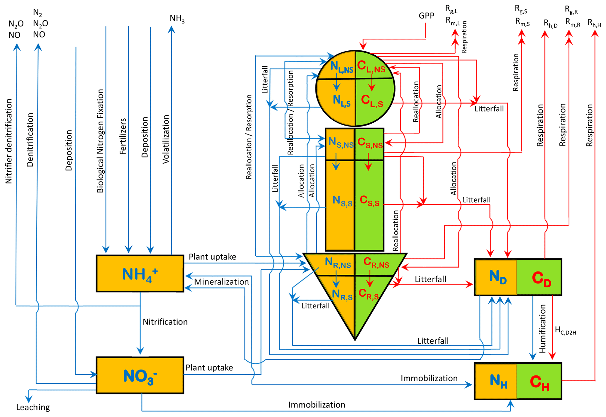
Figure 1The structure of the CLASSIC model used in this study. The 8 prognostic carbon pools are shown in a green colour, and carbon fluxes in a red colour. The 10 prognostic nitrogen pools are shown in an orange colour, and nitrogen fluxes are shown in a blue colour.
The individual terms of the rate change equations of the 10 prognostic N pools (Eqs. A1–A8, A10, and A11 in the Appendix), corresponding to Fig. 1, are specified or parameterized as explained in the following sections. These parameterizations are divided into three groups and related to (1) N inputs, (2) N cycling in vegetation and soil, and (3) N cycling in mineral pools and N outputs.
3.2 N inputs
3.2.1 Biological N fixation
Biological N fixation (BNF, ) is caused by both free-living bacteria in the soil and bacteria symbiotically living within nodules of host plants' roots. Here, the bacteria convert free nitrogen from the atmosphere to ammonium, which is used by the host plants. Like any other microbial activity, BNF is limited by both drier soil moisture conditions and cold temperatures. Cleveland et al. (1999) attempt to capture this by parameterizing BNF as a function of actual evapotranspiration (AET). AET is a function primarily of soil moisture (through precipitation and soil water balance) and available energy. In places where vegetation exists, AET is also affected by vegetation characteristics including the LAI and rooting depth. Here, we parameterize BNF (; ) as a function of modelled soil moisture and temperature to a depth of 0.5 m (following the use of a similar depth by Xu-Ri and Prentice, 2008) which yields a very similar geographical distribution of BNF as the approach of Cleveland et al. (1999) as seen later in Sect. 4.
where αc and αn () are BNF coefficients for crop (c) and non-crop or natural (n) PFTs, which are area weighted using the fractional coverages fc and fn of crop and non-crop PFTs that are present in a grid cell; f(T) is the dependence on soil temperature based on a Q10 formulation; and f(θ) is the dependence on soil moisture which varies between 0 and 1. θfc and θw are the soil moisture at field capacity and wilting points, respectively. T0.5 (∘C) and θ0.5 (m3 m−3) in Eq. (3) are averaged over the 0.5 m soil depth over which BNF is assumed to occur. We do not make the distinction between symbiotic and non-symbiotic BNF since this requires explicit knowledge of the geographical distribution of N-fixing PFTs which are not represented separately in our base set of nine PFTs. A higher value of αc is used compared to αn to account for the use of N-fixing plants over agricultural areas. Biological nitrogen fixation has been an essential component of many farming systems for considerable periods, with evidence for the agricultural use of legumes dating back more than 4000 years (O'Hara, 1998). A higher αc than αn is also consistent with Fowler et al. (2013), who report BNF of 58 and 60 Tg N yr−1 for natural and agricultural ecosystems for the present day. Since the area of natural ecosystems is about 5 times the current cropland area, this implies the BNF rate per unit land area is higher for crop ecosystems than for natural ecosystems. Values of αc than αn and other model parameters are summarized in Table A1.
Similarly to Cleveland et al. (1999), our approach does not lead to a significant change in BNF with increasing atmospheric CO2, other than through changes in soil moisture and temperature. At least two meta-analyses, however, suggest that an increase in atmospheric CO2 does lead to an increase in BNF through increased symbiotic activity associated with an increase in both nodule mass and number (McGuire et al., 1995; Liang et al., 2016). Models have attempted to capture this by simulating BNF as a function of NPP (Thornton et al., 2007; Wania et al., 2012). The caveat with this approach and the implications of our BNF approach are discussed in Sect. 6.
3.2.2 Atmospheric N deposition
Atmospheric N deposition is externally specified. The model reads from a file with spatially and temporally varying annual deposition rates. Deposition is assumed to occur at the same rate throughout the year, so the same daily rate () is used for all days of a given year. If separate information for ammonium () and nitrate () deposition rates is available, then it is used; otherwise deposition is assumed to be split equally between and (indicated as and in Eqs. A1 and A2).
3.2.3 Fertilizer application
Geographically and temporally varying annual fertilizer application rates () are also specified externally and read in. Fertilizer application occurs over the C3 and C4 crop fractions of grid cells. Agricultural management practices are difficult to model since they vary widely between countries and even from farmer to farmer. For simplicity, we assume fertilizer is applied at the same daily fertilizer application rate () throughout the year in the tropics (between 30∘ S and 30∘ N), given the possibility of multiple crop rotations in a given year. Between the 30∘ and 90∘ latitudes in both the Northern Hemisphere and the Southern Hemisphere, we assume that fertilizer application starts on the spring equinox and ends on the fall equinox. The annual fertilizer application rate is thus distributed over around 180 d. This provides somewhat greater realism than using the same treatment as in tropical regions, since extra-tropical agricultural areas typically do not experience multiple crop rotations in a given year. Prior knowledge of start and end days for fertilizer application makes it easier to figure out how much fertilizer is to be applied each day and helps ensure that the annual amount read from the externally specified file is consistently applied.
3.3 N cycling in plants and soil
Plant roots take up mineral N from soil and then allocate it to the leaves and stem to maintain an optimal C:N ratio of each component. Both active and passive plant uptakes of N (from both the and pools, explained in Sect. 3.3.2 and 3.3.3) are explicitly modelled. The active N uptake is modelled as a function of fine-root biomass, and passive N uptake depends on the transpiration flux. The modelled plant N uptake also depends on its N demand. Higher N demand leads to higher mineral N uptake from soil as explained below. Litterfall from vegetation contributes to the litter pool, and decomposition of litter transfers humified litter to the soil organic matter pool. Decomposition of litter and soil organic matter returns mineralized N back to the pool, closing the soil–vegetation N cycle loop.
3.3.1 Plant N demand
Plant N demand is calculated based on the fraction of NPP allocated to leaves, stem, and root components and their specified minimum PFT-dependent C:N ratios, similarly to other models (Xu-Ri and Prentice, 2008; Jiang et al., 2019). The assumption is that plants always want to achieve their desired minimum C:N ratios if enough N is available.
where the whole plant N demand (ΔWP) is the sum of the N demand for the leaves (ΔL), stem (ΔS), and root (ΔR) components; ai,C, is the fraction of NPP (i.e., carbon as indicated by letter C in the subscript; ) allocated to leaf, stem, and root components; and ratios, , are their specified minimum C:N ratios (see Table A1 for these and all other model parameters). A caveat with this approach when applied at the daily time step, for biogeochemical processes in our model, is that during periods of time when NPP is negative due to adverse climatic conditions (e.g., during winter or drought seasons), the calculated demand is negative. If positive NPP implies there is demand for N, negative NPP cannot be taken to imply that N must be lost from vegetation. As a result, from a plant's perspective, N demand is assumed to be zero during periods of negative NPP. N demand is also set to zero when all leaves have been shed (i.e., when GPP is zero). At the global scale, this leads to about a 15 % higher annual N demand than would be the case if negative NPP values were taken into consideration.
3.3.2 Passive N uptake
N demand is weighed against passive and active N uptake. Passive N uptake depends on the concentration of mineral N in the soil and the water taken up by the plants through their roots as a result of transpiration. We assume that plants have no control over N that comes into the plant through this pathway. This is consistent with existing empirical evidence that too much N in soil will cause N toxicity (Goyal and Huffaker, 1984), although we do not model N toxicity in our framework. If the N demand for the current time step cannot be met by passive N uptake, then a plant compensates for the deficit (i.e., the remaining demand) through active N uptake.
The concentration in the soil moisture within the rooting zone, referred to as [NH4] (gN gH2O−1), is calculated as
where is the ammonium pool size (gN m−2), θi is the volumetric soil moisture content for soil layer i (m3 m−3), zi is the thickness of soil layer i (m), and rI is the soil layer in which the 99 % rooting depth lies as dynamically simulated by the biogeochemical module of CLASSIC following Arora and Boer (2003). The 106 term converts units of the denominator term to gH2O m−2. The concentration ([NO3]; gN gH2O−1) in the rooting zone is found in a similar fashion. The transpiration flux qt () (calculated in the physics module of CLASSIC) is multiplied by [NH4] and [NO3] (gN gH2O−1) to obtain the passive uptake of and () as
where the multiplier 86 400×103 converts qt to units of and β (see Table A1) is the dimensionless mineral N distribution coefficient with a value of less than 1 that accounts for the fact that and available in the soil are not well mixed in the soil moisture solution to be taken up by plants and are not completely accessible to roots.
3.3.3 Active N uptake
The active plant N uptake is parameterized as a function of fine-root biomass and the size of and pools in a manner similar to Gerber et al. (2010) and Wania et al. (2012). The distribution of fine roots across the soil layers is ignored. CLASSIC does not explicitly model fine-root biomass. We therefore calculate the fraction of fine-root biomass using an empirical relationship that is very similar to the relationship developed by Kurz et al. (1996) (their Eq. 5) but also works below a total root biomass of 0.33 kg C m−2 (the relationship of Kurz et al. (1996) yields a fraction of fine-root biomass of more than 1.0 below this threshold). The fraction of fine-root biomass (fr) is given by
where CR is the root biomass (kg C m−2) simulated by the biogeochemical module of CLASSIC. Equation (7) yields a fine-root fraction approaching 1.0 as CR approaches 0, so at very low root biomass values all roots are considered fine roots. For grasses the fraction of fine-root biomass is set to 1. The maximum or potential active N uptake for and is given by
where ε (see Table A1) is the efficiency of fine roots to take up N per unit fine-root mass per day (), (see Table A1) is the half-saturation constant (gN m−3), rd is the 99 % rooting depth (m), and and are the ammonium and nitrate pool sizes (gN m−2) as mentioned earlier. Depending on the geographical location and the time of the year, if passive uptake alone can satisfy plant N demand, the actual active N uptake of () and () is set to zero. Conversely, during other times both passive and potential active N uptakes may not be able to satisfy the demand, and in this case actual active N uptake is equal to its potential rate. At times other than these, the actual active uptake is lower than its potential value. This adjustment of actual active uptake is illustrated in Eq. (9).
Finally, the total N uptake (U), uptake of (), and () are calculated as
3.3.4 Litterfall
Nitrogen litterfall from the vegetation components is directly tied to the carbon litterfall calculated by the phenology module of CLASSIC through their current C:N ratios.
where LFi,C is the carbon litterfall rate (gC d−1) for component i, calculated by the phenology module of CLASSIC, and division by its current C:N ratio yields the nitrogen litterfall rate; rL (see Table A1) is the leaf resorption coefficient that simulates the resorption of N from leaves of deciduous-tree PFTs before they are shed; and ri=0, for . Litter from each vegetation component is proportioned between structural and non-structural components according to their pool sizes.
3.3.5 Allocation and reallocation
Plant N uptake by roots is allocated to leaves and stem to satisfy their N demand. When plant N demand is greater than zero, total N uptake (U) is divided between leaves, stem, and root components in proportion to their demands such that the allocation fractions for N (ai, ) are calculated as
where AR2L and AR2S are the amounts of N allocated from root to leaves and stem components, respectively, as shown in Eqs. (A5) and (A7). During periods of negative NPP due to adverse climatic conditions (e.g., during winter or drought seasons) the plant N demand is set to zero but passive N uptake, associated with transpiration, may still be occurring if the leaves are still on. Even though there is no N demand, passive N uptake still needs to be partitioned among the vegetation components. During periods of negative NPP, allocation fractions for N are, therefore, calculated in proportion to the minimum PFT-dependent C:N ratios of the leaves, stem, and root components as follows:
For grasses, which do not have a stem component, Eqs. (12) and (13) are modified accordingly by removing the terms associated with the stem component.
Three additional rules override these general allocation rules specifically for deciduous-tree PFTs (or deciduous PFTs in general). First, no N allocation is made to leaves once leaf fall is initiated for deciduous-tree PFTs, and plant N uptake is proportioned between stem and root components based on their demands in a manner similar to Eq. (12). Second, for deciduous-tree PFTs, a fraction of leaf N is resorbed from leaves back into the stem and roots as follows:
where rL is the leaf resorption coefficient, as mentioned earlier, and LFL is the leaf litterfall rate. Third, and similar to resorption, at the time of leaf onset for deciduous-tree PFTs, N is reallocated to leaves (in conjunction with reallocated carbon as explained in Asaadi et al., 2018) from stem and root components.
where RR2L,C and RS2L,C represent the reallocation of carbon from non-structural stem and root components to leaves and division by C:NL converts the flux into N units. This reallocated N, at the time of leaf onset, is proportioned between non-structural pools of the stem and roots according to their sizes.
3.3.6 N mineralization, immobilization, and humification
Decomposition of litter (Rh,D) and soil organic matter (Rh,H) releases C to the atmosphere, and this flux is calculated by the heterotrophic respiration module of CLASSIC. The litter and soil carbon decomposition rates used here are the same as in the standard model version (Melton and Arora, 2016, their Table A3). The amount of N mineralized is calculated straightforwardly by division with the current C:N ratios of the respective pools and contributes to the pool.
An implication of mineralization contributing to the pool, in addition to BNF and fertilizer inputs that also contribute solely to the pool, is that the simulated pool is typically larger than the pool. The exception is the dry and arid regions where the lack of denitrification, as discussed below in Sect. 3.4.2, leads to a buildup of the pool.
Immobilization of mineral N from the and pools into the soil organic matter pool is meant to keep the soil organic matter C:N ratio (C:NH) at its specified value of 13 for all PFTs in a manner similar to Wania et al. (2012) and Zhang et al. (2018). A value of 13 is within the range of observation-based estimates which vary from about 8 to 25 (Zinke et al., 1998; Tipping et al., 2016). Although C:NH varies geographically, the driving factors behind this variability remain unclear. It is even more difficult to establish if increasing atmospheric CO2 is changing C:NH given the large heterogeneity in soil organic C and N densities and the difficulty in measuring small trends for such large global pools. We therefore make the assumption that the C:NH ratio does not change with time. An implication of this assumption is that as GPP increases with increasing atmospheric CO2 rises and plant litter becomes enriched in C with an increasing C:N ratio of litter, more and more N is locked up in the soil organic matter pool because its C:N ratio is fixed. As a result, mineral N pools of and decrease in size and the plant N amount subsequently follows. This is consistent with studies of plants grown in elevated-CO2 environments. For example, Cotrufo et al. (1998) summarize results from 75 studies and find an average 14 % reduction in N concentration (gN∕gC) for aboveground tissues. Wang et al. (2019) find increased C concentration by 0.8 %–1.2 % and a reduction in N concentration by 7.4 %–10.7 % for rice and winter wheat crop rotation systems under elevated CO2. Another implication of using a specified fixed C:NH ratio is that it does not matter if plant N uptake or immobilization is given preferred access to the mineral N pool since in the long term, by design, N will accumulate in the soil organic matter in response to an atmospheric CO2 increase.
Immobilization from both the and the pools () is calculated in proportion to their pool sizes, employing the fixed C:NH ratio as
where kO is rate constant with a value of 1.0 d−1. Finally, the carbon flux of humified litter from the litter to the soil organic matter pool (HC,D2H) is also associated with a corresponding N flux that depends on the C:N ratio of the litter pool.
3.4 N cycling in mineral pools and N outputs
This section presents the parameterizations of nitrification (which results in transfer of N from the to the pool) and the associated gaseous fluxes of N2O and NO (referred to as nitrifier denitrification); gaseous fluxes of N2O, NO, and N2 associated with denitrification; volatilization of into NH3; and leaching of in runoff.
3.4.1 Nitrification
Nitrification, the oxidative process converting ammonium to nitrate, is driven by microbial activity and as such is constrained by both high and low soil moisture (Porporato et al., 2003). At high soil moisture content there is little aeration of soil, and this constrains aerobic microbial activity, while at low soil moisture content microbial activity is constrained by moisture limitation. In CLASSIC, the heterotrophic respiration from soil carbon is constrained similarly, but rather than using soil moisture the parameterization is based on soil matric potential (Arora, 2003; Melton et al., 2015). Here, we use the exact same parameterization. In addition to soil moisture, nitrification () is modelled as a function of soil temperature and the size of the pool as follows:
where η is the nitrification coefficient (d−1; see Table A1); fI(ψ) is the dimensionless soil moisture scalar that varies between 0 and 1 and depends on soil matric potential (ψ); fI(T0.5) is the dimensionless soil temperature scalar that depends on soil temperature (T0.5) averaged over the top 0.5 m soil depth over which nitrification is assumed to occur (following Xu-Ri and Prentice, 2008); and is the ammonium pool size (gN m−2), as mentioned earlier. Both fI(T0.5) and fI(ψ) are parameterized following Arora (2003) and Melton et al. (2015). fI(T0.5) is a Q10-type function with a temperature-dependent Q10:
The reference temperature for nitrification is set to 20 ∘C following Lin et al. (2000). fI(ψ) is parameterized as a step function of soil matric potential (ψ) as
where the soil matric potential (ψ) is found, following Clapp and Hornberger (1978), as a function of soil moisture (θ):
The saturated matric potential (ψsat), soil moisture at saturation (i.e., porosity) (θsat), and the parameter B are calculated as functions of percent sand and clay in soil following Clapp and Hornberger (1978) as shown in Melton et al. (2015). The soil moisture scalar fI(ψ) is calculated individually for each soil layer and then averaged over the soil depth of 0.5 m over which nitrification is assumed to occur.
Gaseous fluxes of NO (INO) and N2O () associated with nitrification and generated through nitrifier denitrification are assumed to be directly proportional to the nitrification flux () as
where ηNO and are dimensionless fractions (see Table A1) which determine what fractions of nitrification flux are emitted as NO and N2O.
3.4.2 Denitrification
Denitrification is the stepwise microbiological reduction in nitrate to NO, to N2O, and ultimately to N2 in complete denitrification. Unlike nitrification, however, denitrification is primarily an anaerobic process (Tomasek et al., 2017) and therefore occurs when soil is saturated. As a result, we use a different soil moisture scalar than for nitrification. Similar to nitrification, denitrification is modelled as a function of soil moisture, soil temperature, and the size of the pool as follows to calculate the gaseous fluxes of NO, N2O, and N2.
where μNO, , and are coefficients (d−1; see Table A1) that determine daily rates of emissions of NO, N2O, and N2. The temperature scalar fE(T0.5) is exactly the same as the one for nitrification (fI(T0.5)) since denitrification is also assumed to occur over the same 0.5 m soil depth. The soil moisture scalar fE(θ) is given by
where w is the soil wetness that varies between 0 and 1 as soil moisture varies between the wilting point (θw) and field capacity (θf) and wd (see Table A1) is the threshold soil wetness for denitrification below which very little denitrification occurs. Since arid regions are characterized by low soil wetness values, typically below wd, this leads to the buildup of the pool in arid regions.
3.4.3 leaching
Leaching is the loss of water-soluble ions through runoff. In contrast to positively charged ions (i.e., cations), the ions do not bond to soil particles because of the limited exchange capacity of soil for negatively charged ions (i.e., anions). As a result, leaching of N in the form of ions is a common water quality problem, particularly over cropland regions. The leaching flux (; ) is parameterized to be directly proportional to the baseflow (bt; ) calculated by the physics module of CLASSIC and the size of the pool (; gN m−2). The baseflow is the runoff rate from the bottommost soil layer.
where the multiplier 86 400 converts units to per day and φ is the leaching coefficient (m2 kg−1; see Table A1) that can be thought of as the soil particle surface area (m2) that 1 kg of water (or about 0.001 m3) can effectively wash to leach the nutrients.
3.4.4 NH3 volatilization
NH3 volatilization (; ) is parameterized as a function of the pool size of , soil temperature, soil pH, aerodynamic and boundary layer resistances, and atmospheric NH3 concentration in a manner similar to Riddick et al. (2016) as
where ϑ is the dimensionless NH3 volatilization coefficient (see Table A1) which is set to less than 1 to account for the fact that a fraction of ammonia released from the soil is captured by vegetation; ra (s m−1) is the aerodynamic resistance calculated by the physics module of CLASSIC; χ is the ammonia (NH3) concentration at the interface of the top soil layer and the atmosphere (g m−3); [NH3,a] is the atmospheric NH3 concentration specified at g m−3 following Riddick et al. (2016); 86 400 converts flux units from to ; and rb (s m−1) is the boundary layer resistance calculated following Thom (1975) as
where u* (m s−1) is the friction velocity provided by the physics module of CLASSIC. The ammonia (NH3) concentration at surface (χ), in a manner similar to Riddick et al. (2016), is calculated as
where the coefficient 0.26 is the fraction of ammonium in the top 10 cm soil layer assuming the exponential distribution of ammonium along the soil depth (given by 3e−3z, where z is the soil depth), KH (dimensionless) is the Henry's law constant for NH3, (mol L−1) is the dissociation equilibrium constant for aqueous NH3, and H+ (mol L−1) is the concentration of hydrogen ion that depends on the soil pH (). KH and are modelled as functions of the soil temperature of the top 10 cm soil layer (T0.1) following Riddick et al. (2016) as
where Tref,v is the reference temperature of 298.15 K.
3.5 Coupling of C and N cycles
As mentioned earlier, the primary objective of the coupling of C and N cycles is to be able to simulate Vcmax as a function of leaf N amount (NL; gN m−2 land) for each PFT. This coupling is represented through the following relationship:
where Γ1 (39 ) and Γ2 (8.5 ) are global constants, except for the broadleaf-evergreen-tree PFT for which a lower value of Γ1 (15.3 ) is used as discussed below, and the number 3 represents an average LAI over vegetated areas (m2 of leaves∕m2 of land). Λ (≤1) is a scalar that reduces the calculated Vcmax when the C:N ratio of any plant component exceeds its specified maximum value ( (see Table A1).
where kΛ is a dimensionless parameter (see Table A1) and ω is a dimensionless term that represents excess C:N ratios above specified maximum thresholds weighted by . When plant components do not exceed their specified maximum C:N ratio thresholds, ei is zero and Λ is 1. When plant components exceed their specified maximum C:N ratio thresholds, Λ starts reducing to below 1. This decreases Vcmax and thus photosynthetic uptake which limits the rate of increase in the C:N ratio of plant components, depending on the value of kΛ.
The linear relationship between photosynthetic capacity and NL (Evans, 1989; Field and Mooney, 1986; Garnier et al., 1999) (used in Eq. 31) and between photosynthetic capacity and leaf chlorophyll amount (Croft et al., 2017) is empirically observed. We have avoided using PFT-dependent values of Γ1 and Γ2 not only for the easy optimization of these parameter values but also because such an optimization can potentially hide other model deficiencies. More importantly, using PFT-independent values of Γ1 and Γ2 yields a more elegant framework, whose successful evaluation will provide confidence in the overall model structure.
As shown later in the “Results” section, using Γ1 and Γ2 as global constants yields GPP values that are higher in the tropical region than those given by an observation-based estimate. This is not surprising since tropical and mid-latitude regions are known to be limited by P (Vitousek, 1984; Aragão et al., 2009; Vitousek et al., 2010; Du et al., 2020) and our framework currently does not model the P cycle explicitly. An implication of productivity that is limited by P is that changes in NL are less important. In the absence of the explicit treatment of the P cycle, we therefore simply use a lower value of Γ1 for the broadleaf-evergreen-tree PFT which, in our modelling framework, exclusively represents a tropical PFT. Although it is a simple way to express P limitation, this approach yields the best comparison with observation-based GPP, as shown later, because the effect of P limitation is most pronounced in the high-productivity tropical regions.
The second pathway of coupling between the C and N cycles occurs through the mineralization of litter and soil organic matter. During periods of higher temperature, heterotrophic C respiration fluxes increase from the litter and soil organic matter pools, and this in turn implies an increased mineralization flux (via Eq. 16), leading to more mineral N available for plants to uptake.
4.1 Model simulations and input data sets
We perform CLASSIC model simulations with the N cycle for the pre-industrial period followed by several simulations for the historical 1851–2017 period to evaluate the model's response to different forcings, as summarized below. The simulation for the pre-industrial period uses forcings that correspond to the year 1850, and the model is run for thousands of years until its C and N pools come into equilibrium. Global thresholds of the net atmosphere–land C flux of 0.05 Pg yr−1 and the net atmosphere–land N flux of 0.5 Tg N yr−1 are used to ensure the model pools have reached equilibrium. The pre-industrial simulation, therefore, yields the initial conditions from which the historical simulations for the period 1851–2017 are launched. To spin up the mineral N pools to their initial values, the plant N uptake and other organic processes were turned off while the model used specified values of Vcmax and only the inorganic part of the N cycle was operative. Once the inorganic mineral soil N pools reached near equilibrium, the organic processes were turned on. The model also uses an accelerated spin-up procedure for the slow pools of soil organic matter and mineral N. The input and output terms are multiplied by a factor of greater than 1, and this magnifies the change in pool size and therefore accelerates the spin-up. Once the model pools reach near equilibrium, the factor is set back to 1.
Table 1Historical simulations performed over the period 1851–2017 to evaluate the model's response to various forcings. All forcings are time varying. All forcings are also spatially explicit except atmospheric CO2, for which a globally constant value is specified.
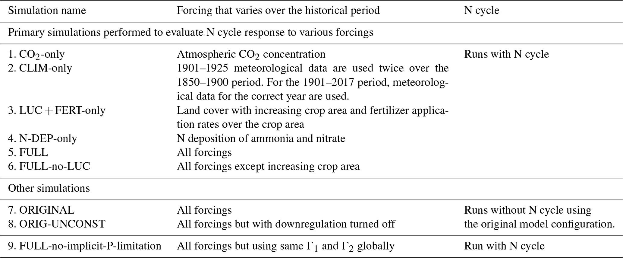
To evaluate the model's response to various forcings over the historical period, we perform several simulations turning on one forcing at a time as summarized in Table 1. The objective of these simulations is to see if the model response to individual forcings is consistent with expectations. For example, in the CO2-only simulation only the atmospheric CO2 concentration increases over the historical period while all other forcings stay at their 1850 levels. In the N-DEP-only simulation only the N deposition increases over the historical period, and similarly for other runs in Table 1. A “FULL” simulation with all forcings turned on is then also performed which we compare to the original model without a N cycle which uses the photosynthesis downregulation parameterization (termed “ORIGINAL” in Table 1). Finally, a separate pre-industrial simulation is also performed that uses the same Γ1 and Γ2 globally (FULL-no-implicit-P-limitation). This simulation is used to illustrate the effect of neglecting P limitation for the broadleaf-evergreen-tree PFT in the tropics.
For the historical period, the model is driven with time-varying forcings that include CO2 concentration, population density (used by the fire module of the model for calculating anthropogenic fire ignition and suppression), land cover, and meteorological data. In addition, for the N-cycle module, the model requires time-varying atmospheric N deposition and fertilizer data. The atmospheric CO2 and meteorological data (CRU-JRA) are the same as those used for the TRENDY model intercomparison project for terrestrial ecosystem models for the year 2018 (Le Quéré et al., 2018). The CRU-JRA meteorological data are based on 6-hourly Japanese Reanalysis (JRA). However, since reanalysis data typically do not match observations, their monthly values are adjusted based on the Climatic Research Unit (CRU) data. This yields a blended product with a sub-daily temporal resolution that comes from the reanalysis and monthly means and sums that match the CRU data to yield a meteorological product that can be used by models that require sub-daily or daily meteorological forcing. These data are available for the period 1901–2017. Since no meteorological data are available for the 1850–1900 period, we use 1901–1925 meteorological data repeatedly for this duration and also for the pre-industrial spin-up. The assumption is that since there is no significant trend in the CRU-JRA data over this period, these data can be reliably used to spin up the model to equilibrium. The land cover data used to force the model are based on a geographical reconstruction of the historical land cover driven by the increase in crop area following Arora and Boer (2010) but using the crop area data prepared for the Global Carbon Project (GCP) 2018 following Hurtt et al. (2020). Since land cover is prescribed, the competition between PFTs for space for the simulations reported here is switched off. The population data for the period 1850–2017 are based on Klein Goldewijk et al. (2017) and obtained from ftp://ftp.pbl.nl/../hyde/hyde3.2/baseline/zip/ (last access: July 2018). The time-independent forcings consist of soil texture and soil permeable-depth data.
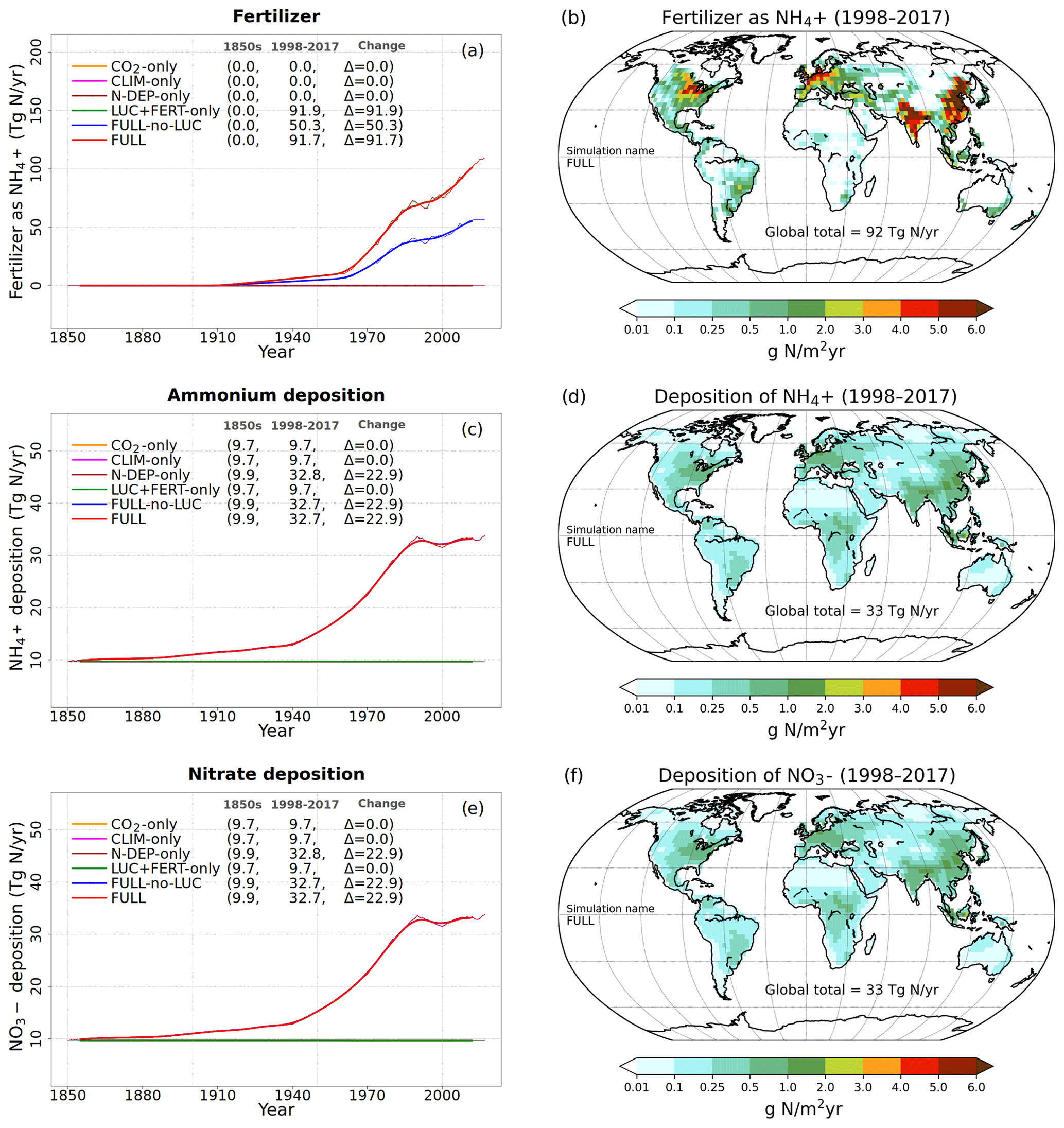
Figure 2Time series and geographical distribution of global annual values of externally specified N inputs. Fertilizer input (a, b), atmospheric deposition of ammonium (c, d), and atmospheric deposition of nitrate (e, f). The values in the parentheses for legend entries show the average for the 1850s, the average for the 1998–2017 period, and the change between them. The thin lines in the time series plots show the annual values, and the thick lines show their 10-year moving average. The geographical plots show the average values over the last 20 years of the FULL simulation corresponding to the 1998–2017 period. Note that in the time series plots, lines from some simulations are hidden behind lines from other simulations, and this can be inferred from the legend entries which show averages for the 1850s and the 1998–2017 period.
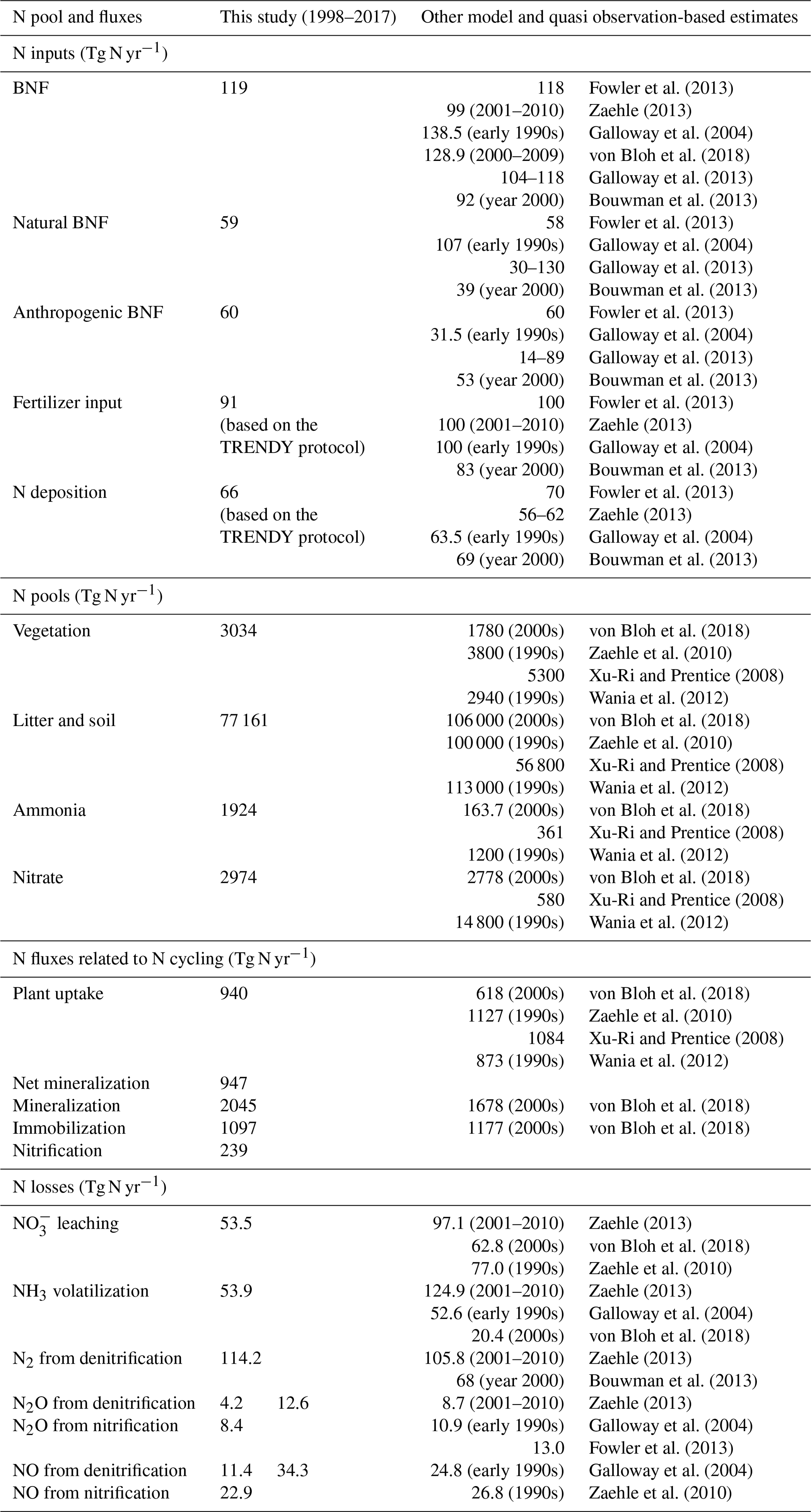
Table 2Comparison of simulated global N pools and fluxes, from the FULL simulation, with other modelling and quasi observation-based studies (references for which are noted in the table). The time periods to which the other modelling and quasi observation-based estimates correspond are also noted, where available. The estimates are for land. The simulated fluxes and pool correspond to the period 1997–2018. In the last few rows, the simulated N2O and NO emissions from denitrification and nitrification are reported separately but also as their combined total. For these N2O and NO emissions, it is the combined total that must be compared to other estimates.
Time-varying atmospheric-N-deposition and fertilizer data used over the historical period are also specified as per the TRENDY protocol. The fertilizer data are based on the N2O model intercomparison project (NMIP) (Tian et al., 2018) and available for the period 1860–2014. For the period before 1860, 1860 fertilizer application rates are used. For the period after 2014, fertilizer application rates for 2014 are used. Atmospheric-N-deposition data are from input4MIPs (https://esgf-node.llnl.gov/search/input4mips/, last access: 28 April 2020) and are the same as those used by models participating in CMIP6 for the historical period (1850–2014). For the years 2015–2017 the N deposition data corresponding to those from the representative concentration pathway (RCP) 8.5 scenario are used. Figure 2 shows the time series of global annual values of externally specified fertilizer input and of deposition of ammonium and nitrate, based on the TRENDY protocol, for the six primary simulations. The geographical distribution of these inputs is also shown for the last 20 years from the FULL simulation corresponding to the 1998–2017 period. In Fig. 2a, c, and e ammonium and nitrate deposition and fertilizer input stay at their pre-industrial level for simulations in which these forcings do not increase over the historical period. As mentioned earlier, N deposition is split evenly into ammonium and nitrate. The values in parentheses in the Fig. 2a legend and in subsequent time series plots show average values over the 1850s and over the last 20 years (1998–2017) of the simulations, and the change between these two periods. The present-day values of fertilizer input and N deposition are consistent with other estimates available in the literature (Table 2). The fertilizer input rate in the simulation with all forcings except land use change (FULL-no-LUC, blue line), that is with no increase in crop area over its 1850 value, is 50 Tg N yr−1 compared to 91 Tg N yr−1 in the FULL simulation, averaged over the 1998–2017 period. The additional 41 Tg N yr−1 of fertilizer input occurs in the FULL simulation not only due to the increase in crop area but also due to the increasing fertilizer application rates over the historical period. The geographical distribution of the fertilizer application rates in Fig. 2b shows that they are concentrated in regions with crop areas and have values as high as 16 especially in eastern China. The N deposition rates (Fig. 2d and f) are more evenly distributed geographically than the fertilizer applications rates, as would be expected, since emissions are transported downstream from their point sources. Areas with high emissions like the eastern United States, India, eastern China, and Europe, however, still stand out as areas that receive higher N deposition.
4.2 Evaluation data sources
We compare globally summed annual values of N pools and fluxes with observations and other models and where available their geographical distribution and seasonality. In general, however, fewer observation-based data are available to evaluate simulated terrestrial N-cycle components than for C-cycle components. As a result, N pools and fluxes are primarily compared to results from both observation-based studies and other modelling studies (Bouwman et al., 2013; Fowler et al., 2013; Galloway et al., 2004; Vitousek et al., 2013; Zaehle, 2013). Since the primary purpose of the N cycle in our framework is to constrain the C cycle, we also compare globally summed annual values of GPP and the net atmosphere–land CO2 flux and their zonal distribution with available observation-based estimates and other estimates. The observation-based estimate of GPP is from Beer et al. (2010), who apply diagnostic models to extrapolate ground-based carbon flux tower observations from about 250 stations to the global scale. The observation-based net atmosphere–land CO2 flux is from Global Carbon Project's 2019 assessment (Friedlingstein et al., 2019).
5.1 N inputs – biological N fixation
Figure 3a, c, and e show the time series of annual values of BNF and its natural and anthropogenic components from the six primary simulations summarized in Table 1. BNF stays at its pre-industrial value of around 80 Tg N yr−1 in the CO2-only and N-DEP-only simulations. In the CLIM-only (indicated by a magenta-coloured line) and the FULL-no-LUC (blue line) simulations the change in climate, associated with increases in temperature and precipitation over the 1901–2017 period (see Fig. A2 in the Appendix), increases BNF to about 85 Tg N yr−1. In our formulation (Eq. 3) BNF is positively impacted by increases in temperature and precipitation. In the LUC + FERT-only simulation (dark-green line) the increase in crop area contributes to an increase in global BNF with a value of around 110 Tg N yr−1 for the present day, since a higher BNF per unit crop area is assumed than for natural vegetation. Finally, in the FULL simulation (red line) the 1998–2017 average value is around 117 Tg N yr−1 due to both changes in climate over the historical period and the increase in crop area. Our present-day value of global BNF is broadly consistent with other modelling and data-based studies as summarized in Table 2. Panels c and e in Fig. 3 show the separation of the total terrestrial BNF into its natural (over non-crop PFTs) and anthropogenic (over C3 and C4 crop PFTs) components. The increase in crop area over the historical period decreases natural BNF from its pre-industrial value of 59 to 54 Tg N yr−1 for the present day as seen for the LUC + FERT-only simulation (green line) in Fig. 3c, while anthropogenic BNF over agricultural areas increases from 21 to 56 Tg N yr−1 (Fig. 3e). Figure 3c and e show that the increase in BNF (Fig. 3a) in the FULL simulation is caused primarily by an increase in crop area. Our present-day values of natural and anthropogenic BNF are also broadly consistent with other modelling and data-based studies as summarized in Table 2.
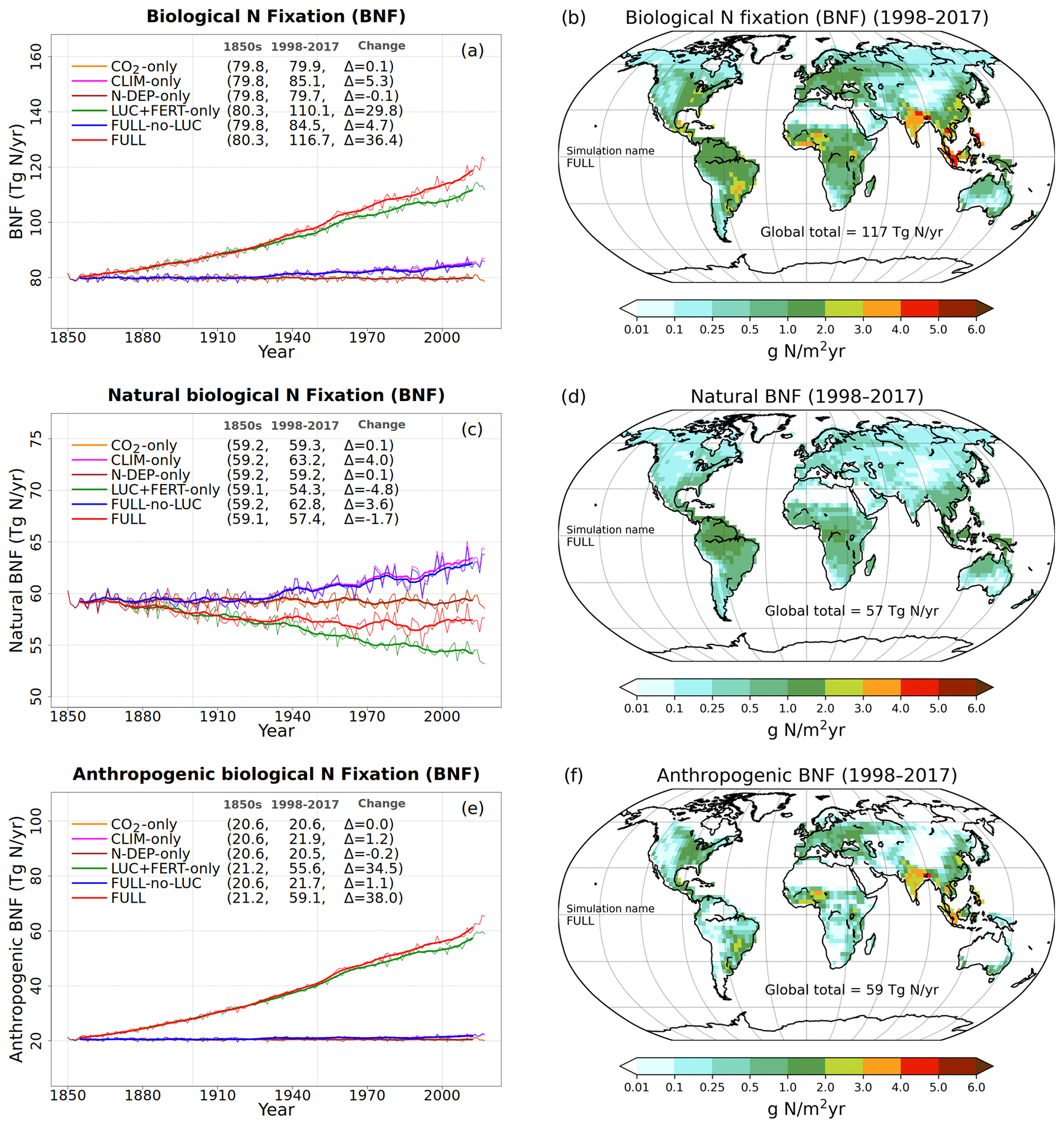
Figure 3Time series and geographical distribution of annual values of biological N fixation (BNF) (a, b) and its natural (c, d) and anthropogenic (e, f) components. The values in the parentheses for legend entries show the average for the 1850s, the average for the 1998–2017 period, and the change between them. The thin lines in the time series plots show the annual values, and the thick lines show their 10-year moving average. The geographical plots show the average values over the last 20 years of the FULL simulation corresponding to the 1998–2017 period. Note that in the time series plots, lines from some simulations are hidden behind lines from other simulations, and this can be inferred from the legend entries which show averages for the 1850s and the 1998–2017 period.
Figure 3b, d, and f show the geographical distribution of simulated BNF and its natural and anthropogenic components. The geographical distribution of BNF (Fig. 3a) looks very similar to the current distribution of vegetation (not shown) with warm and wet regions showing higher values than cold and dry regions since BNF is parameterized as a function of soil temperature and soil moisture. Anthropogenic BNF only occurs in regions where crop areas exist according to the specified land cover, and it exhibits higher values than natural BNF in some regions because of its higher value per unit area (see Sect. 3.2.1).
At the global scale and for the present day, natural BNF (59 Tg N yr−1) is overwhelmed by anthropogenic sources: anthropogenic BNF (60 Tg N yr−1), fertilizer input (91.7 Tg N yr−1), and atmospheric N deposition have increased since the pre-industrial era (∼45 Tg N yr−1). Currently humanity fixes more N than natural processes do (Vitousek, 1994).
5.2 C and N pools and flux responses to historical changes in forcings
To understand the model response to changes in various forcings over the historical period, we first look at the evolution of global values of primary C and N pools and fluxes, shown in Figs. 4 to 8. Figure 4a shows the time evolution of global annual GPP values, the primary flux of C into the land surface, for the six primary simulations, the ORIGINAL simulation performed with the model version with no N cycle, and the ORIG-UNCONST simulation with no photosynthesis downregulation (see Table 1). The unconstrained increase in GPP (35.6 Pg C yr−1 over the historical period) in the ORIG-UNCONST simulation (dark-cyan line) is governed by the standard photosynthesis model equations following Farquhar et al. (1980) and Collatz et al. (1992) for C3 and C4 plants, respectively. Downregulation of photosynthesis in the ORIGINAL simulation (purple line) is modelled on the basis of Eq. (1), while in the FULL simulation (red line) photosynthesis downregulation results from a decrease in Vcmax values (Fig. 5d) due to a decrease in the leaf N amount (Fig. 5b). We will compare the FULL and ORIGINAL simulations in more detail later. The simulations with individual forcings, discussed below, provide insight into the combined response of GPP to all forcings in the FULL simulation.
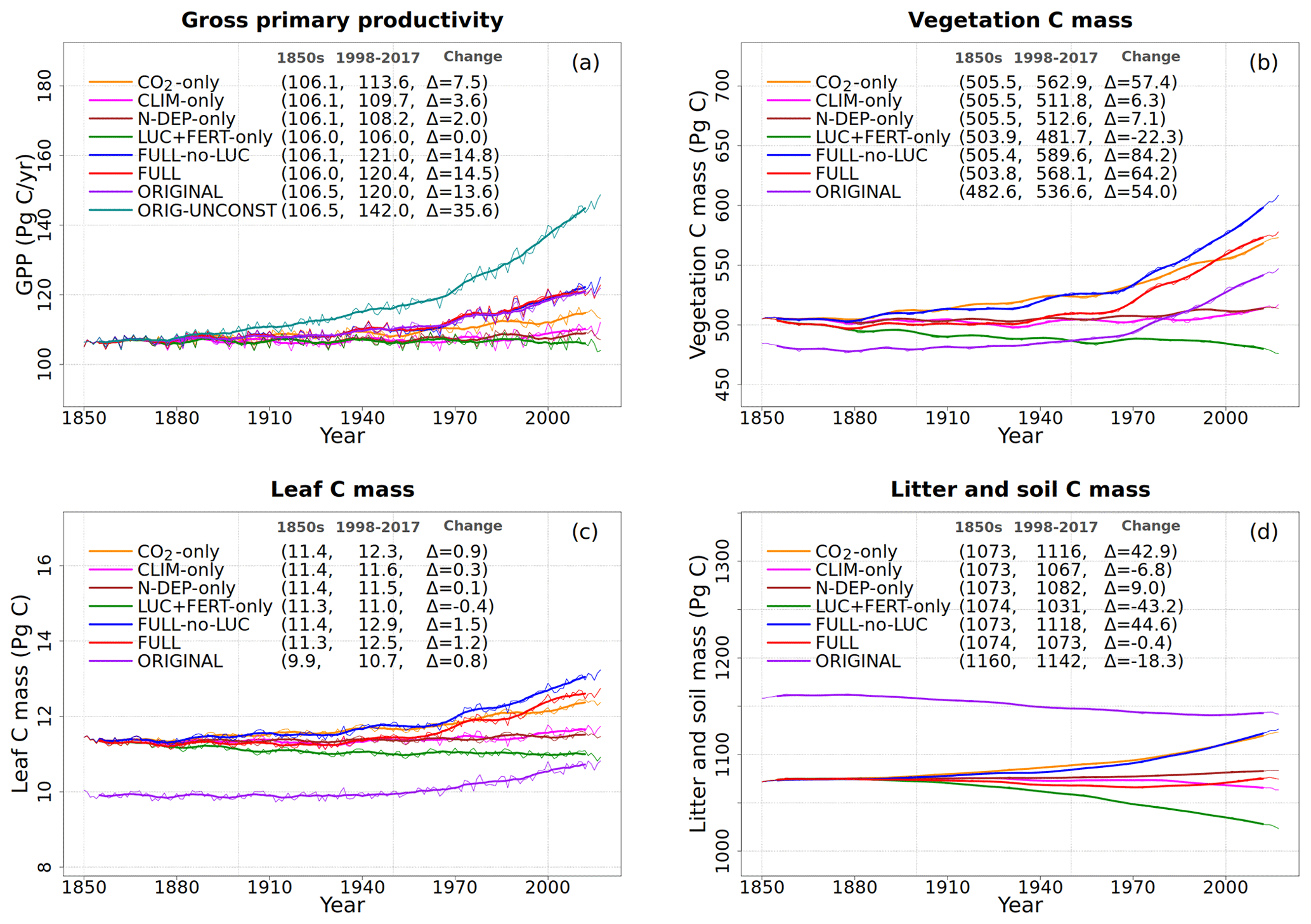
Figure 4Global annual values of gross primary productivity (a), vegetation carbon (b), leaf carbon (c), and litter and soil carbon (d) for the primary simulations performed. The values in the parentheses for legend entries show the average for the 1850s, the average for the 1998–2017 period, and the change between them. The thin lines show the annual values, and the thick lines show their 10-year moving average.
5.2.1 Response to increasing CO2
The response of C and N cycles to increasing CO2 in the CO2-only simulation (orange lines in Fig. 4) is the most straightforward to interpret. A CO2 increase causes GPP to increase by 7.5 Pg C yr−1 above its pre-industrial value (Fig. 4a), which in turn causes vegetation (Fig. 4b), leaf (Fig. 4c), and soil (Fig. 4d) carbon mass to increase as well. The vegetation and leaf N amounts (orange line, Fig. 5a and b), in contrast, decrease in response to increasing CO2. This is because N becomes locked up in the soil organic matter pool (Fig. 5c) in response to an increase in the soil C mass (due to the increasing GPP), litter inputs which are now rich in C (due to CO2 fertilization) but poor in N (since N inputs are still at their pre-industrial level), and the fact that the C:N ratio of the soil organic matter is fixed at 13. This response to elevated CO2 which leads to increased C and decreased N in vegetation is consistent with meta-analysis of 75 field experiments of elevated CO2 (Cotrufo et al., 1998). A decrease in N in leaves (orange line, Fig. 5b) leads to a concomitant decrease in the maximum carboxylation capacity (Vcmax) (orange line, Fig. 5d), and as a result GPP increases at a much slower rate in the CO2-only simulation than in the ORIG-UNCONST simulation (Fig. 4a). Due to the N accumulation in the soil organic matter pool, the and (Fig. 5e and f) pools also decrease in size in the CO2-only simulation.
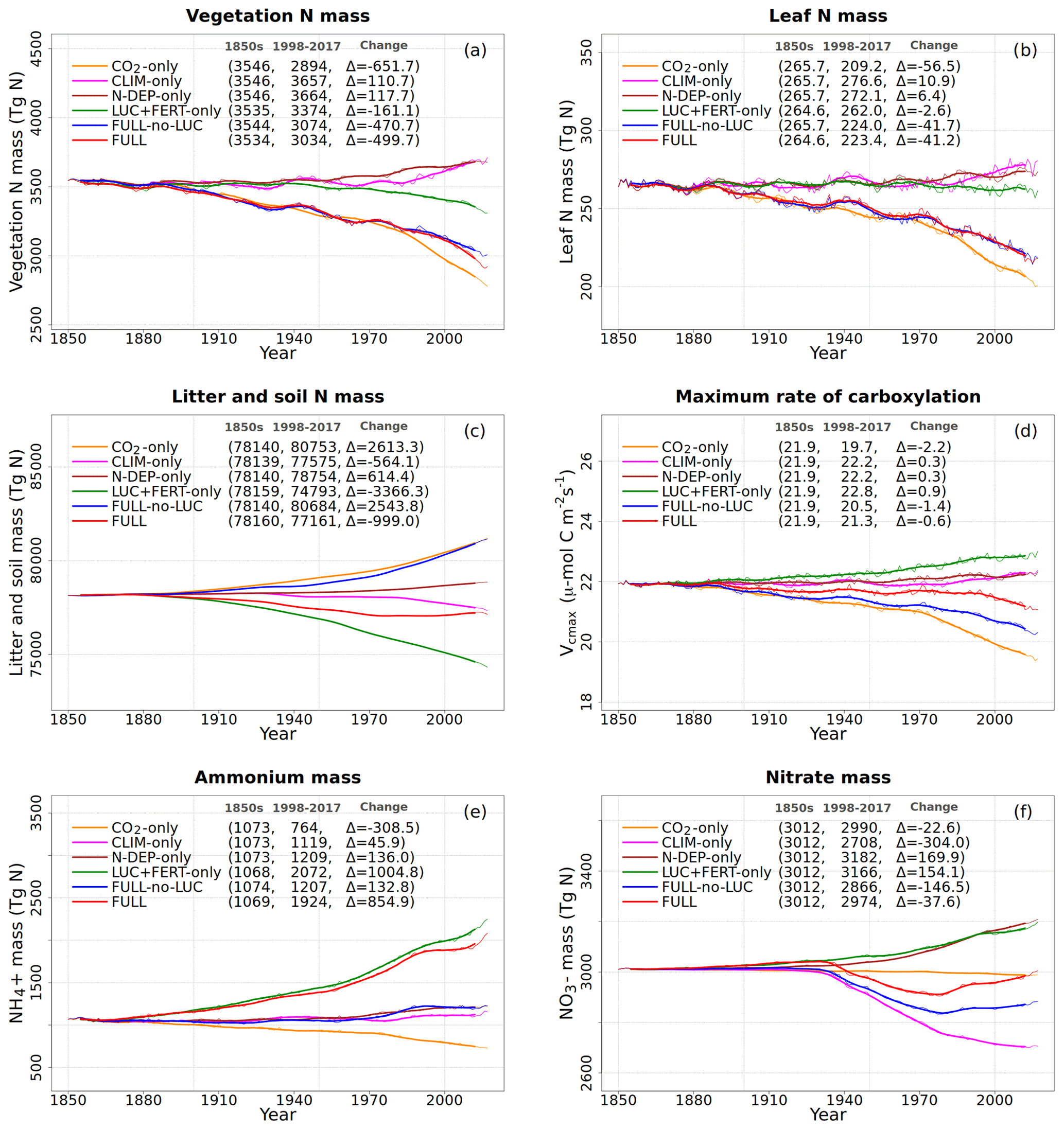
Figure 5Global annual values of N in vegetation (a), leaves (b), litter and soil organic matter (c) pools, Vcmax (d), and ammonium (e) and nitrate (f) pools for the primary simulations performed. The values in the parentheses for legend entries show the average for the 1850s, the average for the 1998–2017 period, and the change between them. The thin lines show the annual values, and the thick lines show their 10-year moving average.
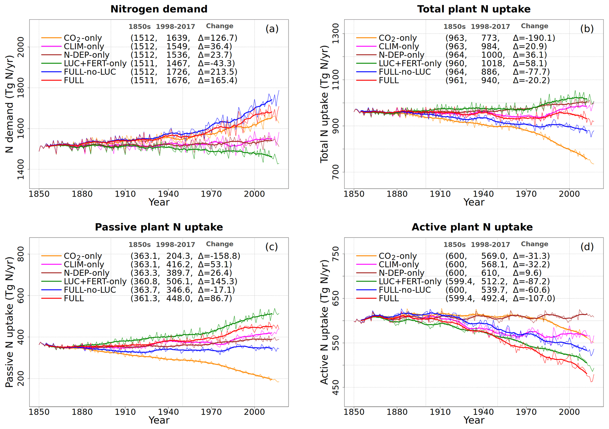
Figure 6Global annual values of N demand (a), total plant N uptake (b), and its split into passive (c) and active (d) components for the primary simulations performed. The values in the parentheses for legend entries show the average for the 1850s, the average for the 1998–2017 period, and the change between them. The thin lines show the annual values, and the thick lines show their 10-year moving average.
Figure 6 shows the time series of N demand, plant N uptake, and its split between passive and active N uptakes. The plant N demand in the CO2-only simulation (Fig. 6a, orange line) increases from its pre-industrial value of 1512 to 1639 Tg N yr−1 for the present day since the increasing C input from increasing GPP requires a higher N input to maintain the preferred minimum C:N ratio of plant tissues. However, since mineral N pools decrease in size over the historical period in this simulation (Fig. 5e and f), the total plant N uptake (Fig. 6b) reduces. Passive plant N uptake is directly proportional to pool sizes of and , and therefore it reduces in response to increasing CO2. Active plant N uptake, which compensates for insufficient passive N uptake compared to the N demand, also eventually starts to decline as it also depends on mineral N pool sizes. The eventual result of increased C supply and reduced N supply is an increase in the C:N ratio of all plant components and litter (Fig. 7). The pre-industrial total N uptake of around 960 Tg N yr−1 (Fig. 6b) is lower than the pre-industrial N demand (1512 Tg N yr−1, Fig. 6a) despite the sum of global NH4 and NO3 pool sizes being around 4000 Tg N (Fig. 5e and f). This is because of the mismatch between where the pools are high and where the vegetation actually grows and the fact that plant N uptake is limited by its rate. As a result, in our model, even in the pre-industrial era, vegetation is N limited.
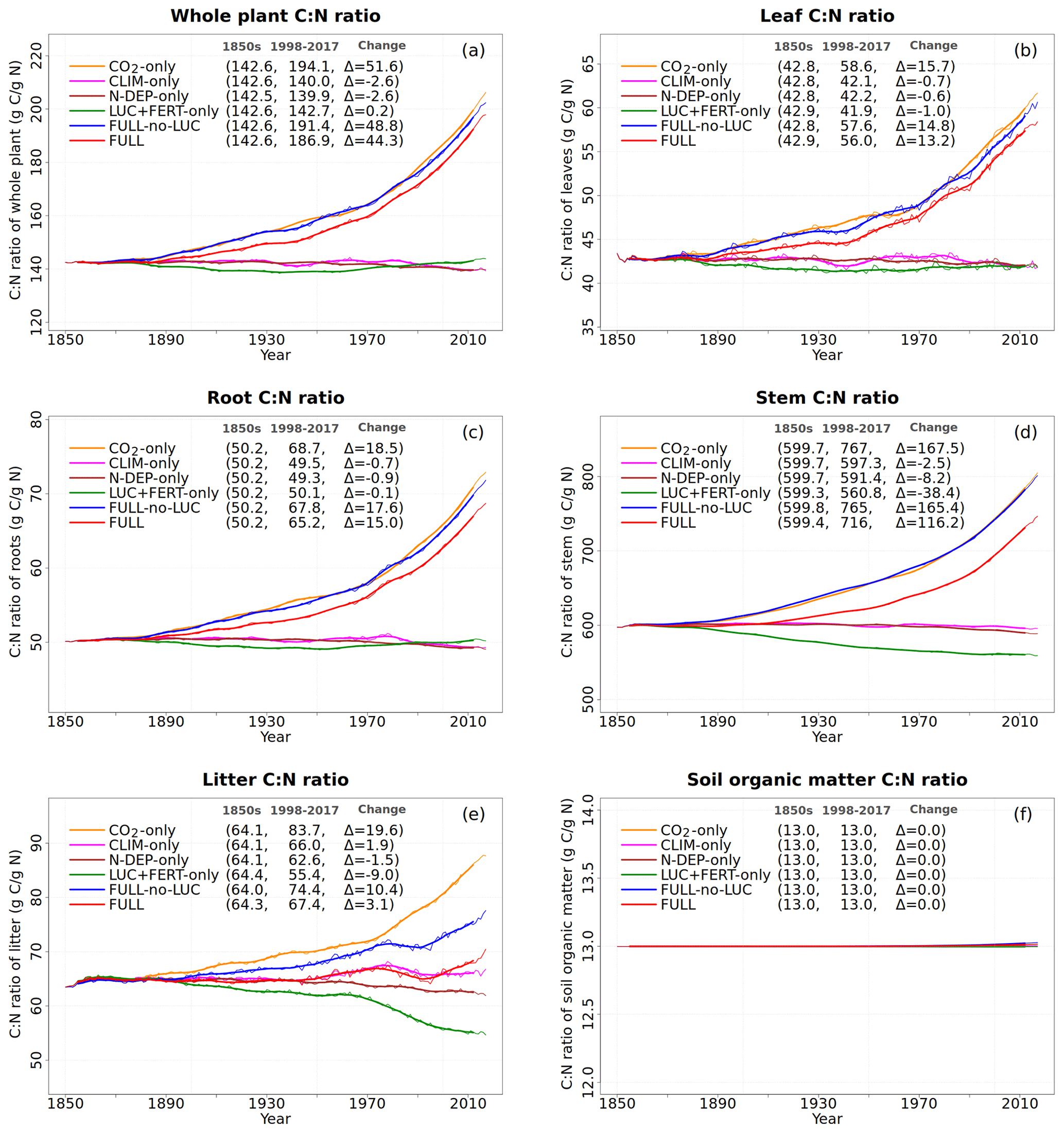
Figure 7Global annual values of C:N ratios for whole plant (a), leaves (b), root (c), stem (d), litter (e), and soil organic matter (f) pools from the primary six simulations. The values in the parentheses for legend entries show the average for the 1850s, the average for the 1998–2017 period, and the change between them. The thin lines show the annual values, and the thick lines show their 10-year moving average.

Figure 8Global annual values of net mineralization (a), nitrification (b), leaching (c), NH3 volatilization (d), and gaseous losses associated with nitrification (e) and denitrification (f) from the primary six simulations. The values in the parentheses for legend entries show the average for the 1850s, the average for the 1998–2017 period, and the change between them. The thin lines show the annual values, and the thick lines show their 10-year moving average.
Figure 8 shows the net mineralization flux (the net transfer of mineralized N from litter and humus pools to the mineral N pools as a result of the decomposition of organic matter), nitrification (N flux from to the pool), and the gaseous and leaching losses from the mineral pools. The net mineralization flux reduces in the CO2-only simulation (Fig. 8a, orange line) as N becomes locked up in the soil organic matter. A reduction in the pool size in response to increasing CO2 also yields a reduction in the nitrification flux over the historical period (Fig. 8b, orange line) since nitrification depends on the pool size (Eq. 19). Finally, leaching from the pool (Fig. 8c), NH3 volatilization (Fig. 8d), and the gaseous losses associated with nitrification from the pool (Fig. 8e) and denitrification from the pool (Fig. 8f) all reduce in response to a reduction in pool sizes of and in the CO2-only simulation.
5.2.2 Response to changing climate
The perturbation due to climate change alone over the historical period in the CLIM-only simulation (magenta-coloured lines in Figs. 4 to 8) is smaller than that due to increasing CO2. In Fig. 4a, changes in climate over the historical period increase GPP slightly by 3.60 Pg C yr−1 which in turn slightly increases vegetation (including leaf) C mass (Fig. 4b and c). The litter and soil carbon mass (Fig. 4d), however, decreases slightly due to increased decomposition rates associated with increasing temperature (see Fig. A2b). Both the increase in BNF due to increasing temperature (magenta line in Fig. 2a) and the reduction in litter and soil N mass (Fig. 5c) due to increasing decomposition and higher net N mineralization (Fig. 8a, magenta line) make more N available. This results in a slight increase in vegetation and leaf N mass (Fig. 5a and b) and the (Fig. 5e) pool which is the primary mineral pool in soils under vegetated regions. The global pool, in contrast, decreases in the CLIM-only simulation (Fig. 5f) with the reduction primarily occurring in arid regions where the amounts are very large (see Fig. 9 which shows the geographical distribution of the primary C and N pools). The geographical distribution of (Fig. 9a) generally follows the geographical distribution of BNF but with higher values in areas where cropland exists and where N deposition is high. The geographical distribution of (Fig. 9b) generally shows lower values than except in the desert regions where lack of denitrification leads to a large buildup of the pool (as explained earlier in Sect. 3.4.2). Although Fig. 9 shows the geographical distribution of mineral N pools from the FULL simulation, the geographical distribution of pools is broadly similar between different simulations with obvious differences such as lack of hot spots of N deposition and fertilizer input in simulations in which these forcings stay at their pre-industrial levels. Figure 9 also shows the simulated geographical distribution of C and N pools in the vegetation and soil organic matter. The increase in GPP due to changing climate increases the N demand (Fig. 6a, magenta line) but unlike the CO2-only simulation, the plant N uptake increases since the and pools increase in size over the vegetated area in response to increased mineralization (Fig. 8a, magenta line) and increased BNF (Fig. 3a, magenta line). The increase in plant N uptake comes from the increase in passive plant N uptake (Fig. 6c) while the active plant N uptake reduces (Fig. 6d). Active and passive plant N uptakes are inversely correlated. This is by design since active plant N uptake increases when passive plant N uptake reduces and vice versa, although eventually both depend on the size of available mineral N pools. Enhancement of plant N uptake due to changes in climate, despite increases in GPP associated with a small increase in Vcmax (Fig. 5d), leads to a small reduction in the C:N ratio of all plant tissues (Fig. 7). The litter C:N, in contrast, shows a small increase since not all N makes its way to the litter, as a specified fraction of 0.54 (Table A1) leaf N is resorbed from deciduous trees leaves prior to leaf fall (Fig. 7e). Although the leaf C:N ratio decreases in the CLIM-only simulation, in response to increased BNF and increased mineralization, this decrease is not large enough to overcome the effect of resorption, and as a result the C:N litter increases.
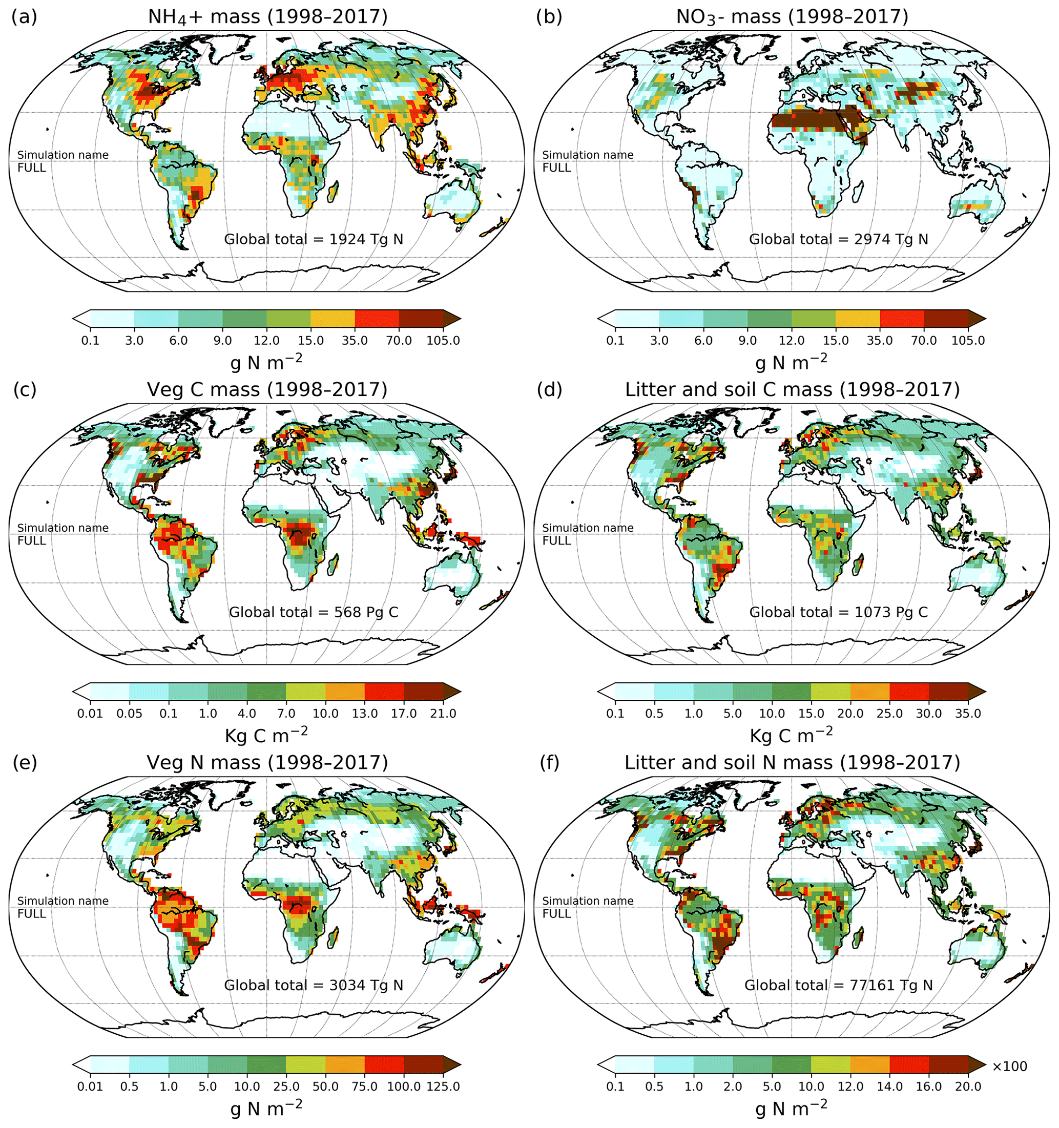
Figure 9Geographical distribution of primary C and N pools. Ammonium (a), nitrate (b), vegetation C mass (c), litter and soil C mass (d), vegetation N mass (e), and litter and soil N mass (f). The global total values shown are averaged over the 1998–2017 period.
Finally, the small increase in pool sizes of and leads to a small increase in leaching, volatilization, and gaseous losses associated with nitrification and denitrification (Fig. 8).
5.2.3 Response to N deposition
The simulated response of GPP to changes in N deposition (brown line) over the historical period is smaller than that for CO2 and climate (Fig. 4a). The small increase in GPP of 2.0 Pg C yr−1 leads to commensurately small increases in vegetation (Fig. 4b) and litter plus soil (Fig. 4d) C mass. Vegetation and leaf N mass (Fig. 5a and b) also increase in response to N deposition and so do mineral pools of and (Fig. 5e and f). The increase in GPP in the simulation with N deposition results from an increase in Vcmax rates (Fig. 5d) associated with an increase in leaf N amount (Fig. 5b). N demand increases marginally, and so does plant N uptake in response to N deposition (Fig. 6). As would be intuitively expected, the C:N ratio of the whole plant; its components of leaves, stem, and root; and litter decreases slightly in response to N deposition (Fig. 7). Net N mineralization, nitrification, leaching, volatilization, and gaseous losses associated with nitrification and denitrification all increase in response to N deposition (Fig. 8).
5.2.4 Response to LUC and fertilizer input
The simulated response to LUC, which reflects an increase in crop area and increased fertilizer deposition rates, over the historical period is shown by dark-green lines in Figs. 4 to 8. The increase in fertilizer input is a much bigger perturbation to the N cycle system than N deposition. Figure 2 shows that at the global scale the fertilizer inputs increase from 0 to ∼92 Tg N yr−1 over the historical period, while the combined and N deposition rate increases from around 20 to 65 Tg N yr−1. In addition, because of higher-per-unit-area BNF rates over crop areas than over natural vegetation, the increase in the crop area in this simulation leads to an increase in anthropogenic BNF from about 20 to 56 Tg N yr−1 over the historical period. All together increasing the crop area and fertilizer inputs implies an additional ∼130 Tg N yr−1 being input into the terrestrial N cycle in the present day compared to the pre-industrial period, contrasting an increase of only 45 Tg N yr−1 for the N deposition forcing.
The global increase in fertilizer input over the historical period leads to higher and pools (Fig. 5e and f). Although both fertilizer and BNF contribute to the pool, the pool also increases through the nitrification flux (Fig. 8b). An increase in crop area over the historical period results in deforestation of natural vegetation that reduces vegetation biomass (Fig. 4b). However, soil carbon mass also decreases (Fig. 4d) despite higher litter inputs. This is because a higher soil decomposition rate over cropland areas is assumed to simulate soil carbon loss due to tillage and other agricultural practices. This is consistent with empirical measurements of soil carbon loss over deforested areas which are converted to croplands (Wei et al., 2014). Fertilizer application only occurs over crop areas which increases the Vcmax rates for crops, and, as expected, this yields an increase in globally averaged Vcmax (Fig. 5d). A corresponding large increase in leaf N amount (Fig. 5b) is, however, not seen because vegetation (and therefore leaf) N (Fig. 5a and b) is also lost through deforestation. In addition, Vcmax is essentially a flux (expressed per unit leaf area) that is averaged over the whole year, while leaf and vegetation N pools are sampled at the end of each year and all crops in the Northern Hemisphere above 30∘ N are harvested before the year end. Vegetation N mass, in fact, decreases in conjunction with vegetation C mass (Fig. 4b). Plant N demand reduces (Fig. 6a) and plant N uptake increases (Fig. 6b), driven by crop PFTs in response to fertilizer input, as would be intuitively expected. The increase in plant N uptake comes from the increase in passive N uptake, in response to increases in pool sizes of and over crop areas, while active plant N uptake decreases since passive uptake can more than keep up with the demand over cropland areas. While the C:N ratio of vegetation biomass decreases over cropland areas in response to fertilizer input (not shown), this is not seen in the globally averaged C:N ratio of vegetation (Fig. 7a) and its components because C and N are also lost through deforestation and the fact that crop biomass is harvested. The C:N ratio of the global litter pool, however, decreases in response to litter from crops which becomes rich in N as fertilizer application rates increase. Finally, in Fig. 8, global net N mineralization, nitrification, leaching, volatilization, and gaseous losses associated with nitrification and denitrification all increase by a large amount in response to an increase in fertilizer input.
5.2.5 Response to all forcings
We can now evaluate and understand the simulated response of the FULL simulation to all forcings (red line in Figs. 4–8). The increase in GPP in the FULL simulation (14.5 Pg C yr−1) in Fig. 4a over the historical period is driven by a GPP increase associated with an increase in CO2 (7.5 Pg C yr−1), changing climate (3.6 Pg C yr−1), and N deposition (2.0 Pg C yr−1). The increases associated with these individual forcings add up to 13.1 Pg C yr−1, indicating that synergistic effects between forcings contribute to the additional 1.4 Pg C yr−1 increase in GPP. The changes in vegetation and soil plus litter carbon mass (Fig. 4b and d) in the FULL simulation are similarly driven by these three factors, but, in addition, LUC contributes to decreases in vegetation and soil carbon mass as natural vegetation is deforested to accommodate for increases in the crop area. Vegetation and leaf N mass (Fig. 5a and b) decrease in the FULL simulation, driven primarily by the response to increasing CO2 (orange line compared to the red line), while changes in litter and soil N mass are affected variably by all forcings (Fig. 5c). Changes in Vcmax (Fig. 5d) are similarly affected by all forcings: increasing CO2 leads to a decrease in globally averaged Vcmax values while changes in climate, N deposition, and fertilizer inputs lead to increases in Vcmax values with the net result being a small decrease over the historical period. The increase in global mass in the FULL simulation is driven primarily by the increase in fertilizer input (Fig. 5e, red versus green line). The changes in mass, in contrast, are primarily the result of changes in climate (Fig. 5f, magenta line) which causes a decrease in mass from about 1940 to 1970 and changes in N deposition and fertilizer input (Fig. 5f, green and brown lines) which contribute to the increase in mass later on in the historical period. The increase in N demand (Fig. 6a) over the historical period is also driven primarily by the increase in atmospheric CO2. Plant N uptake (Fig. 6b) decreases in response to increasing CO2 but increases in response to changes in climate, N deposition, and fertilizer inputs such that the net change over the historical period is a small decrease. The increase in the C:N ratio of vegetation and its components (leaves, stem, and root) is driven primarily by an increase in atmospheric CO2 (Fig. 7a, red versus orange line). Litter C:N in the FULL simulation, in contrast, does not change substantially over the historical period in a globally averaged sense as the increase in the C:N ratio of litter associated with an increase in atmospheric CO2 is mostly compensated for by the decrease associated with an increase in N deposition and fertilizer application. The simulated change in global net N mineralization (Fig. 8a) in the FULL simulation, over the historical period, is small since the decrease in net N mineralization due to increasing CO2 (orange line) is compensated for by the increase caused by changes in climate, N deposition, and fertilizer inputs (magenta, brown, and green lines, respectively). The remaining fluxes of nitrification, leaching, NH3 volatilization, and gaseous losses associated with nitrification and denitrification in the FULL simulation (Fig. 8) are all strongly influenced by fertilizer input (green line compared to red line).
Table 2 compares simulated values of all primary N pools and fluxes from the FULL simulation with other modelling and quasi observation-based studies. Simulated values are averaged over the 1998–2017 period. Where available, time periods for other modelling and quasi observation-based studies to which estimates correspond are also noted. For the most part simulated pools and fluxes lie within the range of existing studies with the exception of N2 and NO emissions which are somewhat higher.
5.2.6 Response to all forcings except LUC
The FULL-no-LUC simulation includes all forcings except LUC (blue line in Figs. 4–8) and corroborates several of the points mentioned above. In this simulation the crop area stays at its 1850 value. Figure 2b (blue line) shows increasing global fertilizer input in this simulation despite the crop area staying at its 1850 value since fertilizer application rates per unit area increase over the historical period. In the absence of the LUC, vegetation C mass (Fig. 4b) and soil plus litter C (Fig. 4d) and N (Fig. 5c) are higher in the FULL-no-LUC simulation compared to in the FULL simulation. N demand (Fig. 6a) is slightly higher in FULL-no LUC than in the FULL simulation because there is more standing vegetation biomass that is responding to increasing CO2. The increase in volatilization, leaching, and gaseous losses associated with nitrification and denitrification (Fig. 8c–f) are all primarily caused by increased fertilizer input over the specified 1850 crop area. The increase in N losses associated with these processes, over the historical period, is much lower in the FULL-no-LUC simulation than in the FULL simulation since the crop area stays at its 1850 values.
5.3 Comparison of FULL and ORIGINAL simulations
We now compare the results from the FULL simulation that includes the N cycle with that from the ORIGINAL simulation that does not include the N cycle. Both simulations are driven with all forcings over the historical period. Figure 4a shows that the global GPP values in the FULL (red line) and ORIGINAL (purple line) simulations are quite similar although the rate of increase in GPP in the FULL simulation is slightly higher than in the ORIGINAL simulation. As a result, simulated global vegetation biomass is somewhat higher in the FULL simulation (Fig. 4b). The simulated global litter and soil carbon mass (Fig. 4d) is, however, lower in the FULL simulation (1073 Pg C) compared to the ORIGINAL simulation (1142 Pg C), and this decrease mainly comes from a decrease at higher latitudes (not shown) due to a decrease in GPP (Fig. 10a). The lower GPP in the FULL simulation, combined with the slow decomposition at cold high latitudes, results in a lower equilibrium for litter and soil carbon compared with the ORIGINAL simulation. Litter mass contributes about 80 Pg C to the total dead carbon mass. Overall both estimates of 1073 and 1142 Pg C are somewhat lower than the bulk-density-corrected estimate of 1230 Pg C based on the Harmonized World Soil Database (HWSD) v.1.2 (Köchy et al., 2015). One reason for this is that CLASSIC does not yet represent permafrost-related soil C processes.
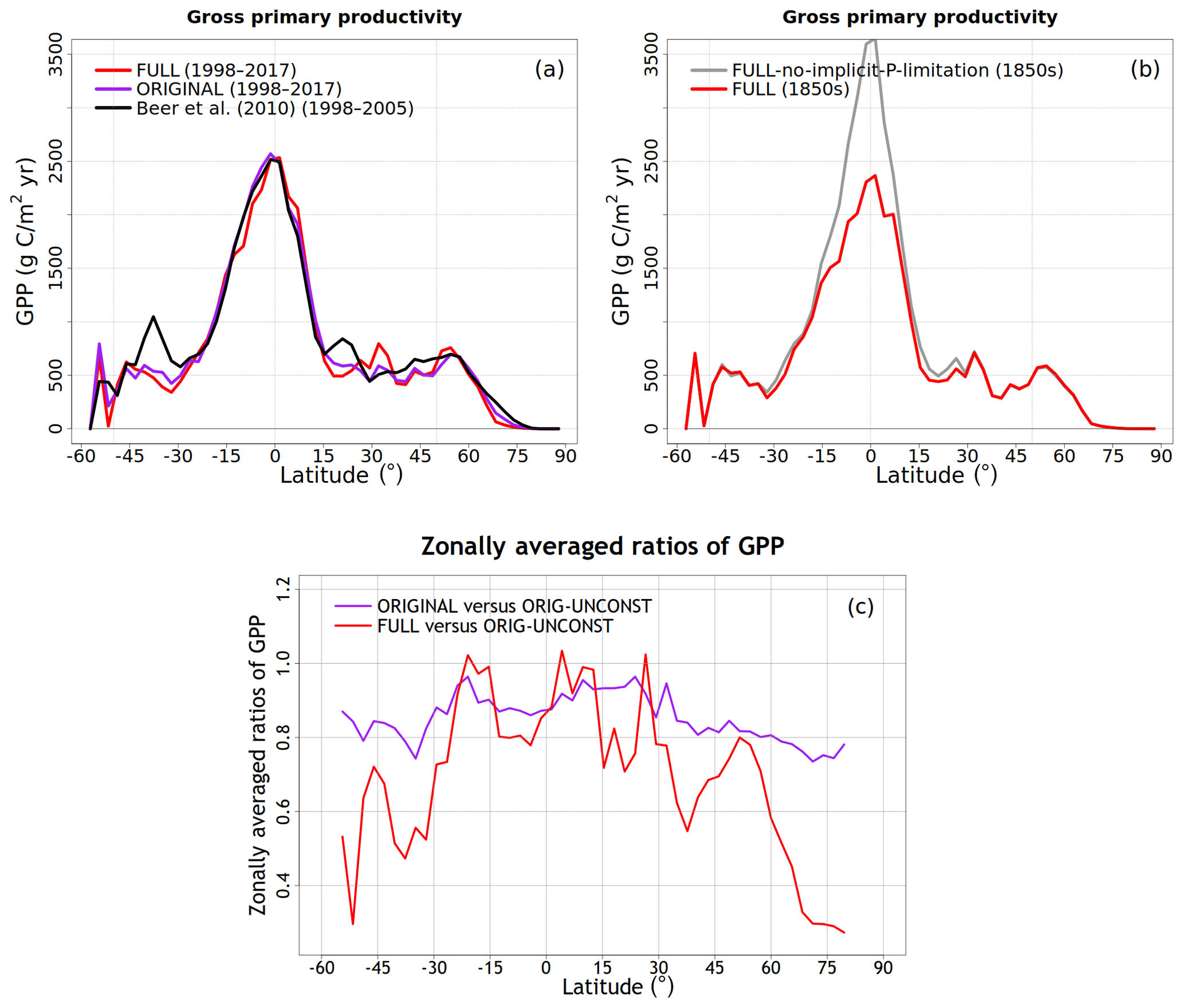
Figure 10Comparison of zonal distribution of gross primary productivity (GPP) and the effect of GPP downregulation compared to the ORIG-UNCONST simulation. (a) Compares zonal distribution of GPP from FULL and ORIGINAL simulations with observation-based estimate from Beer at al. (2010) for the present day. (b) Compares the zonal distribution of GPP from the pre-industrial simulation, corresponding to 1850 conditions, from the FULL and FULL-no-implicit-P-limitation simulations to illustrate the effect of not reducing the Γ1 parameter for calculating Vcmax for the broadleaf-evergreen-tree PFT that implicitly accounts for phosphorus limitation. (c) Shows the zonally averaged ratios of GPP from the ORIGINAL and FULL simulations versus those from the ORIG-UNCONST simulations to illustrate how downregulation acts in the ORIGINAL and FULL simulations.
Figure 10a shows that the zonal distribution of GPP from the FULL and ORIGINAL simulations, for the 1998–2017 period, compares reasonably well to the observation-based estimate from Beer et al. (2010). The FULL simulation has slightly lower productivity at high latitudes than the ORIGINAL simulation, as mentioned above. Overall, however, the inclusion of the N cycle does not change the zonal distribution of GPP in the model substantially, which is determined primarily by the geographical distribution of climate. Figure 10b compares the zonal distribution of GPP from the pre-industrial simulation (corresponding to the 1850s) from the FULL and FULL-with-no-implicit-P-limitation simulations to illustrate the high GPP in the tropics where P limitation and not N limitation affects GPP and is the reason for choosing a lower value of Γ1 in Eq. (31) for the broadleaf evergreen tree PFT.
The global GPP in the ORIGINAL and FULL simulations averaged over the period 1998–2017 (120.0 and 120.4 Pg C yr−1, respectively) are around 15 % lower compared to that in the ORIG-UNCONST simulation (142 Pg C yr−1), as shown in Fig. 4a, yielding a global downregulation factor of about 0.85. Figure 10c shows how downregulation works in the ORIGINAL and FULL simulations in a zonally averaged sense. Ratios of annual GPP averaged over the 1998–2017 period from the ORIGINAL versus ORIG-UNCONST simulations and from the FULL versus ORIG-UNCONST simulations were first calculated for each grid cell and then zonally averaged over the land grid cells. Ratios can be misleading, especially for grid cells with low values, for example, in the desert regions. In addition, these ratios also depend on the specified Vcmax values in the ORIG-UNCONST simulation. In Fig. 10c, the purple line for the ORIGINAL simulation exhibits values of around 0.8, consistent with the global downregulation of around 0.85 and the fact that the same scalar downregulation multiplier is used everywhere on the globe (Eq. 1). The red line for the FULL simulation, however, indicates a pattern of higher downregulation at high latitudes. The peaks in the red line, especially the one around 23∘ N (Sahara), are due to higher values in selected grid cells in dry and arid regions where the buildup of in the soil (due to reduced denitrification) increases Vcmax and thus GPP in the run with the N cycle, leading to higher ratios although the absolute GPP values still remain low.
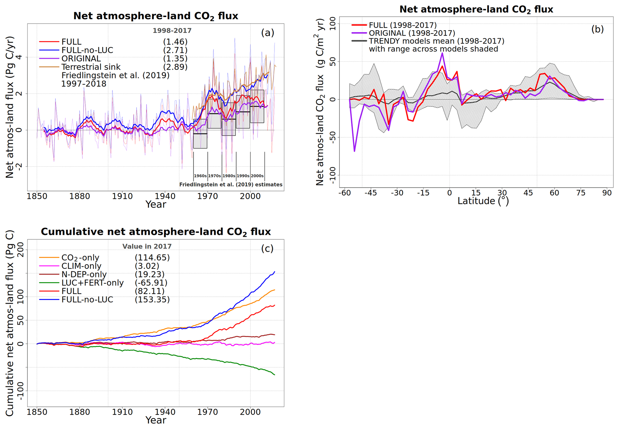
Figure 11Comparison of simulated net atmosphere–land CO2 flux from various simulations. (a) Compares globally summed values of net atmosphere–land CO2 flux from FULL, FULL-no-LUC simulation, and ORIGINAL simulations with estimate of terrestrial sink (dark-yellow line) and net atmosphere–land CO2 flux (grey bars) from Friedlingstein et al. (2019). The thin lines show the annual values, and the thick lines show their 10-year moving average. (b) Compares zonal distribution of net atmosphere–land CO2 flux from FULL and ORIGINAL simulations with the range from TRENDY models that contributed to the Friedlingstein et al. (2019) study. (c) Shows cumulative values of net atmosphere–land CO2 flux from the six primary simulations to investigate the contribution of each forcing to the cumulative land carbon sink over the historical period.
Figure 11a compares globally summed net atmosphere–land CO2 flux from the FULL, FULL-no-LUC, and ORIGINAL simulations with quasi observation-based estimates from the 2019 Global Carbon Project (Friedlingstein et al., 2019). There are two kinds of estimates in Fig. 11a from Friedlingstein et al. (2019): the first is the net atmosphere–land CO2 flux for the decades spanning the 1960s to the 2000s, which are shown as rectangular boxes with their corresponding mean values and ranges, and the second is the terrestrial sink from 1959–2018 (dark-yellow line). Positive values indicate a sink of carbon over land, and negative values indicate a source. The difference between the net atmosphere–land CO2 flux and the terrestrial sink is that the terrestrial sink minus the LUC emissions yields the net atmosphere–land CO2 flux. The atmosphere–land CO2 flux from the FULL-no-LUC simulation (blue line) is directly comparable to the terrestrial sink since 1959, since the FULL-no-LUC simulation includes no LUC, and shows that the simulated terrestrial sink compares fairly well to the estimates from Friedlingstein et al. (2019). Averaged over the period 1959–2017, the modelled and Global Carbon Project values are 2.0 and 2.1 Pg C yr−1, respectively. The net atmosphere–land CO2 flux from the FULL simulation mostly lies within the uncertainty range for the 5 decades considered, although it is on the higher side compared to estimates from Friedlingstein et al. (2019). The reason for this is that LUC emissions in CLASSIC are much lower than observation-based estimates, as discussed below in the context of Fig. 11c. CLASSIC simulates LUC emissions only in response to changes in the crop area, although changes in pasture area and wood harvesting also contribute to LUC emissions. The net atmosphere–land CO2 flux from the ORIGINAL simulation compares better than the FULL simulation with the estimates from Friedlingstein et al. (2019), because the photosynthesis downregulation parameter in the ORIGINAL simulation has been adjusted despite discrepancies in simulated LUC processes.
Figure 11b compares the zonal distribution of simulated net atmosphere–land CO2 flux from the FULL and ORIGINAL simulations with the model mean and range from the terrestrial ecosystem models that participated in the 2019 TRENDY model intercomparison and contributed results to the 2019 Global Carbon Project (Friedlingstein et al., 2019). The carbon sink simulated by CLASSIC in the Northern Hemisphere is broadly comparable to the model-mean estimate from the TRENDY models. However, in the tropics CLASSIC simulates a much stronger sink than the model mean, likely because of its lower LUC emissions.
5.4 Contribution of forcings to land C sink and sources
Figure 11c shows cumulative net atmosphere–land CO2 flux for the 1850–2017 period from the six primary simulations with the N cycle. These simulations facilitate the attribution of carbon uptake and release over the historical period to various forcings. The cumulative terrestrial sink in the FULL-no-LUC simulation for the period 1850–2017 is simulated to be ∼153 Pg C, and this compares reasonably well with the estimate of 185±50 Pg C for the period 1850–2014 from Le Quéré et al. (2018). An increase in CO2 (∼115 Pg C), change in climate (∼3 Pg C), and N deposition (∼19 Pg C) all contribute to this terrestrial sink. These three contributions add up to 137 Pg C, so the additional 16 Pg C is contributed by the synergistic effects between the three forcings. Quantified in this way, the contribution of increasing CO2 (115 out of 137 Pg C), climate change (3 out of 137 Pg C), and N deposition (19 out of 137 Pg C) to carbon uptake by land over the historical period (1850–2017) is calculated to be 84 %, 2 %, and 14 %, respectively. Cumulative LUC emissions simulated for the period 1850–2017 by CLASSIC can be estimated using negative cumulative net atmosphere–land CO2 flux of ∼66 Pg C from the LUC + FERT-only simulation. Alternatively, simulated LUC emissions can be calculated by taking the difference between cumulative net atmosphere–land CO2 flux from the FULL-no-LUC and FULL simulations (∼71 Pg C). While LUC emissions are highly uncertain, both of these estimates are much lower than the 195±75 Pg C estimate from Le Quéré et al. (2018).
The interactions between the terrestrial C and N cycles are complex, and our understanding of these interactions and their representation in models is based on empirical observations of various terrestrial ecosystem processes. In this paper, we have evaluated the response of these interactions by perturbing the coupled C and N cycle processes in the CLASSIC model with one forcing at a time over the historical period: (1) increase in CO2, (2) change in climate, (3) increase in N deposition, and (4) LUC with increasing fertilizer input. These simulations are easier to interpret, and the model response can be evaluated against both our conceptual knowledge and empirical observation-based data. Our assumption is that, if the model response to individual forcings is realistic and consistent with expectations based on empirical observations, then the response of the model to all forcings combined will also be realistic and easier to interpret, although we do expect and see synergistic effects between forcings.
The simulated response of coupled C and N cycles in CLASSIC to increasing atmospheric CO2 is an increase in the C:N ratio of vegetation components due to not only an increase in their C content but also a decrease in their N content. This model response is conceptually consistent with a meta-analysis of 75 field experiments of elevated CO2 as reported in Cotrufo et al. (1998), who find an average reduction in tissue N concentration of 14 %. Most studies analyzed in the Cotrufo et al. (1998) meta-analysis used ambient CO2 of around 350 ppm and elevated CO2 of around 650–700 ppm. In comparison, the plant N concentration in CLASSIC reduces by ∼26 % in response to a gradual increase in atmospheric CO2 from 285 to 407 ppm (an increase of 122 ppm) over the 1850–2017 period (whole plant C:N ratio increases from 142.6 to 194.1 in the CO2-only simulation, Fig. 7a). These two estimates cannot be compared directly – a majority (59 %) of Free-Air Carbon dioxide Enrichment (FACE) experiments last less than 3 years (Jones et al., 2014) and the vegetation experiences a large CO2 change of around 300–350 ppm, while the duration of our historical simulation is 167 years and the gradual increase in CO2 of 122 ppm over the historical period is much smaller.
The response of our model to a CO2 increase over the historical period is also consistent with the meta-analysis of McGuire et al. (1995), who report an average decrease in leaf N concentration of 21 % in response to elevated CO2 based on 77 studies, which is the primary reason for the downregulation of photosynthetic capacity. The simulated decrease in leaf N concentration in our study for the CO2-only experiment is around 27 % (leaf C:N ratio increases from 42.8 to 58.6 in the CO2-only simulation, Fig. 7b). However, the same caveats that apply to the comparison with the Cotrufo et al. (1998) study also apply to this comparison. The decrease in whole plant and leaf N concentrations in our results is conceptually consistent with the meta-analyses of McGuire et al. (1995) and Cotrufo et al. (1998). The decrease in whole plant N concentration in our CO2-only and FULL simulations is the result of both an increase in tissue C amount and a decrease in N amount. The decrease in tissue N amount is, in fact, necessary in our modelling framework to induce the required downregulation of photosynthesis to simulate the land carbon sink realistically over the historical period.
The meta-analysis of Liang et al. (2016) reports an increase in above- and belowground plant N pools in response to elevated CO2 associated with an increase in BNF, but since their results are based on pool sizes they cannot be compared directly to the N-concentration-based results from McGuire et al. (1995) and Cotrufo et al. (1998). Liang et al. (2016) also report results from short-term (≤3 years) and long-term (between 3 and 15 years) studies separately (their Fig. 3). They show that the increase in total plant and litter N pools becomes smaller for long-term studies. Regardless, the difference in timescales of empirical studies and the real world is a caveat that will always make it difficult to evaluate model results over long timescales.
The response of C and N cycles to changes in climate in our model (in the CLIM-only simulation) is also conceptually realistic. Globally, GPP increases in response to climate that gradually becomes warmer and wetter (see Fig. A2), and as a result vegetation biomass increases. Soil carbon mass, however, decreases (despite an increase in NPP inputs) since warmer temperatures also increase heterotrophic respiration (not shown). As a result of increased decomposition of soil organic matter, net N mineralization increases, and together with increased BNF the overall C:N ratio of vegetation and leaves decreases, which leads to a Vcmax increase. The small increase in Vcmax, due to increased mineralization, thus also contributes to an increase in GPP over and above that due to a change in climate alone and therefore compensates for the amount of carbon lost due to increased soil organic matter decomposition associated with warmer temperatures. This behaviour is consistent with land C cycle models showing a reduction in the absolute value of the strength of the carbon–climate feedback when they include coupling of C and N cycles (Arora et al., 2020).
The modelled differences in PFT-specific values of Vcmax, in our framework, come through differences in simulated values of leaf N amount (NL) that depend on not only BNF (given that BNF is the primary natural source of N input into the coupled soil–vegetation system) but also differences in mineralization that are governed by climate. NL values, however, also depend on leaf phenology, allocation of carbon and nitrogen, turnover rates, transpiration (which brings in N through passive uptake), and almost every aspect of plant biogeochemistry which affects a PFT's net primary productivity and therefore N demand. Modelled increases in GPP in response to N deposition come through an increase in leaf N amount and therefore Vcmax values.
Finally, changes in land use associated with an increase in crop area and the associated increase in fertilizer application rates lead to the largest increase in leaching, NH3 volatilization, and gaseous losses associated with nitrification and denitrification among all forcings. Overall, the model response to perturbation by all individual forcings is realistic, conceptually expected, and of the right sign (positive or negative) although it is difficult to evaluate the magnitude of these responses in the absence of directly comparable observation-based estimates.
Despite the model responses to individual forcings that appear consistent with our conceptual understanding of coupled C and N cycles, our modelling framework misses an important feedback process that has been observed in FACE and other experiments related to changes in natural BNF. FACE sites and other empirical studies report an increase in natural BNF rates at elevated CO2 (McGuire et al., 1995; Liang et al., 2016) and a decrease in natural BNF rates when additional N is applied to soils (Salvagiotti et al., 2008; Ochoa-Hueso et al., 2013). On a broad scale this is intuitively expected, but the biological processes behind changes in BNF rates remain largely unclear. A response can still be parameterized even if the underlying physical and biological processes are not well understood. For instance, Goll et al. (2012) parameterize BNF as an increasing and saturating function of NPP: . This approach, however, does not account for the driver behind the increase in NPP – increasing atmospheric CO2, change in environmental conditions (e.g., wetter and warmer conditions), or increased N deposition. Clearly, increasing BNF if the NPP increase is due to N deposition is inconsistent with empirical observations. Over the historical period an increase in atmospheric CO2 has been associated with an increase in N deposition, so to some extent changes in BNF due to both forcings will cancel each other out. We realize the importance of changes in BNF, given it is the single largest natural flux of N into the coupled soil–vegetation system, yet it is highly uncertain, and we aim to address these issues in a future version of the model by exploring existing BNF formulations. Meyerholt et al. (2016), for example, demonstrate the uncertainty arising from the use of five different BNF parameterizations in the context of the O-CN model. They use formulations that parameterize BNF as a function of (1) evapotranspiration; (2) NPP; (3) the leaf C:N ratio, which takes into account the energy cost for N fixation (Fisher et al., 2010); (4) plant N demand; and (5) an optimality-based approach that follows Rastetter et al. (2001) in which BNF only occurs when the carbon cost of N fixation is lower than the carbon cost of root N uptake. The approach used in our study is closest to the one that is based on evapotranspiration but makes the distinction in BNF rates over natural and agricultural areas.
The reduction in photosynthesis rates in response to N limitation is the most important linkage between C and N cycles, and yet it too is parameterized differently across models. Given that leaf N amount and photosynthetic capacity are strongly correlated (Evans, 1989; Field and Mooney, 1986; Garnier et al., 1999), photosynthesis downregulation due to N limitation reduces photosynthetic capacity and thus the GPP flux. Yet models reduce both NPP (Wiltshire et al., 2020) and Vcmax rates and thus GPP, (Zaehle and Friend, 2010; Wania et al., 2012; von Bloh et al., 2018) in response to N limitation. Vcmax rates may themselves be parameterized as a function of the leaf N amount directly (von Bloh et al., 2018; Zaehle and Friend, 2010) or the leaf C:N ratio (Wania et al., 2012). In this study, we have parameterized Vcmax rates as a function of the leaf N amount (Eq. 31) since the use of the leaf C:N ratio leads to an incorrect seasonal variation in Vcmax. If an increase in the leaf C:N ratio, as a result of an increase in atmospheric CO2, leads to a decrease in Vcmax rates over the historical period, then it implies that Vcmax is inversely related to leaf C:N ratios. Since leaf C:N ratios peak during the growing season (Li et al., 2017) this also implies Vcmax rates are lower during the peak growing season than at its start, and this is in contrast to observations that show an increase in Vcmax during the growing season (e.g., see Fig. 1a of Bauerle et al., 2012).
Our framework assumes a constant C:N ratio of 13 for soil organic matter (C:NH), an assumption also made in other models (e.g., Wania et al., 2012; Zhang et al., 2018). This assumption is also broadly consistent with Zhao et al. (2019), who attempt to model C:N of soil organic matter, among other soil properties, as a function of mean annual temperature and precipitation using machine-learning algorithms (their Fig. 2h). It is difficult to currently establish if increasing atmospheric CO2 is changing C:NH, given the large heterogeneity in soil organic C and N densities and the difficulty in measuring small trends for such large global pools. A choice of a somewhat different value for all PFTs or had we chosen specified constant PFT-dependent values of C:NH is of relatively less importance in this context since the model is spun up to equilibrium for 1850 conditions anyway. It is the change in C:NH over time that is of importance. The assumption of constant C:NH is the key to yielding a decrease in vegetation N mass, and therefore leaf N mass and Vcmax, as CO2 increases, in our framework. Without a decrease in Vcmax in our modelling framework, in response to elevated CO2 we cannot achieve the downregulation noted by McGuire et al. (1995) in their meta-analysis and the simulated carbon sink over the historical period would be greater than observed as noted above. It is possible that we are simulating the reduction in leaf N mass, in response to elevated CO2, for a wrong reason, in which case our model processes need to be revisited based on additional empirical data. If our assumption of constant or extremely slowly changing C:NH is indeed severely unrealistic, this necessitates a point of caution about a realistic land carbon sink being simulated over the historical period with such an assumption.
Related to this assumption is also the fact that we cannot make decomposition rates of soil organic matter a function of its C:N ratio since this is assumed to be a constant. It is well known that after climate, litter and soil organic matter decomposition rates are controlled by their C:N ratio (Manzoni et al., 2008). Litter decomposition rates can still be made a function of the litter C:N ratio, and we aim to do this for a future model version.
The work presented in this study of coupling C and N cycles in CLASSIC yields a framework that we can build upon to make model processes more realistic, test the effect of various model assumptions, parameterize existing processes in other ways, include additional processes, and evaluate model responses at FLUXNET sites to constrain model parameters.
The rates of change in N in the and pools (in gN m−2), and , respectively, are given by
and all fluxes are represented in units of . is the rate of biological N fixation which solely contributes to the pool; is the fertilizer input which is assumed to contribute only to the pool, and and are atmospheric deposition rates that contribute to the and pools, respectively. Biological N fixation, fertilizer input, and atmospheric deposition are the three routes through which N enters the coupled soil–vegetation system. and are the mineralization flux from the litter and soil organic matter pools, respectively, associated with their decomposition. We assume mineralization of humus and litter pools only contributes to the pool. and indicate immobilization of N from the and pools, respectively, to the humus N pool which implies microbes (which are not represented explicitly) are part of the humus pool. Combined together the terms yield the net mineralization rate. is the rate of ammonia (NH3) volatilization, and is the leaching of N that occurs only from the pool. The positively charged ammonium ions are attracted to the negatively charged soil particles, and as a result it is primarily the negatively charged nitrate ions that leach through the soil (Porporato et al., 2003; Xu-Ri and Prentice, 2008). and are uptakes of and by plants, respectively. The nitrification flux from the to pool is represented by , which also results in the release of the nitrous oxide (N2O), a greenhouse gas, and nitric oxide (NO) through nitrifier denitrification represented by the terms and INO, respectively. Finally, , , and ENO are the gaseous losses of N2 (nitrogen gas), N2O, and NO from the pool associated with denitrification. N is thus lost through the soil–vegetation system via leaching in runoff and through gaseous losses of , INO, , , ENO, and .
The structural and non-structural N pools in roots are written as NR,S and NR,NS, respectively, and they are similarly denoted for stem (NS,S and NS,NS) and leaves (NL,S and NL,NS), and together the structural and non-structural pools make the total N pool in the leaf (), root (), and stem () components. The rate change equation for structural and non-structural N pools in roots are given by
Similarly to the uptake of carbon by leaves and its subsequent allocation to root and stem components, N is taken up by roots and then allocated to leaves and the stem. AR2L and AR2S represent the allocation of N from roots to leaves and the stem, respectively. The terms RL2R and RR2L represent the reallocation of N between the non-structural components of the root and leaves. RL2R is the N reallocated from leaves to the root representing resorption of a fraction of leaf N during leaf fall for deciduous-tree PFTs. RR2L indicates reallocation of N from roots to leaves (termed reallocation in Fig. 2) at the time of leaf-out for deciduous-tree PFTs. At times other than leaf-out and leaf fall and for other PFTs, these two terms are zero. TR,NS2S is the one-way transfer of N from the non-structural to the structural root pool, and similarly to the carbon pools, once N is converted to its structural form it cannot be converted back to its non-structural form. Finally, the litterfall due to the turnover of roots occurs from both the structural (LFR,S) and non-structural (LFR,NS) N pools.
The rate change equations for non-structural and structural components of leaves are written as
where TL,NS2S is the one way transfer of N from the non-structural leaf component to its structural N pool and RS2L indicates reallocation of N from the stem to leaves (similarly to RR2L) at the time of leaf-out for deciduous-tree PFTs. Litterfall occurs from both the structural (LFL,S) and non-structural (LFL,NS) N pools of leaves, and all other terms have been previously defined.
Finally, the rate change equations for non-structural and structural components of the stem are written as
where LFS,NS and LFS,S represent stem litter from the non-structural and structural components and TS,NS2S is the one-way transfer of N from the non-structural stem component to its structural N pool. All other terms have been previously defined.
Adding Eqs. (A3) to (A8) yields rate of change in N in the entire vegetation pool (NV) as
which indicates how the dynamically varying vegetation N pool is governed by mineral N uptake from the and pools and litterfall from the structural and non-structural components of the leaves, stem, and root pools. LFR is the total N litter generation from the root pool and the sum of litter generation from its structural and non-structural components (), and similar denotation is used for the leaves (LFL) and the stem (LFS) pools.
The rate change equations for the organic N pools in the litter (ND) and soil (NH) pools are written as follows:
where HN,D2H is the transfer of humidified organic matter from litter to the soil organic matter pool, and all other terms have been previously defined.
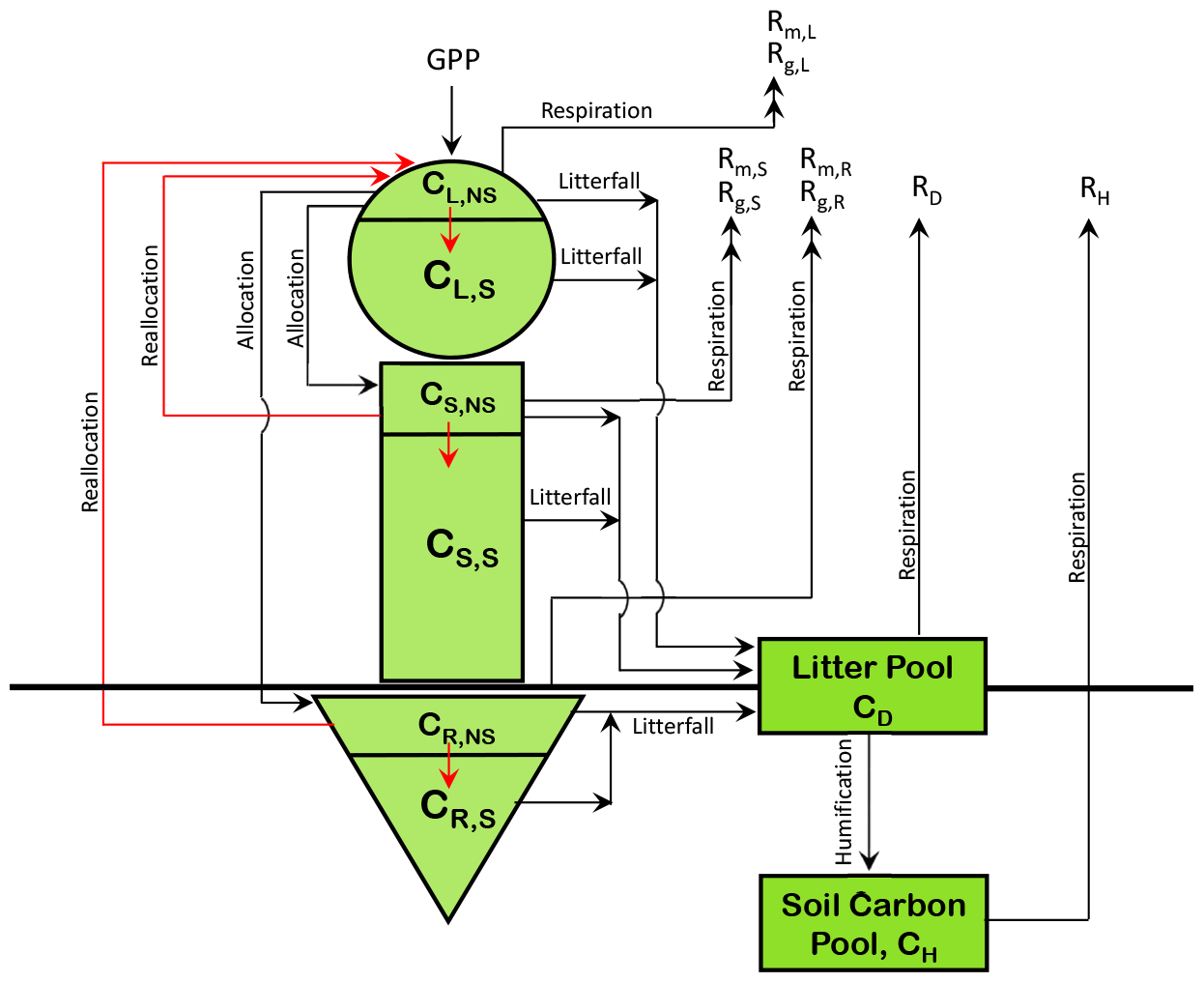
Figure A1The structure of the CLASSIC model used in this study, upon which the N cycle is implemented, with its carbon pools and fluxes. The fluxes of non-structural carbon are shown in a red colour.
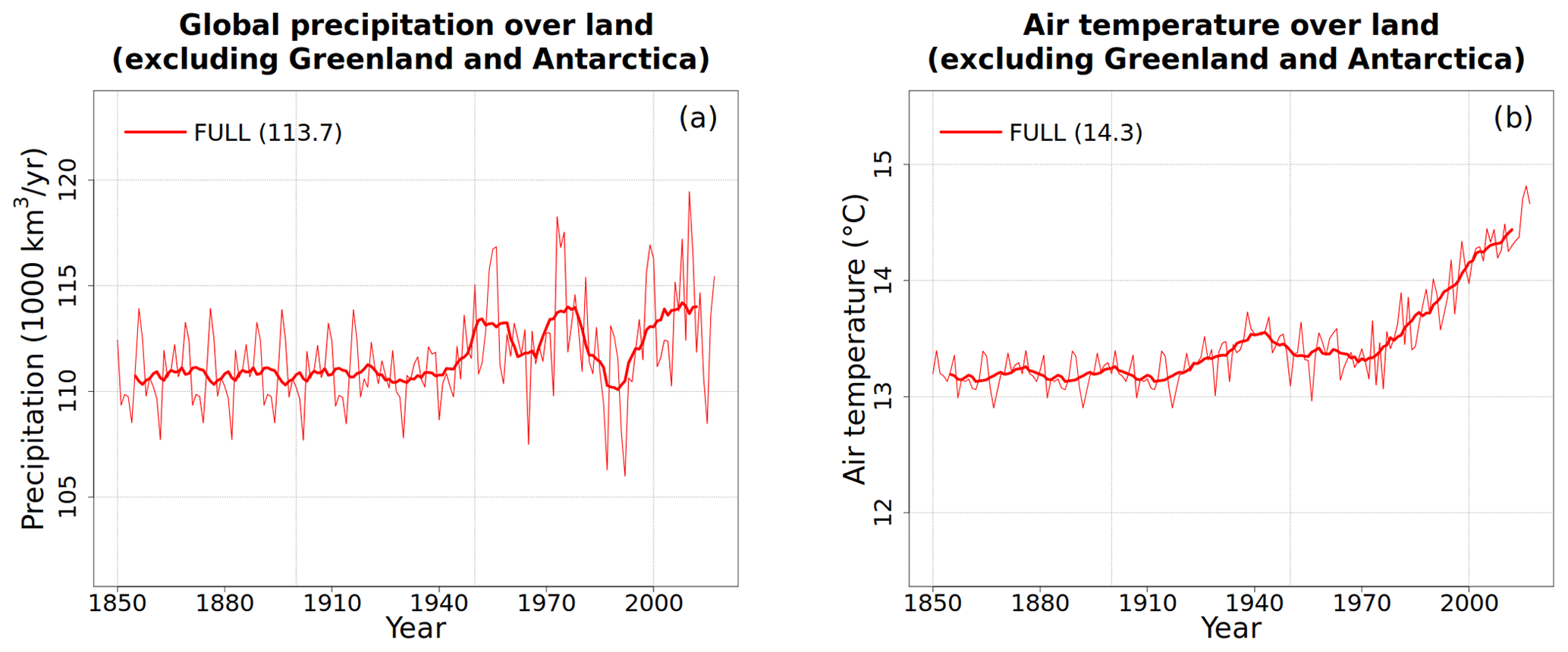
Figure A2Annual values of global precipitation (a) and air temperature (b) over land in the CRU-JRA reanalysis data that are used to drive the model. The data are available for the period 1901–2017. In the absence of meteorological data for the period 1851–1900, data from the period 1901–1925 are used twice. The thin lines are the annual values, and the thick line is their 10-year running mean. The values in the parentheses in the legend show average values over the last 20 years.
Table A1Model parameters for various model parameterizations. The corresponding equation in which the parameter appears in the main text is also noted. Model parameters may be scalar or an array (if they are PFT dependent) in which case they are written according to the following structure in the table below.
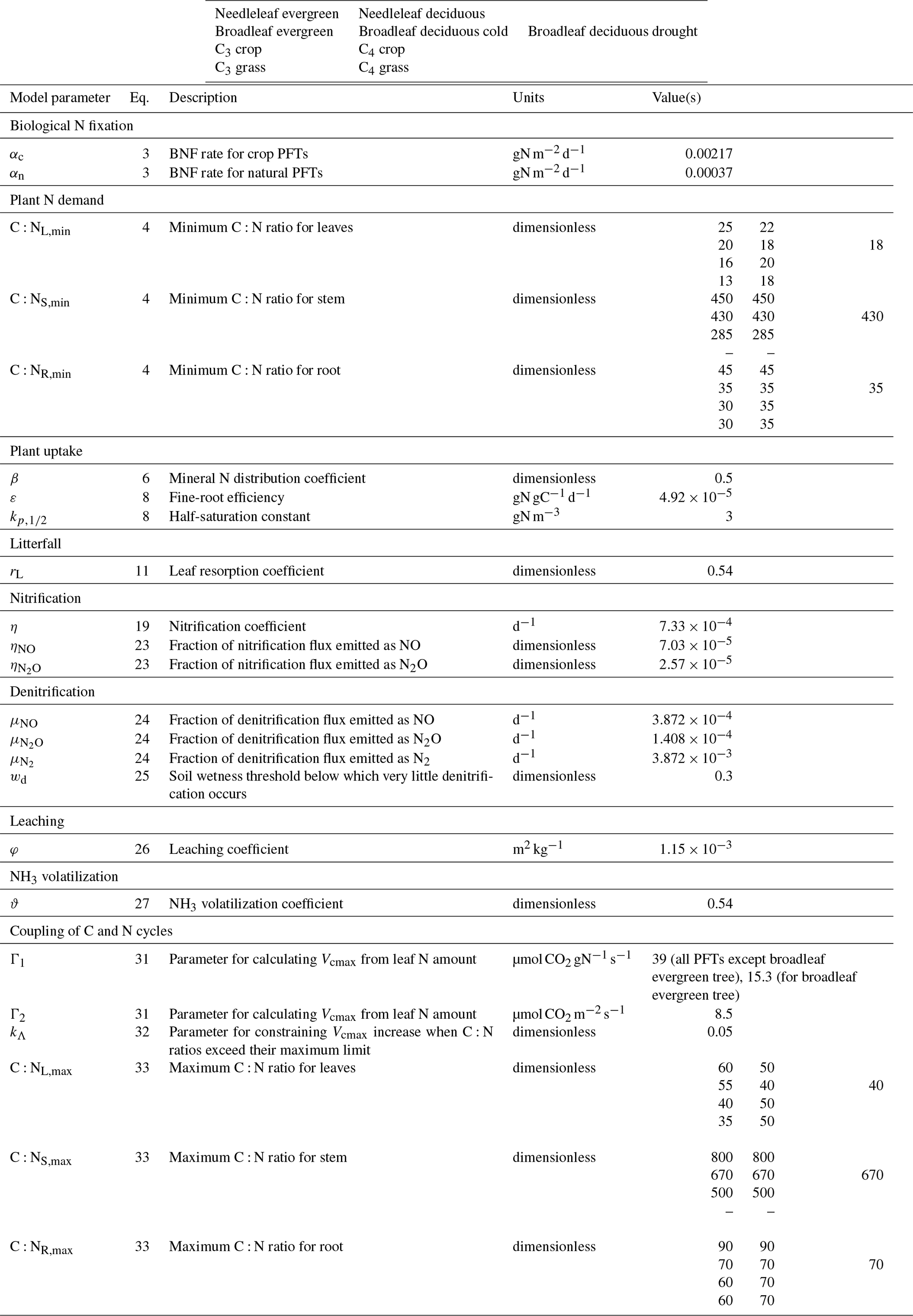
Model code used in this study can be obtained from https://doi.org/10.5281/zenodo.4455929 (Arora and Asaadi, 2021).
AA implemented the N cycle in the CLASSIC code, put together all the N-cycle-related input data, and performed all the simulations. VKA and AA wrote the manuscript.
The authors declare that they have no conflict of interest.
We are grateful to and thank Joe Melton and Paul Bartlett for their comments on an earlier version of this paper. We are grateful to Stefan Gerber and David Wårlind for their reviewer comments which greatly improved this paper. We also gratefully acknowledge Sönke Zaehle, the handling editor for this paper, for his time and effort.
This paper was edited by Sönke Zaehle and reviewed by Stefan Gerber and David Wårlind.
Alexandrov, G. and Oikawa, T.: TsuBiMo: a biosphere model of the CO2-fertilization effect, Clim. Res., 19, 265–270, 2002.
Aragão, L. E. O. C., Malhi, Y., Metcalfe, D. B., Silva-Espejo, J. E., Jiménez, E., Navarrete, D., Almeida, S., Costa, A. C. L., Salinas, N., Phillips, O. L., Anderson, L. O., Alvarez, E., Baker, T. R., Goncalvez, P. H., Huamán-Ovalle, J., Mamani-Solórzano, M., Meir, P., Monteagudo, A., PatiÑo, S., PeÑuela, M. C., Prieto, A., Quesada, C. A., Rozas-Dávila, A., Rudas, A., Silva Jr., J. A., and Vásquez, R.: Above- and below-ground net primary productivity across ten Amazonian forests on contrasting soils, Biogeosciences, 6, 2759–2778, https://doi.org/10.5194/bg-6-2759-2009, 2009.
Arneth, A., Harrison, S. P., Zaehle, S., Tsigaridis, K., Menon, S., Bartlein, P. J., Feichter, J., Korhola, A., Kulmala, M., O'Donnell, D., Schurgers, G., Sorvari, S., and Vesala, T.: Terrestrial biogeochemical feedbacks in the climate system, Nat. Geosci., 3, 525–532, https://doi.org/10.1038/ngeo905, 2010.
Arora, V. K.: Simulating energy and carbon fluxes over winter wheat using coupled land surface and terrestrial ecosystem models, Agr. Forest Meteorol., 118, 21–47, https://doi.org/10.1016/S0168-1923(03)00073-X, 2003.
Arora, V. and Asaadi, A.: Implementation of nitrogen cycle in the CLASSIC land model, Zenodo, https://doi.org/10.5281/zenodo.4455929, 2021.
Arora, V. K. and Boer, G. J.: A Representation of Variable Root Distribution in Dynamic Vegetation Models, Earth Interact., 7, 1–19, https://doi.org/10.1175/1087-3562(2003)007{<}0001:AROVRD{>}2.0.CO;2, 2003.
Arora, V. K. and Boer, G. J.: A parameterization of leaf phenology for the terrestrial ecosystem component of climate models, Glob. Change Biol., 11, 39–59, https://doi.org/10.1111/j.1365-2486.2004.00890.x, 2005.
Arora, V. K. and Boer, G. J.: Uncertainties in the 20th century carbon budget associated with land use change, Glob. Change Biol., 16, 3327–3348, https://doi.org/10.1111/j.1365-2486.2010.02202.x, 2010.
Arora, V. K. and Melton, J. R.: Reduction in global area burned and wildfire emissions since 1930s enhances carbon uptake by land, Nat. Commun., 9, 1326, https://doi.org/10.1038/s41467-018-03838-0, 2018.
Arora, V. K., Boer, G. J., Christian, J. R., Curry, C. L., Denman, K. L., Zahariev, K., Flato, G. M., Scinocca, J. F., Merryfield, W. J., and Lee, W. G.: The Effect of Terrestrial Photosynthesis Down Regulation on the Twentieth-Century Carbon Budget Simulated with the CCCma Earth System Model, J. Climate, 22, 6066–6088, https://doi.org/10.1175/2009JCLI3037.1, 2009.
Arora, V. K., Scinocca, J. F., Boer, G. J., Christian, J. R., Denman, K. L., Flato, G. M., Kharin, V. V., Lee, W. G., and Merryfield, W. J.: Carbon emission limits required to satisfy future representative concentration pathways of greenhouse gases, Geophys. Res. Lett., 38, L05805, https://doi.org/10.1029/2010GL046270, 2011.
Arora, V. K., Boer, G. J., Friedlingstein, P., Eby, M., Jones, C. D., Christian, J. R., Bonan, G., Bopp, L., Brovkin, V., Cadule, P., Hajima, T., Ilyina, T., Lindsay, K., Tjiputra, J. F., and Wu, T.: Carbon–Concentration and Carbon–Climate Feedbacks in CMIP5 Earth System Models, J. Climate, 26, 5289–5314, https://doi.org/10.1175/JCLI-D-12-00494.1, 2013.
Arora, V. K., Katavouta, A., Williams, R. G., Jones, C. D., Brovkin, V., Friedlingstein, P., Schwinger, J., Bopp, L., Boucher, O., Cadule, P., Chamberlain, M. A., Christian, J. R., Delire, C., Fisher, R. A., Hajima, T., Ilyina, T., Joetzjer, E., Kawamiya, M., Koven, C. D., Krasting, J. P., Law, R. M., Lawrence, D. M., Lenton, A., Lindsay, K., Pongratz, J., Raddatz, T., Séférian, R., Tachiiri, K., Tjiputra, J. F., Wiltshire, A., Wu, T., and Ziehn, T.: Carbon–concentration and carbon–climate feedbacks in CMIP6 models and their comparison to CMIP5 models, Biogeosciences, 17, 4173–4222, https://doi.org/10.5194/bg-17-4173-2020, 2020.
Asaadi, A., Arora, V. K., Melton, J. R., and Bartlett, P.: An improved parameterization of leaf area index (LAI) seasonality in the Canadian Land Surface Scheme (CLASS) and Canadian Terrestrial Ecosystem Model (CTEM) modelling framework, Biogeosciences, 15, 6885–6907, https://doi.org/10.5194/bg-15-6885-2018, 2018.
Bauerle, W. L., Oren, R., Way, D. A., Qian, S. S., Stoy, P. C., Thornton, P. E., Bowden, J. D., Hoffman, F. M., and Reynolds, R. F.: Photoperiodic regulation of the seasonal pattern of photosynthetic capacity and the implications for carbon cycling, P. Natl. Acad. Sci. USA, 109, 8612–8617, https://doi.org/10.1073/pnas.1119131109, 2012.
Beer, C., Reichstein, M., Tomelleri, E., Ciais, P., Jung, M., Carvalhais, N., Rödenbeck, C., Arain, M. A., Baldocchi, D., Bonan, G. B., Bondeau, A., Cescatti, A., Lasslop, G., Lindroth, A., Lomas, M., Luyssaert, S., Margolis, H., Oleson, K. W., Roupsard, O., Veenendaal, E., Viovy, N., Williams, C., Woodward, F. I., and Papale, D.: Terrestrial Gross Carbon Dioxide Uptake: Global Distribution and Covariation with Climate, Science, 329, 834–838, 2010.
Bouwman, A. F., Beusen, A. H. W., Griffioen, J., Van Groenigen, J. W., Hefting, M. M., Oenema, O., Van Puijenbroek, P. J. T. M., Seitzinger, S., Slomp, C. P., and Stehfest, E.: Global trends and uncertainties in terrestrial denitrification and N2O emissions, Philos. T. R. Soc. B, 368, 20130112, https://doi.org/10.1098/rstb.2013.0112, 2013.
Cao, M., Zhang, Q., and Shugart, H. H.: Dynamic responses of African ecosystem carbon cycling to climate change, Clim. Res., 17, 183–193, 2001.
Clapp, R. B. and Hornberger, G. M.: Empirical equations for some soil hydraulic properties, Water Resour. Res., 14, 601–604, https://doi.org/10.1029/WR014i004p00601, 1978.
Cleveland, C. C., Townsend, A. R., Schimel, D. S., Fisher, H., Howarth, R. W., Hedin, L. O., Perakis, S. S., Latty, E. F., Von Fischer, J. C., Elseroad, A., and Wasson, M. F.: Global patterns of terrestrial biological nitrogen (N2) fixation in natural ecosystems, Global Biogeochem. Cy., 13, 623–645, https://doi.org/10.1029/1999GB900014, 1999.
Collatz, G., Ribas-Carbo, M., and Berry, J.: Coupled Photosynthesis-Stomatal Conductance Model for Leaves of C4 Plants, Funct. Plant Biol., 19, 519–538, 1992.
Cotrufo, M. F., Ineson, P., and Scott, AndY.: Elevated CO2 reduces the nitrogen concentration of plant tissues, Glob. Change Biol., 4, 43–54, https://doi.org/10.1046/j.1365-2486.1998.00101.x, 1998.
Croft, H., Chen, J. M., Luo, X., Bartlett, P., Chen, B., and Staebler, R. M.: Leaf chlorophyll content as a proxy for leaf photosynthetic capacity, Glob. Change Biol., 23, 3513–3524, https://doi.org/10.1111/gcb.13599, 2017.
Du, E., Terrer, C., Pellegrini, A. F. A., Ahlström, A., van Lissa, C. J., Zhao, X., Xia, N., Wu, X., and Jackson, R. B.: Global patterns of terrestrial nitrogen and phosphorus limitation, Nat. Geosci., 13, 221–226, https://doi.org/10.1038/s41561-019-0530-4, 2020.
Evans, J. R.: Photosynthesis and nitrogen relationships in leaves of C3 plants, Oecologia, 78, 9–19, https://doi.org/10.1007/BF00377192, 1989.
Eyring, V., Bony, S., Meehl, G. A., Senior, C. A., Stevens, B., Stouffer, R. J., and Taylor, K. E.: Overview of the Coupled Model Intercomparison Project Phase 6 (CMIP6) experimental design and organization, Geosci. Model Dev., 9, 1937–1958, https://doi.org/10.5194/gmd-9-1937-2016, 2016.
Faria, T., Wilkins, D., Besford, R. T., Vaz, M., Pereira, J. S., and Chaves, M. M.: Growth at elevated CO2 leads to down-regulation of photosynthesis and altered response to high temperature in Quercus suber L. seedlings, J. Exp. Bot., 47, 1755–1761, https://doi.org/10.1093/jxb/47.11.1755, 1996.
Farquhar, G. D., von Caemmerer, S., and Berry, J. A.: A biochemical model of photosynthetic CO2 assimilation in leaves of C3 species, Planta, 149, 78–90, https://doi.org/10.1007/BF00386231, 1980.
Field, C. and Mooney, H. A.: The Photosynthesis-Nitrogen Relationships in Wild Plants, in: On the Economy of Plant Form and Function, edited by: Givnish, T. J., Cambridge University Press, Cambridge, 25–55, 1986.
Fisher, J. B., Sitch, S., Malhi, Y., Fisher, R. A., Huntingford, C., and Tan, S.-Y.: Carbon cost of plant nitrogen acquisition: A mechanistic, globally applicable model of plant nitrogen uptake, retranslocation, and fixation, Global Biogeochem. Cy., 24, GB1014, https://doi.org/10.1029/2009GB003621, 2010.
Fowler, D., Coyle, M., Skiba, U., Sutton, M. A., Cape, J. N., Reis, S., Sheppard, L. J., Jenkins, A., Grizzetti, B., Galloway, J. N., Vitousek, P., Leach, A., Bouwman, A. F., Butterbach-Bahl, K., Dentener, F., Stevenson, D., Amann, M., and Voss, M.: The global nitrogen cycle in the twenty-first century, Philos. T. R. Soc. B, 368, 20130164, https://doi.org/10.1098/rstb.2013.0164, 2013.
Friedlingstein, P., Cox, P., Betts, R., Bopp, L., von Bloh, W., Brovkin, V., Cadule, P., Doney, S., Eby, M., Fung, I., Bala, G., John, J., Jones, C., Joos, F., Kato, T., Kawamiya, M., Knorr, W., Lindsay, K., Matthews, H. D., Raddatz, T., Rayner, P., Reick, C., Roeckner, E., Schnitzler, K.-G., Schnur, R., Strassmann, K., Weaver, A. J., Yoshikawa, C., and Zeng, N.: Climate–Carbon Cycle Feedback Analysis: Results from the C4MIP Model Intercomparison, J. Climate, 19, 3337–3353, https://doi.org/10.1175/JCLI3800.1, 2006.
Friedlingstein, P., Jones, M. W., O'Sullivan, M., Andrew, R. M., Hauck, J., Peters, G. P., Peters, W., Pongratz, J., Sitch, S., Le Quéré, C., Bakker, D. C. E., Canadell, J. G., Ciais, P., Jackson, R. B., Anthoni, P., Barbero, L., Bastos, A., Bastrikov, V., Becker, M., Bopp, L., Buitenhuis, E., Chandra, N., Chevallier, F., Chini, L. P., Currie, K. I., Feely, R. A., Gehlen, M., Gilfillan, D., Gkritzalis, T., Goll, D. S., Gruber, N., Gutekunst, S., Harris, I., Haverd, V., Houghton, R. A., Hurtt, G., Ilyina, T., Jain, A. K., Joetzjer, E., Kaplan, J. O., Kato, E., Klein Goldewijk, K., Korsbakken, J. I., Landschützer, P., Lauvset, S. K., Lefèvre, N., Lenton, A., Lienert, S., Lombardozzi, D., Marland, G., McGuire, P. C., Melton, J. R., Metzl, N., Munro, D. R., Nabel, J. E. M. S., Nakaoka, S.-I., Neill, C., Omar, A. M., Ono, T., Peregon, A., Pierrot, D., Poulter, B., Rehder, G., Resplandy, L., Robertson, E., Rödenbeck, C., Séférian, R., Schwinger, J., Smith, N., Tans, P. P., Tian, H., Tilbrook, B., Tubiello, F. N., van der Werf, G. R., Wiltshire, A. J., and Zaehle, S.: Global Carbon Budget 2019, Earth Syst. Sci. Data, 11, 1783–1838, https://doi.org/10.5194/essd-11-1783-2019, 2019.
Galloway, J. N., Dentener, F. J., Capone, D. G., Boyer, E. W., Howarth, R. W., Seitzinger, S. P., Asner, G. P., Cleveland, C. C., Green, P. A., Holland, E. A., Karl, D. M., Michaels, A. F., Porter, J. H., Townsend, A. R., and Vöosmarty, C. J.: Nitrogen Cycles: Past, Present, and Future, Biogeochemistry, 70, 153–226, https://doi.org/10.1007/s10533-004-0370-0, 2004.
Galloway, J. N., Leach, A. M., Bleeker, A., and Erisman, J. W.: A chronology of human understanding of the nitrogen cycle, Philos. T. R. Soc. B, 368, 20130120, https://doi.org/10.1098/rstb.2013.0120, 2013.
Garnier, E., Salager, J.-L., Laurent, G., and Sonie, L.: Relationships between photosynthesis, nitrogen and leaf structure in 14 grass species and their dependence on the basis of expression, New Phytol., 143, 119–129, https://doi.org/10.1046/j.1469-8137.1999.00426.x, 1999.
Gerber, S., Hedin, L. O., Oppenheimer, M., Pacala, S. W., and Shevliakova, E.: Nitrogen cycling and feedbacks in a global dynamic land model, Global Biogeochem. Cy., 24, GB1001, https://doi.org/10.1029/2008GB003336, 2010.
Goll, D. S., Brovkin, V., Parida, B. R., Reick, C. H., Kattge, J., Reich, P. B., van Bodegom, P. M., and Niinemets, Ü.: Nutrient limitation reduces land carbon uptake in simulations with a model of combined carbon, nitrogen and phosphorus cycling, Biogeosciences, 9, 3547–3569, https://doi.org/10.5194/bg-9-3547-2012, 2012.
Goyal, S. S. and Huffaker, R. C.: Nitrogen toxicity in plants, in: Nitrogen in Crop Production, American Society of Agronomy, Madison, WI, 97–118, 1984.
Hungate, B. A., Dukes, J. S., Shaw, M. R., Luo, Y., and Field, C. B.: Nitrogen and Climate Change, Science, 302, 1512–1513, https://doi.org/10.1126/science.1091390, 2003.
Hurtt, G. C., Chini, L., Sahajpal, R., Frolking, S., Bodirsky, B. L., Calvin, K., Doelman, J. C., Fisk, J., Fujimori, S., Klein Goldewijk, K., Hasegawa, T., Havlik, P., Heinimann, A., Humpenöder, F., Jungclaus, J., Kaplan, J. O., Kennedy, J., Krisztin, T., Lawrence, D., Lawrence, P., Ma, L., Mertz, O., Pongratz, J., Popp, A., Poulter, B., Riahi, K., Shevliakova, E., Stehfest, E., Thornton, P., Tubiello, F. N., van Vuuren, D. P., and Zhang, X.: Harmonization of global land use change and management for the period 850–2100 (LUH2) for CMIP6, Geosci. Model Dev., 13, 5425–5464, https://doi.org/10.5194/gmd-13-5425-2020, 2020.
Jiang, M., Zaehle, S., De Kauwe, M. G., Walker, A. P., Caldararu, S., Ellsworth, D. S., and Medlyn, B. E.: The quasi-equilibrium framework revisited: analyzing long-term CO2 enrichment responses in plantsoil models, Geosci. Model Dev., 12, 2069–2089, https://doi.org/10.5194/gmd-12-2069-2019, 2019.
Jones, A. G., Scullion, J., Ostle, N., Levy, P. E., and Gwynn-Jones, D.: Completing the FACE of elevated CO2 research, Environ. Int., 73, 252–258, https://doi.org/10.1016/j.envint.2014.07.021, 2014.
Jones, C. D., Arora, V., Friedlingstein, P., Bopp, L., Brovkin, V., Dunne, J., Graven, H., Hoffman, F., Ilyina, T., John, J. G., Jung, M., Kawamiya, M., Koven, C., Pongratz, J., Raddatz, T., Randerson, J. T., and Zaehle, S.: C4MIP – The Coupled Climate–Carbon Cycle Model Intercomparison Project: experimental protocol for CMIP6, Geosci. Model Dev., 9, 2853–2880, https://doi.org/10.5194/gmd-9-2853-2016, 2016.
Kattge, J., Knorr, W., Raddatz, T., and Wirth, C.: Quantifying photosynthetic capacity and its relationship to leaf nitrogen content for global-scale terrestrial biosphere models, Glob. Change Biol., 15, 976–991, https://doi.org/10.1111/j.1365-2486.2008.01744.x, 2009.
Klein Goldewijk, K., Beusen, A., Doelman, J., and Stehfest, E.: Anthropogenic land use estimates for the Holocene – HYDE 3.2, Earth Syst. Sci. Data, 9, 927–953, https://doi.org/10.5194/essd-9-927-2017, 2017.
Köchy, M., Hiederer, R., and Freibauer, A.: Global distribution of soil organic carbon – Part 1: Masses and frequency distributions of SOC stocks for the tropics, permafrost regions, wetlands, and the world, SOIL, 1, 351–365, https://doi.org/10.5194/soil-1-351-2015, 2015.
Kurz, W. A., Beukema, S. J., and Apps, M. J.: Estimation of root biomass and dynamics for the carbon budget model of the Canadian forest sector, Can. J. Forest Res., 26, 1973–1979, https://doi.org/10.1139/x26-223, 1996.
Le Quéré, C., Andrew, R. M., Friedlingstein, P., Sitch, S., Hauck, J., Pongratz, J., Pickers, P. A., Korsbakken, J. I., Peters, G. P., Canadell, J. G., Arneth, A., Arora, V. K., Barbero, L., Bastos, A., Bopp, L., Chevallier, F., Chini, L. P., Ciais, P., Doney, S. C., Gkritzalis, T., Goll, D. S., Harris, I., Haverd, V., Hoffman, F. M., Hoppema, M., Houghton, R. A., Hurtt, G., Ilyina, T., Jain, A. K., Johannessen, T., Jones, C. D., Kato, E., Keeling, R. F., Goldewijk, K. K., Landschützer, P., Lefèvre, N., Lienert, S., Liu, Z., Lombardozzi, D., Metzl, N., Munro, D. R., Nabel, J. E. M. S., Nakaoka, S., Neill, C., Olsen, A., Ono, T., Patra, P., Peregon, A., Peters, W., Peylin, P., Pfeil, B., Pierrot, D., Poulter, B., Rehder, G., Resplandy, L., Robertson, E., Rocher, M., Rödenbeck, C., Schuster, U., Schwinger, J., Séférian, R., Skjelvan, I., Steinhoff, T., Sutton, A., Tans, P. P., Tian, H., Tilbrook, B., Tubiello, F. N., van der Laan-Luijkx, I. T., van der Werf, G. R., Viovy, N., Walker, A. P., Wiltshire, A. J., Wright, R., Zaehle, S., and Zheng, B.: Global Carbon Budget 2018, Earth Syst. Sci. Data, 10, 2141–2194, https://doi.org/10.5194/essd-10-2141-2018, 2018.
Leith, H.: Modeling the primary productivity of the world, in: Primary Productivity of the Biosphere, edited by: Leith, H. and Whittaker, R. H., Springer-Verlag, Berlin and New York, 237–263, 1975.
Li, D., Wang, X., Zheng, H., Zhou, K., Yao, X., Tian, Y., Zhu, Y., Cao, W., and Cheng, T.: Estimation of area- and mass-based leaf nitrogen contents of wheat and rice crops from water-removed spectra using continuous wavelet analysis, Plant Methods, 14, 76, https://doi.org/10.1186/s13007-018-0344-1, 2018.
Li, H., Crabbe, M., Xu, F., Wang, W., Niu, R., Gao, X., Zhang, P., and Chen, H.: Seasonal Variations in Carbon, Nitrogen and Phosphorus Concentrations and Stoichiometry in the Leaves of Differently Aged Larix principis-rupprechtii Mayr. Plantations, Forests, 8, 373, https://doi.org/10.3390/f8100373, 2017.
Liang, J., Qi, X., Souza, L., and Luo, Y.: Processes regulating progressive nitrogen limitation under elevated carbon dioxide: a meta-analysis, Biogeosciences, 13, 2689–2699, https://doi.org/10.5194/bg-13-2689-2016, 2016.
Lin, B.-L., Sakoda, A., Shibasaki, R., Goto, N., and Suzuki, M.: Modelling a global biogeochemical nitrogen cycle in terrestrial ecosystems, Ecol. Model., 135, 89–110, https://doi.org/10.1016/S0304-3800(00)00372-0, 2000.
Loomis, R. S.: On the utility of nitrogen in leaves, P. Natl. Acad. Sci. USA, 94, 13378–13379, https://doi.org/10.1073/pnas.94.25.13378, 1997.
Manzoni, S., Jackson, R. B., Trofymow, J. A., and Porporato, A.: The Global Stoichiometry of Litter Nitrogen Mineralization, Science, 321, 684–686, https://doi.org/10.1126/science.1159792, 2008.
McGuire, A. D., Melillo, J. M., and Joyce, L. A.: The role of nitrogen in the response of forests net primary production to elevated atmospheric carbon dioxide, Annu. Rev. Ecol. Syst., 26, 473–503, https://doi.org/10.1146/annurev.es.26.110195.002353, 1995.
Melton, J. R. and Arora, V. K.: Competition between plant functional types in the Canadian Terrestrial Ecosystem Model (CTEM) v. 2.0, Geosci. Model Dev., 9, 323–361, https://doi.org/10.5194/gmd-9-323-2016, 2016.
Melton, J. R., Shrestha, R. K., and Arora, V. K.: The influence of soils on heterotrophic respiration exerts a strong control on net ecosystem productivity in seasonally dry Amazonian forests, Biogeosciences, 12, 1151–1168, https://doi.org/10.5194/bg-12-1151-2015, 2015.
Melton, J. R., Arora, V. K., Wisernig-Cojoc, E., Seiler, C., Fortier, M., Chan, E., and Teckentrup, L.: CLASSIC v1.0: the open-source community successor to the Canadian Land Surface Scheme (CLASS) and the Canadian Terrestrial Ecosystem Model (CTEM) – Part 1: Model framework and site-level performance, Geosci. Model Dev., 13, 2825–2850, https://doi.org/10.5194/gmd-13-2825-2020, 2020.
Meyerholt, J., Zaehle, S., and Smith, M. J.: Variability of projected terrestrial biosphere responses to elevated levels of atmospheric CO2 due to uncertainty in biological nitrogen fixation, Biogeosciences, 13, 1491–1518, https://doi.org/10.5194/bg-13-1491-2016, 2016.
Ochoa-Hueso, R., Maestre, F. T., Ríos, A. [de los, Valea, S., Theobald, M. R., Vivanco, M. G., Manrique, E., and Bowker, M. A.: Nitrogen deposition alters nitrogen cycling and reduces soil carbon content in low-productivity semiarid Mediterranean ecosystems, Environ. Pollut., 179, 185–193, https://doi.org/10.1016/j.envpol.2013.03.060, 2013.
O'Hara, G. W.: The Role of Nitrogen Fixation in Crop Production, J. Crop Product., 1, 115–138, https://doi.org/10.1300/J144v01n02_05, 1998.
Porporato, A., D'Odorico, P., Laio, F., and Rodriguez-Iturbe, I.: Hydrologic controls on soil carbon and nitrogen cycles. I. Modeling scheme, Adv. Water Resour., 26, 45–58, https://doi.org/10.1016/S0309-1708(02)00094-5, 2003.
Rastetter, E. B., Vitousek, P. M., Field, C., Shaver, G. R., Herbert, D., and gren, G. I.: Resource Optimization and Symbiotic Nitrogen Fixation, Ecosystems, 4, 369–388, https://doi.org/10.1007/s10021-001-0018-z, 2001.
Reich, P. B., Hungate, B. A., and Luo, Y.: Carbon-Nitrogen Interactions in Terrestrial Ecosystems in Response to Rising Atmospheric Carbon Dioxide, Annu. Rev. Ecol. Evol. S., 37, 611–636, https://doi.org/10.1146/annurev.ecolsys.37.091305.110039, 2006a.
Reich, P. B., Hobbie, S. E., Lee, T., Ellsworth, D. S., West, J. B., Tilman, D., Knops, J. M. H., Naeem, S., and Trost, J.: Nitrogen limitation constrains sustainability of ecosystem response to CO2, Nature, 440, 922–925, https://doi.org/10.1038/nature04486, 2006b.
Riddick, S., Ward, D., Hess, P., Mahowald, N., Massad, R., and Holland, E.: Estimate of changes in agricultural terrestrial nitrogen pathways and ammonia emissions from 1850 to present in the Community Earth System Model, Biogeosciences, 13, 3397–3426, https://doi.org/10.5194/bg-13-3397-2016, 2016.
Salvagiotti, F., Cassman, K. G., Specht, J. E., Walters, D. T., Weiss, A., and Dobermann, A.: Nitrogen uptake, fixation and response to fertilizer N in soybeans: A review, Field Crop. Res., 108, 1–13, https://doi.org/10.1016/j.fcr.2008.03.001, 2008.
Sanz-Sáez, Á., Erice, G., Aranjuelo, I., Nogués, S., Irigoyen, J. J., and Sánchez-Díaz, M.: Photosynthetic down-regulation under elevated CO2 exposure can be prevented by nitrogen supply in nodulated alfalfa, J. Plant Physiol., 167, 1558–1565, https://doi.org/10.1016/j.jplph.2010.06.015, 2010.
Still, C. J., Berry, J. A., Collatz, G. J., and DeFries, R. S.: Global distribution of C3 and C4 vegetation: Carbon cycle implications, Global Biogeochem. Cy., 17, 6–1, https://doi.org/10.1029/2001GB001807, 2003.
Swart, N. C., Cole, J. N. S., Kharin, V. V., Lazare, M., Scinocca, J. F., Gillett, N. P., Anstey, J., Arora, V., Christian, J. R., Hanna, S., Jiao, Y., Lee, W. G., Majaess, F., Saenko, O. A., Seiler, C., Seinen, C., Shao, A., Sigmond, M., Solheim, L., von Salzen, K., Yang, D., and Winter, B.: The Canadian Earth System Model version 5 (CanESM5.0.3), Geosci. Model Dev., 12, 4823–4873, https://doi.org/10.5194/gmd-12-4823-2019, 2019.
Thom, A. S.: Momentum, mass and heat exchange of plant communities, in: Vegetation and the atmosphere, Vol. 1, Principles, edited by: Monteith, J. L., Academic Press, London, 1975.
Thornton, P. E., Lamarque, J.-F., Rosenbloom, N. A., and Mahowald, N. M.: Influence of carbon-nitrogen cycle coupling on land model response to CO2 fertilization and climate variability, Global Biogeochem. Cy., 21, GB4018, https://doi.org/10.1029/2006GB002868, 2007.
Tian, H., Yang, J., Lu, C., Xu, R., Canadell, J. G., Jackson, R. B., Arneth, A., Chang, J., Chen, G., Ciais, P., Gerber, S., Ito, A., Huang, Y., Joos, F., Lienert, S., Messina, P., Olin, S., Pan, S., Peng, C., Saikawa, E., Thompson, R. L., Vuichard, N., Winiwarter, W., Zaehle, S., Zhang, B., Zhang, K., and Zhu, Q.: The Global N2O Model Intercomparison Project, B. Am. Meteorol. Soc., 99, 1231–1251, https://doi.org/10.1175/BAMS-D-17-0212.1, 2018.
Tipping, E., Somerville, C. J., and Luster, J.: The stoichiometry of soil organic matter, Biogeochemistry, 130, 117–131, https://doi.org/10.1007/s10533-016-0247-z, 2016.
Tomasek, A., Kozarek, J. L., Hondzo, M., Lurndahl, N., Sadowsky, M. J., Wang, P., and Staley, C.: Environmental drivers of denitrification rates and denitrifying gene abundances in channels and riparian areas, Water Resour. Res., 53, 6523–6538, https://doi.org/10.1002/2016WR019566, 2017.
Verseghy, D. L.: Class – A Canadian land surface scheme for GCMS. I. Soil model, Int. J. Climatol., 11, 111–133, https://doi.org/10.1002/joc.3370110202, 1991.
Verseghy, D. L., McFarlane, N. A., and Lazare, M.: Class – A Canadian land surface scheme for GCMS, II. Vegetation model and coupled runs, Int. J. Climatol., 13, 347–370, https://doi.org/10.1002/joc.3370130402, 1993.
Vitousek, P. M.: Litterfall, Nutrient Cycling, and Nutrient Limitation in Tropical Forests, Ecology, 65, 285–298, https://doi.org/10.2307/1939481, 1984.
Vitousek, P. M.: Beyond Global Warming: Ecology and Global Change, Ecology, 75, 1861–1876, https://doi.org/10.2307/1941591, 1994.
Vitousek, P. M. and Howarth, R. W.: Nitrogen limitation on land and in the sea: How can it occur?, Biogeochemistry, 13, 87–115, https://doi.org/10.1007/BF00002772, 1991.
Vitousek, P. M., Porder, S., Houlton, B. Z., and Chadwick, O. A.: Terrestrial phosphorus limitation: mechanisms, implications, and nitrogen–phosphorus interactions, Ecol. Appl., 20, 5–15, https://doi.org/10.1890/08-0127.1, 2010.
Vitousek, P. M., Menge, D. N. L., Reed, S. C., and Cleveland, C. C.: Biological nitrogen fixation: rates, patterns and ecological controls in terrestrial ecosystems, Philos. T. R. Soc. B, 368, 20130119, https://doi.org/10.1098/rstb.2013.0119, 2013.
von Bloh, W., Schaphoff, S., Müller, C., Rolinski, S., Waha, K., and Zaehle, S.: Implementing the nitrogen cycle into the dynamic global vegetation, hydrology, and crop growth model LPJmL (version 5.0), Geosci. Model Dev., 11, 2789–2812, https://doi.org/10.5194/gmd-11-2789-2018, 2018.
Wang, J., Liu, X., Zhang, X., Li, L., Lam, S. K., and Pan, G.: Changes in plant C, N and P ratios under elevated [CO2] and canopy warming in a rice-winter wheat rotation system, Sci. Rep.-UK, 9, 5424, https://doi.org/10.1038/s41598-019-41944-1, 2019.
Wania, R., Meissner, K. J., Eby, M., Arora, V. K., Ross, I., and Weaver, A. J.: Carbon-nitrogen feedbacks in the UVic ESCM, Geosci. Model Dev., 5, 1137–1160, https://doi.org/10.5194/gmd-5-1137-2012, 2012.
Wei, X., Shao, M., Gale, W., and Li, L.: Global pattern of soil carbon losses due to the conversion of forests to agricultural land, Sci. Rep.-UK, 4, 4062, https://doi.org/10.1038/srep04062, 2014.
Wiltshire, A. J., Burke, E. J., Chadburn, S. E., Jones, C. D., Cox, P. M., Davies-Barnard, T., Friedlingstein, P., Harper, A. B., Liddicoat, S., Sitch, S. A., and Zaehle, S.: JULES-CN: a coupled terrestrial Carbon-Nitrogen Scheme (JULES vn5.1), Geosci. Model Dev. Discuss. [preprint], https://doi.org/10.5194/gmd-2020-205, in review, 2020.
Xu-Ri and Prentice, I. C.: Terrestrial nitrogen cycle simulation with a dynamic global vegetation model, Glob. Change Biol., 14, 1745–1764, https://doi.org/10.1111/j.1365-2486.2008.01625.x, 2008.
Zaehle, S.: Terrestrial nitrogen and carbon cycle interactions at the global scale, Philos. T. R. Soc. B, 368, 20130125, https://doi.org/10.1098/rstb.2013.0125, 2013.
Zaehle, S. and Friend, A. D.: Carbon and nitrogen cycle dynamics in the O-CN land surface model: 1. Model description, site-scale evaluation, and sensitivity to parameter estimates, Global Biogeochem. Cy., 24, GB1005, https://doi.org/10.1029/2009GB003521, 2010.
Zaehle, S., Friend, A. D., Friedlingstein, P., Dentener, F., Peylin, P., and Schulz, M.: Carbon and nitrogen cycle dynamics in the O-CN land surface model: 2. Role of the nitrogen cycle in the historical terrestrial carbon balance, Global Biogeochem. Cy., 24, GB1006, https://doi.org/10.1029/2009GB003522, 2010.
Zeng, H., Jia, G., and Epstein, H.: Recent changes in phenology over the northern high latitudes detected from multi-satellite data, Environ. Res. Lett., 6, 045508, https://doi.org/10.1088/1748-9326/6/4/045508, 2011.
Zhang, H., Goll, D. S., Manzoni, S., Ciais, P., Guenet, B., and Huang, Y.: Modeling the effects of litter stoichiometry and soil mineral N availability on soil organic matter formation using CENTURY-CUE (v1.0), Geosci. Model Dev., 11, 4779–4796, https://doi.org/10.5194/gmd-11-4779-2018, 2018.
Zhao, X., Yang, Y., Shen, H., Geng, X., and Fang, J.: Global soil–climate–biome diagram: linking surface soil properties to climate and biota, Biogeosciences, 16, 2857–2871, https://doi.org/10.5194/bg-16-2857-2019, 2019.
Zhu, Z., Piao, S., Myneni, R. B., Huang, M., Zeng, Z., Canadell, J. G., Ciais, P., Sitch, S., Friedlingstein, P., Arneth, A., Cao, C., Cheng, L., Kato, E., Koven, C., Li, Y., Lian, X., Liu, Y., Liu, R., Mao, J., Pan, Y., Peng, S., Penuelas, J., Poulter, B., Pugh, T. A. M., Stocker, B. D., Viovy, N., Wang, X., Wang, Y., Xiao, Z., Yang, H., Zaehle, S., and Zeng, N.: Greening of the Earth and its drivers, Nat. Clim Change, 6, 791–795, 2016.
Zinke, P. J., Stangenberger, A. G., Post, W. M., Emanuel, W. R., and Olson, J. S.: Global Organic Soil Carbon and Nitrogen, Tech. Rep. ORNL/TM-8857, Oak Ridge National Laboratory, Oak Ridge, Tennessee, USA, available at: https://doi.org/10.3334/ORNLDAAC/221, 1998.
- Abstract
- Copyright statement
- Introduction
- The CLASSIC land model
- Implementation of the N cycle in CLASSIC
- Methodology
- Results
- Discussion and conclusions
- Appendix A: Budget equations for N pools
- Code and data availability
- Author contributions
- Competing interests
- Acknowledgements
- Review statement
- References