Dynamics of the deep chlorophyll maximum in the Black Sea as depicted by BGC-Argo floats

The deep chlorophyll maximum (DCM) is a well-known feature of the global ocean. However, its description and the study of its formation are a challenge, especially in the peculiar environment that is the Black Sea. The retrieval of chlorophyll a (chl a) from fluorescence (Fluo) profiles recorded by Biogeochemical Argo (BGC-Argo) floats is not trivial in the Black Sea, due to the very high content of coloured dissolved organic matter (CDOM) which contributes to the fluorescence signal and produces an apparent increase in the chl a concentration with depth. Here, we revised Fluo correction protocols for the Black Sea context using co-located in situ high-performance liquid chromatography (HPLC) and BGC-Argo measurements. The processed set of chl a data (2014–2019) is then used to provide a systematic description of the seasonal DCM dynamics in the Black Sea and to explore different hypotheses concerning the mechanisms underlying its development. Our results show that the corrections applied to the chl a profiles are consistent with HPLC data. In the Black Sea, the DCM begins to form in March, throughout the basin, at a density level set by the previous winter mixed layer. During a first phase (April–May), the DCM remains attached to this particular layer. The spatial homogeneity of this feature suggests a hysteresis mechanism, i.e. that the DCM structure locally influences environmental conditions rather than adapting instantaneously to external factors. In a second phase (July–September), the DCM migrates upward, where there is higher irradiance, which suggests the interplay of biotic factors. Overall, the DCM concentrates around 45 % to 65 % of the total chlorophyll content within a 10 m layer centred around a depth of 30 to 40 m, which stresses the importance of considering DCM dynamics when evaluating phytoplankton productivity at basin scale.

1 Introduction

The Black Sea is a semi-enclosed basin receiving discharges from a catchment area covering the European and Asian continents over a surface area more than 4 times that of the Black Sea. The intrusion of saline (salinity ∼ 36) Mediterranean waters into the Black Sea and the large riverine inflow have created a permanent halocline, resulting in an extremely stable vertical stratification. Waters below the main pycnocline (∼ 100–150 m) are ventilated by cold water formation and convection (Ivanov et al., 1997; Stanev et al., 2003; Miladinova et al., 2018), intrusion of the Mediterranean inflow, and subsequent entrainment of surface and intermediate waters (Özsoy et al., 2001; Falina et al., 2017), as well as mesoscale activity along the shelf break (Ostrovskii and Zatsepin, 2016). However, these ventilation mechanisms are not sufficient to ventilate deep waters, and the residence time of Black Sea water masses increases from a few years in the main pycnocline layer to several hundred years for the deep sea (Murray et al., 1991). Therefore, almost 90 % of the Black Sea volume is devoid of oxygen, contains large amounts of reduced elements (e.g. hydrogen sulfide, ammonium) and is only inhabited by organisms that have developed anaerobic respiration pathways. These conditions create a very specific environment, which affects many aspects of the Black Sea biogeochemical cycles. Moreover, large quantities of coloured dissolved organic matter (CDOM) are observed, much larger than in the Mediterranean Sea (Organelli et al., 2014) and in the global ocean (Nelson and Siegel, 2013). This fact results firstly from the allochthonous influx of terrestrial dissolved organic carbon (DOC) (Ducklow et al., 2007; Margolin et al., 2016, 2018). Second, anoxia is likely responsible for the accumulation of CDOM through autochthonous production of CDOM via solubilization of fluorescent material, diffusion of fluorescent compounds out of the sediments, production of fluorescent compounds within the detrital loop and the absence of degradation of fluorescent compounds (Coble et al., 1991; Para et al., 2010).

Although the relationship between the physical vertical structure and the profiles of chemical elements has been extensively investigated (e.g. Tugrul et al., 1992; Konovalov and Murray, 2001), the imprint of the vertical density structure on living organisms at basin scale and, in particular, primary producers is by far less known.

Yunev et al. (2005) analysed the subsurface chlorophyll peak in summer over the period 1964–1992, addressing a potential shift due to eutrophication and climate change. More specifically, based on an analysis of 352 profiles (mostly from the Black Sea NATO TU Database) collected in the deep sea from March to November, the authors concluded that the depth of the deep chlorophyll maximum (DCM) and its chlorophyll content can be considered to be spatially homogeneous, and they highlighted a vertical decoupling between the chlorophyll subsurface peak and nitrate maximum. The authors highlighted the importance of considering the mechanisms of DCM dynamics in order to understand the response of primary production in the central Black Sea to the important eutrophication period that affected the Black Sea in the 1970s and 1980s.

In addition, Finenko et al. (2005) showed that in the deep part of the basin, uniform chlorophyll a (chl a) profiles with high concentrations were mostly observed between December and March when winter mixing is strong and the thermocline is absent. By the end of spring, the thermocline begins to form and the majority of the chl a profiles showed a subsurface chlorophyll peak, highly variable in depth, that was stable until the end of summer. A new transition to uniform chl a profiles, due to the weakening of the thermal stratification and strengthening of the vertical mixing, occurred later in November.

More recently, the composition and phenology of planktonic blooms have been investigated on the basis of in situ sampling in concert with contemporaneous remote-sensing and autonomous profiler data, thereby focusing on local scales and addressing the mechanisms that trigger surface blooms. For instance, the winter–spring bloom phenology has been investigated using chl a derived from satellite data (Mikaelyan et al., 2017a, b), while in Mikaelyan et al. (2018), in situ data are used to identify and explain species succession. These papers highlight a clear differentiation of planktonic community composition in surface and subsurface layers (Mikaelyan et al., 2018, 2020) and the importance of environmental factors such as surface winds (Mikaelyan et al., 2017b) and mesoscale vertical dynamics (Mikaelyan et al., 2020) in triggering local surface blooms in autumn. The winter–spring bloom dynamics, and their interannual variations in particular, have been described in detail and used to propose the pulsing bloom hypothesis (Mikaelyan et al., 2017a), an extension of the general critical depth hypothesis and its derivatives (Sverdrup, 1953; Huisman et al., 1999; Chiswell et al., 2015), which applies to highly stratified waters.

Basin scale and seasonal perspective have often been adopted in studies addressing surface chl a dynamics on the basis of remote-sensing observations, exploiting the synoptic nature of those datasets. These studies generally depict a clear seasonal cycle in the central Black Sea, with maximum surface chl a concentrations observed during winter–spring and autumn blooms (e.g. Kopelevich et al., 2002; Finenko et al., 2014) and minimal concentrations in summer. However, the extent to which this seasonal cycle is representative of vertically integrated chl a content is challenged when vertical profiles are considered (Finenko et al., 2005).

Today, the advent of autonomous profilers provides a regular seasonal sampling and allows one to adopt this annual and basin-wide perspective to study the dynamics of vertical chlorophyll distributions, especially the DCM, which has not yet been clearly investigated per se in the Black Sea. The DCM, also known as the subsurface chlorophyll maximum (Cullen, 2015), is a common widespread feature of the world ocean and is characterized by a subsurface layer of maximum chl a concentration. This chl a subsurface maximum can correspond either to a maximum in phytoplankton biomass (Varela et al., 1992; Estrada et al., 1993; Beckmann and Hense, 2007; Mignot et al., 2014) or to a change in cellular chl a content resulting from a physiological adaptation, known as photoacclimation. Therefore, the DCM is not necessarily associated with a peak in biomass (Fennel and Boss, 2003) and can result either from an adaptative mechanism to optimize growth at low light intensities (Fennel and Boss, 2003; Dubinsky and Stambler, 2009) or from a protective mechanism to avoid cell damage at high irradiance intensities near the water surface (Marra, 1997; Xing et al., 2012). Although they have been studied for more than 60 years (Anderson, 1969; Cullen, 1982; Furuya, 1990; Parslow et al., 2001; Huisman et al., 2006; Ardyna et al., 2013), the mechanisms of formation and maintenance of DCM are still under debate and have been reviewed by Cullen (2015). When the DCM is associated with a peak in biomass, the reasons evoked to explain its occurrence mainly refer to instantaneous factors, such as maximum growth conditions resulting from a compromise between light and nutrient limitations, aggregation at a particular density gradient (Richardson and Cullen, 1995), or reduced grazing (Macedo et al., 2000).

More recently however, Navarro and Ruiz (2013) proposed another explanation arguing that the DCM is conditioned by the history of the bloom and emerges in spring at a density corresponding to that of the winter mixed layer. The DCM would act as a self-preserving biological structure that remains at a near-constant density layer by preventing the nutrient flux from below to reach overlying waters, while limiting growth in the underlying waters through a shading effect. This theory suggests that the location of the DCM can not be solely explained by instantaneous conditions but, rather, results from hysteresis of the water mass. This can explain why analyses of chlorophyll profiles in the global temperate ocean and the Mediterranean Sea suggest that if the depth of the DCM is highly variable, its resident density remains largely unchanged (Yilmaz et al., 1994; Ediger and Yilmaz, 1996; Navarro and Ruiz, 2013).

The peculiarities of the open Black Sea environment, i.e. its strong and stable stratification, and the relatively low water transparency (Kara et al., 2005) make it an interesting site to study DCM dynamics at the basin scale.

Estimation of chlorophyll concentrations from the signal produced by fluorometers requires the use of empirical equations. Indeed, the relationship between chl a and fluorescence (Fluo) can be altered due to variability in phytoplankton species composition and physiological response to environmental conditions (e.g. light, nutrients). Therefore, for a given chlorophyll concentration, the amount of emitted fluorescence may differ (Claustre et al., 2009; Xing et al., 2011, 2012). In addition, the presence of high concentrations of CDOM and particulate coloured detrital material (e.g. phaeopigments) can also contribute to the Fluo signal emitted within the bandwidth of chl a fluorometers (Cullen, 1982; Proctor and Roesler, 2010). This last point is particularly critical in an anoxic environment like the Black Sea (Coble et al., 1991) where a quasi-linear increase in chl a concentrations with depth has been observed (Xing et al., 2017) and has been referred to in the literature as deep sea red fluorescence (e.g. Röttgers and Koch, 2012).

In this study, we used ∼ 1000 chl a profiles measured with five Biogeochemical Argo (BGC-Argo) floats deployed in the Black Sea for the period 2014–2019 in order to investigate the vertical structure of the bloom and, in particular, the process of formation and maintenance of the DCM. To this aim, we derived local parameters in order to apply the correction method of Xing et al. (2017) for inferring chl a content from Fluo data, and we validated this calibration using high-performance liquid chromatography (HPLC) measurements. This extensive and validated dataset is then exploited to identify general characteristics of the vertical structure of chl a distribution and to explore their seasonal and spatial variability using both vertical depth and density scales in order to describe the morphology, seasonal dynamics and relevance of DCM in the Black Sea, in particular with regard to synoptic surface chl a dynamics that are seen with remote-sensing observations.

2 Material and methods

2.1 Dataset preparation

Data from five BGC-Argo floats (WMO 6900807, 6901866, 6903240, 7900591 and 7900592) were downloaded from the Coriolis data centre (ftp://ftp.ifremer.fr/ifremer/argo/dac/coriolis/, last access: 7 July 2020) for a 6-year period (2014–2019), i.e. 1400 vertical profiles. All floats have a chl a fluorometer (excitation at 470 nm; emission at 695 nm) and a particle backscattering sensor (BBP) at 700 nm, while only floats 6900807, 6901866 and 6903240 carry a WET Labs ECO FLBBCD that includes, in addition to a chl a fluorometer and a BBP sensor, a CDOM fluorometer (excitation at 370 nm; emission at 460 nm). Photosynthetic available radiation (PAR) was measured with a Satlantic OCR-504 multispectral radiometer for all floats but one (6900807). Additionally, T and S data were obtained from a conductivity–temperature–depth (CTD) Sea-Bird model 41CP for all floats.

First, we removed descending profiles, which concerns 398 profiles coming mostly from float 6900807. Indeed, the time interval between ascending and descending profiles is short (∼ hours) in comparison with the time frame between two successive ascending profiles (10 d). Using both ascending and descending profiles would thus induce localized redundancy, as we could not observe significant differences in the chl a distribution between such a profile pair. Then, 18 profiles were removed for consistency and automatization of the data processing: missing metadata (latitude and/or longitude), no data above 5 m, a bottom depth too shallow (i.e. less than 40 m) or because pressure data were obviously wrong. Points with a quality control (QC) flag of 4 (“bad data”) were removed from chl a profiles (Argo Data Management Team, 2021; Schmechtig et al., 2018) while data with a QC = 3 (“probably bad data”) were retained because most of the time this flagging is due to the increase in measured Fluo with depth, which is common in the Black Sea. Indeed, the presence of large amounts of CDOM and poorly degraded chl a pigments due to anoxic conditions lead to an increase in the chl a signal with depth, resulting in an in situ chl a dark signal estimate (Fluo value measured by the fluorometer in the absence of chl a) significantly different from its factory calibration (Schmechtig et al., 2018). On the other hand, BBP profiles were quality controlled (removing four additional profiles with QC of 3 and 4), whereas no quality filtering of CDOM values was possible due to unavailability of quality flags. Finally, the selected data (980 profiles of chl a, BBP and CDOM, when available) were smoothed with a five-point moving median filter along the vertical dimension.

PAR data were quality controlled using the method described in Organelli et al. (2016). T and S data with a QC = 1 or 2 (i.e. respectively good and probably good data) as in Wong et al. (2018) were used to compute potential density anomaly profiles (σ_θ, noted here as σ), following the thermodynamic equation of seawater of 2010 (IOC, SCOR and IAPSO, 2010). In the Black Sea, the mixed-layer depth (MLD) is usually defined as the depth at which the density is greater than 0.125 kg m⁻³ compared to the surface density (i.e. 3 m) as proposed by Kara et al. (2009). Unfortunately, T and S data near the surface were often flagged as potential bad data. The MLD was thus defined as the depth at which potential density exceeded by 0.03 kg m⁻³ the potential density recorded at 10 m, as proposed by de Boyer Montégut et al. (2004). Three profiles were removed because their MLD could not be determined.

2.2 Retrieval of chl a from fluorometers

The retrieval of chl a data from Fluo involves three main steps: application of a regional bias correction due to fluorometer calibration issue, correction of deep sea red fluorescence due to the presence of high amounts of CDOM that affect the signal returned by chl a fluorometers and non-photochemical quenching (NPQ) correction in the surface waters.

First, due to a systematic bias in chl a data from WET Labs fluorometers, we applied a correction factor of 0.65 to all chl a profiles, following the recommendations of Roesler et al. (2017) for the Black Sea.

Second, as already noted by Xing et al. (2017), the Fluo signal measured by BGC-Argo floats in the Black Sea linearly increases with depth below 100 down to 1000 m (parking depth of the float) in contrast to the typical constant offset associated with the sensor bias (from factory calibration) that can be corrected using the so-called deep-offset correction (Schmechtig et al., 2018). The profile of this deep sea red fluorescence is very similar to that of CDOM, as illustrated in Fig. 2. Therefore, the chl a-Fluo equation needs to be adapted for the presence of CDOM in oxygen-deficient environments. Here we used the method proposed by Xing et al. (2017), referred to as the FDOM-based method (where FDOM stands for fluorescent dissolved organic matter), that removes the contribution of CDOM from the chl a fluorescence signal, assumed to be proportional to the amount of CDOM. This method computes two correction parameters (see Appendix A) obtained by linear regression between chl a and CDOM below the chl a minimum (see Fig. 2) and then applies these correction parameters to the entire profile. The FDOM-based method was applied on the three floats carrying a CDOM fluorometer whereas the minimum-offset method correction described in Xing et al. (2017) was used on the other two. The latter consists in subtracting from each profile the minimum value of chl a found at depth (i.e. the depth at which chl a is assumed to be zero) and sets the profile to zero below that depth. Imperfect linearity between raw chl a and CDOM profiles may eventually result in small negative corrected chl a values. As such occurrences were all of insignificant amplitude and located below 80 m, they were set to zero.

Finally, all daytime profiles were corrected for NPQ, a protective mechanism triggered at cellular level in high light intensities, which induces a reduction of the fluorescence signal for an equivalent quantity of chl a. Daytime and nighttime profiles were determined based on the suncalc package (RStudio Team, 2016), which provides the local time for sunset and sunrise. We assume that NPQ does not affect nighttime profiles because these profiles are collected a few hours after (before) sunset (sunrise). Daytime profiles were corrected for NPQ by extrapolating the maximum chl a value observed over 90 % of the MLD up to the surface (Schmechtig et al., 2018).

2.3 Data processing

In order to discriminate profiles depicting a DCM signature, all chl a profiles were fitted to five specific mathematical forms which are considered to represent the diversity of chl a vertical profiles (Mignot et al., 2011; Carranza et al., 2018): a sigmoid (“S”), an exponential (“E”), a Gaussian (“G”), a combination of a Gaussian with a sigmoid (“GS”) and a combination of a Gaussian with an exponential (“GE”) (Fig. 1, Appendix B). The Gaussian was modified to take into account the possible asymmetry of the chl a vertical profile with higher values at the surface rather than at depth as in Mignot et al. (2011). The selected 977 profiles were fitted using a nonlinear square fit function applying the Levenberg–Marquardt algorithm (Moré, 1978) using the R package minpack.lm. For each fit, an adjusted coefficient of determination, $R_{\mathrm{adj}}^{\mathrm{2}}$, was computed to take into account the number of parameters involved in the mathematical forms and thus avoid overfitting. As in Mignot et al. (2011), profiles for which the $R_{\mathrm{adj}}^{\mathrm{2}}$ was below 0.9 for all forms were classified as ”others” (27 profiles). The remaining profiles (950) were classified according to their best fit.

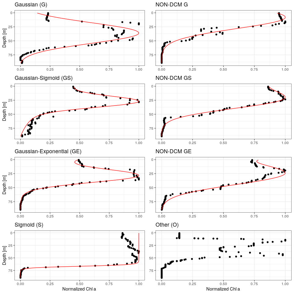
Figure 1 Examples of chl a profiles matched by each of the considered analytical forms. Right column: DCM profiles. Left column: non-DCM profiles discriminated by the ratio between surface and DCM chl a concentration (Sect. 3.2), and an example for the unmatched “other” category, which often corresponds to double chl a peaks.

2.4 Chl a sampling and float deployment

To validate the retrieval of chl a concentration from fluorometers in the Black Sea, a new BGC-Argo float (WMO 6903240) equipped with both chl a and CDOM fluorometers was deployed in the western Black Sea on 29 March 2018. Conjointly at the site of deployment, water samples were collected for chl a determination in the lab. This sampling took place on board the RV Akademik (Institute of Oceanology – Bulgarian Academy of Sciences) at a station localized at 43^∘10^′ N and 29^∘ E. Seawater samples were obtained using a CTD carousel equipped with twelve 5 L Niskin bottles. Samples were taken at 12 different depths between 1000 m and the surface and were considered to be co-located in time and space with the float deployment. Seawater samples were vacuum filtered through 47 mm diameter Whatman GF/F glass fibre filters (0.7 µm pore size). Filtered volumes varied between 4 L near the surface and approximately 5 L between 100 and 1000 m. After filtration, filters were immediately stored in liquid nitrogen and then at −80 ^∘C until HPLC analyses at the Villefranche Oceanographic Laboratory. These analyses were performed using the procedure from Ras et al. (2008) for the determination of chl a concentrations and other pigments. The first deep chl a profile taken by the float after deployment (during the descent) was used to retrieve chl a using the FDOM correction and compared with HPLC data. Only one HPLC profile was taken, strictly collocated at the deployment of the new float. It was not possible to take additional collocated HPLC profiles after the float was deployed. Therefore, we have to assume that the absence of chl a at depth, as shown by our unique HPLC profile, is valid at basin scale and at all times. This assumption is supported by the relative spatial uniformity of CDOM profiles (not shown).

2.5 Profile diagnostics

To characterize the chl a vertical distribution and its environmental context, we consider the following diagnostics.

• z_low locates the deepest penetration of chl a (> 0.01 mg m⁻³).

• z_50,bottom and z_50,up were derived as boundaries to the bulk of the chlorophyll content. Both were obtained by assessing the depth needed to obtain 75 % of total chl a content by vertical integration, going downward from the surface (z_50,bottom) and upward from 200 m (z_50,up). These boundaries thus locate the depth interval containing 50 % of the chl a content (hereafter referred to as the bulk of chl a content or the chl a bulk).

• z_DCM indicates the depth of the DCM.

• z_MLD indicates the depth of the MLD.

• z_PAR 1 % indicates the depth where in situ PAR reaches 1 % of its surface values.

The pycnal depths of diagnostics presented above are noted similarly using σ instead of z and obtained from interpolation of potential density anomalies at sampling depths.

2.6 Backscattering data and normalization

In order to evaluate the correspondence between chlorophyll and phytoplankton cells, we consider BBP data. This is the best proxy that can be obtained from the current Black Sea BGC-Argo dataset, although the complexity and variability of the Black Sea optical properties (Churilova et al., 2017) prohibit the establishment of a strict relationship between BBP and the abundance of phytoplanktonic cells. To compare the chl a and BBP values from many profiles despite the variability in vertical distribution and concentration, the chl a, BBP and depth of individual profiles are normalized as follows:

$$\begin{array}{}\text{(1)}& {\displaystyle }{z}_{\mathrm{norm}}={\displaystyle \frac{z-z_{\mathrm{MLD}}}{z_{\mathrm{DCM}}-z_{\mathrm{MLD}}}},\text{(2)}& {\displaystyle }\text{chl}{a}_{\mathrm{norm}}={\displaystyle \frac{\text{chl}a}{\text{chl}{a}_{\mathrm{DCM}}}},\text{(3)}& {\displaystyle }{\mathrm{BBP}}_{\mathrm{norm}}={\displaystyle \frac{\mathrm{BBP}}{{\mathrm{BBP}}_{max}}},\end{array}$$

where BBP_max is the maximum BBP value evaluated for each individual profile between the surface and 1.5 times z_DCM. The latter vertical restriction is considered to avoid the peak in BBP that is typically visible in the vicinity of the anoxic interface and is related to bacterial activity (Karabashev, 1995).

3 Results

3.1 Validation of the FDOM-based method in the Black Sea

In this section, HPLC data taken at deployment will be compared with successive levels of correction on chl a data: (1) no correction (raw data), (2) application of the correction factor of Roesler et al. (2017) for the Black Sea on raw data, (3) FDOM-based correction of Xing et al. (2017) and (4) NPQ correction, in order to validate the global correction of chl a profiles in the Black Sea.

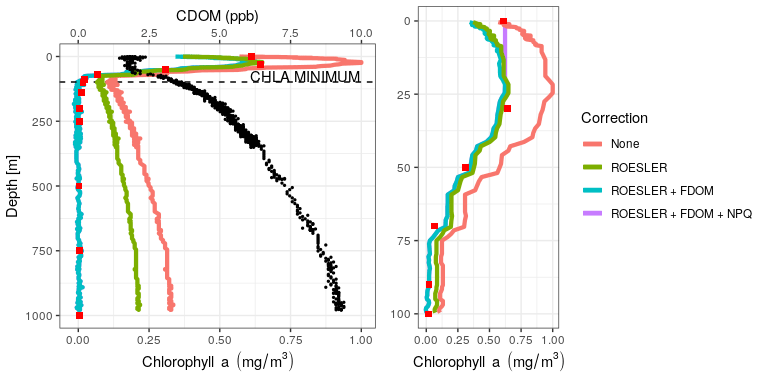
Figure 2 Vertical chl a profiles obtained at the deployment of the float 6903240 on 29 March 2018 at 49^∘10^′ N and 29^∘ E, using different levels of correction. HPLC data are depicted as red squares and CDOM as black dots. Right panel: zoom of the surface layer.

Firstly, HPLC data evidence the absence of chl a below a depth of 200 m (<0.01 mg m⁻³, ranging from 0.002 to 0.004 mg m⁻³). HPLC also provides insight into the planktonic communities (IOCCG, 2014). Here, we observed a dominance of diatoms with Fucoxanthin concentrations ranging from 0.13 to 0.16 mg m⁻³ in the 0–50 m range. Low abundances of dinoflagellates, prymnesiophytes, pelagophytes, cryptophytes and cyanobacteria were also observed in the 0–30 m range. The increase in the fluorescence signal (Fig. 2) that characterizes Black Sea chl a profiles is thus not associated with chl a but more likely results from the presence of high levels of CDOM as suggested by Xing et al. (2017).

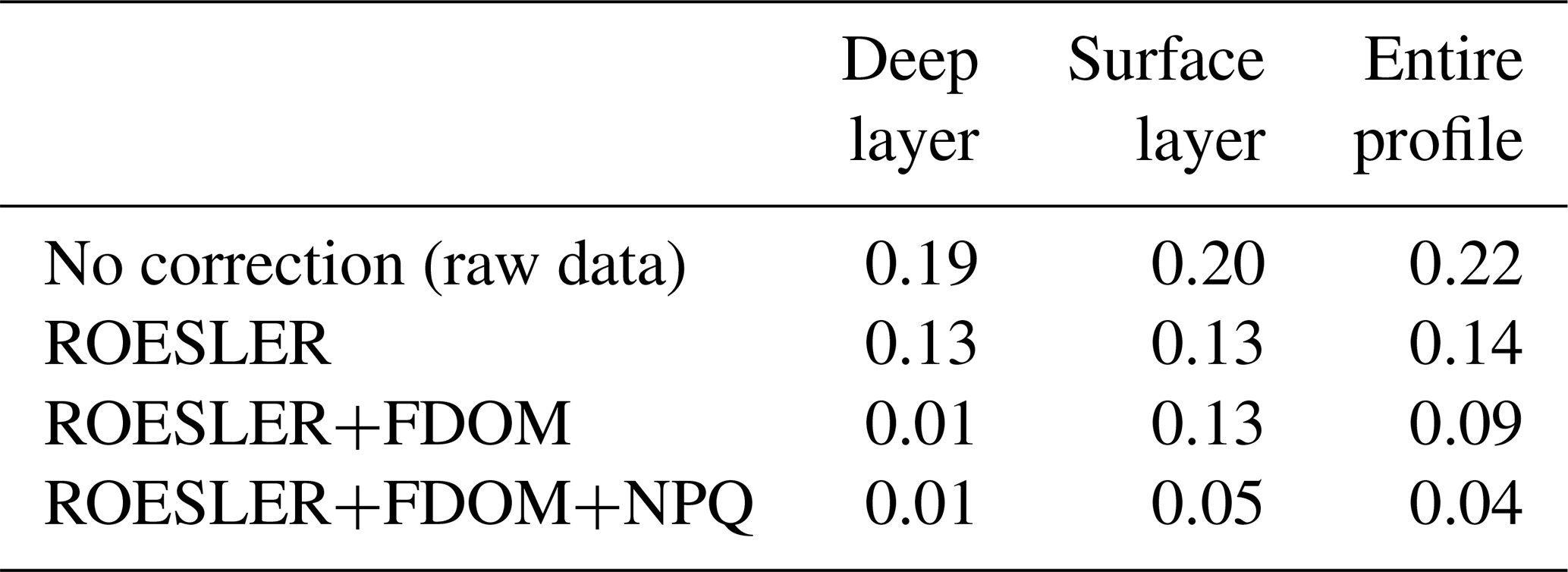
Then, a regional correction factor of 0.65 following the recommendation of Roesler et al. (2017) was applied to all data (results in Table 1) before using the FDOM-based correction. The shape of the chl a profile after the FDOM correction in the surface layer is questionable. Based on HPLC data, it seems that it displays a sigmoid shape. However, based on chl a not corrected for NPQ, it is qualified as a Gaussian–exponential with a $\frac{\text{chl}{a}_{\mathrm{DCM}}}{\text{chl}{a}_{\mathrm{surface}}}$ ratio of ∼ 1.8. Corrected for NPQ, the aforementioned algorithm qualifies it as a Gaussian–sigmoid but rejects it due to its ratio $\frac{\text{chl}{a}_{\mathrm{DCM}}}{\text{chl}{a}_{\mathrm{surface}}}$ of 1. This discrepancy highlights the importance of NPQ correction for daytime chl a profiles. However, a denser vertical sampling for the HPLC acquisition would have been needed to demonstrate the total absence of a subsurface chlorophyll maximum. In deeper waters, not affected by NPQ, the chl a minimum measured by the float (on the red curve, i.e. no correction) is located at 98.5 m (0.10 mg m⁻³) while the minimum non negligible value from discrete water samples (HPLC) is located at 140 m (0.01 mg m⁻³). Below that depth, chl a concentrations can be considered to be zero. In the deep layer (i.e. below the chl a minimum; see also Fig. 2), the RMSE¹ between chl a estimations obtained by HPLC (observations) and chl a retrieved from the ROESLER+FDOM chl a corrected profile (modelled values) is equal to 0.01 mg m⁻³ while the RMSE for raw data is 0.19 mg m⁻³. In the surface layer, the RMSE is equal to 0.13, 0.05 and 0.20 mg m⁻³ for the ROESLER+FDOM, the ROESLER+FDOM+NPQ and the uncorrected profiles, respectively. Therefore, we assume that the ROESLER+FDOM+NPQ correction is a consistent approach for chl a profiles in the Black Sea, and we use the notation chl a to denote $F_{\text{chl}a,\mathrm{ROESLER}+\mathrm{FDOM}+\mathrm{NPQ}}$ data for the rest of the paper.

Table 1 RMSE (mg m⁻³) comparison between HPLC measurements (i.e. 12 points; see Sect. 2.4 for more details) and chl a retrieved from Fluo using different levels of correction.

3.2 Categories of chl a profiles

Chl a profiles are firstly categorized according to the best-fitting analytical form (Fig. 3). Despite the use of a $R_{\mathrm{adj}}^{\mathrm{2}}$ metric, it seems that the plasticity of the Gaussian–sigmoid formulation provides a best fit in most cases. The best-fitting form can therefore not be used as a single criterion to discriminate DCM and non-DCM profiles, and individual profiles are further requested to have a chl a concentration at the DCM that is at least a third higher than at the surface to be tagged as DCM profiles. This criterion was chosen based on visual inspection, to filter out profiles wrongly tagged as DCM due to signal fluctuations near the surface. Non-DCM profiles dominate from November to March, while clear DCM dynamics set in from April to October. A complication arises in this DCM seasonal sequence when profiles categorized as others are counted as non-DCM profiles. Those profiles most often consist in double peaks (see example Fig. 1), which explains their rejection based on $R_{\mathrm{adj}}^{\mathrm{2}}$. Yet, all series of other profiles for any individual float are systematically preceded and followed by DCM forms. In the following, others are thus considered local perturbations of DCM structures (e.g. Mikaelyan et al., 2020) and counted among DCM profiles.

The non-DCM season is largely dominated by Gaussian–sigmoid forms. Pure exponential profiles are never observed. Pure sigmoid profiles, which denote a well-homogenized planktonic biomass in the surface layer, are observed from October to April with a clear peak in December–January, consistent with the known seasonality of the MLD in the Black Sea (e.g. Capet et al., 2014).

The DCM season opens mainly with Gaussian–sigmoid profiles. Later, Gaussian–exponential and finally simple Gaussian profiles are observed, which denote a successive depletion of the surface chl a content (Fig. 3).

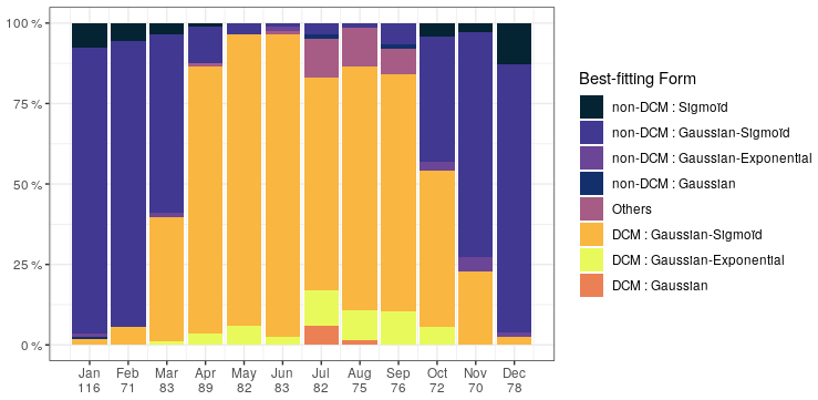
Figure 3 Percentage of best-fitting forms for chl a profiles for each month. Number of profiles is given on the horizontal axis.

No meaningful spatial pattern of the DCM period can be evidenced at first glance (Fig. 4) and both the beginning and end of the DCM season are consistent across the basin.

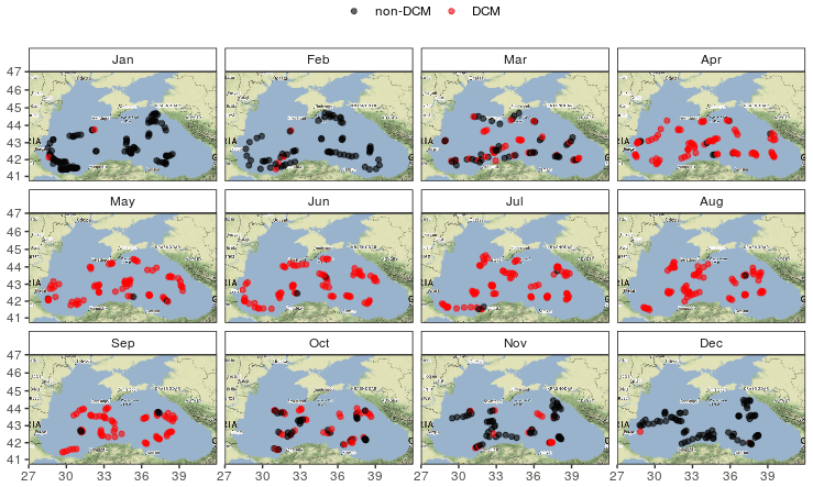
Figure 4 Monthly spatial distribution of DCM and non-DCM profiles indicates homogeneous DCM dynamics in the open basin. This map was created using tiles by Stamen Design, under CC BY 3.0 with data from © OpenStreetMap contributors 2020, distributed under a Creative Commons BY-SA License.

3.3 Seasonal variations in specific diagnostics of the chlorophyll distribution.

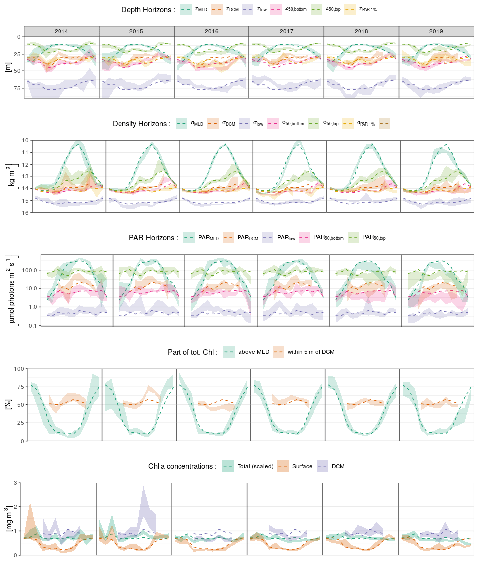
We present here the seasonal evolution of diagnostics (see Sect. 2.5) extracted from chl a profiles and their environmental context, using both vertical depth (Fig. 5a) and density (Fig. 5b) scales and considering the absolute irradiance observed at those layers (Fig. 5c). Diagnostics specific to the DCM are not considered from November to March, according to Sect. 3.2.

In winter, the mixed layer reaches a mean depth of 35 m and extends over the entire euphotic zone (defined by the 1 % of surface incoming PAR, Fig. 5a). The deepest chl a records are found near 70 m, but most of the chlorophyll content is located within the mixed layer. Accordingly, the lower bulk boundary, z_50,bottom, coincides with z_MLD. By definition, density is homogeneous within the mixed layer, at a mean value of 14 kg m⁻³, and the density scale only reveals that some chl a content is still observed within the upper pycnocline, slightly above the 15 kg m⁻³ density layer (Fig. 5b). A similar situation lasts for December, January and February.

In March, z_MLD decreases with the progressive onset of stratification. The upper boundary of the bulk chl a content evolves slightly downwards, with a progressive appearance of DCM profiles (Fig. 3). In April, all depth diagnostics of the chl a distribution migrate downward, together with the euphotic depth. At the same time, the absolute PAR observed at those horizons remains relatively unchanged (Fig. 5c). Deep chl a records are observed at 80 m, which is the annual maximum. The DCM is now firmly formed at a depth of about 40 m. From April to May, the DCM remains close to the lower bulk boundary, and the chl a vertical distribution presents a notable downward skewness. In particular the DCM is recorded at relatively low absolute irradiance levels, on average below 10 µmol photons m⁻² s⁻¹. On a density scale, σ_50,bottom is observed near the layer of the winter σ_MLD, and a collocation between σ_DCM and σ_50,bottom persists until May.

In June, the vertical chl a distribution shifts towards a structure that remains stable during the months of July and August. During this period, the DCM depth is sensibly shallower (30 m) than during the DCM formation months. The median value of z_DCM is now clearly distinguished from that of z_50,bottom, and the skewness in the vertical chl a distribution is weaker. The DCM is also found at a higher PAR value than during the period of April–May (Fig. 5c). Conversely, the PAR values at z_50,top, z_50,bottom and z_50,low remain practically unchanged during the entire year. From June to August, the bulk chl a progressively narrows around z_DCM (see z_50,bottom and z_50,top, Fig. 5a) and remains located well below z_MLD.

In September, the thermocline starts to weaken. Conversely to what was observed between March and April, z_50,top, z_50,bottom and z_low migrate upward, together with the euphotic depth, while they remain at a similar location in terms of PAR. On a density scale, it appears that σ_50,bottom still remains at its previous location, while the upper boundary σ_50,top is lifted up to lighter layers and presents an important variability. In October, the deepening MLD reaches the upper part of the bulk chl a. An important decrease occurs in the proportion of DCM profiles (Fig. 3): this is the end of the DCM season.

Interestingly, the position of the deepest chl a records is remarkably stable along the season in terms of absolute irradiance and hence undergoes seasonal variations in depth coordinates as the surface incoming irradiance increases in summer. On a density scale, it just overlays the nitracline level, located at 15.5 kg m⁻³ by Konovalov et al. (2006).

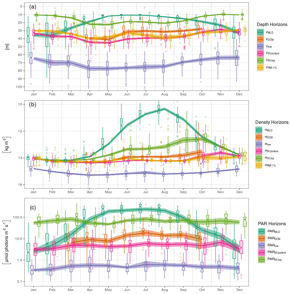
Figure 5 Seasonal variations in the position of horizons characterizing the chl a vertical distribution and its environment on (a) depth, (b) density and (c) PAR irradiance scales. Box plots indicate monthly medians and interquartile ranges. Continuous lines indicate monthly means and their 95 % confidence interval (shaded area, bootstrap estimates). While box plots are slightly shifted horizontally to avoid overlapping, the means are all centred on the monthly grid.

3.4 Chl a concentrations and vertically integrated content

Here, we consider seasonal variations in chl a concentrations at the surface, at the DCM and in the total chl a content, i.e. the concentration integrated over the vertical. In the following, the total chl a content is scaled by a constant depth of 40 m to reach units of volumetric concentration (mg m⁻³). The arbitrary scale of 40 m corresponds to the mean of z_50,bottom.

Ranging between 0.5 and 2 mg m⁻³ (i.e. 20 and 80 mg m⁻²), the total chl a content only presents weak seasonal variations with a maximum in March (Fig. 6a). Surface chlorophyll concentration, instead, has a marked seasonal variability and decreases by a factor of 2 to reach 0.35 mg m⁻³ from April to September, while chl a concentrations at the DCM are generally close to 0.8 mg m⁻³ in this period and reach mean values above 1 mg m⁻³ in August. To summarize, roughly 80 % of the total chl a content is contained within the MLD in winter, while this ratio falls to 10 % during the DCM season (Fig. 6b). In summer, about 50 % of the total content can be found within a 10 m layer surrounding the DCM, a value that peaks in August and reaches 80 % in some cases.

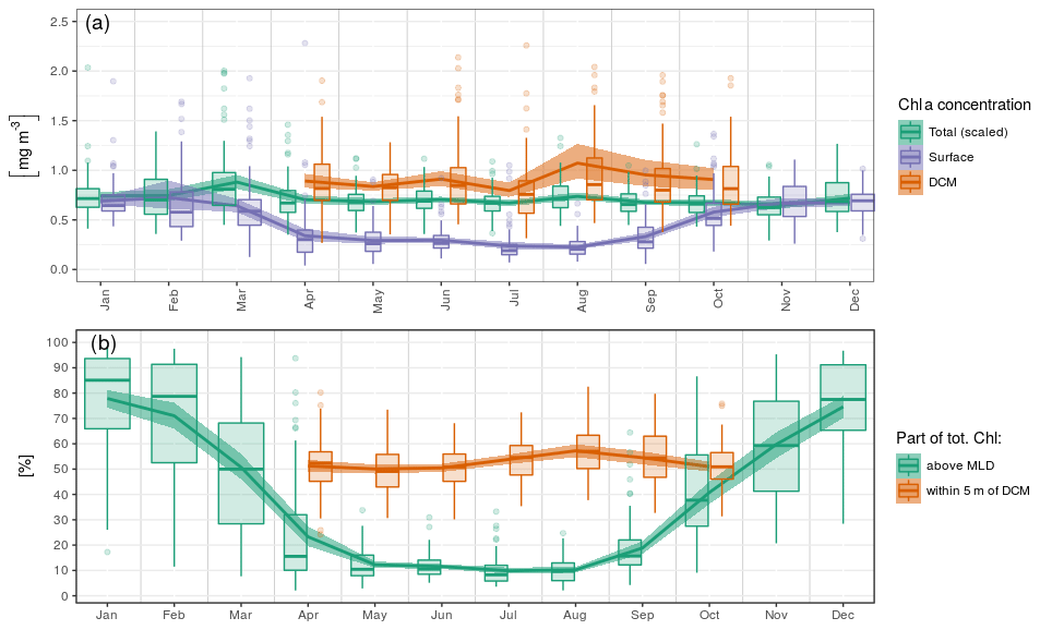
Figure 6 Seasonal variations in (a) surface, DCM and total chl a concentrations and (b) relative parts of the total chl a content around specific horizons. The total chl a concentration in (a) is the vertical integral of chl a concentration scaled by a constant depth of 40 m to reach the unit of volumetric concentrations (mg m⁻³).

For the interested readers, we propose in Appendix C the interannual equivalent of Figs. 5 and 6, although we decided to concentrate this study on describing a typical seasonal cycle, considering that the data were too scarce to support a reliable interannual analysis.

3.5 Normalized chlorophyll and backscattering profiles

We analyse here the chl a and BBP values for DCM profiles only. In particular, we seek for an eventual correspondence between local maxima in chl a and BBP at z_DCM, or a vertical shift in the position of these maxima, in order to characterize the nature of the DCM. Indeed, a chl a profile such as recorded by BGC-Argo floats only reflects the product between a profile of planktonic biomass and a profile of their cellular chl a content. It is only considered per se for the reason that it is easily measurable.

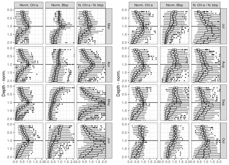
In order to provide a general overview of all profiles despite their disparity in terms of DCM depths and concentrations, a normalized referential was used to build Fig. 7 (see Sect. 2.6 for a description of the normalization procedure). The fact that narrow maxima of chl a are depicted at the normalized depth of 1, which is defined on the basis of the calibrated Z_max parameter of the best-fitting analytical forms (Appendix B), simply confirms the reliability of the approach considered to characterize the DCM, i.e the classification protocol and the use of parameters issued from their calibration.

A well-defined maximum in BBP can be seen at the DCM depth in March. A similar local maximum in BBP profiles can also be seen close to the DCM reference depth for other months but never as clearly as for the month of March.

The ratio between normalized BBP and chl a value then evidences an important difference between the two phases of the DCM period described in Sect. 3.3. During the first phase of the DCM period (April–May), a peak in this ratio is clearly visible at the DCM depth, while from June and during the second phase (July–September) the peak in the chl a ∕ BBP ratio is found below the DCM depth.

Figure 7 Distribution of normalized chl a and BBP values for different layers of normalized depth. The depth is normalized for each profile so that values of 1 and zero correspond to the depths of DCM and MLD, respectively (see Sect. 2.6 for the normalization procedure).

4 Discussion

4.1 Using BGC-Argo to decipher the Black Sea DCM dynamics

The spatial distribution of BGC-Argo data in the Black Sea is presently incomplete and opportunistic. In addition, in the Black Sea BGC-Argo floats tend to exclude areas characterized by divergent flows such as the shelf regions or the centres of the two central gyres. However, the Argo sampling protocol permits regular seasonal sampling of the central basin, which constitutes an important asset compared to traditional cruise-based datasets, and provides a satisfactory number of observations for seasonal analysis (numbers of profiles for each month are given in Fig. 3). Furthermore, the dense vertical sampling obtained from BGC-Argo floats permits a refined characterization of DCM depth and density diagnostics.

At present BGC-Argo floats only provide limited proxies to evaluate the relationships between chlorophyll content and phytoplankton biomass, which is essential to upscale the present analysis to larger-scale considerations such as productivity and carbon sequestration issues. However, the fact that the first DCM profiles in March correspond to a clear maximum in BBP (Fig. 7) suggests that the DCM is also initiated as a peak in phytoplankton biomass and not only as a local increase in the chlorophyll cellular content, as suggested by Finenko et al. (2005).

In the first phase (April–May), no clear vertical shift can be seen between the (normalized) profiles of chl a, BBP and their ratio. In the second phase (July–September), however, a maximum in the chl a ∕ BBP ratio is clearly seen below the DCM depth, which is similar to the theoretical profiles of Fennel and Boss (2003) that describe the imprint of photoacclimation mechanisms on the vertical distribution of phytoplankton biomass and their chl a content. This important difference between the two phases of the DCM periods suggests that the influence of photoacclimation mechanisms on the shapes of chl a profiles evolves seasonally, which nuances the conclusions of Finenko et al. (2005). Furthermore, according to Fennel and Boss (2003), it suggests that a subsurface maximum in planktonic biomass may exist above the DCM during the second phase.

Figure 7 shows high BBP values in the upper part of the normalized scale (i.e. between z_MLD and z_DCM) that are not mirrored in the chl a records. This vertical discrepancy may indicate (1) the presence of non-phytoplanktonic particles in the upper layers, (2) larger cellular chl a content in phytoplankton located around the DCM, and/or (3) an important difference in terms of phytoplanktonic communities and in particular in terms of cell size. The known disparity in species dominance between surface and subsurface waters (Mikaelyan et al., 2020), in particular regarding the size of dominant species, prevents consideration of a strict relationship between particle backscattering and planktonic biomass, so that we cannot argue for one or another of the above propositions. However, the peak in BBP that is visible near the DCM depth for several months supports the hypothesis that the DCM does, to some substantial extent, correspond to a local peak in planktonic biomass.

BGC-Argo floats thus provide evidence for clear seasonal DCM dynamics that prevail over the entire central Black Sea, with almost all profiles categorized as DCM from April to September (Fig. 3). This suggests the existence of two distinct phases during which the relationship between chl a and phytoplankton biomass differs. During this period, the DCM concentrates about 45 %–65 % (and up to 80 % in some specific cases) of the total chl a content inside a 10 m layer located from 40 to 30 m below the surface, where local PAR irradiance ranges from 4 to 15 and from 10 to 20 µmol photons m⁻² s⁻¹ for the first (April–May) and second (July–September) phases, respectively (reporting first and third quartiles).

These DCM depth estimates are deeper than those previously reported by Finenko et al. (2005), but the lack of overlapping data precludes an association with either methodological factors or interannual variability. One could consider, however, the fact that both Yunev et al. (2005) and Finenko et al. (2005) used a single analytical form (modified Gaussian) to characterize chl a distribution as a function of depth during the DCM season. In particular, to ignore the distinction between DCM and non-DCM profiles may considerably bias DCM diagnostics estimates.

4.2 Considering horizontal variability in the different vertical coordinate systems

Both Yunev et al. (2005) and Finenko et al. (2005) considered depth coordinates to characterize the vertical distribution of chl a during the DCM period. Yunev et al. (2005) completed their analysis by assessing, for each considered profile, the depth of the 16.2 kg m⁻³ isopycnal, in order to characterize subregions (or “hydrodynamic regimes”) of the central Black Sea. The authors concluded that z_DCM can be considered independent from hydrodynamic regimes, which amounts to saying that depth diagnostics are sufficiently consistent across the basin to serve as the basis for an interannual trend analysis. On the contrary, Finenko et al. (2005) highlighted the variability of z_DCM and its relationship with the surface chl a content, as the authors aimed to identify a general formulation to retrieve the vertically integrated biomass from remote sensing surface observations. The authors did not further comment on the spatial structure of the DCM diagnostics.

No clear spatial pattern emerges from the analysis of the DCM depth diagnostics, and Fig. 4 highlights that the seasonality of the DCM dynamics is consistent over the entire central basin. In this regard the Black Sea differs from the Mediterranean Sea, where clear longitudinal gradients in environmental conditions (nutrients and light) induce spatial gradients for DCM characteristics, visible all along the DCM period (Letelier et al., 2004; Mignot et al., 2014; Lavigne et al., 2015).

Nevertheless, the open Black Sea does present a major spatial structure which lies in the general curvature of isopycnals: layers of equal density are dome-shaped and significantly shallower in the centre than in the periphery (Murray et al., 1991). In addition, isopycnals undergo vertical displacement at timescales from hours (internal waves, inertial oscillations scale at about 17 h in the Black Sea; e.g. Filonov, 2000) to weeks (eddies and mesoscale dynamics; Stanev et al., 2013). This leads many authors to use density, rather than depth, as a vertical coordinate system (Tugrul et al., 1992) in order to minimize the spread of vertical diagnostics characterizing layers that are mostly maintained by isopycnal diffusion, such as the nitracline and oxycline depths. Here, the spread of monthly diagnostics is depicted by the interquartile ranges in Fig. 5 and mainly derives from interannual and/or horizontal variability. We assume that a seasonal change in the spread of the position of specific horizons, presented on depth, density or irradiance scales, can be exploited to decipher which driving factors rule the development and structure of DCM dynamics in the Black Sea.

4.3 Drivers of the seasonal DCM dynamics

It is remarkable that the irradiance values recorded at z_50,top, z_50,bottom and z_low are essentially constant over the seasonal cycle. The seasonal vertical displacement of those horizons on a depth scale may thus be associated with the seasonal variation in the surface incoming radiation, which is significant at the latitudes of the Black Sea. Such a simplified description does not hold, however, for z_DCM, which we detail as follows.

During winter, the MLD extends beyond the euphotic depth (Fig. 5a). The appearance of a DCM at the base of the MLD, when it is shoaling at the end of winter, is thus in agreement with the general Sverdrup theory (and its extensions described in the introduction).

During the first phase of the DCM season (April–May), the DCM remains close to the density layer that corresponds to the winter MLD. Following Navarro and Ruiz (2013), this is highlighted by the ratio obtained between individual σ_DCM values and σ_MLD,max, i.e. the maximum σ_MLD value registered by the same float in the same year (Fig. 8). This ratio is close to unity during the first phase of the DCM period, regardless of spatial or interannual variability, which clearly indicates that the depth of initial DCM settlement is ruled basin-wide by the vertical extent of the winter MLD and that this initial location holds for at least 2 months. Note that the spread of PAR_DCM (Fig. 5c) is large during this first phase, which further supports the hypothesis for density-related driving factors in setting the vertical position of the DCM.

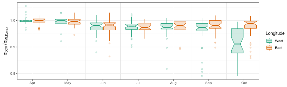
Figure 8 Ratio between the σ_DCM of individual profiles and the maximum σ_MLD recorded by the same float during the same year. West and east longitude are defined with respect to the meridian of 34.5^∘ E.

Obviously, fast biomass regeneration occurs within the DCM. The standing DCM thus results from a balance between growth, loss and transport terms that respond to environmental factors, i.e. mainly nutrient fluxes from below, light fluxes from above, density gradients and grazing pressure (Cullen, 2015). But the environment to which these terms respond is shaped by the presence of the DCM. For instance, accounting for light attenuation by phytoplankton and nutrient recycling upon cellular decay provides mechanistic explanations for such “bending forces” (e.g. Klausmeier and Litchman, 2001; Beckmann and Hense, 2007). The fact that such mechanisms induce hysteresis in the pycnal position of the DCM and that this is the most likely explanation for the high concordance between density DCM position and density reached by winter MLD is essentially the message of Navarro and Ruiz (2013). Our results concur with this description for the first phase of the DCM period, during which BBP profiles also suggest that photoacclimation mechanisms have not yet induced a substantial structure in the BBP-to-chl a ratio (Sect. 4.1).

We then observe in June a shift towards a different DCM structure that holds from July to September. This shift involves (i) a decoupling between particle backscattering (our best proxy for biomass; Fig. 7) and chlorophyll profiles and the establishment of a maximum in the chl a ∕ BBP ratio below the DCM, which suggests impacts of photoacclimation mechanisms on the DCM structure (Fennel and Boss, 2003); (ii) the appearance of pure Gaussian profiles (Fig. 3), implying depletion of surface chl a content; (iii) an upward displacement of the DCM, on both depth and pycnal scales (Fig. 5a, b) and an upward displacement of the DCM in terms of the irradiance scale (Fig. 5c), from about 4–15 to about 10–20 µmol photons m⁻² s⁻¹; (iv) a decrease in the spread of the irradiance value at the DCM (see the interquartile ranges in Fig. 5c); and (v) a gradual increase (peaking in August) in chl a concentration at the DCM (Fig. 6a) and in the proportion of total chl a content that is located around the DCM (Fig. 6b).

The fact that this shift occurs at the time of the year when surface irradiance is maximal and opposes the expected responses to increased surface incoming irradiance (i.e. a downward displacement of the DCM; Beckmann and Hense, 2007) suggests an important role of biotic factors in reshaping the vertical distribution of chl a, e.g. species succession in phytoplanktonic population (Mikaelyan et al., 2018) and/or changes in grazing pressure or a substantial seasonal increase in the upward nutrient supply. We tend to favour the lead of biotic factors, since seasonal assessment of the vertical turbulent transport in the Black Sea points towards a decrease in diapycnal diffusion during the warm period (Podymov et al., 2020) which, again, would bring the DCM downward. However, these are hypotheses that we do not have the means to confirm on the basis of the considered dataset.

In October, as the DCM season ends, spread in σ_DCM (Fig. 5b) and PAR_DCM (Fig. 5c) largely increases. For the first time in the year, a clear spatial differentiation occurs as the DCM evolves away from the density layer of the winter MLD, significantly more in the western basin than in the east (Fig. 8). This indicates that, upon closure of the DCM season, the environmental conditions that drive the DCM upward are affected by a significant spatial variability. A likely explanation for this longitudinal difference lies in the fact that lateral nutrient inputs are enhanced in the western part of the basin by the proximity of the northwestern shelf system. We thus suggest that lateral nutrient inputs trigger this spatial disparity in the very last months of the DCM season, which concurs with the fact that nutrient export from the northwestern shelf to the open sea has been evaluated to be maximal in October (Grégoire and Beckers, 2004).

Ultimately, model studies would be required to test different hypotheses on the driving forces of DCM dynamics and to make comparisons with those identified in other parts of the world considering in particular, the neighbouring Mediterranean Sea (Terzić et al., 2019).

5 Conclusions

In this study, we use BGC-Argo data (2014–2019, about 1000 profiles) to characterize the vertical distribution of chl a in the Black Sea. We first highlight the importance of processing raw fluorescence data obtained from BGC-Argo floats to obtain accurate chl a estimates, which involves (i) a sensor correction (Roesler et al., 2017); (ii) a correction for CDOM fluorescence as proposed by Xing et al. (2017) and (iii) non-photochemical quenching as proposed by Xing et al. (2012). While the above procedures are validated on the basis of an HPLC in situ profile, we suggest that further in situ HPLC datasets should be consolidated in order to fine-tune corrections of BGC-Argo Fluo measurements in the Black Sea.

The processed chl a dataset is then used to characterize seasonal changes in the vertical distribution of chl a and to discuss the mechanisms that underlie the DCM dynamics. Our analyses reveal DCM dynamics that dominate chl a distribution from April to October over the entire central basin, in agreement with previous studies (Yunev et al., 2005; Finenko et al., 2005). While Yunev et al. (2005) considered that DCM depth diagnostics were sufficient to infer long-term trends from limited datasets, the detailed vertical sampling provided by BGC-Argo floats and the use of refined analytical forms to distinguish between DCM and non-DCM profiles allowed us to demonstrate (i) that a significant variability affects DCM diagnostics when expressed on a depth scale and (ii) that the DCM season can be divided into two phases with distinct driving mechanisms. Our analysis indeed indicates that, during the first phase (April–May), the DCM remains attached to the density layer reached by the winter maximum MLD. This concurs with the hysteresis hypothesis proposed by Navarro and Ruiz (2013), in which the DCM is seen as a self-sustaining structure that influences its surrounding environment, rather than a local maximum adapting instantaneously to external factors. During the second phase (July–September), we suggest that biotic factors are responsible for an upward displacement of the DCM structure, visible in depth, density and irradiance scales, since increased surface irradiation and reduced diapycnal mixing at the pycnocline would normally induce a downward displacement. On average, the DCM concentrates about 50 % (55 %) of the total chl a content within a 10 m layer centred at a depth of about 40 m (30 m) for the first and second phases, respectively. It is only towards the end of the thermocline season (October) that the disturbed DCM structure indicates a substantial spatial gradient, which we suggest is structured by the enhanced lateral inputs of nutrients in the western region.

At present the Black Sea BGC-Argo dataset does not allow us to establish a strict relationship between chl a and planktonic biomass. The DCM is clearly associated with an increase in intra-cellular chlorophyll content at depth during the second phase, which shows the typical signatures of photoacclimation mechanisms (Fennel and Boss, 2003). However, the presence of local peaks in BBP profiles at the DCM depth suggests that the DCM can also be associated with peaks in biomass.

This study highlights the importance of considering DCM dynamics in assessments of Black Sea productivity. In order to further appreciate its interannual variability and to strengthen the extrapolation from chl a to actual biomass and productivity we encourage continuous support and enrichment of the Black Sea BGC-Argo fleet in terms of both the number of floats and equipped sensors.

Appendix A: FDOM method

$$\begin{array}{}\text{(A1)}& \begin{array}{rl}\mathrm{FChl}{a}_{\mathrm{cor}}& =\mathrm{FChl}{a}_{\mathrm{meas}}-\mathrm{FChl}{a}_{\mathrm{dark}}\\ & -{\mathrm{Slope}}_{\mathrm{FDOM}}\cdot ({\mathrm{FDOM}}_{\mathrm{meas}}-{\mathrm{FDOM}}_{\mathrm{dark}}),\end{array}\end{array}$$

where FChl a_cor is the corrected chl a obtained by removing from the measured chl a (FChl a_meas) the sensor bias (FChl a_dark, dark signal measured in the absence of chl a) and the contribution from CDOM estimated as proportional (coefficient Slope_FDOM) to the amount of CDOM estimated as the measured CDOM (FDOM_meas) corrected for the sensor bias (FDOM_dark). All values are obtained after conversion from Fluo values (in voltage or digital counts) with parameters provided by the manufacturer of each sensor, in milligrammes per cubic metre for chl a and in parts per billion for CDOM. Slope_FDOM represents the ratio between the fluorescence of CDOM measured by a chl a and a CDOM fluorometer. This ratio is assumed to be constant over depth and its units are given in mg m⁻³ ppb⁻¹.

Below a certain depth, FChl a_cor should be zero and hence Eq. (A1) gives

$$\begin{array}{}\text{(A2)}& \begin{array}{rl}\mathrm{FChl}{a}_{\mathrm{meas}}& =\mathrm{FChl}{a}_{\mathrm{dark}}+{\mathrm{Slope}}_{\mathrm{FDOM}}\\ & \cdot ({\mathrm{FDOM}}_{\mathrm{meas}}-{\mathrm{FDOM}}_{\mathrm{dark}}).\end{array}\end{array}$$

That can also be written as

$$\begin{array}{}\text{(A3)}& \mathrm{FChl}{a}_{\mathrm{meas}}={\mathrm{Slope}}_{\mathrm{FDOM}}\cdot {\mathrm{FDOM}}_{\mathrm{meas}}+\mathit{\alpha },\end{array}$$

where $\mathit{\alpha }=\mathrm{FChl}{a}_{\mathrm{dark}}-{\mathrm{Slope}}_{\mathrm{FDOM}}\cdot {\mathrm{FDOM}}_{\mathrm{dark}}$.

α is a constant bias that results from factory calibration error. Equation (A3) shows that Slope_FDOM and α can be retrieved with a linear regression in the depth range where FChl a_meas is expected to be zero due to the – assumed – absence of chl a. This depth range starts at the chl a minimum down to the bottom of the profile. In all investigated profiles, the chl a minimum is always deeper than the MLD or the DCM during the stratified season and never below 400 m; thus the determination of the depth range for the linear regression is easier than in Xing et al. (2017). Once Slope_FDOM and α are known, the profile can be corrected according to Eq. (A1).

Appendix B: Analytical forms of chl a profiles

Chl a profiles were fitted with the following analytical forms: (a) sigmoid, $F\left(z\right)=\frac{F_{\mathrm{surf}}}{\mathrm{1}+e^{(Z_{\mathrm{1}/\mathrm{2}}-z)s}}$ with F_surf, the chl a surface concentration, Z_1∕2 the depth at which the chl a concentration is half the chl a concentration at the surface and s the proxy of the sigmoid fit slope at Z_1∕2; (b) exponential, $F\left(z\right)=F_{\mathrm{surf}}{e}^{-\frac{\ln \mathrm{2}}{Z_{\mathrm{1}/\mathrm{2}}}\cdot z}$; (c) Gaussian, $F\left(z\right)=F_{max}{e}^{-\frac{(z-Z_{max}{)}^{\mathrm{2}}}{{\mathrm{dz}}^{\mathrm{2}}}}$ with F_max, the maximum chl a value; Z_max, the depth of the DCM; and dz, the proxy of the Gaussian fit thickness; (d) Gaussian–exponential, $F\left(z\right)=F_{\mathrm{surf}}{e}^{-\frac{ln\mathrm{2}}{Z_{\mathrm{1}/\mathrm{2}}}\cdot z}+F_{max}{e}^{-\frac{(z-Z_{max}{)}^{\mathrm{2}}}{{\mathrm{dz}}^{\mathrm{2}}}}$; (e) Gaussian–sigmoid, $F\left(z\right)=\frac{F_{\mathrm{surf}}}{\mathrm{1}+e^{(Z_{\mathrm{1}/\mathrm{2}}-z)\cdot s}}+F_{max}{e}^{-\frac{(z-Z_{max}{)}^{\mathrm{2}}}{{\mathrm{dz}}^{\mathrm{2}}}}$.

The initial parameters used before the fitting procedure were chosen based on the observed profiles. F_surf was chosen to be the mean chl a value in the MLD, and Z_1∕2 was chosen as the depth where F_surf was divided by 2 or replaced by the MLD if the MLD was deeper than Z_1∕2. Z_max and F_max followed their definition while dz and s were initially fixed at, respectively, 5 m and −0.01 m⁻¹. In this configuration, the algorithm converged in most cases.

Appendix C: Interannual variability

Analysing the interannual variability of the DCM seasonal sequence on the basis of the BGC-Argo dataset is difficult. First, because the dataset only expands over 5 years. Second, because subsetting the data per year gives even more place to the artefacts induced by uneven spatial sampling, the latter being particularly relevant for 2014 (∼ max 10 profiles per month).

Yet, to give a general appreciation of the stability of the DCM seasonal dynamics, Fig. C1 provides the specific annual expressions of the seasonal dynamics illustrated in Figs. 5 and 6.

The most striking feature is the relative stability of the DCM seasonal cycle. Although some years do present some notable anomalies with respect to the average seasonal cycle, no clear systematic implications could be drawn from this limited dataset. Questioning the drivers of interannual variability of the seasonal DCM dynamics is thus left for further studies. We redirect the interested reader to such a corresponding recent analysis proposed by Kubryakova and Kubryakov (2020).

Figure C1 Interannual variability (year-specific monthly medians and confidence interval; shaded area) depicted with year-averaged monthly medians (dotted lines) for the variables presented in Figs. 5a, b, c and 6a, b.