Technical note: A universal method for measuring the thickness of microscopic calcite crystals, based on bidirectional circular polarization

Coccoliths are major contributors to the particulate inorganic carbon in the ocean that is a key part of the carbon cycle. The coccoliths are a few micrometres in length and weigh a few picogrammes. Their birefringence characteristics in polarized optical microscopy have been used to estimate their mass. This method is rapid and precise because camera sensors produce excellent measurements of light. However, the current method is limited because it requires a precise and replicable set-up and calibration of the light in the optical equipment. More precisely, the light intensity, the diaphragm opening, the position of the condenser and the exposure time of the camera have to be strictly identical during the calibration and the analysis of calcite crystal. Here we present a new method that is universal in the sense that the thickness estimations are independent from a calibration but result from a simple equation. It can be used with different cameras and microscope brands. Moreover, the light intensity used in the microscope does not have to be strictly and precisely controlled. This method permits the measurement of crystal thickness up to 1.7 µm. It is based on the use of one left circular polarizer and one right circular polarizer with a monochromatic light source using the following equation:

$$d={\displaystyle \frac{\mathit{\lambda }}{\mathit{\pi }\mathrm{\Delta }n}}\arctan \left(\sqrt{{\displaystyle \frac{I_{\mathrm{LR}}}{I_{\mathrm{LL}}}}}\right),$$

where d is the thickness, λ the wavelength of the light used, Δn the birefringence, and I_LR and I_LL the light intensity measured with a right and a left circular polarizer. Because of the alternative and rotational motion of the quarter-wave plate of the circular polarizer, we coined the name of this method “bidirectional circular polarization” (BCP).

1 Introduction

Coccolithophores are abundant oceanic single-cell algae that produce calcite plates called coccoliths that are arranged around the cell to form an exoskeleton. Coccolithophores are extremely abundant in the whole ocean (Okada and Honjo, 1973), and some species form blooms that are detected by satellite imagery (Holligan et al., 1993). The coccoliths are major contributors to the particulate inorganic carbon (i.e. PIC) in the pelagic ocean (Milliman and Droxler, 1996; Suchéras-Marx and Henderiks, 2014), which is a key part of the carbon cycle. They are important contributors to the carbonate counter pump (Ridgwell and Zeebe, 2005), and they are considered climate stabilizers on long timescales (Zeebe and Westbroek, 2003; Höning, 2020). The calcite mass of the coccolith is therefore a parameter that is important to estimate for example to monitor the effect of ocean acidification on calcification (e.g. Beaufort et al., 2007, 2011) or to calculate their flux to the seafloor (Beaufort and Heussner, 1999). The coccoliths are so minute (few micrometres in length) and light (a few picogrammes) that they can be weighed individually only with extreme labour and expensive equipment (Hassenkam et al., 2011; Beuvier et al., 2019). Alternatively, the birefringence characteristics of coccoliths in polarized optical microscopy have been used to estimate their mass (Beaufort, 2005; Beaufort et al., 2014; Bollmann, 2014; Fuertes et al., 2014). The justification for measuring birefringence is that it directly relates the colour (and brightness) of a crystal observed under cross-polarized light microscopy to its thickness. The conversion comes without having to manipulate the particle. Moreover, this method is rapid and precise. The camera sensor produces excellent measurement of the light that travels through the polarizers and a calcite crystal which is converted into a thickness value and mass when it is associated with the surface measurement. The thickness estimation made by this method has been recently positively evaluated by the independent measurements made by X-ray tomography at the European Synchrotron Radiation Facility (ESRF) (Beuvier et al., 2019). The equipment needed for the measurements of the thickness is an optical microscope, with a pair of polarizers, a condenser, a high-resolution lens (X100 in our case) and a numerical camera. A precise calibration of the brightness of the microscope is required. The precision and stability of the microscope tuning constitute a limitation of the method. The light intensity, the diaphragm opening, the position of the condenser and the exposure time of the camera have to be strictly identical between the calibration and the analysis of the calcite crystal. Slight change in one of those parameters has important consequence for the results. Another limitation is that the measured light intensity is not linearly proportional to the thickness but follows a sigmoid (Beaufort et al., 2014; Bollmann, 2014), making it difficult to estimate the thickness precisely at the two ends of the calibration. The use of standard polychromatic “white” light induces a small imprecision, because the temperature of light that depends on the microscope – some have a bluish light and others have more yellowish light – will slightly change the result if not calibrated. There is a theoretical limit of the thickness estimation to about 1.56 µm when using a black and white camera. Some species have coccoliths thicker than this limit: in present ocean and Pleistocene sediments, rare examples are Coccolithus pelagicus, Ceratolithus cristatus and Pontosphaera multipora, and coccoliths exceed this threshold only on limited surfaces of the thickest specimens. This threshold is achieved more commonly in the Paleogene, for example with Reticulofenestra bisecta or Chiasmolithus grandis. The estimation of calcite particles thicker than 1.56 µm needs to be done with a colour camera with several calibration equations (Beaufort et al., 2014; González-Lemos et al., 2018). Here we propose a new method that solves those problems: the estimations are not the results of a calibration; they can be applied to crystals as thick as 1.7 µm and are not dependent on the precise tuning of the light of the microscope.

2 Principles

The representation of the polarized light is based on Jones's calculus (Jones, 1941). The microscope is composed of two circular polarizers – one left oriented and the other right oriented – used alternatively and one circular analyser.

2.1 Jones matrices

For an anisotropic material having its ordinary neutral axis horizontally, the Jones matrix is given by

$${\mathbf{W}}_{\mathrm{0}}=T\left[\begin{array}{ll}\mathrm{1}& \mathrm{0}\\ \mathrm{0}& (\mathrm{1}-n)e^{i\mathit{\varphi }}\end{array}\right],$$

where T is the (complex) transmission coefficient, η is the diattenuation and ϕ is the retardation, with $\mathit{\varphi }=\frac{\mathrm{2}\mathit{\pi }}{\mathit{\lambda }}\mathrm{\Delta }nd$ (where λ is the wavelength, Δn is the birefringence and d is the thickness).

If the neutral axis is rotated by an angle θ, the Jones matrix becomes

$${\mathbf{W}}_{\mathit{\theta }}=\mathbf{R}(-\mathit{\theta }){\mathbf{W}}_{\mathrm{0}}\mathbf{R}\left(\mathit{\theta }\right),$$

where R(θ) is the rotation matrix.

$$\mathbf{R}\left(\mathit{\theta }\right)=\left[\begin{array}{ll}\cos \mathit{\theta }& \sin \mathit{\theta }\\ -\sin \mathit{\theta }& \cos \mathit{\theta }\end{array}\right]$$

2.2 Proposed measurement scheme

Assuming that η=0 (no diattenuation), the input field is left-circularly polarized

$${\mathbf{P}}_L={\displaystyle \frac{\mathrm{1}}{\sqrt{\mathrm{2}}}}\left[\begin{array}{l}\mathrm{1}\\ i\end{array}\right]$$

and the polarization analysis involved either a left circular polarizer made of a quarter-wave plate at 45^∘ followed by a horizontal polarizer

$${\mathbf{A}}_L=\left[\begin{array}{ll}\mathrm{1}+i& \mathrm{1}-i\\ \mathrm{0}& \mathrm{0}\end{array}\right]$$

or a right circular polarizer (made of a quarter-wave plate at −45^∘ followed by a horizontal polarizer)

$${\mathbf{A}}_R=\left[\begin{array}{ll}\mathrm{1}+i& -\mathrm{1}+i\\ \mathrm{0}& \mathrm{0}\end{array}\right]$$

so that the measured intensities are written

$$I_{LL}=\mathrm{|}{\mathbf{A}}_L{\mathbf{W}}_{\mathit{\theta }}{\mathbf{P}}_L{\mathrm{|}}^{\mathrm{2}}=\mathrm{|}T{\mathrm{|}}^{\mathrm{2}}{\sin }^{\mathrm{2}}\left({\displaystyle \frac{\mathit{\varphi }}{\mathrm{2}}}\right)$$

and

$$I_{LR}=\mathrm{|}{\mathbf{A}}_R{\mathbf{W}}_{\mathit{\theta }}{\mathbf{P}}_L{\mathrm{|}}^{\mathrm{2}}=\mathrm{|}T{\mathrm{|}}^{\mathrm{2}}{\cos }^{\mathrm{2}}\left({\displaystyle \frac{\mathit{\varphi }}{\mathrm{2}}}\right).$$

2.3 Retrieving thickness

One can see that I_LL and I_LR do not depend on the orientation θ of the neutral axes.

Moreover, the ratio

$$\begin{array}{}\text{(1)}& {\displaystyle \frac{I_{\mathrm{LL}}}{I_{\mathrm{LR}}}}={\tan }^{\mathrm{2}}\left({\displaystyle \frac{\mathit{\varphi }}{\mathrm{2}}}\right)={\tan }^{\mathrm{2}}\left({\displaystyle \frac{\mathit{\pi }}{\mathit{\lambda }}}\mathrm{\Delta }nd\right)\end{array}$$

does not depend on the transmission coefficient T.

In the case that we can assume that $\frac{\mathit{\pi }}{\mathit{\lambda }}\mathrm{\Delta }nd<\frac{\mathit{\pi }}{\mathrm{2}}$, implying that $d<\frac{\mathit{\lambda }}{\mathrm{2}\mathrm{\Delta }n}$, then there is only one solution, d, to Eq (1):

$$\begin{array}{}\text{(2)}& d={\displaystyle \frac{\mathit{\lambda }}{\mathit{\pi }\mathrm{\Delta }n}}\arctan \left(\sqrt{{\displaystyle \frac{I_{\mathrm{LR}}}{I_{\mathrm{LL}}}}}\right).\end{array}$$

Therefore the thickness can be estimated by grabbing two images of a thin calcite crystal, one taken through a right circular polarizer (I_LR) and a second through a left circular polarizer (I_LL). I_LL has a dark background and calcite crystals appear lighter. I_LR has a light background and calcite particles appear darker. They are negative images of each other (Fig. 1a). The ratio $\frac{I_{\mathrm{LR}}}{I_{\mathrm{LL}}}$ increases with thickness (Fig. 1b). Applying Eq. 2 to those two images gives the thickness, and this depends on the wavelength (λ) of the light used and the birefringence of calcite (Δn=0.172).

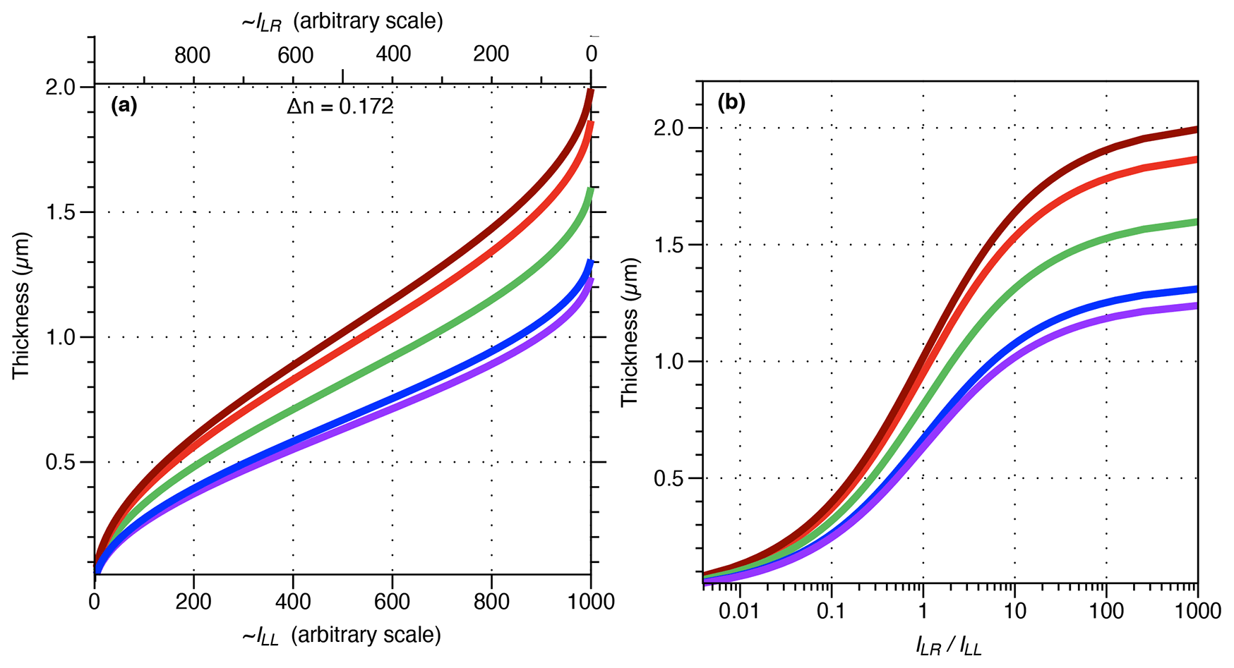
Figure 1 (a) Light intensity (arbitrary scale from min = 0 to max = 1000) going through a left circular polarizer (I_LL) (top scale) or a right circular polarizer (I_LR) (bottom scale) associated with a left circular analyser in relation to the thickness of calcite crystals (birefringence Δn = 0.172), under monochromatic light of wavelengths of 435 nm (indigo curve), 460 nm (blue curve), 561 nm (green curve), 665 nm (red curve) and 700 nm (brown curve). (b) Light intensity ratio (I_LR∕I_LL) under monochromatic light of the same wavelength as in (a) in relation to calcite crystal thickness.

3 Material

The methodology presented here was developed on a Leica DM6000 microscope, with a ×100 objective having a numerical aperture of 1.47 and a condenser lens having a 1.2 numerical aperture (Table 1). Three circular polarizers made by Chroma Technology Corp. are integrated in the microscope. (1) One right circular polarizer is positioned as an analyser. It consists of a linear polarizer oriented at +90^∘ placed below a quarter-wave plate oriented at +45^∘ mounted in a Leica cube and placed in the upper automatic turret of the microscope. This is a convenient place when one wants to automatically remove this analyser to use other filters. Alternatively, the analyser can be placed in its regular position.

Table 1 Microscope parameters and inferred precision of the optics and measurements.

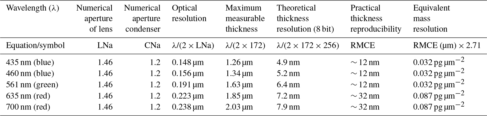
Two polarizers are used alternatively when taking images of the same crystal: (2) a left circular polarizer (LCP) consisting of a quarter-wave plate oriented at +45^∘ followed by a linear polarizer oriented at 0^∘ and (3) a right circular polarizer (RCP) made of a quarter-wave plate oriented at −45^∘ followed by a linear polarizer oriented at 0^∘ .

If possible, the LCP and RCP are placed in the revolving filter chamber of the automated condenser block. For manual use, a quarter-wave plate could be placed under a linear polarizer and rotated manually from +45^∘ (LCP) to −45^∘ (RCP).

One of five monochromatic bandpass filters centred at 435, 460, 560, 655 and 700 nm (AT435/20X, AT460/50M, ZET561/10X, AT655/30M and ET700/50M; all from Chroma Technology Corp.) is positioned in the light trajectory after the light bulb. The 561 nm filter is used in routine work because of its versatility (see below) and it is the one we recommend for general use. The other filters have been used in this study to test the method. On special occasions, we recommend the use of a 700 nm filter to measure calcite particles with thickness ranging between 1.4–1.9 µm and a 460 nm filter for detailed measurements of thin particles in the range of 0.2–0.4 nm.

Two black and white numerical cameras are set up. A SPOT Flex from Diagnostic Instruments, with a charge-coupled device (CCD) image sensor of 2048×2048 pixels that are 7.4 µm large. It is a 14 bit camera (16 383 grey levels in depth). And we use an ORCA-Flash 4.0 V2 from Hamamatsu, with a CMOS image sensor of 2048×2048 pixels that are 6.3 µm wide. It is a 16 bit camera (65 548 grey levels in depth). The tests of this method presented in results have been made with (i) surface sediment retrieved in the southern Pacific and spread onto a slide and (ii) calcium carbonate crystals precipitated onto a slide.

4 Results

To test the quality of the thickness estimations with the BCP method, the same field of view has been studied in different light conditions (brightness, opening and wavelength) and with different cameras. In each condition, the two images I_LL and I_LR are captured and used to compute the thickness d, with Eq. (2). In some cases, in order to illustrate d, an image frame d_i in 8 bit, was computed using the following equation:

$$\begin{array}{}\text{(3)}& d_i=\mathrm{256}{\displaystyle \frac{d}{d_{\max }}},\end{array}$$

where d_max represents the maximum measurable thickness at a given wavelength. It is calculated using the following equation:

$$\begin{array}{}\text{(4)}& d_{\max }={\displaystyle \frac{\mathit{\lambda }}{\mathit{\pi }\mathrm{\Delta }n}}\cdot {\displaystyle \frac{\mathit{\pi }}{\mathrm{2}}}.\end{array}$$

For calcite crystals, d_max ranges between 1.17 µm at 405 nm and 2.03 µm at 700 nm (Table 1).

4.1 Brightness

The same field of view was captured at different exposure times with the SPOT Flex camera. Exposure time is the simplest way to change the brightness of an image. Figure 2 shows that the fields of view captured at short exposure time (e.g. 5 ms) are extremely dark, and conversely those captured at long exposure time (e.g. 320 ms) are light with many saturated areas (maximum grey level (GL) values). Except for those two extreme expositions (i.e. 5 and 320 ms), the GL values, in the resulting images in the bottom row of Fig. 2, are identical. In Fig. 3 the histograms of I_LL, I_LR and d are shown. At 320 ms the images are too light, and many areas are saturated in both I_LL and I_LR and thus have the same GL values. Knowing that the solution of Eq. (2) is 0.81 µm when I_LL=I_LR and λ=561 nm, a spurious density peak appears in the histograms at a thickness of 0.81 µm with an exposure time longer than 320 ms (Fig. 3). In areas where I_LL is saturated but not I_LR, the estimations are shifted toward thicker values, explaining the thicker density pick found at 0.7 µm in the histogram of 320 ms (Fig. 3). The image background, materialized in the histograms by the first peak, is around 0.1 µm for all exposures but is shifted toward higher thickness up to 0.2 µm at 320 ms.

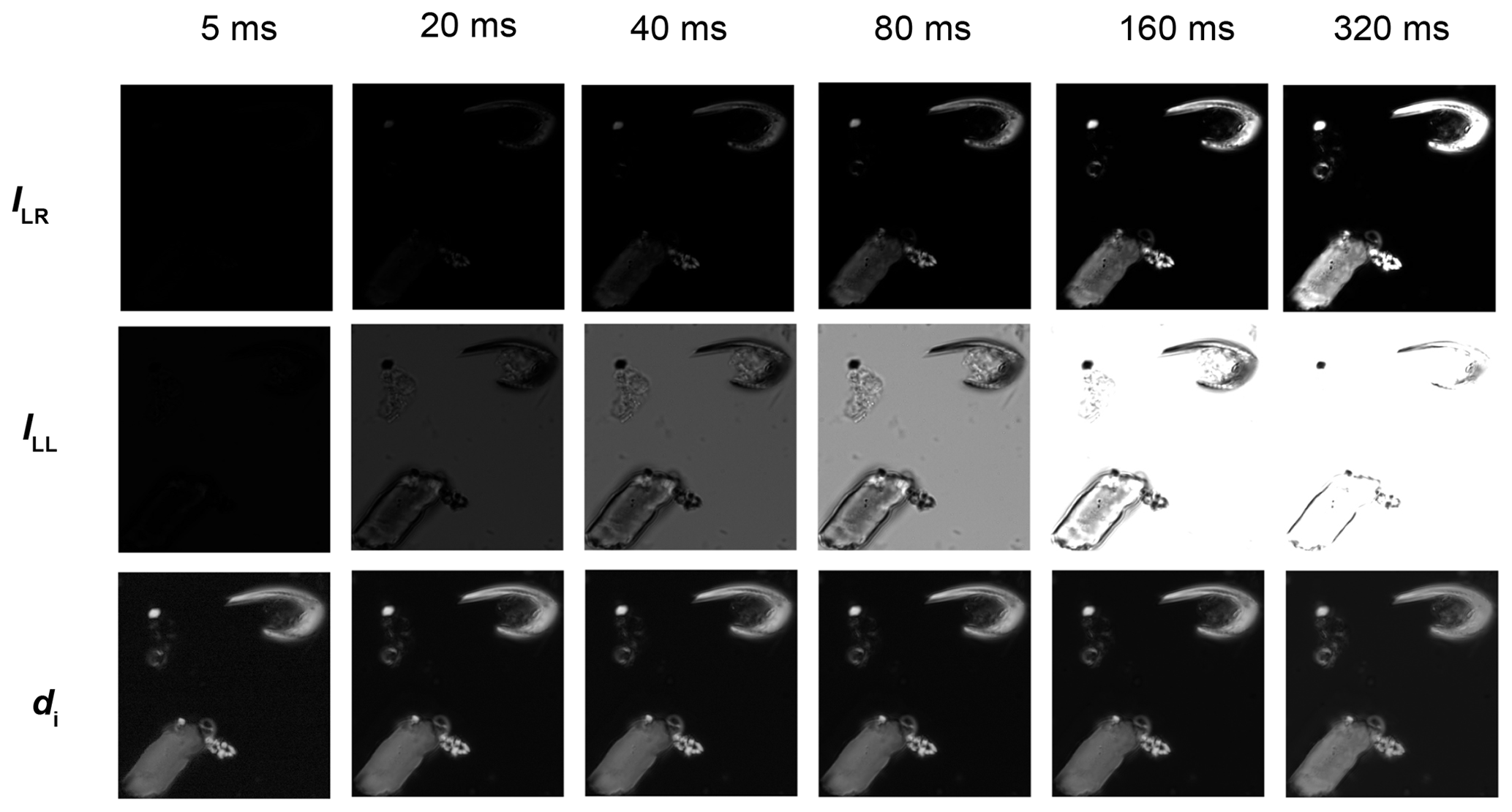
Figure 2 Crops of images captured at different time exposures (in columns; 5, 20, 40, 80, 160, 320 ms) in right circular polarization (first row; I_LR), left circular polarization (second row; I_LL) and resulting thickness using Eqs. (2) and (3) with λ=561 nm (third row; d_i). The resulting thickness images are very similar in the range of time exposure.

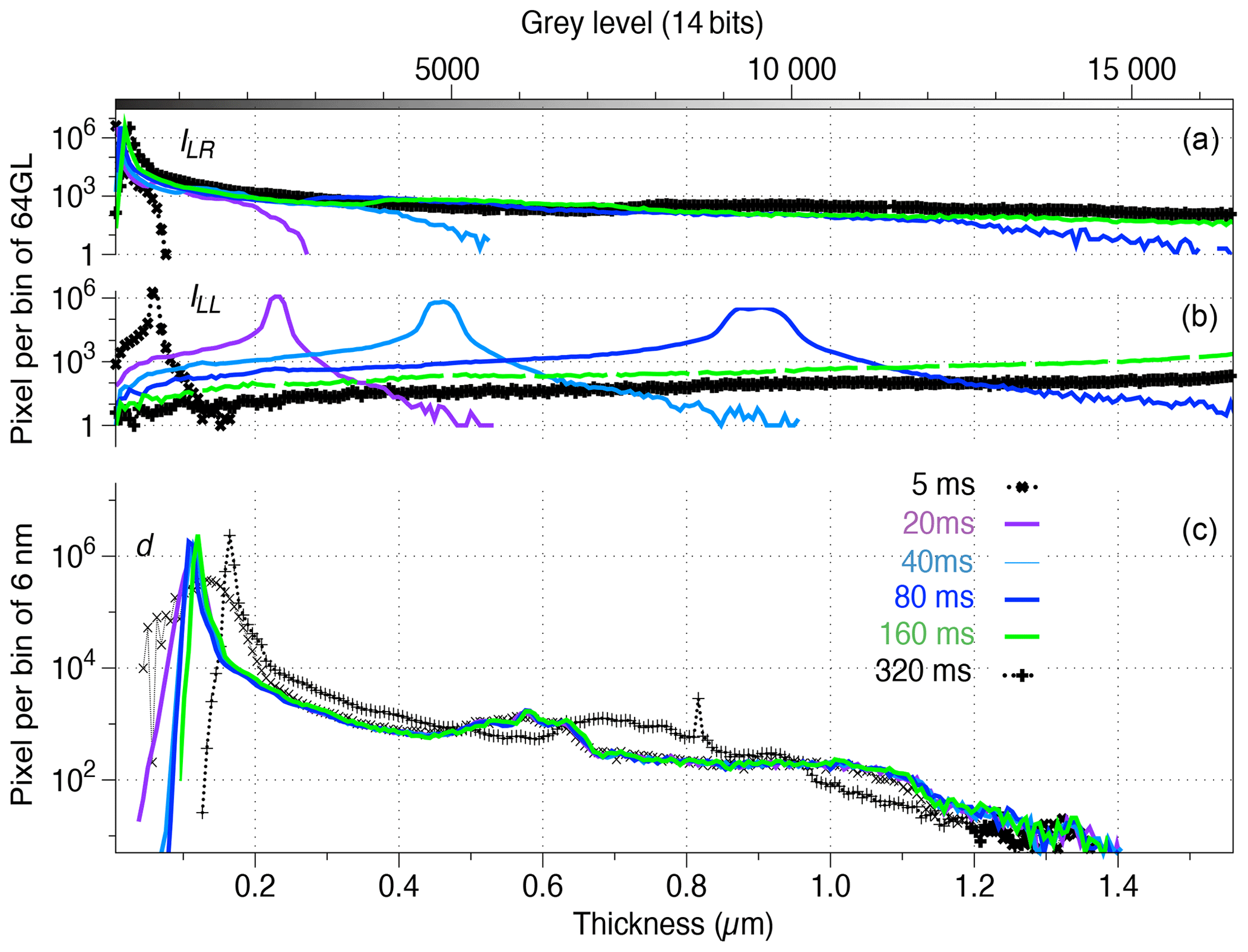
Figure 3 Histograms (bins of 64 grey levels (top) and 6 nm (bottom)) of the same field of view as in Fig. 2, captured with green monochromatic light λ=561 nm in right circular polarization (a), left circular polarization (b) and the resulting thickness using Eq. (2) (c) at different exposure times (black with plus signs: 5 ms, purple: 20 ms, light blue: 40 ms, blue: 80 ms, green: 160 ms, and black with crosses: 320 ms).

At 5 ms, the images are too dark to provide correct estimation of the background level (Fig. 3) which, in turn, increases noise in the results. Therefore, in order to get correct thickness values, it is important to avoid too low or too high brightness. Between those extremes light conditions, the estimates of thicknesses are independent of brightness. To get the maximum depth details, it is suggested to use the maximum light before saturation in I_LL, providing the largest range of grey levels in both images and therefore a larger signal-to-noise ratio in the thickness estimates. In the example given in Fig. 2, this maximum detail would be achieved between 80 and 160 ms.

The optical setting used in this experiment was not able to produce the darkest values (close to 1) and lightest value (equivalent to 255 in 8 bit). The reason why those extreme values are not reached is largely due to the imperfections of the circular polarizers that are composed of two layers. Those imperfections are amplified at the extremes of the light ranges because of the sigmoid shape of the thickness function (Fig. 1). In practice, the ratio I_LR∕I_LL is reached in the flattest part of the sigmoids (Fig. 1b), for example between 0.10 and 1.41 µm with a 561 nm light wavelength. As a consequence, the thickness measured in an empty part of the field of view was 0.10 µm at 561 nm when it should be 0. Also, the maximum measurable thickness is lower than the maximum theoretical thickness: using a wavelength of 561 nm, we obtain a maximum of 1.45 µm of thickness instead of 1.62 µm (Fig. 3).

4.2 Aperture

The illumination tuning of the microscope is also important. The range of measurable thickness is largest when the condenser is focused and centred following the Köhler illumination (Köhler, 1894). The more closed the field diaphragm, the wider the range of measurable thickness (Fig. 4). Hence, both diaphragms (i.e. field and aperture) should be closed at their maximum in order to maximize the range of measurable thickness.

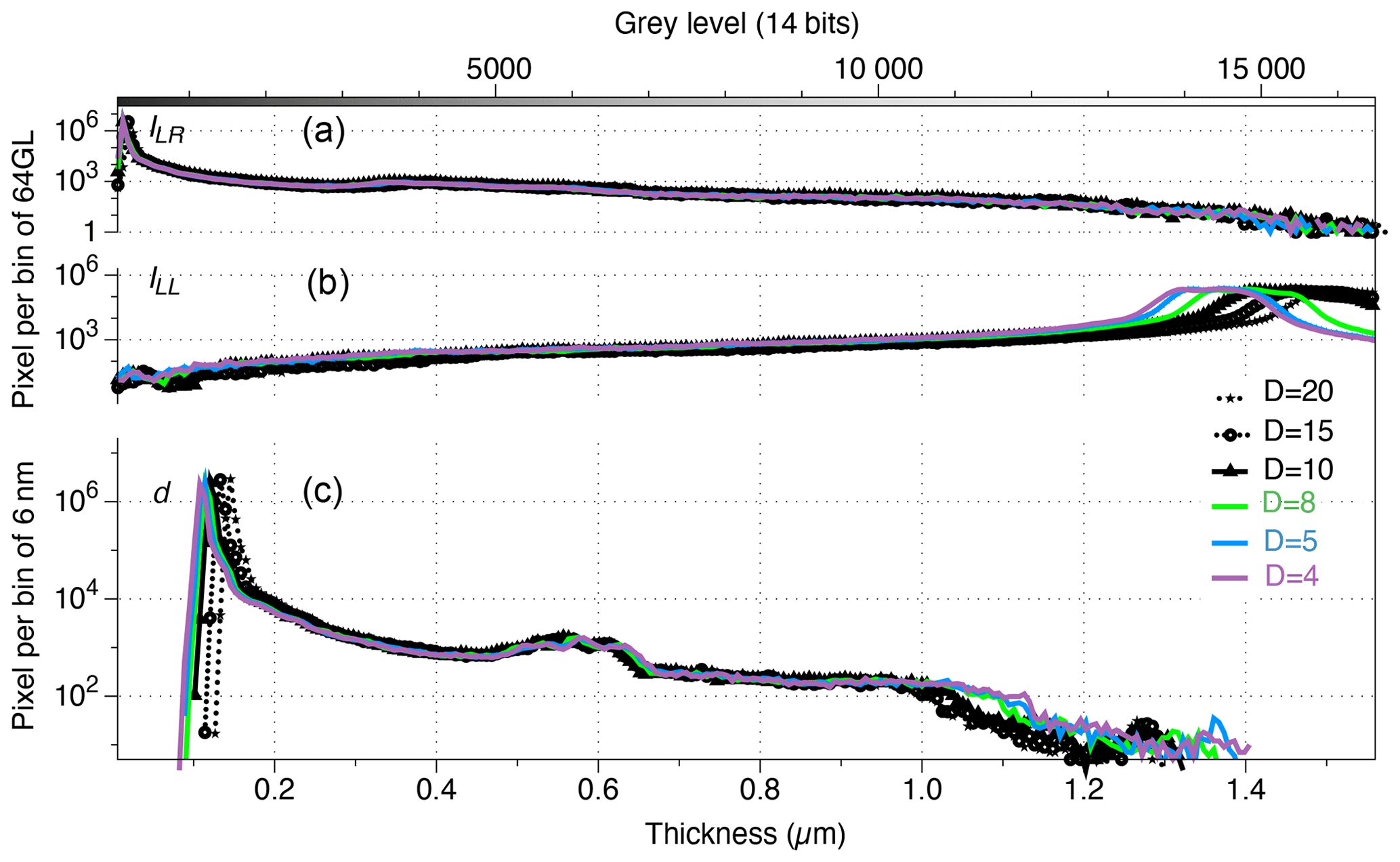
Figure 4 Histograms (bins of 64 grey levels (top) and 6 nm (bottom)) of the same field of view as in Fig. 2, captured with green monochromatic light λ=561 nm in right circular polarization (a), left circular polarization (b) and the resulting thickness using Eq. (2) (c) at different openings (Leica DM6000B scale ranging from 1 (closed) to 20 (open)) of the field diaphragm (black with stars: 20; black with circles: 15; black with squares: 10; green: 8; blue: 5; and purple: 4).

4.3 Camera type

The two tested camera types (CMOS vs CCD; 14 bit vs. 16 bit; different brand) produced the same results. The same view field was captured with two different camera types without measurable difference between the two resulting thickness images (Fig. 5).

Figure 5 (a) Thickness along a transect (yellow line in the inset) measured with the SPOT flex (red line with crosses) and the ORCA-Flash cameras (blue line with plus signs). (b) Relation between I_LL (red), I_LR (blue) and thickness (black) measurements made by the two cameras along the same transect.

The theoretical maximum measurable thickness (d_cmax) depends on the number of grey levels (nGL) achieved by the camera:

$$\begin{array}{}\text{(5)}& d_{\mathrm{cmax}}={\displaystyle \frac{\mathit{\lambda }}{\mathit{\pi }\mathrm{\Delta }n}}\arctan \left(\sqrt{{\displaystyle \frac{n\mathrm{GL}}{\mathrm{1}}}}\right).\end{array}$$

At λ=561 nm, d_cmax is 1.565 µm with an 8 bit camera, 1.622 µm with a 14 bit camera and 1.626 µm with a 16 bit camera. These d_cmax values are far above the maximum measurable thickness of 1.45 µm described in Sect. 5.1. However, the low depth resolution of an 8 bit camera should further limit the range of measurable thickness, although this was not tested here. Hence, both 14 and 16 bit can be used but we do not recommend using 8 bit camera.

4.4 Accuracy and precision

It is extremely difficult to estimate the measurement error in the present case because there is no standard material for thickness comparison in the range of a few nanometres. The thickness of the wedge used to estimate the accuracy in González-Lemos et al. (2018) is measured at 250 nm intervals, which is not enough in our case. Also, its measurements are based on a birefringence principle that is not strictly independent from our methodology. However, González-Lemos et al. (2018) clearly validate the accuracy of birefringence method at 250 nm. The measurement of coccoliths made by coherent X-ray diffraction (CXDI) at ESRF (Beuvier et al., 2019) requires the use of silicon nitride (Si₃N₄) TEM windows influencing birefringence. Hence, those coccoliths cannot be used later as a standard. However, in this study, coccolith mass and size measurements from the same culture using both birefringence and CXDI provide a comparison on statistically similar results. The validity of the birefringence method is also demonstrated, although without giving a value to the accuracy. The use of cylindric rods such as rhabdoliths (Beaufort et al., 2014; Fuertes et al., 2014) is limited by the precision of the microscope used to produce the measurement of their diameter, around 0.2 µm in our microscope, and likely due to issues with natural variations in rhabdoliths (parts of which may be hollow). The BCP method does not use any calibration; it is therefore theoretically absolute. It is accurate in the range given by the inflection points in Fig. 1.

We determine the precision of the BCP method at the five different wavelengths by using the two cameras on the same 7.74 µm transect of a Pontosphaera japonica (Fig. 6), producing 10 series of measurements. At the difference with Fig. 5, and to produce feasible “user noise”, we have slightly shifted the focus and use different wavelengths. The root-mean-square error (RMSE) between two series is used to determine the precision of the method. The RMSE ranges between 14 and 47 nm. The largest RMSE values result from the largest focus differences and/or red colours (635 and 700 nm). The best results were obtained at 561 and 435 nm with similar focus. When one series of measurements was compared to the average of all the other series, the RMSE = 32 nm. When it is limited to 435 to 561 nm, the RMSE = 12 nm. As we explain in detail in the next section, longer wavelengths in red lower the precision. This is an order of magnitude smaller than the spatial optical resolution which ranges between 150 and 240 nm in the present microscopic setting at the five different wavelengths. The precision of the BCP method is expected to be smaller in many cases. For example, the RMSE in the transect of Fig. 5 is 5 nm. The difference of RMSE between Figs. 5 and 6 is essentially related to the focus that was well reproduced in Fig. 5. The measurable masses of P. japonica in Fig. 6 range from 65.3 to 69.9 pg with a standard deviation of 1.28 pg (N=10) and depend again on the wavelength and the focus.

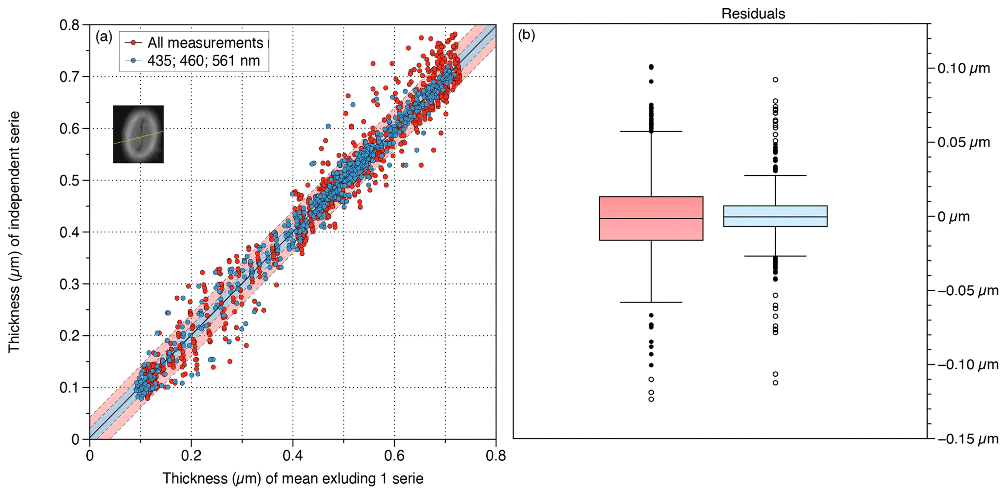
Figure 6 Precision of measurements made on the same 7.74 µm transect (yellow line in the inset) across a Pontosphaera japonica (inset) with two cameras and at five or three wavelengths, producing respectively 10 or six series of 129 points. Red: all wavelengths (r²=0.996; RMSE = 0.032 µm); blue: 435, 460 and 561 nm (r²=0.994; RMSE = 0.012 µm). (a) Relation between measure of a thickness series compared with the average of all the others. The average thickness of nine (or five) series along a transect and the thickness in the independent (not included in the average) series. The coloured area represents the 80 % prediction bounds. (b) Whisker plots of the residual; bars represent the interquartile range, and the box represents the range between the first and third quartiles. Standard deviation = 0.032 (left in red) and = 0.019 (right in blue).

4.5 Wavelength and range of measurable thickness

The comparisons of the same transects captured at different wavelengths along an image frame containing thick CaCO₃ particles emphasize the advantages and limits of each light wavelength. The range of thickness measurable at a given wavelength is presented in Fig. 7. In the transects, a plateau is reached at the maximum practical thickness (MPT); when the particle thickness is about 0.5 µm above the MPT, the thickness values decrease. It is not entirely clear why MPT is about 84 % lower than the maximum measurable thickness (d_max). This difference has been described earlier (Bollmann, 2014). This discrepancy could be resulting from the quality of circular polarizers used. The circular polarizers are made with polaroid filters that are not perfect and are composed of two filters – a quarter-wave plate and a polarizer – creating some imperfections. As an example, linear polarizers exhibit a generally larger range of grey levels with darker background than circular polarizers.

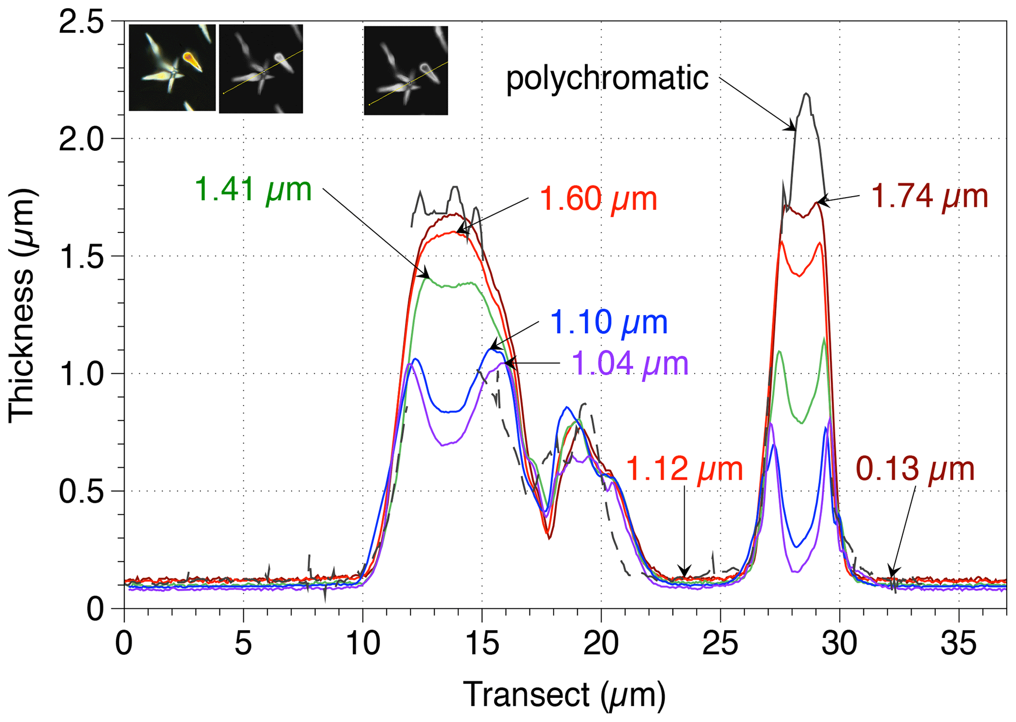
Figure 7 Thickness measurements made along two transects (T.1 in red and T.2 in white lines in the left inset) of CaCO₃ crystals at five wavelengths (brown lines: 700 nm; red lines: 635 nm; green lines: 561 nm; blue lines: 460 nm; indigo lines: 435 nm) and with polychromatic light grabbed by a colour camera (black lines; using the hue values transfer function for thickness from Beaufort et al., 2014 – this latter method allows measurement up to a thickness of 4.5 µm after a complex calibration; dotted black line is the thickness measured with the logit function in Beaufort et al., 2014, that transfers GL in thickness values: note that for this image the white balance is not perfect). The three insets represent the images taken with a colour camera (SPOT Flex) (left), a black and white camera (SPOT Flex) at 700 nm (centre), and the same camera at 435 nm (right). The maximum and minimum measurements for each wavelength are indicated with an arrow.

For the study coccoliths thicker than 1 µm like those of the Eocene, we recommend using a light with long wavelengths (e.g. red at 700 nm). On the contrary, for the study of thin coccoliths such as the most extant and Pleistocene species, we recommend using shorter wavelengths (e.g. green or blue). Short wavelengths reached a MPT at a lower thickness but offer higher precision in the measurement of the thickness and higher optical resolution, permitting higher precision in the measurement of the area. Plate 1a shows an Emiliania huxleyi coccolith, in which the slits, which are present in the distal shield, appear only in blue light. This illustrates an extreme case, for which the low wavelength has to be used to get a most precise thickness and mass measurements. The distal shield of E. huxleyi is constructed with thin – ∼ 100 nm – elements that do not touch each other (Plate 1a). The detection of those elements above the background is extremely difficult using wavelengths at 700 nm but is possible using wavelengths at 435 nm. As a consequence, mass measurements are underestimated at 700 nm because the distal shield is not completely detected and producing a total area smaller than it is really (Table 2). Finally, this new method cannot give accurate results for calcareous nannofossils with a thickness above 1.7 µm like Cretaceous Nannoconus species. For such material, we recommend being critical with results close to MPT and using a colour camera (Beaufort et al., 2014; González-Lemos et al., 2018) as in Fig. 7, although less precise than the BCP method related to colour calibration issues (González-Lemos et al., 2018).

Table 2 Measurements at different wavelengths of the coccoliths of Emiliania huxleyi presented in Plate 1.

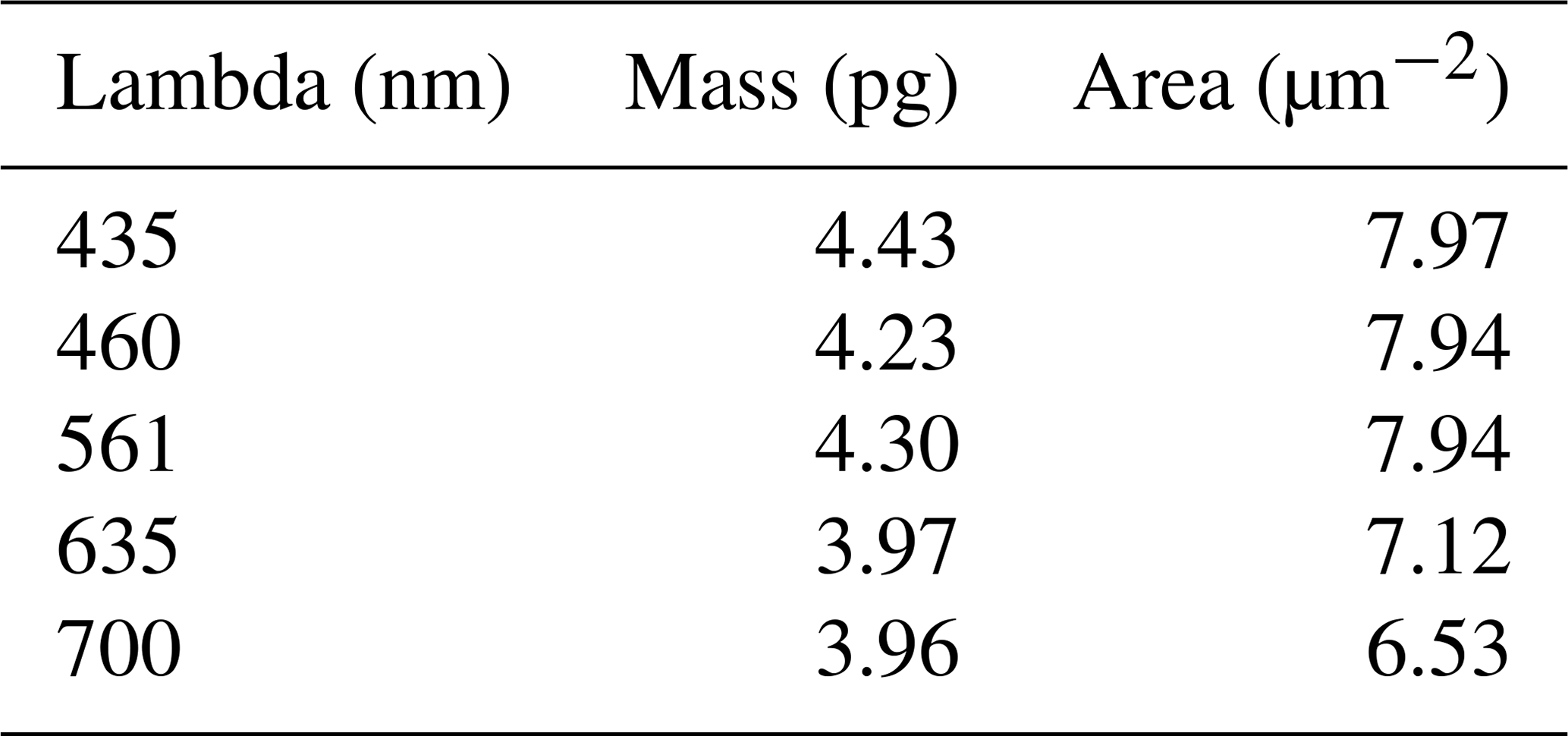
Table 3 Average morphology results of population of Emiliania huxleyi coccoliths measured on three different supports.

5 Protocol

1. The microscope setting is as follows: Köhler illumination done, diaphragms as closed as possible, circular polarizers (with a rotating quarter-wave plate or two circular polarizers: one left oriented and one right oriented), circular analyser, monochromatic filter.

2. Grab one image of a field of view with the circular polarizer oriented to the left (image ILL).

3. Grab one image of the same field of view with the circular polarizer oriented to the right (image ILR).

4. Compute the image d_i with Eq. (3): $d_i=\mathrm{256}\frac{d}{d_{\max }}$, with d from Eq. (2): $d=\frac{\mathit{\lambda }}{\mathit{\pi }\mathrm{\Delta }n}\arctan \left(\sqrt{\frac{I_{\mathrm{LR}}}{I_{\mathrm{LL}}}}\right)$, and d_max from Eq. (4).

   $$d_{\max }={\displaystyle \frac{\mathit{\lambda }}{\mathit{\pi }\mathrm{\Delta }n}}\cdot {\displaystyle \frac{\mathit{\pi }}{\mathrm{2}}}{d}_i$$

   can be simplified into

   $$\begin{array}{}\text{(6)}& d_i=\mathrm{163}\arctan \left(\sqrt{{\displaystyle \frac{I_{\mathrm{LR}}}{I_{\mathrm{LL}}}}}\right).\end{array}$$

   An example of a Python routine that calculates the output image d_i is given here.

   # Import.Lib.
   import sys
   from PIL import Image
   import math
   from math import pi
   # open Image file
   img_ILL = Image.open("/Path/image
                         ILL.tif")
   img_ILR = Image.open("/Path/image
                         ILR.tif")
   # Create output image
   img_d = Image.new(img_ILL.mode,
   img_ILL.size)
   # Get image size
   column,line = img_ILL.size
   # Compute d for every pixel
   for i in range(line):
      for j in range(column):
       ILL_val = img_ILL.getpixel((j,i))
                 + 1
       ILR_val = img_ILR.getpixel((j,i))
       # Compute thickness values
       d = 163 * math.atan(math.sqrt
                 (ILR_val / ILL_val))
       # Output image
       img_d.putpixel((j,i), (int(d),))
   # Show thickness image
   img_d.show

5. The point measurement is as follows: d_i is an image that is scaled in grey levels and not in micrometres. In order to get the thickness at one point (pixel) of an image, get the grey level value, GL, at this position.

   From Eq. (3) we obtain

   $$\begin{array}{}\text{(7)}& d={\displaystyle \frac{d_i{d}_{\max }}{\mathrm{256}}}.\end{array}$$

   d_max is given in Eq. (4). For example for a calcite crystal (Δn=0.172) and using a green monochromatic light of λ= 0.561 µm, d_max is 1.63 µm. In that case GL must be divided by 160 in order to get the thickness at that point.

   When one wants to measure a particle (instead of a point) it may continue as follows.

6. Threshold. One must withdraw the background of the image without changing the GL values of the particle. An easy way to do that is explained in the following ImageJ plugin. In this example the maximum background GL value is 19.

   run("Duplicate...", " ");
   setThreshold(19, 255);
   setOption("BlackBackground", false);
   run("Convert to Mask");
   run("Divide...", "value=255.000");
   imageCalculator("Multiply create",
        "image.tif","image-copy.tif");
   selectWindow("Result of image.tif");

7. Average thickness ($\stackrel{\mathrm{‾}}{d}$). To measure the lightness of the particle, select the region of interest (ROI) containing an isolated particle. Measure the mean GL value of the ROI. Use Eq. (6) to calculate the average thickness in micrometres of the particle.

8. Mass of the particle. Mass $=\stackrel{\mathrm{‾}}{d}a\mathit{\rho }$, where a is the area in micrometres and ρ is density of calcite in picogrammes per cubic micrometre (= 2.71). The mass is in picogrammes.

Plate 1 Images of a coccolith of Emiliania huxleyi captured at wavelengths 435 (a) and 700 nm (b). White bars are 1 µm long. Brightness has been adapted to enhance the contrast between background and elements from the distal shield.

6 Limits of protocol

1. Thickness. As it was said earlier, this method is not applicable for particles thicker than the practical d_max, which is 2 µm using red light. This is not a strong limitation for coccoliths since most of them are not thicker than 1.5 µm. In quaternary sediments, where the coccoliths are as a majority <1.2 µm thick, we prefer to use a blue colour that gives the most precise results. When working with Miocene–Pliocene sediments, a green light is recommended because of large Reticulofenestra. In Paleogene sediments it may be interesting to work with a red light.

2. v units. The BCP method is perfect for calcite crystals having their optical axis oriented perpendicular to the light trajectory. During the crystallization of coccoliths, many crystals have their optical axis radially oriented, the so-called r units described by Young et al. (1992). Those coccoliths (e.g Noelaerhabdaceae) are well measured by any polarization method including BCP. In some species, the coccoliths have two types of crystals: those with the optical axis oriented radially (r units), and those with a vertical optical axis (v units) (Young et al., 1992). The thickness of crystals having a v unit cannot be measured by birefringence methods. In some genera such as Pontosphaera it does not impact significantly because the proportion of v unit is limited. In some genera such as Coccolithus, a larger proportion of the coccoliths are composed of v units (the distal shield), and it is possible to use a correction factor as proposed by Cubillos et al. (2012). For coccoliths composed exclusively of v units such as the discoasters, BCP and other birefringent methods are not applicable.

3. Sample preparation. Most of the preparation methods used in the study of fossil samples use glass as a support, whereas some methods use membrane with a small porosity (e.g. 0.45 µm) in order to retain the coccolith on it (see Giraudeau and Beaufort, 2007, for a review). Such methods are classically used when studying living coccolithophore assemblages. The collected seawater is filtered on a membrane that is subsequently mounted between slide and coverslips with a mounting media that is sufficiently liquid to make the membrane almost transparent. Three types of membranes are used: acetate cellulose, nitrate cellulose and polycarbonate. The membranes are not completely transparent and this affects the measure of thickness. To quantify this effect, we mounted the same sample on glass only (GO), with membrane on acetate cellulose (AC) and with polycarbonate membrane (PC). The background level measured in blue (560 nm) was 14, 16 and 19 GL with GO, AC and PC respectively. The “opacity” of the membranes add two GLs for AC and five GLs for PC, corresponding respectively to the thickness of 11 and 26 nm or to mass per square metre of 0.03 and 0.07 pg. These values are in the same order of precision as expected with the BCP method. Because it is not possible to measure the same object on the three types of support, we measure the average mass and thickness of coccoliths from a large population belonging to the same species (E. huxleyi) in the same sample replicates (MD97-2125; 5 cm). We did not find any significant difference between the population measured on the different supports (Table 3). There is no apparent limitation to measure calcite thickness on membranes of that type. The small holes in the polycarbonate membranes are not filled by the medium. They appear opaque when observed in the microscope in both natural and circular polarized light (right and left). These holes can be seen by transparency through calcite particles. In the BCP image projections, the holes do not appear prominently, and they are half darker and half lighter than the background, inducing a small but significant noise in the resulting thickness. Although this effect is not large, the use of this membrane is not recommended when it is possible to use acetate cellulose membranes.

7 Conclusions

The alternative use of left and right circular polarization permits the measurement of the thickness of calcite crystals in a universal manner without precise calibration of light. The BCP method has a great advantage over previous methods for which it is difficult to maintain stable light (i) in time (i.e. bulb ageing, condenser vertical position) and (ii) in space since the field of view may not be uniformly illuminated (i.e. low-quality lens, uncentred condenser). In all these situations, the previously published linear or circular polarizer methods will provide different thickness measurements whereas the BCP method described here will provide the same values. The choice of the wavelength of the light used for the measurements is specific to a targeted thickness. Thicker crystals will require longer wavelengths. Shorter wavelengths are recommended for precise measurement of thin crystals. In practice, upper and lower limits of measurements depend on the quality of polarizers and on the tuning of the microscope (Kohler illumination and narrow diaphragms). With our microscope, the practical range of measurements is 84 % of the theoretical range. For example, at 561 nm, the lower measurable thickness is 0.10 µm and the largest is 1.45 µm when theoretically the range should be 0 to 1.61 µm. It could be interesting to test whether other types of circular polarizers such as mineral ones could provide larger practical ranges. The precision of the thickness measurements are an order of magnitude smaller – 0.012 to 0.030 µm – than measurements of the length related to the resolution of an optical microscope that is approximatively 0.20 µm using natural light.