The impact of the South-East Madagascar Bloom on the oceanic CO₂ sink

We described new sea surface CO₂ observations in the south-western Indian Ocean obtained in January 2020 when a strong bloom event occurred south-east of Madagascar and extended eastward in the oligotrophic Indian Ocean subtropical domain. Compared to previous years (1991–2019) we observed very low fCO₂ and dissolved inorganic carbon concentrations (C_T) in austral summer 2020, indicative of a biologically driven process. In the bloom, the anomaly of fCO₂ and C_T reached respectively −33 µatm and −42 µmol kg⁻¹, whereas no change is observed for alkalinity (A_T). In January 2020 we estimated a local maximum of air–sea CO₂ flux at 27^∘ S of −6.9 mmol m⁻² d⁻¹ (ocean sink) and −4.3 mmol m⁻² d⁻¹ when averaging the flux in the band 26–30^∘ S. In the domain 25–30^∘ S, 50–60^∘ E we estimated that the bloom led to a regional carbon uptake of about −1 TgC per month in January 2020, whereas this region was previously recognized as an ocean CO₂ source or near equilibrium during this season. Using a neural network approach that reconstructs the monthly fCO₂ fields, we estimated that when the bloom was at peak in December 2019 the CO₂ sink reached −3.1 (±1.0) mmol m⁻² d⁻¹ in the band 25–30^∘ S; i.e. the model captured the impact of the bloom. Integrated in the domain restricted to 25–30^∘ S, 50–60^∘ E, the region was a CO₂ sink in December 2019 of −0.8 TgC per month compared to a CO₂ source of +0.12 (±0.10) TgC per month in December when averaged over the period 1996–2018. Consequently in 2019 this region was a stronger CO₂ annual sink of −8.8 TgC yr⁻¹ compared to −7.0 (±0.5) TgC yr⁻¹ averaged over 1996–2018. In austral summer 2019–2020, the bloom was likely controlled by a relatively deep mixed-layer depth during the preceding winter (July–September 2019) that would supply macro- and/or micro-nutrients such as iron to the surface layer to promote the bloom that started in November 2019 in two large rings in the Madagascar Basin. Based on measurements in January 2020, we observed relatively high N₂ fixation rates (up to 18 nmol N L⁻¹ d⁻¹), suggesting that diazotrophs could play a role in the bloom in the nutrient-depleted waters. The bloom event in austral summer 2020, along with the new carbonate system observations, represents a benchmark case for complex biogeochemical model sensitivity studies (including the N₂ fixation process and iron supplies) for a better understanding of the origin and termination of this still “mysterious” sporadic bloom and its impact on ocean carbon uptake in the future.

1 Introduction

In the south-western subtropical Indian Ocean a phytoplankton bloom, called the South-East Madagascar Bloom (SEMB), occurs sporadically during austral summer (December–March, Fig. 1). Based on the first years of SeaWiFS (Sea-Viewing Wide Field-of-View Sensor) satellite chlorophyll a (Chl a) observations in 1997–2001, the SEMB was first recognized by Longhurst (2001) as the largest bloom in the subtropics, extending over 3000 km × 1500 km in the Madagascar Basin. When the SEMB is well developed like in February–March 1999 (Longhurst, 2001), monthly mean Chl a concentrations are higher than 0.5 mg m⁻³ within the bloom, contrasting with the low Chl a in the surrounding oligotrophic waters (<0.05 mg m⁻³). For reasons still not fully understood, this bloom occurred in specific years (1997, 1999 and 2000) but was absent or moderate during a strong El Niño–Southern Oscillation (ENSO) event in 1998. Following the first study by Longhurst (2001), the frequency, extension, levels of Chl a concentration, and processes that would control the SEMB and its variability have been investigated in several studies (Srokosz et al., 2004; Uz, 2007; Wilson and Qiu, 2008; Poulton et al., 2009; Raj et al., 2010; Huhn et al., 2012; Srokosz and Quartly, 2013). Most of these studies were based on Chl a derived from remote sensing and altimetry. They all concluded the need for in situ observations to understand the initiation, extent and termination of the SEMB. To our knowledge in situ biogeochemical observations (Chl a, phytoplanktonic species and nutrients) within the SEMB region were only obtained during MadEx (Madagascar Experiment) in February 2005 (Poulton et al., 2009; Srokosz and Quartly, 2013), a year when the bloom was not well developed (e.g. Uz, 2007; Wilson and Qiu, 2008). The MadEx cruise was conducted above the Madagascar Ridge and west of 51^∘ E in the Madagascar Basin. However, the eastward extension of the SEMB occasionally reached the central oligotrophic Indian Ocean subtropics (longitude of 70^∘ E, Fig. 1b) where the bloom is transported and apparently bounded by the South Indian Counter Current (SICC) around 25^∘ S (Siedler et al., 2006; Palastanga et al., 2007; Huhn et al., 2012; Menezes et al., 2014). A recent analysis of the East Madagascar Current (EMC) and its retroflection near the southern tip of Madagascar also suggests that a complex dynamic sometimes promotes the SEMB (Ramanantsoa et al., 2021). Modelling studies also suggested an eastward propagation of the SEMB through advection or eddy transport originating from the south-eastern coast of Madagascar (Lévy et al., 2007; Srokosz et al., 2015; Dilmahamod et al., 2020), but a precise explanation of the internal (e.g. local upwelling, Ekman pumping and mesoscale dynamics) or external processes (e.g. iron from rivers, coastal zones or sediments) at the origin of this “mysterious” bloom is still missing.

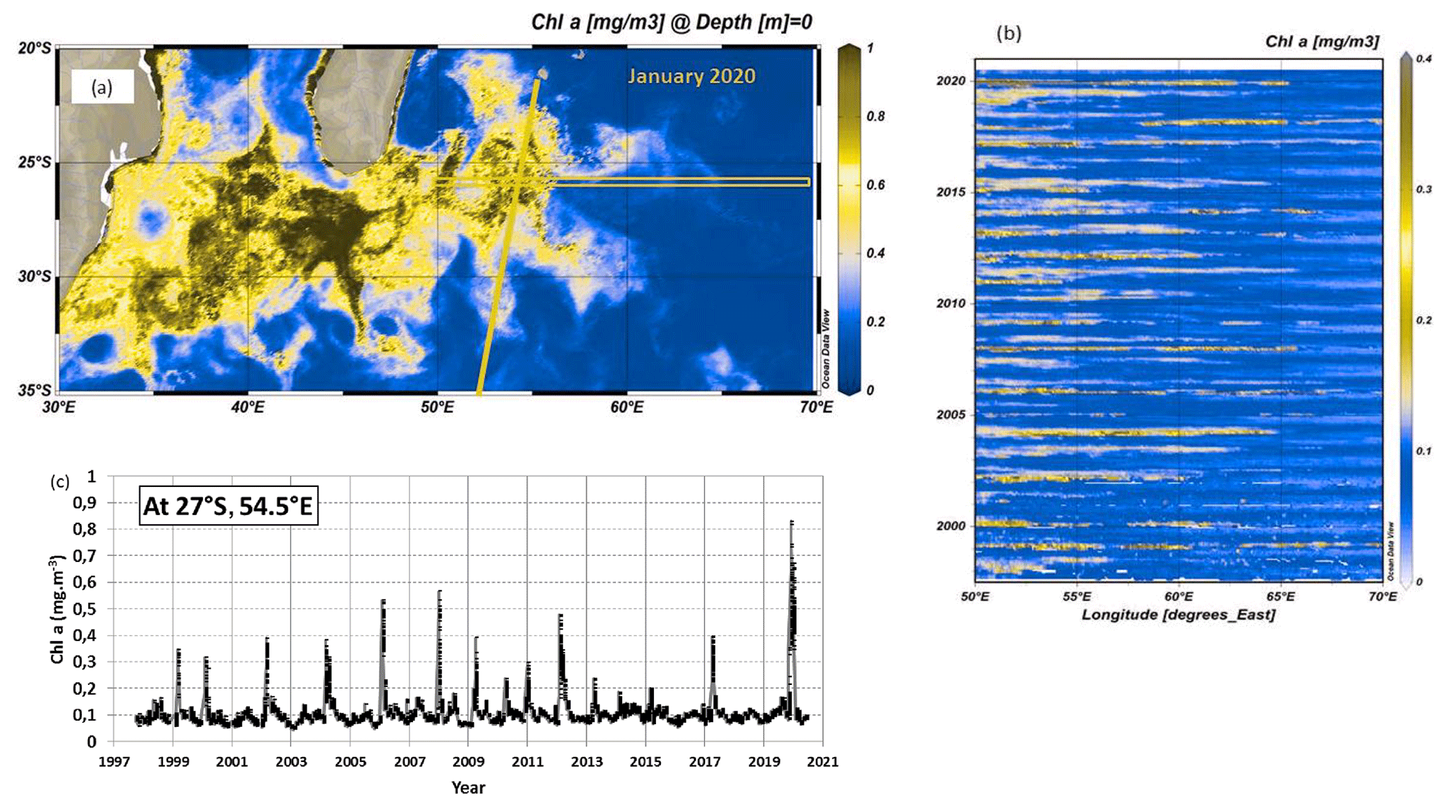
Figure 1 (a) Map of monthly surface Chl a (mg m⁻³) in the south-western Indian Ocean in January 2020 derived from MODIS data (4 km × 4 km resolution), highlighting the bloom south and south-east of Madagascar. (b) Hovmoller time series (time and longitude) of Chl a (mg m⁻³) around 26.5^∘ S along 50–70^∘ E (orange box in a). (c) Time series of monthly Chl a (mg m⁻³) at 27^∘ S, 54.5^∘ E (only when the valid number of pixels is greater than five for each point). The orange line on the map identifies the track of the OISO-30 cruise. The figures highlight the high Chl a concentration in austral summer 2020. Panels (a) and (b) produced with ODV (Ocean Data View; Schlitzer, 2013) from data downloaded from https://resources.marine.copernicus.eu/ (OCEANCOLOUR_GLO_CHL_L4_REP_OBSERVATIONS_009_093, last access: 10 April 2021).

The above studies have been recently synthesized by Dilmahamod et al. (2019), who also proposed an index to determine the level of the SEMB (strong, moderate or absent) based on the difference in Chl a concentrations between the western and eastern regions centred respectively around 55 and 80^∘ E at 24–28^∘ S. Quoting Dilmahamod et al. (2019), “The South-East Madagascar Bloom is one of the largest blooms in the world. It can play a major role in the fishing industry, as well as capturing carbon dioxide from the atmosphere.” Although numerous cruises measuring sea surface CO₂ fugacity (fCO₂) have been conducted since the 1990s in the south-western Indian Ocean region (Poisson et al., 1993; Metzl et al., 1995; Sabine et al., 2000; Metzl, 2009), the impact of the SEMB on air–sea CO₂ fluxes was not previously investigated. This is probably because the bloom was not strong enough at the time of the cruises to identify large fCO₂ anomalies in this region. Therefore, the temporal (seasonal and/or inter-annual) fCO₂ variability in the western and subtropical Indian Ocean is generally interpreted by thermodynamics as the main control, with biological activity and mixing processes being secondary driving processes in this oligotrophic region (Louanchi et al., 1996; Metzl et al., 1998; Sabine et al., 2000; Takahashi et al., 2002). On the other hand, all climatologies based on observations suggest rather homogeneous sea surface fCO₂ or dissolved inorganic carbon (C_T) fields in this region (Takahashi et al., 2002, 2009, 2014; Lee et al., 2000; Sabine et al., 2000; Bates et al., 2006; Lauvset et al., 2016; Zeng et al., 2017; Broullón et al., 2020; Keppler et al., 2020; Fay et al., 2021; Gregor and Gruber, 2021). This suggests that, although the SEMB and its extent have been regularly observed since 1997, it seems to have a small effect on fCO₂ or C_T spatial variations. However, in austral summer 2019/20, the SEMB was particularly pronounced, reaching monthly mean Chl a concentrations up to 2.5 mg m⁻³ at the peak of the bloom in December 2019. It was clearly much stronger than previously observed, at least since 1997 (Fig. 1), and reflected in fCO₂ observations in this region (Fig. 2).

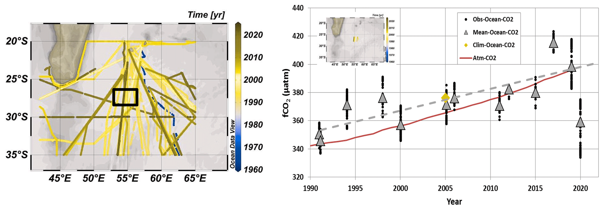
Figure 2 On the left are shown tracks of cruises with sea surface fCO₂ data available in the south-western Indian Ocean in the SOCAT data product (Surface Ocean CO₂ Atlas; SOCAT v2021, Bakker et al., 2016, 2021). On the right is shown a time series of fCO₂ data (black dots) and mean fCO₂ for each period (grey triangles) at 27–28^∘ S, 55^∘ E (black square in the map and insert on the right) for the months of January and February (data available from 1991 to 2020 for austral summer). The red curve is the atmospheric fCO₂. Although over 1991–2019 the ocean fCO₂ increased by +1.55 (±0.40) µatm yr⁻¹ (dashed grey line) due to anthropogenic CO₂ uptake, the fCO₂ recorded in January 2020 in the bloom were low compared to previous years with some values below 340 µatm, i.e. lower than in 1991. The January–February-averaged fCO₂ in the same region derived from the 2005 climatology of Takahashi et al. (2014) is also plotted (orange diamond). Map on the left produced with ODV (Schlitzer, 2013).

In this analysis, we describe new oceanic carbonate system observations in surface waters obtained in January 2020 associated with this very strong SEMB event and compare these observations with climatological values and previous fCO₂ data when the SEMB was not well developed. We also evaluate the impact of the bloom on air–sea CO₂ fluxes based on both observations and reconstructed monthly fCO₂ fields in the south-western Indian Ocean.

2 Data collection

As part of the long-term OISO project (Océan Indien Service d'Observations), the OISO-30 cruise was conducted in austral summer 2020 (from 2 January to 6 February 2020) onboard the RV Marion Dufresne in the southern Indian Ocean (part of the track shown in Fig. 1). During the cruise, underway continuous surface measurements were obtained for temperature (SST), salinity (SSS), the fugacity of CO₂ (fCO₂), the total alkalinity (A_T) and the total dissolved inorganic carbon (C_T). Analytical methods followed the protocol used since 1998 and previously described for other OISO cruises (e.g. Metzl et al., 2006; Metzl, 2009; Lo Monaco et al., 2021). Sea surface temperature and salinity were measured continuously using an SBE45 thermosalinograph. Salinity data were controlled by regular sampling and conductivity measurements (Guildline Autosal 8400B and using the IAPSO – International Association for the Physical Sciences of the Oceans – standard or OSIL – Ocean Scientific International). The SST and SSS data were also checked against CTD (conductivity–temperature–depth) surface records when available. Accuracies of SST and SSS are respectively 0.005 ^∘C and 0.01. Total alkalinity (A_T) and total dissolved inorganic carbon (C_T) were measured continuously in surface water (three to four samples per hour) using a potentiometric titration method (Edmond, 1970) in a closed cell. For calibration, we used the certified reference materials (CRMs, batch no. 173) provided by Andrew Dickson (SIO – Scripps Institution of Oceanography, University of California). Replicate measurements were occasionally performed at the same location. At 30^∘ S, 54^∘ E for four replicates the mean A_T and C_T concentrations were respectively 2328.6 (±0.7) and 1998.2 (±1.6) µmol kg⁻¹. At 35^∘ S, 53.5^∘ E for six replicates the mean A_T and C_T were 2340.5 (±0.6) and 2060.6 (±1.1) µmol kg⁻¹. Overall, we estimated the accuracy for both A_T and C_T to be better than 3 µmol kg⁻¹ (based on the analysis of CRMs). Like for all other OISO cruises, the surface underway A_T and C_T data will be available on the National Centers for Environmental Information (NCEI) Ocean Carbon and Acidification Data System (OCADS) (https://www.ncei.noaa.gov/access/ocean-carbon-data-system/oceans/VOS_Program/OISO.html, last access: 3 March 2022).

For fCO₂ measurements, sea surface water was continuously equilibrated with a “thin-film” type equilibrator thermostated with surface seawater (Poisson et al., 1993). The xCO₂ in the dried gas was measured with a non-dispersive infrared analyser (NDIR, Siemens Ultramat 6F). Standard gases for calibration (271.39, 350.75 and 489.94 ppm) were measured every 6 h. To correct xCO₂ dry measurements to fCO₂ in situ data, we used polynomials given by Weiss and Price (1980) for vapour pressure and by Copin-Montégut (1988, 1989) for temperature (temperature in the equilibrium cell measured using SBE38 was on average 0.28 ^∘C warmer than SST during the OISO-30 cruise). The oceanic fCO₂ data for this cruise are available in the SOCAT (Surface Ocean CO₂ Atlas) data product (v2021, Bakker et al., 2016, 2021) and at NCEI OCADS (Lo Monaco and Metzl, 2021). Note that when added to SOCAT, the original fCO₂ data are recomputed (Pfeil et al., 2013) using temperature correction from Takahashi et al. (1993). Given the small difference between SST and equilibrium temperature, the fCO₂ data from our cruises are identical (within 1 µatm) in SOCAT and NCEI OCADS. For coherence with other cruises we used the fCO₂ values as provided by SOCAT.

During the OISO-30 cruise, silicate (Si) concentrations in surface and water column samples (filtered at 0.2 µm, poisoned with 100 µL HgCl₂ and stored at 5^∘ C) were measured onshore by colorimetry (Aminot and Kérouel, 2007; Coverly et al., 2009). Based on replicate measurements for deep samples collected during OISO cruises we estimate an error of about 0.3 % in Si concentrations.

Unfiltered and 20 µm prefiltered seawater (∼10 m depth) were collected for the determination of net N₂ fixation in both the total fraction and the size fraction lower than 20 µm using the ¹⁵N₂ gas tracer addition method (Montoya et al., 1996). As a difference, we calculated N₂ fixation rates related to the microphytoplankton size class (>20 µm). Immediately after sampling, 2.5 mL of 99 % ¹⁵N₂ (Eurisotop) was introduced to 2.3 L polycarbonate bottles through a butyl septum. ¹⁵N₂ tracer was added to obtain a ∼10 % final enrichment. Then, each bottle was vigorously shaken and incubated in an on-deck incubator with circulating seawater and equipped with a blue filter to simulate the level of irradiance at the sampling depth. After 24 h incubation, 2.3 L was filtered onto pre-combusted 25 mm GF/F filters, and filters were stored at −25^∘ C. Sample filters were dried at 40 ^∘C for 48 h before analysis. Nitrogen (N) content of particulate matter and its ¹⁵N isotopic ratio were quantified using an online continuous flow elemental analyser (Flash 2000 HT), coupled with an isotopic ratio mass spectrometer (DELTA V Advantage via a ConFlow IV interface from Thermo Fisher Scientific). N₂ fixation rates were calculated by isotope mass balanced as described by Montoya et al. (1996). The detection limit for N₂ fixation, calculated from significant enrichment and the lowest particulate nitrogen is estimated to 0.04 nmol N L⁻¹ d⁻¹.

Other data used in this analysis (e.g. Chl a from remote sensing; ADCP, acoustic Doppler current profiler; current fields; fCO₂; A_T; and C_T from other cruises or from climatology) will be referred to in the next sections when appropriate.

3 Reconstructed fCO₂ and air–sea CO₂ fluxes

In order to complement the results based on regional in situ data and evaluate the CO₂ sink anomalies in this region back to 1996, we also used results from a neural network model that reconstructs monthly fCO₂ fields and air–sea CO₂ fluxes. The fCO₂ fields were obtained from an ensemble-based feed-forward neural network model (named CMEMS-LSCE-FFNN, Copernicus Marine Environment Monitoring Service–Laboratoire des Sciences du Climat et de l'Environnement feed-forward neural network) described in Chau et al. (2022). This ensemble-based approach is an updated and improved version of the model by Denvil-Sommer et al. (2019). Model results are annually qualified and distributed by the Copernicus Marine Environment Monitoring Service (CMEMS, Chau et al., 2020). To take into account the period in austral summer 2020 when the SEMB was particularly strong, we used the latest temporal extension of the model which relies on the most recent version of the SOCAT database (SOCAT v2021, Bakker et al., 2021). For a full description of the model, access to the data and a statistical evaluation of fCO₂ reconstructions, please refer to Chau et al. (2022).

4 Results

4.1 Sea surface fCO₂, C_T and A_T distributions in the SEMB in January 2020

In January 2020, the SEMB occupied a large region in the southern section of the Mozambique Channel, the Natal Basin, the Mozambique Plateau and the Madagascar Basin. It extended eastward with mesoscale and filaments structures reaching 60^∘ E in the southern subtropical Indian Ocean, where Chl a was up to 0.5 mg m⁻³ (Fig. 1a). Compared to previous years, the spatial structure of the 2020 SEMB event resembled the one that occurred in 2008 (e.g. Dilmahamod et al., 2019), albeit with much higher Chl a concentrations in 2020 (Fig. 1b, c). As opposed to previous years, the 2020 SEMB event started in November 2019 in the Madagascar Basin and was pronounced in two large rings with monthly mean Chl a concentrations reaching 1 mg m⁻³ at 25^∘ S, 52^∘ E (Fig. S1 in the Supplement). These large Chl a rings were likely linked to eddies and/or to the retroflection of the South-East Madagascar Current (SEMC; Lutjeharms, 1988; Longhurst, 2001; de Ruijter et al., 2004; Ramanantsoa et al., 2021), as seen in the surface currents fields in November 2019 (Fig. S2 in the Supplement). In December 2019, the surface of the SEMB extended in all directions, and a maximum monthly mean Chl a concentration up to 2.9 mg m⁻³ was detected around 25^∘ S, 51.5^∘ E (Fig. S1). The SEMB was less developed in late February 2020 (Fig. S1). Whatever the origin and multiple drivers of the SEMB in 2020 through internal or external forcing (Dilmahamod et al., 2019), this rather strong biological event would significantly draw down the C_T concentration and fCO₂ during several weeks from November 2019 to February 2020 in this region.

Along the OISO-30 cruise track at 54^∘ E in January 2020, the underway surface measurements started at 26.5^∘ S for fCO₂ and at 27^∘ S for A_T and C_T. Along this track the sea surface Chl a concentrations were relatively lower south of 27^∘ S (0.2–0.4 mg m⁻³) than north of 27^∘ S (0.8–1.2 mg m⁻³, Fig. 3a). This was associated with a rapid decrease in fCO₂ (Fig. 3a) and salinity-normalized C_T (N-C_T= $C_{\mathrm{T}}\times \mathrm{35}/\mathrm{SSS}$) concentration (Fig. 3b). Because there was a sharp gradient in salinity at that latitude (Fig. S3 in the Supplement), no significant change was observed for salinity-normalized A_T (N-A_T= $A_{\mathrm{T}}\times \mathrm{35}/\mathrm{SSS}$) along the track (Fig. 3b). The structure of the currents from November 2019 to January 2020 (Figs. S2 and S4 in the Supplement) suggests that the extension of the bloom was linked to the retroflection of the SEMC occurring around 24–26^∘ S, one of the forms of the SEMC retroflection defined by Ramanantsoa et al. (2021) that would transport nutrients eastward in the Indian Ocean. The current field in January 2020 presents a complex meandering structure deflecting southward at 51^∘ E and recirculating northward around 53^∘ E (Fig. S4). Further east, at 54^∘ E along the cruise track, the ADCP data recorded during the OISO-30 cruise revealed the presence of a relatively strong westward current (up to 40 cm s⁻¹) centred around 28–29^∘ S identified down to 600 m. As opposed to the SEMC retroflection, this westward current would bring high salinity and low nutrients from the subtropics.

Figure 3 (a) Sea surface fCO₂ (µatm) measured in January 2020 (black circles) and Chl a (mg m⁻³) from MODIS (4 km× 4 km) along the cruise track (grey triangles). (b) Sea-surface-salinity-normalized C_T (N-C_T, open circles) and salinity-normalized A_T (N-A_T, black squares) measured in January 2020 (both in µmol kg⁻¹). Low fCO₂ and N-C_T concentrations recorded around 27^∘ S were linked to high Chl a (up to 1.2 mg m⁻³) in the SEMB. In panel (a) the dashed line represents the average atmospheric fCO₂ for January 2020.

The mean properties and differences within and out of the peak bloom are listed in Table 1. Although the ocean was warmer in the bloom at 27^∘ S (about +1 ^∘C, Fig. S3), fCO₂ was clearly much lower at that location. The fCO₂ difference within and out of the peak bloom was −33 µatm based on fCO₂ measurements. Given the error associated with the fCO₂ calculations using A_T and C_T data (±13 µatm, Orr et al., 2018), the observed fCO₂ difference is confirmed with fCO₂ calculated with the A_T–C_T pairs (difference of −34.5 µatm, last column in Table 1). If one takes into account the effect of the warming on fCO₂ (Takahashi et al., 1993), the fCO₂ in the bloom would be 323.5 µatm. Therefore the sole impact of the biological processes in the bloom reduced fCO₂ by −49.3 µatm. This is a very large effect and coherent with the observed difference in N-C_T of −23.4 µmol kg⁻¹ within and out of the bloom and almost no change in N-A_T (Table 1).

Table 1 Mean properties and their difference observed in January 2020 within and out of the SEMB peak bloom. For fCO₂, results based on measurements ($f{\mathrm{CO}}_{{\mathrm{2}}_{\mathrm{mes}}}$) or calculated using A_T–C_T pairs ($f{\mathrm{CO}}_{{\mathrm{2}}_{\mathrm{cal}}}$) are both listed. Standard deviations are indicated in brackets. PSU: practical salinity unit.

The atmospheric xCO₂ was 410 ppm in January 2020, equivalent to 397 µatm for $f{\mathrm{CO}}_{\mathrm{2}}^{\mathrm{atm}}$ (dashed line in Fig. 3a, where xCO₂ in ppm was corrected to fCO₂ according to Weiss and Price, 1980). Consequently the region was a strong CO₂ sink within the bloom area with a maximal ΔfCO₂ value of −60 µatm at 27^∘ S (where ΔfCO₂ = $f{\mathrm{CO}}_{\mathrm{2}}^{\mathrm{oce}}$-$f{\mathrm{CO}}_{\mathrm{2}}^{\mathrm{atm}}$). As a comparison at this location (28–24^∘ S, 52.5^∘ E), the climatological ΔfCO₂ value for January (Takahashi et al., 2009) was estimated between +4 and +10 µatm, i.e. a small source or near equilibrium. It is well known that gas exchange at the air–sea interface depends on both ΔfCO₂ and the wind speed (e.g. Wanninkhof, 2014). The net flux of CO₂ across the air–sea interface (FCO₂) was calculated according to Eq. (1) as

$$\begin{array}{}\text{(1)}& F{\mathrm{CO}}_{\mathrm{2}}=k{K}_{\mathrm{0}}\mathrm{\Delta }f{\mathrm{CO}}_{\mathrm{2}},\end{array}$$

where K₀ is the solubility of CO₂ in seawater calculated from in situ temperature and salinity (Weiss, 1974) and k (cm h⁻¹) is the gas transfer velocity expressed from the wind speed U (m s⁻¹) (Wanninkhof, 2014) and the Schmidt number Sc (Wanninkhof, 1992) following Eq. (2) as

$$\begin{array}{}\text{(2)}& k=\mathrm{0.251}{U}^{\mathrm{2}}(Sc/\mathrm{660}{)}^{-\mathrm{0.5}}.\end{array}$$

In the region 25–30^∘ S, 45–60^∘ E the average monthly wind speed (GMAO, 2015) was 7.9 m s⁻¹ in January 2020. This value is the same as derived from 6 h wind speed products at 27^∘ S, 54^∘ E, 7.8 (±2.3) m s⁻¹ (Fig. S5a in the Supplement). Using Eqs. (1) and (2), this leads to a CO₂ sink of −6.9 mmol m² d⁻¹ at 27^∘ S in January 2020, whereas in the climatology (Takahashi et al., 2009) this region was a CO₂ source of +0.72 mmol m² d⁻¹ in January. In the band 26–30^∘ S, where Chl a varied between 1.2 and 0.2 mg m⁻³ (Fig. 3), the CO₂ sink was still significant on average, −4.3 (±1.3) mmol m² d⁻¹.

Integrated over 1 month and a surface of the bloom of 3000 km × 1500 km (Longhurst, 2001), i.e. 4.5×10⁶ km², the carbon uptake in January 2020 would be −7.2 (±2.2) TgC per month. However, based on the Chl a distribution in January 2020 (Fig. 1a), we estimated the surface of the bloom east of 45^∘ E to range between 1×10⁶ and 1.7×10⁶ km² depending on the criteria based on Chl a concentrations (respectively Chl a= 0.16 mg m⁻³ for a major bloom or Chl a= 0.07 mg m⁻³ for a bloom, Dilmahamod et al., 2019). This leads to an integrated CO₂ sink ranging between −1.7 and −2.7 TgC per month, probably more realistic than when using the surface of the bloom as defined by Longhurst (2001). When restricted to the surface of the domain 25–30^∘ S, 50–60^∘ E (0.6×10⁶ km²) the integrated CO₂ sink in January 2020 based on fCO₂ observations would be −1.0 TgC per month.

Given the fCO₂ distribution observed in January 2020 and the strong CO₂ sink evaluated within the SEMB, we then compared the 2020 observations with a period when the bloom was absent (or small) and for which fCO₂ data were also available for comparison.

4.2 Comparison with a low bloom year, 2005

For the period 1998–2016, Dilmahamod et al. (2019) synthesized the season and years (their Table 1) with strong or moderate SEMB and years when no bloom was clearly observed, such as in 2005. This is confirmed from the Chl a time series constructed around 27^∘ S that showed low Chl a in 2005 compared to 2004 and 2006 (Fig. 1b, c). However, it is worth noting that Poulton et al. (2009) and Srokosz and Quartly (2013) analysed in situ observations collected in this region in February 2005 during the MadEx cruise. They detected that the bloom was present, albeit with low Chl a concentrations (maximum of 0.2 mg m⁻³). Based on surface observations (Chl a, species and nutrients) along a north-east–south-east transect between 47 and 51^∘ E, Srokosz and Quartly (2013) reported that Chl a variability around 50^∘ E was strongly linked to the eddy field as first noticed by Longhurst (2001). They also observed from SeaSoar fluorimeter data that the deep chlorophyll maximum (DCM) around 70–100 m was relatively homogenous along the cruise track and not associated with the eddy field as opposed to surface Chl a. Except for silicate that showed some low “patchy” concentrations (<1 µmol kg⁻¹) associated with filaments of higher Chl a in the Madagascar Basin (Poulton et al., 2009), no significant variation was observed for other nutrients during MadEx in February 2005, and this was probably the case for fCO₂.

Here we revisited the SEMB in austral summer 2005 using data collected during the OISO-12 cruise (expocode 35MF20050113 in the SOCAT data product, Bakker et al., 2016). To compare with 2020, we selected the fCO₂ data collected along the same track around 54^∘ E in February 2005 (note that the fCO₂ data collected in January 2005 to the east, around 60^∘ E, were almost the same, not shown). In the region east of Madagascar, the bloom was discernible around 25^∘ S in January 2005 with maximum Chl a concentrations around 0.3 mg m⁻³ at 50^∘ E (Fig. S6 in the Supplement). In January, the bloom appeared to extend eastward following a large meandering structure around 25^∘ S, and in February 2005 the bloom is even detectable at 65–70^∘ E, where Chl a concentration was on average 0.19 (±0.03) mg m⁻³ within the core of the bloom. Interestingly this seems to be centred in the core of the SICC (Huhn et al., 2012) as revealed at 25^∘ S by the ADCP observations obtained in 2005 along the OISO-12 cruise track as well as in surface current fields (Fig. S7 in the Supplement). Like in November 2019 (Fig. S2), there was a clear signal of the SEMC retroflection in January 2005 that could explain the structure and eastward propagation of the bloom. The retroflection located around 26^∘ S, 48^∘ E in 2005 is close to the location of the so-called “early retroflection” defined by Ramanantsoa et al. (2021) as opposed to the canonical retroflection of the SEMC found at the southern tip of Madagascar. The early retroflection of the SEMC would import nutrient-rich water from the coast in the Madagascar Basin and trigger the phytoplankton bloom.

The bloom in 2005 was low (Srokosz and Quartly, 2013; Dilmahamod et al., 2019), and thus it had no impact on the fCO₂ distribution. This is shown in Fig. 4, where we compared fCO₂ observations along the same track in February 2005 and January 2020. We present the results for ΔfCO₂ along with sea surface Chl a for each period. In 2005 the sea surface fCO₂ was pretty homogeneous with values near the atmospheric fCO₂ level (ΔfCO₂ values close to 0). Although one would expect to observe higher fCO₂ 15 years later due to anthropogenic carbon uptake by the ocean driven by the increase in atmospheric CO₂ (and thus about the same ΔfCO₂), both fCO₂ and ΔfCO₂ in 2020 were much lower than in 2005, especially north of 27^∘ S (Fig. 4, Table 2). In austral summer 2005, the region was near equilibrium with a ΔfCO₂ mean value of +8.6 (±7.1) µatm. This is close to the climatology constructed for a reference year of 2005 (Table 2 of Takahashi et al., 2014), and this is expected as the climatology included the fCO₂ data from OISO cruises obtained in this region in 1998–2008. Oppositely, in January 2020 we observed a strong sink (maximum ΔfCO₂ of −60 µatm at 27^∘ S). As the temperature was about the same for both periods, the difference in fCO₂ was not due to thermodynamics, and the CO₂ sink observed in 2020 was directly linked to the strong SEMB that occurred in austral summer.

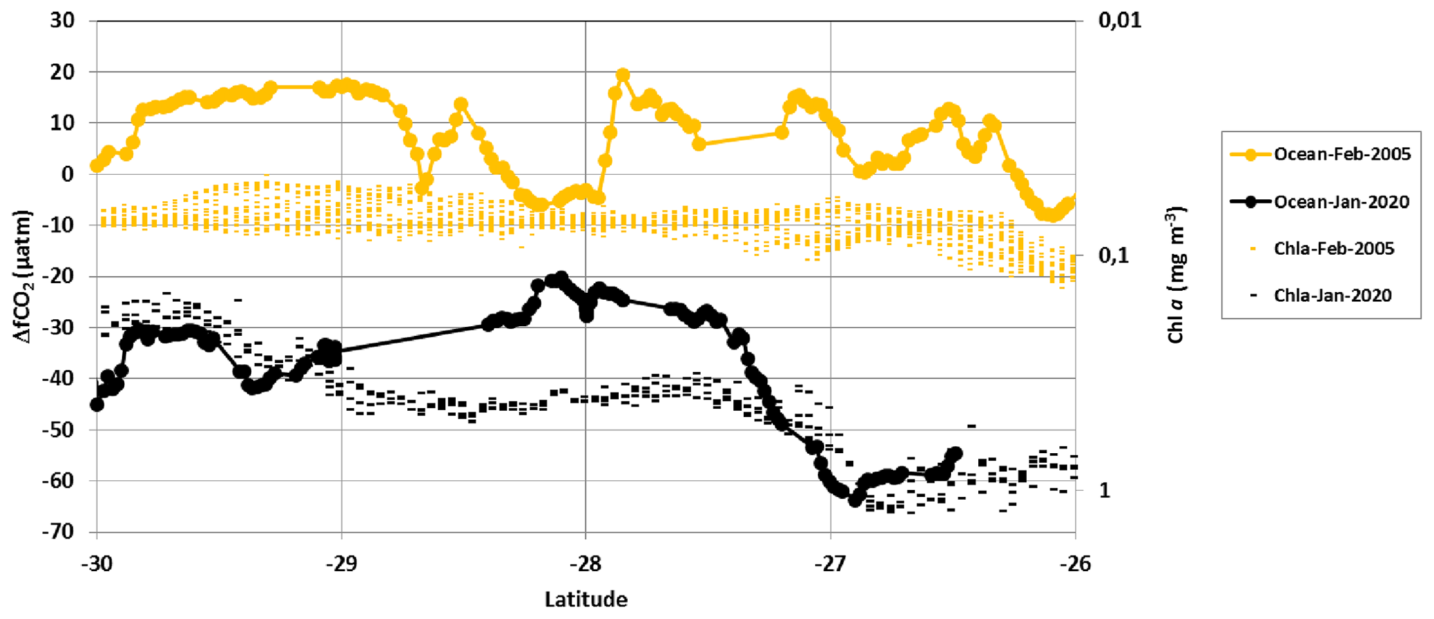
Figure 4 ΔfCO₂ (µatm) ($\mathrm{\Delta }f{\mathrm{CO}}_{\mathrm{2}}=f{\mathrm{CO}}_{\mathrm{2}}^{\mathrm{oce}}-f{\mathrm{CO}}_{\mathrm{2}}^{\mathrm{atm}}$) and sea surface Chl a (mg m⁻³) distribution in January 2020 (black) and February 2005 (orange) along the same track around 54^∘ E in the south-western Indian Ocean. Here Chl a is in log₁₀ scale and inverted. In 2020 when the SEMB was particularly strong, ΔfCO₂ was negative (ocean CO₂ sink), whereas in 2005 when the bloom was small, ΔfCO₂ was close to 0 or positive (ocean CO₂ source).

Table 2 Mean sea surface properties observed along the same track in January 2020 and February 2005 in the region 30–26^∘ S, 54^∘ E. Also indicated are the mean values in the same region and season from the climatology of Takahashi et al. (2014) and the Chl a climatology evaluated for January–February 1998–2019. The number of observations for SST, SSS and fCO₂ is indicated. Standard deviations are indicated in brackets.

The average monthly wind speed was also about the same in 2020 (7.9 m s⁻¹) and 2005 (8.5 m s⁻¹) (Fig. S5b). Consequently the difference in the air–sea CO₂ flux between the two periods was controlled by ΔfCO₂. In the region 26–30^∘ S, 55^∘ E, the mean CO₂ flux in 2005 was estimated at +1.2 mmol m⁻² d⁻¹ (a source) compared to −4.3 mmol m⁻² d⁻¹ (a sink) in 2020.

5 Discussion

5.1 A large biologically driven fCO₂ negative anomaly in 2020 relative to the anthropogenic uptake of CO₂

Like for fCO₂, the N-C_T concentrations observed in the SEMB in January 2020 (1950 µmol kg⁻¹, Fig. 3b, Table 1) were low compared to the climatology (Takahashi et al., 2014). At 24–28^∘ S, 54^∘ E, the N-C_T climatological value in January ranged between 1970 and 1980 µmol kg⁻¹. As the climatology produced by Takahashi et al. (2014) was referred to the nominal year of 2005, one would expect to observe higher N-C_T concentrations in 2020 due to anthropogenic CO₂ uptake.

In the Indian Ocean the decadal change of anthropogenic CO₂ (C_ant) was first evaluated by Peng et al. (1998) comparing data obtained in 1978 and 1995 north of 20^∘ S. For the upper layer in the tropics (20–10^∘ S), Peng et al. (1998) estimated an increasing rate of C_ant of around 1.1 µmol kg⁻¹ yr⁻¹. More recently, Murata et al. (2010) evaluated the changes of C_ant concentrations between 1995 and 2003 in the subtropics of the southern Indian Ocean. They estimated a mean increase of C_ant of +7.9 (±1.1) µmol kg⁻¹ over 8.5 years in the upper layers, corresponding to a trend of +0.93 (±0.13) µmol kg⁻¹ yr⁻¹. In a global context, Gruber et al. (2019a, b) estimated an accumulation of anthropogenic CO₂ (C_ant) of +14.3 (±0.3) µmol kg⁻¹ in surface waters of the south-western Indian Ocean over 1994–2007, corresponding to an increasing rate in C_ant of +1.10 (±0.02) µmol kg⁻¹ yr⁻¹. To confirm these C_ant trends that were based on the C_ant differences between two periods (1995–1978, 2003–1995 or 2007–1994), we calculated the C_ant concentrations and long-term trend using water column data available in 1978–2020 in the region 30–26^∘ S, 55^∘ E. We extracted the data from the most recent GLODAP (Global Ocean Data Analysis Project) quality-controlled data product (GLODAPv2.2021, Lauvset et al., 2021a, b), completed with data from OISO cruises in 2012–2018. To calculate C_ant we used the TrOCA (Tracer combining Oxygen, inorganic Carbon, and total Alkalinity) method developed by Touratier et al. (2007). Because indirect methods are not suitable for evaluating C_ant concentrations in surface waters due to gas exchange and biological activity, we selected the data in the layer 100–250 m below the DCM. C_ant concentrations were calculated for each sample in that layer and then averaged for each period to estimate the trend (Fig. 5). As expected the C_ant concentrations in the subsurface increased significantly from 1978 to 2020, and the long-term trend of +1.05 (±0.08) µmol kg⁻¹ yr⁻¹ over this period is close to previous estimates based on different periods and approaches (Peng et al., 1998; Murata et al., 2010; Gruber et al., 2019a).

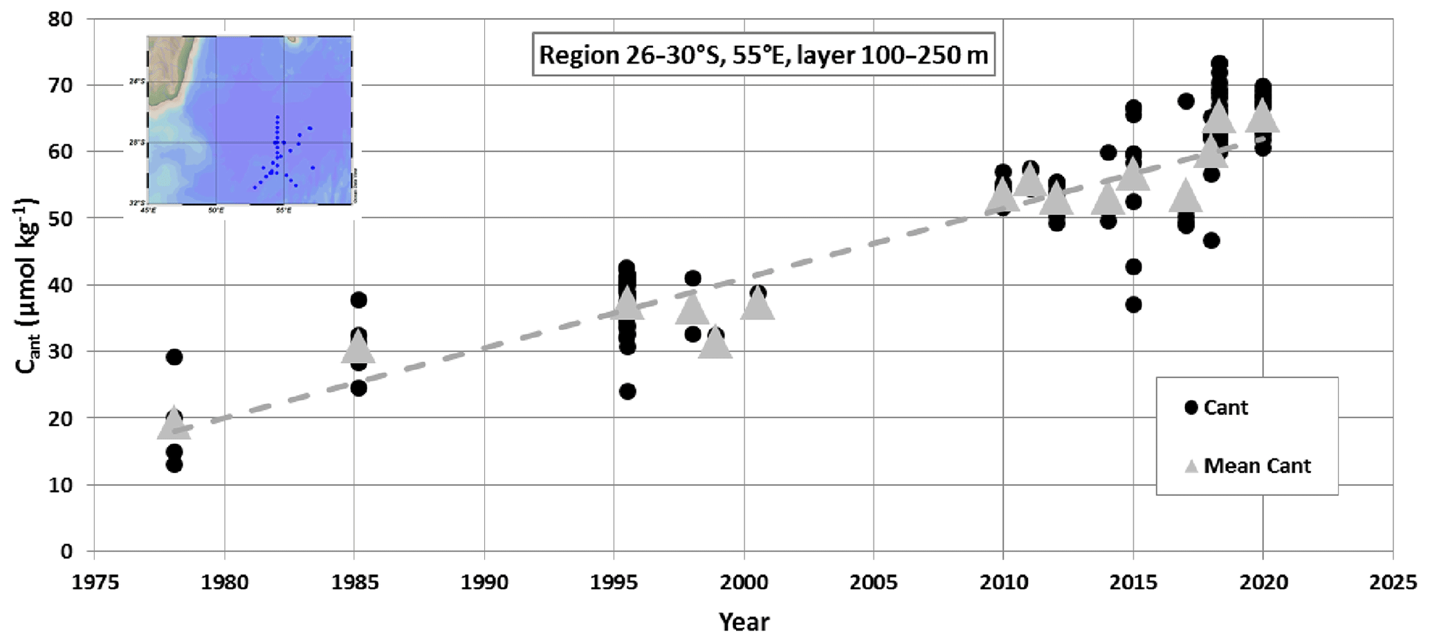
Figure 5 Time series of anthropogenic CO₂ concentrations (C_ant) estimated in the subsurface (layer at 100–250 m) in the region 26–30^∘ S, 55^∘ E from the GLODAPv2.2021 data product (Lauvset et al., 2021a, b) completed with OISO cruises in 2012–2018 (location of selected stations in the insert map). The figure shows the C_ant concentrations calculated for each sample (black dots) and the C_ant averaged in the layer at 100–250 m for each period (grey triangles). Over the period 1978–2020, the C_ant long-term trend is +1.05 (±0.08) µmol kg⁻¹ yr⁻¹ (dashed grey line).

Furthermore the C_ant trend of around +1 µmol kg⁻¹ yr⁻¹ is coherent with an increase in C_T of between +0.93 and +1.17 µmol kg⁻¹ yr⁻¹ derived from the oceanic fCO₂ increase over the period 1991–2007 estimated from winter and summer fCO₂ data (+1.75 and +2.2 µatm yr⁻¹ respectively, Metzl, 2009) assuming constant alkalinity and temperature. With the new data available after 2007, we have revisited the fCO₂ long-term trend by selecting only the austral summer data in the region around 27^∘ S, 55^∘ E (Fig. 2). For the period 1991–2019 we estimated an fCO₂ trend of +1.55 (±0.40) µatm yr⁻¹. This is less than the atmospheric fCO₂ increase of +1.89 (±0.03) µatm yr⁻¹ over the same period, suggesting that the CO₂ sink increased at this location. In a broader context, Landschützer et al. (2016) suggested that the carbon uptake tended to increase slightly in 1998–2011 in the subtropical Indian Ocean (their Fig. 3). We will see that such a change in the CO₂ fluxes in this region is also revealed in the CMEMS-LSCE-FFNN model (Chau et al., 2022). Note that if at 27^∘ S, 55^∘ E (Fig. 2) the ocean fCO₂ data in 2020 were also used to estimate the trend (1991–2020), the rate of fCO₂ would be only +1.09 (±0.48) µatm yr⁻¹, i.e. about half the atmospheric fCO₂ trend. The fCO₂ observations in 2020 represent a large negative anomaly at the local scale, and thus caution is needed when incorporating such an anomaly to detect and interpret long-term change in the CO₂ sink, at least in the south-western subtropical Indian Ocean.

To compare the fCO₂ trends listed above with the anthropogenic rate of around +1.0 µmol kg⁻¹ yr⁻¹ (Fig. 5), we have calculated C_T from the fCO₂ data and A_T derived from salinity (described below). For this calculation we used the CO2SYS programme (CO2SYS_v2.5, Orr et al., 2018) developed by Lewis and Wallace (1998) and adapted by Pierrot et al. (2006) with K₁ and K₂ dissociation constants from Lueker et al. (2000) and the KSO₄ constant from Dickson (1990). The total boron concentration is calculated according to Uppström (1974). For nutrients we fixed phosphate concentrations at 0 and silicate at 2.0 (±0.6) µmol kg⁻¹ (the mean of 79 surface observations measured during previous OISO cruises in the region 22–30^∘ S). To derive A_T from salinity we used the surface A_T observations obtained since 1998 in the subtropical south-western Indian Ocean (OISO cruises). From these data we estimated a robust relationship (Fig. 6):

$$\begin{array}{}\text{(3)}& \begin{array}{rl}{A}_T& \left(\mathrm{\mu }\mathrm{mol}{\mathrm{kg}}^{-\mathrm{1}}\right)=\mathrm{62.1601}\cdot \mathrm{SSS}+\mathrm{123.1}\\ & \left(\mathrm{rms}=\mathrm{7.0}\mathrm{\mu }\mathrm{mol}{\mathrm{kg}}^{-\mathrm{1}},r=\mathrm{0.89},n=\mathrm{3400}\right).\end{array}\end{array}$$

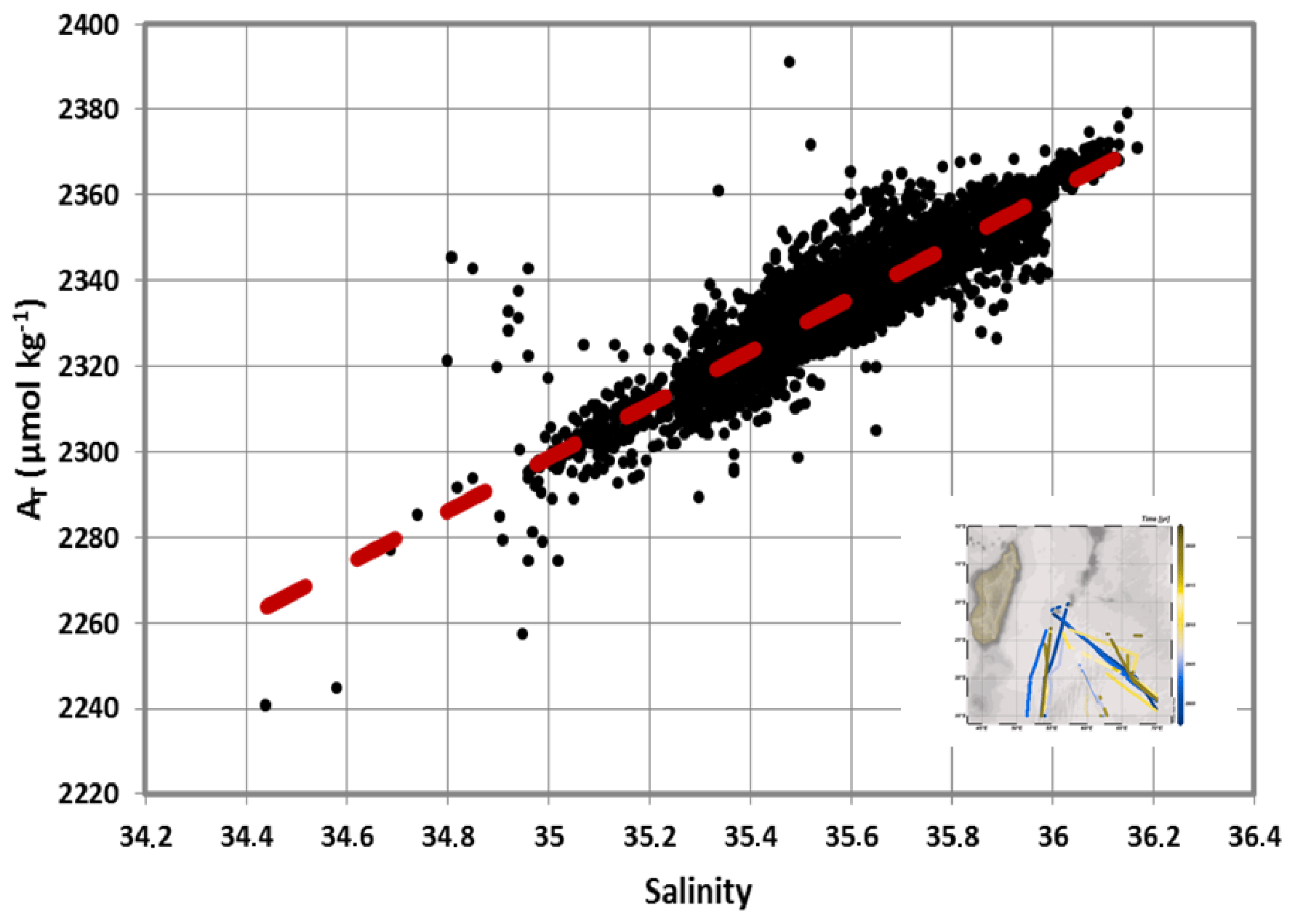
Figure 6 Relationship of A_T (µmol kg⁻¹) versus salinity deduced from surface A_T data (n=3400) obtained during OISO cruises in 1998–2020 in the south-western Indian Ocean. For the subtropics we have selected the data in the region 35–20^∘ S, 50–70^∘ E (track of cruises shown in the insert map). The relationship (red dashed) is $A_{\mathrm{T}}=\mathrm{62.1601}\cdot$ SSS + 123.1 and is used to calculate C_T concentrations in this region (Fig. 7). A_T data are available at NCEI OCADS (https://www.ncei.noaa.gov/access/ocean-carbon-data-system/oceans/VOS_Program/OISO.html, last access: 3 March 2022).

The use of other relationships (e.g. Millero et al., 1998; Lee et al., 2006) would slightly change the A_T concentrations but not the interpretation on the C_T trend in this region. The time series of salinity-normalized C_T (N-C_T= $C_{\mathrm{T}}\times \mathrm{35}/\mathrm{SSS}$) at 27–28^∘ S, 55^∘ E shows that N-C_T increased over the period 1991–2019 at a rate of +0.70 (±0.24) µmol kg⁻¹ yr⁻¹ (Fig. 7). This is somehow lower than the anthropogenic trend of +1 µmol kg⁻¹ yr⁻¹, suggesting that in addition to the anthropogenic CO₂ uptake, natural processes could also have a small impact on the C_T and fCO₂ trends in surface waters over almost 30 years.

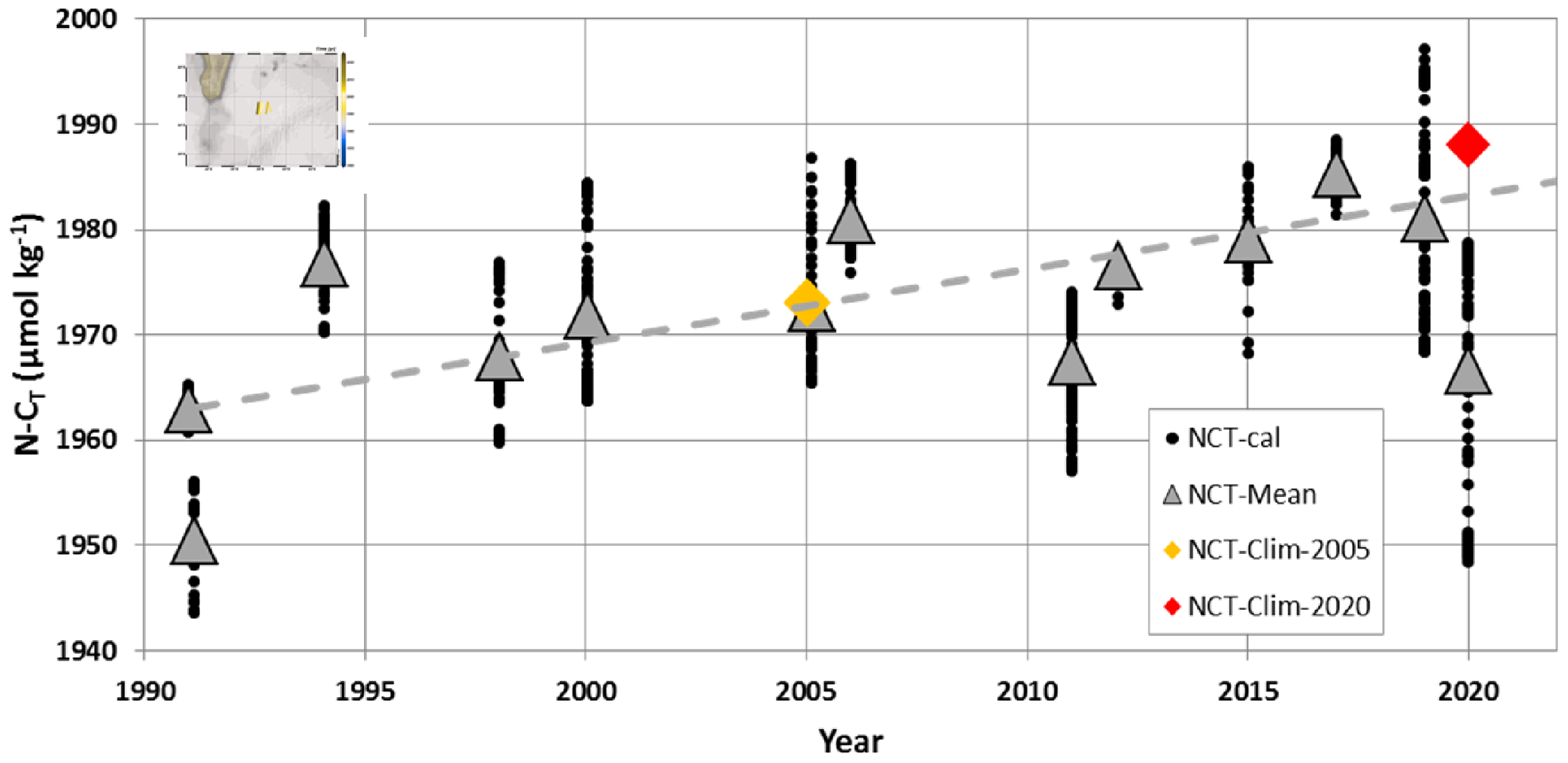
Figure 7 Time series of salinity-normalized C_T (N-C_T, black dots) and their monthly mean (grey triangles) at 27–28^∘ S, 55^∘ E (insert map) calculated with fCO₂ observations (see Fig. 2) and reconstructed A_T from salinity (Fig. 6). The figure shows data for the months of January and February (data available from 1991 to 2020 for austral summer). Over the period 1991–2019, the N-C_T trend is +0.70 (±0.24) µmol kg⁻¹ yr⁻¹ (dashed grey line), reflecting in part the anthropogenic CO₂ uptake. Note the low N-C_T in January 2020 in the SEMB compared to previous years with some values around 1950 µmol kg⁻¹ in 2020 as low as N-C_T calculated in 1991. The N-C_T concentration in the same region derived from the climatology of Takahashi et al. (2014) is also plotted (orange diamond for the reference year of 2005) as well as the climatological value for the year 2020 after correcting for anthropogenic CO₂ (red diamond).

Having an estimate of the C_T change due to anthropogenic CO₂ (around +1 µmol kg⁻¹ yr⁻¹) and taking into account this effect, the climatological N-C_T concentration of 1973 µmol kg⁻¹ for 2005 (Takahashi et al., 2014) corrected for the year 2020 would be 1988 µmol kg⁻¹ in the region of interest. This is higher by up to +36 µmol kg⁻¹ than the observed N-C_T in January 2020 in the SEMB (Table 1, Fig. 7). When correcting the climatological value to the observed C_T trend of +0.7 µmol kg⁻¹ yr⁻¹, the N-C_T in 2020 would be 1983.5 µmol kg⁻¹, i.e. +32.5 µmol kg⁻¹ higher than the observed value in January 2020. The N-C_T anomaly in January 2020 is also large compared to the mean N-C_T seasonal amplitude of 20 µmol kg⁻¹ generally observed in the subtropics of the southern Indian Ocean (Metzl et al., 1998; Takahashi et al., 2014). We also note that climatological N-A_T concentrations of 2295 µmol kg⁻¹ for January (Takahashi et al., 2014) are very close to those we observed in January 2020 (Table 1, Fig. 3b). Therefore the low fCO₂ and strong CO₂ sink in 2020 in the SEMB is due to a large drawdown of C_T, i.e. not driven by temperature changes or alkalinity.

5.2 Specificities of the SEMB in 2020

Based on previous studies it is likely that the biologically driven reduction of C_T in the SEMB under depleted sea surface nitrate concentrations was associated with the process of N₂ fixation (Uz, 2007). The hypothesis that diazotrophy would play a role in the temporal C_T (and thus fCO₂) variability is supported by the observation of large N₂-fixing phytoplankton in the SEMB region in 2005 during the MadEx cruise (Poulton et al., 2009). These authors found that the filamentous cyanobacteria Trichodesmium was most abundant south of Madagascar (over the Madagascar Ridge), whereas diatom–diazotroph associations (such as Rhizosolenia–Richelia) were mainly observed east of Madagascar (in the Madagascar Basin).

Our measurements in January 2020 showed high spatial variability of the N₂ fixation rate (range from 0.8 to 18.3 nmol N L⁻¹ d⁻¹, Fig. 8). Such variability in the subtropical Indian Ocean was also recently reported by Hörstmann et al. (2021), who measured N₂ fixation rates between 0.7 and 7.9 nmol N L⁻¹ d⁻¹ in January–February 2017 in the same region (OISO-27 cruise) but when the SEMB was not pronounced (Fig. 1b, c) and when fCO₂ was high and above equilibrium (Fig. 2). Our results for silicate (Si) and N₂ fixation observations are difficult to interpret because few samples were collected along the track (Fig. 8). A maximum of the N₂ fixation rate was observed at 30^∘ S that was not linked to changes in other properties. This local high N₂ fixation rate could be related to Trichodesmium species, but it was not sampled in January 2020. We also noted low Si concentrations at 27^∘ S (0.6 µmol kg⁻¹) associated with higher Chl a and lower fCO₂ and C_T (Fig. 3). The low silicate might be associated with the presence of diatom–diazotroph associations (DDAs) as observed during the MadEx cruise (Poulton et al., 2009). In the bloom, N₂ fixation increased northward from 28^∘ S (factor of ∼5). Based on measurements for different size fractions we observed that the N₂ fixation is mainly related to the fraction >20 µm (i.e. Trichodesmium and DDA) representing 88 % (±9 %) of the N₂ fixation. “Hotspots” of large diazotrophs (20–180 and 180–2000 µm) were also detected in other regions of the south-western Indian Ocean in May 2010 during the Tara expedition (Pierella Karlusich et al., 2021).

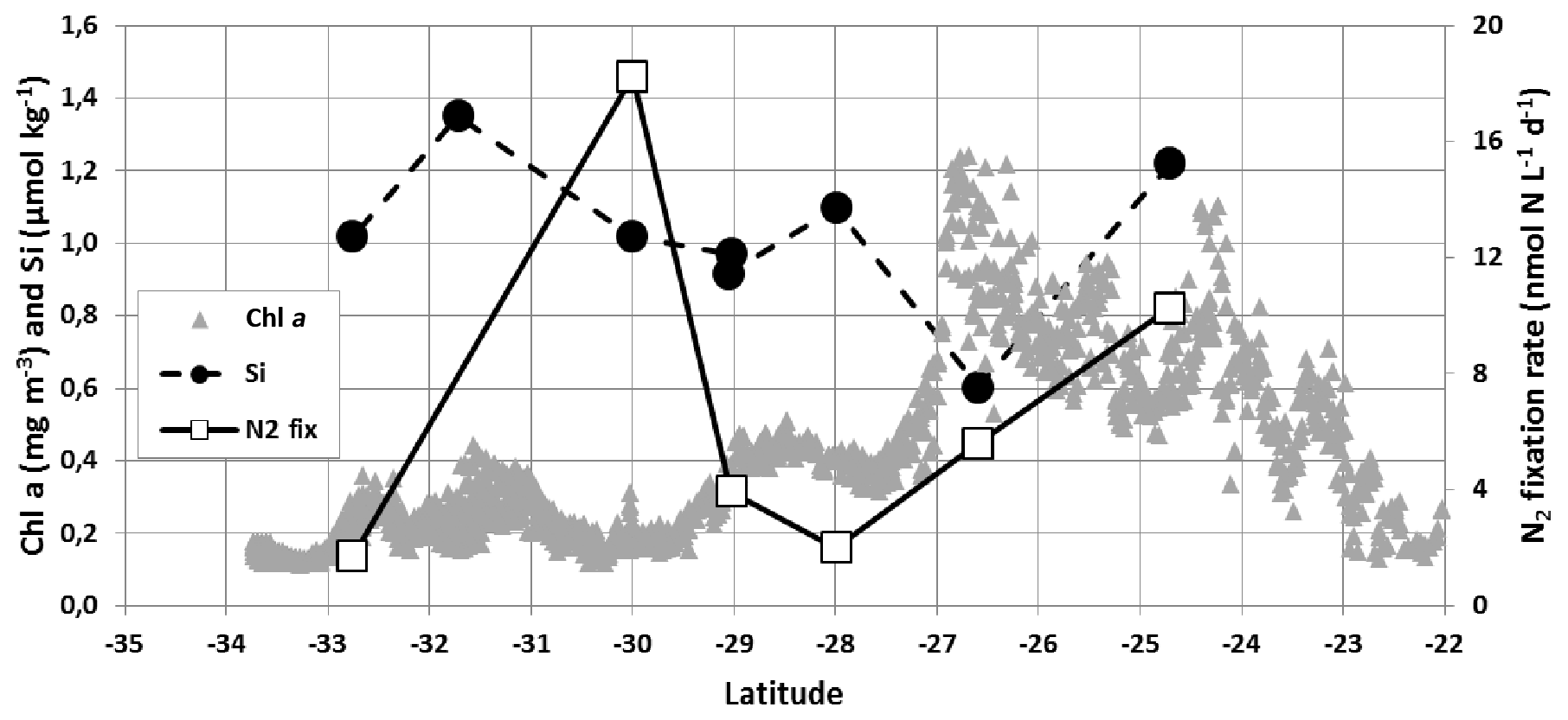
Figure 8 Sea surface silicate concentration (Si, µmol kg⁻¹, black circles, scale on the left), N₂ fixation rate (N₂ fix, nmol N L⁻¹ d⁻¹, open squares, scale on the right) measured in January 2020 (OISO-30 cruise) and Chl a (mg m⁻³, grey triangles, scale on the left) from MODIS (4 km × 4 km) along the cruise track. The low Si concentration (0.6 µmol kg⁻¹) recorded around 27^∘ S was linked to higher Chl a (up to 1.2 mg m⁻³) in the SEMB.

At a global scale, the presence of N₂ fixers in the south-western Indian Ocean has been detected from satellite data (Westberry and Siegel, 2006; Qi et al., 2020), and relatively high N₂ fixation rates in austral summer in this region were also derived from N₂ fixation data using a machine learning approach (Tang and Cassar, 2019; Tang et al., 2019). A large-scale distribution of diazotrophy was further estimated from surface C_T observations, suggesting the presence of N₂ fixers in the Mozambique Channel and the south-western Indian Ocean (Lee et al., 2002; Ko et al., 2018). These authors used regional relationships of N-C_T versus SST to reconstruct the N-C_T field from which they estimated the net carbon production (NCP) in nitrate depleted waters, a proxy for carbon production by N₂-fixing microorganisms. The N-C_T–SST relationship observed from in situ data in January 2020 somehow mimics this process (Fig. 9); i.e. the inter-annual variability of the N-C_T–SST relationship would also inform the NCP by N₂ fixers.

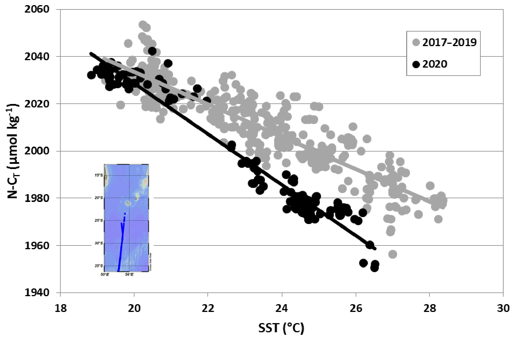
Figure 9 The relationship between N-C_T (µmol kg⁻¹) and SST in surface waters based on OISO cruises observations in the south-western Indian Ocean in austral summer 2017, 2018, 2019 and 2020 along the same repeated track (insert map). In January 2020 during the strong SEMB, the N-C_T–SST relationship (black dots and black line) was much sharper than in 2017–2019 (grey dots and grey line), indicative of N₂ fixation production in nitrate depleted waters (e.g. Ko et al., 2018).

Sea surface warming and shallow mixed-layer depth (MLD) are proposed to lead to optimal conditions for the growth of the N₂ fixers and generate the SEMB (e.g. Longhurst, 2001; Srokosz et al., 2015). In austral summer 2020, the ocean was not much warmer than previous years, suggesting that temperature was not a specific driver of the SEMB that year. To the contrary, in January 2020 the region experienced a particularly shallow MLD which might have favoured the bloom (observed MLD around 20 m at 27–28^∘ S, Figs. S8 and S9 in the Supplement).

As noted above, the strong bloom started in November 2019 and could be well identified in two large rings (Fig. S1). In the northern ring at 25^∘ S, 52^∘ E, the MLD was deep (>80 m) during 3 consecutive months in July–September 2019 and deeper compared to previous years (Fig. S10 in the Supplement). This would have injected nutrients (and maybe iron) in surface layers, and when the MLD was shallow at that location (<20 m) the bloom developed in November 2019 and reached high Chl a values in December 2019 (up to 1.8 mg m⁻³). As the bloom covered a large region in December 2019 and January 2020, other specific processes like iron supply (from dust, coastal zone, rivers or sediments) still need to be identified to fully explain 2020 SEMB dynamics. The 2020 bloom was clearly recognized in Chl a, fCO₂ and C_T observations, but at that stage we have no clear explanation on the process (or multiple drivers) that generated its extent and intensity.

5.3 The changing ocean CO₂ uptake in the SEMB based on reconstructed pCO₂

The results presented above were based on local underway fCO₂ observations, and the integrated air–sea CO₂ fluxes were thus extrapolated from local data on a surface representing the area covered by the bloom leading to a carbon uptake of between −1.7 and −2.7 TgC per month in January 2020. In the domain 25–30^∘ S, 50–60^∘ E we estimated a CO₂ sink in January 2020 close to −1 TgC per month.

Figure 10 Maps of Chl a (mg m⁻³), pCO₂ (µatm) and the air–sea CO₂ fluxes (mmol m⁻² d⁻¹) in the south-western Indian Ocean in December 2018 (left) and December 2019 (right). In December 2019 when the SEMB was particularly strong, the pCO₂ was lower, and air–sea CO₂ fluxes were negative (ocean sink, in blue), whereas in December 2018 when the bloom was small, the fluxes were near equilibrium or positive in this region (ocean source, yellow-brown). Chl a data downloaded from https://resources.marine.copernicus.eu/ (OCEANCOLOUR_GLO_CHL_L4_REP_OBSERVATIONS_009_093, last access: 10 April 2021). Figures produced with ODV (Schlitzer, 2013).

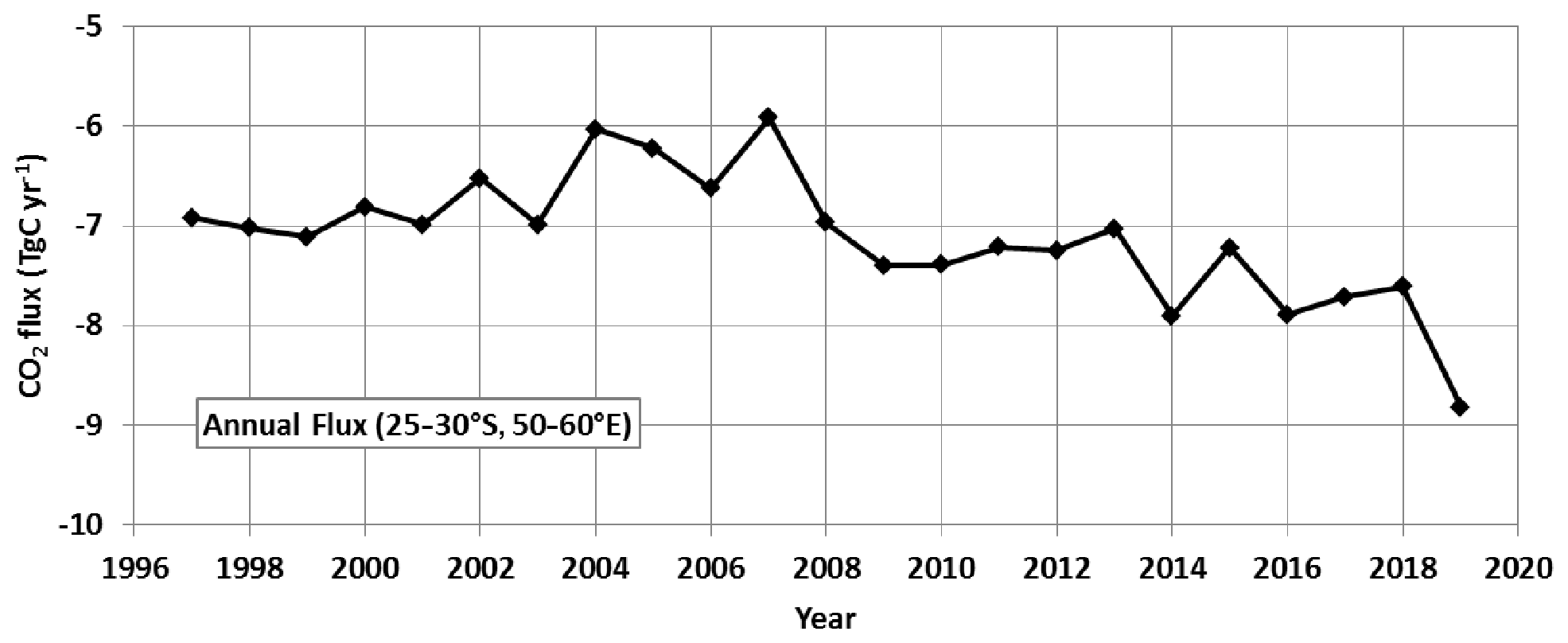
Figure 11 Annual air–sea CO₂ flux (TgC yr⁻¹) in the south-western Indian Ocean (region of 25–30^∘ S, 50–60^∘ E) for the period 1996–2019 from the CMEMS-LSCE-FFNN model. The carbon uptake progressively increased after 2007 with a maximum CO₂ sink estimated in 2019 when the SEMB was particularly strong.

To evaluate the impact of the bloom at the regional scale, we used monthly surface ocean pCO₂ and air–sea CO₂ flux fields reconstructed by a neural network method as described in Sect. 3 (CMEMS-LSCE-FFNN, Chau et al., 2022). The SEMB was well developed in December 2019, and we can evaluate its impact on the air–sea CO₂ fluxes by comparing December 2018 (low bloom) and December 2019 (strong bloom, Fig. 10). In the region 25–30^∘ S, 50–60^∘ E, the average pCO₂ in December 2019 (375.9±6.3 µatm) was much lower than in December 2018 (396.6±6.0 µatm) and thus opposite of the expected pCO₂ increase due to anthropogenic CO₂ uptake. At the local scale, within the bloom at 27^∘ S, 54^∘ E or at 29^∘ S, 50^∘ E, the CMEMS-LSCE-FFNN model estimated low pCO₂ clearly linked to higher Chl a in December 2019 (Figs. S11 and S12 in the Supplement). Consequently the region was a small CO₂ source of +0.07 (±0.53) mmol m⁻² d⁻¹ in December 2018 but a CO₂ sink in December 2019 of −3.1 (±1.0) mmol m⁻² d⁻¹. Integrated over the region 25–30^∘ S, 50–60^∘ E the carbon uptake changed from a small CO₂ source in December 2018 of +0.019 TgC per month to a CO₂ sink in December 2019 of −0.8 TgC per month (Fig. S13 in the Supplement), close to the estimate derived from observations in January 2020 (−1.0 TgC per month). Over the period 1996–2018, each year the model evaluates a CO₂ source in December averaging +0.12 (±0.10) TgC per month. This suggests that in late 2019 the CMEMS-LSCE-FFNN model did capture the effect of the SEMB on pCO₂ and CO₂ fluxes, leading to a stronger regional CO₂ annual sink in 2019 (−8.8 TgC yr⁻¹) compared to previous years (Fig. 11). A major SEMB was previously recognized in 1999, 2006 and 2008 (Dilmahamod et al., 2019; see also Fig. 1). The model overestimates the CO₂ sink in 2006 and 2008 but surprisingly not in 1999 (Fig. 11). This is probably because the ocean was warmer from December 1998 to March 1999, inducing a positive anomaly of fCO₂ that would balance the decrease of fCO₂ due to the biological activity in summer 1999. With the exception of 2008 when the SEMB was also strong (Fig. 1), the CO₂ sink anomalies in 1998–2018 appeared relatively modest compared to that observed in 2019 (Fig. 11).

6 Conclusions

The new observations in the south-western Indian Ocean presented here showed that the fCO₂ and C_T concentrations in January 2020 have been very low and far from normal conditions since 1991. This is explained by the strong SEMB event that started in November 2019 in this region and was well developed in December 2019 and January 2020. Thanks to the continuous ocean colour satellite data since 1997, the time series of Chl a in this region showed that the bloom was particularly strong in austral summer 2019/20. We suspect that prior to 1997, the SEMB had been less intense as suggested by in situ fCO₂ data in 1991–1994 (Fig. 2). We estimated that the SEMB led to a regional carbon uptake of between −1.7 and −2.7 TgC per month in January 2020. The variation of the regional ocean CO₂ sink due to the SEMB developed in late 2019 was also quantified with the CMEMS-LSCE-FFNN model. Model results indicate a large anomaly in December 2019 that led to an annual sink of −8.8 TgC yr⁻¹, i.e. about 1 TgC yr⁻¹ larger than previous years. The strong bloom in austral summer 2020 represents an interesting benchmark case to test models for a better understanding of the origin of the SEMB and its impact on the regional ocean CO₂ sink. Future studies should target sensitivity analysis with complex biogeochemical models including the CO₂ system, at different spatial resolution for the dynamics and with (or without) N₂ fixers (e.g. Monteiro et al., 2010; Landolfi et al., 2015; Paulsen et al., 2017). This plankton functional type is not yet included in models dedicated to this region (Srokosz et al., 2015; Dilmahamod et al., 2020). The new fCO₂, C_T, A_T and N₂ fixation rate observations presented here along with historical data (e.g. SOCAT, Bakker et al., 2016, 2021; Fig. 2) could serve as a validation to compare periods with or without bloom. In the future, if the SEMB as observed in 2020 is more frequent or becomes a regular situation and if organic matter is exported below the surface mixed layer, this could represent a negative feedback to the ocean carbon cycle; i.e. the ocean sink would be enhanced. As already noted by several authors (e.g. Dilmahamod et al., 2019), dedicated studies in this region at the scale of eddies coupling dynamical and biological processes, including not only the sampling of plankton and nutrients (e.g. iron) but also the determination of rates (e.g. N₂ fixation), would be relevant to understanding the processes controlling the SEMB and to evaluating its impact on the biological carbon pump.