Species richness and functional attributes of fish assemblages across a large-scale salinity gradient in shallow coastal areas

Coastal ecosystems are biologically productive, and their diversity underlies various ecosystem services to humans. However, large-scale species richness (SR) and its regulating factors remain uncertain for many organism groups, owing not least to the fact that observed SR (SR_obs) depends on sample size and inventory completeness (IC). We estimated changes in SR across a natural geographical gradient using statistical rarefaction and extrapolation methods, based on a large fish species incidence dataset compiled for shallow coastal areas (<30 m depth) from Swedish fish survey databases. The data covered a ca. 1300 km north–south distance and a 12-fold salinity gradient along sub-basins of the Baltic Sea plus the Skagerrak and, depending on the sub-basin, 4 to 47 years of samplings during 1975–2021. Total fish SR_obs was 144, and the observed fish species were of 74 % marine and 26 % freshwater origin. In the 10 sub-basins with sufficient data for further analysis, IC ranged from 77 % to 98 %, implying that ca. 2 %–23 % of likely existing fish species had remained undetected. Sample coverage exceeded 98.5 %, suggesting that undetected species represented <1.5 % of incidences across the sub-basins, i.e. highly rare species. To compare sub-basins, we calculated standardized SR (SR_std) and estimated SR (SR_est). Sub-basin-specific SR_est varied between 35 ± 7 (SE) and 109 ± 6 fish species, being ca. 3 times higher in the most saline (salinity 29–32) compared to the least saline sub-basins (salinity < 3). Analysis of functional attributes showed that differences with decreasing salinity particularly reflected a decreasing SR of benthic and demersal fish, of piscivores and invertivores, and of marine migratory species. We conclude that, if climate change continues causing an upper-layer freshening of the Baltic Sea, this may influence the SR, community composition and functional characteristics of fish, which in turn may affect ecosystem processes such as benthic–pelagic coupling and connectivity between coastal and open-sea areas.

1 Introduction

Biodiversity is essential for ecosystem processes and ultimately for the humans depending on these (IPBES, 2019). Coastal ecosystems are often biologically diverse and highly productive, providing valuable ecosystem services to humans, such as food, water purification and protection against floods (Griffiths et al., 2017; Kraufvelin et al., 2018; Pan et al., 2013). However, threats to coastal biodiversity from, for example, overfishing, habitat loss, pollution, eutrophication and climate change are many and profound (Duncan et al., 2015; Griffiths et al., 2017; Pan et al., 2013). At the same time, the number of species occurring in coastal habitats often remains uncertain (Appeltans et al., 2012), making improved understanding of coastal biodiversity especially important to support conservation and management measures (Pan et al., 2013; Rooney and McCann, 2012).

Taxonomic inventories, or species censuses, are required, for example, for the analysis of biodiversity patterns, delineation of species ranges and prioritization of conservation efforts (Mora et al., 2008). Species richness (SR), i.e. the number of species in an ecosystem, is a classical indicator of biodiversity, also referred to as “alpha diversity” (Gotelli and Colwell, 2001; Hill, 1973). However, since achieving complete species inventories is often impracticable with realistic sample efforts, most censuses remain incomplete, and many rare species remain unknown. Consequently, it is important to consider the effect of sample size and inventory completeness (IC) on observed SR (SR_obs) to avoid biased or misleading comparisons or interpretations (Chao and Chiu, 2016; Chao et al., 2020; Colwell and Coddington, 1994; Mora et al., 2008).

SR is connected to several ecosystem processes, such as productivity (Duffy et al., 2017), and the efficiency of resource use and nutrient cycling. SR may also facilitate the simultaneous provision of several ecosystem processes, i.e. an ecosystem's multifunctionality (Byrnes et al., 2014). However, since species do not contribute equally to ecosystem functioning, the diversity of species functional attributes adds another important dimension to ecosystem understanding (Duncan et al., 2015; Reiss et al., 2009). Functional diversity can enhance long-term stability through functional redundancy and complementarity and can help to buffer ecosystems against disturbances (O'Gorman et al., 2011).

Salinity is a key variable influencing SR in coastal areas as natural differences in salinity among locations function as a threshold or “ecological barrier” for the distribution of freshwater and marine species, for example, in the Baltic Sea (Olenin and Leppäkoski, 1999; Vuorinen et al., 2015). At the same time, an on average intensified water cycle caused by global warming is changing the salinity regimes of marine and coastal ecosystems (Durack et al., 2012; Liblik and Lips, 2019; Meier et al., 2022). It is important to understand how salinity influences species distributions in aquatic ecosystems to be able to better predict how potential changes may affect ecosystem functioning.

The Baltic Sea, one of the world's largest brackish water bodies, exhibits a pronounced, geographically stable salinity gradient that is maintained by sporadic inflows of saline water from the North Sea through the Danish Straits and by freshwater input from large rivers, especially in the north. Hence, the Baltic Sea gradient can serve as a model on the influence of salinity on species distributions (Johannesson and Andre, 2006; Ojaveer et al., 2010). SR_obs is often higher at the more saline conditions, e.g. for macroalgae, benthic bacteria, and benthic meio- and macrofauna (Broman et al., 2019; Klier et al., 2018; Middelboe et al., 1997; Schubert et al., 2011). In other studies, SR_obs was highest at highest salinity, lowest at intermediate salinity and intermediate at lowest salinity, e.g. for phytoplankton and benthic macrofauna (Bonsdorff, 2006; Olli et al., 2019; Zettler et al., 2014), or there was no clear trend between SR_obs and salinity, e.g. for bacterio-, pico- and mesoplankton (Herlemann et al., 2016; Hu et al., 2016).

The species composition of fish in the Baltic Sea is regulated by salinity as well (Olsson et al., 2012; Pekcan-Hekim et al., 2016) even though other factors, such as temperature or habitat complexity, might also influence large-scale patterns of fish SR in estuaries (Vasconcelos et al., 2015; Schubert et al., 2011). In the Baltic Sea, fish SR_obs is generally higher in areas of higher compared to lower salinities (HELCOM, 2020; Hiddink and Coleby, 2012; Lappalainen et al., 2000; MacKenzie et al., 2007; Ojaveer et al., 2010; Pecuchet et al., 2016; Thorman, 1986). Various studies have also reported changes in fish SR_obs or species composition over time (e.g. Ammar et al., 2021; Törnroos et al., 2019). However, despite concerns that fish SR may decline in the future due to decreasing upper-layer salinity (e.g. MacKenzie et al., 2007; Pecuchet et al., 2016; Vuorinen et al., 2015), information on how the complete coastal fish assemblage varies spatially in relation to the Baltic Sea salinity gradient, including potential differences across functional groups, is lacking. Hence, there is a need to complement already existing information on the influence of salinity on various Baltic Sea organism groups with more complete information in relation to fish diversity, taxonomically and functionally. This kind of understanding for multiple trophic levels is needed to better understand and predict how changing salinity, in the Baltic Sea and in coastal areas in general (Durack et al., 2012; Liblik and Lips, 2019), may affect ecosystem structure and functioning (MacKenzie et al., 2007). For example, if different species groups are differently affected, this may also change biotic interactions such as benthic–pelagic coupling, with effects on exchanges of energy, mass or nutrients between benthic and pelagic habitats (Griffiths et al., 2017). Moreover, understanding SR at a broader, sub-regional scale is important to support analyses of potential SR and species compositions at more local scales within each sub-basin.

To this aim, we compiled a large dataset on fish species observations in shallow (<30 m depth) Swedish coastal areas, defined in alignment with the EU Marine Strategy Framework Directive as the area within 1 nmi, that is, 1852 m, beyond the national baseline (EC, 2017). The data compilation was based on multiple existing sources of Swedish mapping and monitoring combined over the years 1975–2021. The extensive dataset covered fish species incidence information from 1638 unique observations/fishing occasions, during which in total 21 670 species incidences were recorded. Geographically, the data covered 12 hydrographically distinct sub-basins and a ca. 12-fold salinity gradient from close to freshwater conditions in the inner Baltic Sea to close to fully marine conditions at the Swedish west coast. The annual mean water temperature varies ca. 2-fold across the same area. Since SR_obs is strongly dependent on sample size, which differed between sub-basins, we used statistical rarefaction and extrapolation methods to estimate IC and standardized SR per sub-basin. Further, we categorized each fish species according to origin (marine vs. freshwater), as well as three functional attributes based on coastal habitat preference, vertical preference and feeding habitat, and investigated the influence of salinity (and, for comparison, temperature) on fish SR in total and within the functional attributes. We discuss the results in the context of the regulating influence of salinity on fish SR and community composition in coastal ecosystems, as well as potential implications for conservation and ecosystem management.

2 Methods

2.1 Study system

The Baltic Sea, an enclosed, essentially non-tidal brackish marine region with maximum and mean depths of 460 and 54 m, respectively, and a water residence time of 25–40 years, is among the world's largest estuaries (area: 415 000 km²; HELCOM, 2018). Its current brackish conditions were formed by the gradual narrowing of its opening to the North Sea and have been in place for ca. 3000 years (Russell, 1985). Due to its geographically variable but locally relatively stable salinity conditions, the Baltic Sea has been called a “marine-brackish-limnic continuum” (Bonsdorff, 2006). Its surface salinity changes from <3 (psu) in the inner-most areas in the north and northeast to almost fully marine (ca. 29) in the Kattegat in the southwest (Table 1). Within this gradient, the Baltic Sea can be divided into hydrographically distinct sub-basins, mostly separated by shallow sounds or sills. To strengthen the database with respect to higher-salinity areas we additionally included a North Sea sub-basin adjacent to the Kattegat, i.e. the Skagerrak (salinity ca. 32; Table 1).

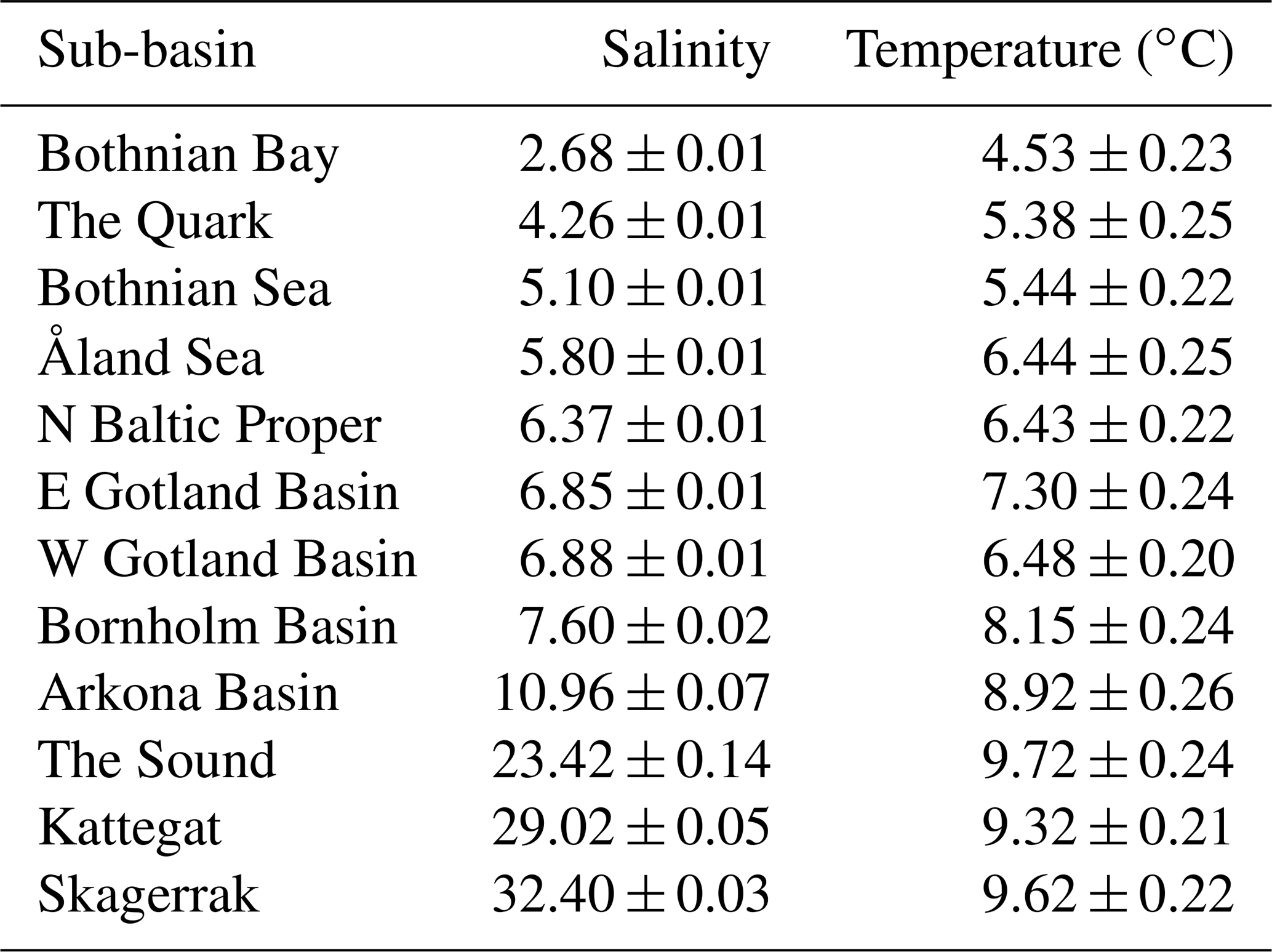
Table 1 Salinity and temperature in Swedish coastal areas, given as mean (± SE) annual values per sub-basin across the years 1993–2019. Values represent conditions near the bottom at 0–30 m depth based on data from the EU Copernicus Marine Service Information (CMEMS, 2021).

Reflecting its salinity conditions the Baltic Sea harbours a unique fish fauna with a mixture of freshwater species (e.g. northern pike (Esox lucius), perch (Perca fluviatilis), pikeperch (Sander lucioperca)) and marine species (e.g. cod (Gadus morhua), herring (Clupea harengus); Olsson et al., 2012). Further, many marine fish populations have adapted to the brackish conditions from their Atlantic counterparts (Laikre et al., 2005), for example, Baltic cod and herring populations, and one flounder species is endemic to the Baltic Sea (Momigliano et al., 2018). Hence, the Baltic Sea may also have a unique value as a refuge for evolutionary lineages and constitute an important genetic resource for management and conservation (Johannesson and Andre, 2006).

2.2 Species richness data

The primary source of fish species data was the Swedish National database of coastal fish (KUL; https://www.slu.se/kul, last access: 27 April 2021), which holds public, quality-assured data from surveys encompassing coastal fish monitoring, mapping projects and surveillance programmes over the entire salinity gradient of the Baltic Sea plus the Skagerrak. Coastal areas were delineated as the zone within one nautical mile beyond the national baseline (EC, 2017), as available from the Water Information System Sweden (“WISS”; https://viss.lansstyrelsen.se/Maps.aspx, last access: 10 November 2020, in Swedish), and KUL data records for 1975 to 2021 were extracted. Subsequently, data from shallow depths <30 m were selected, corresponding to the main represented sampling methods in the database (Table S1 in the Supplement) and approximately to the photic depth in the concerned coastal habitat types (Kaskela et al., 2012). This selection resulted in 154 172 data entries, i.e. individual fish that had been caught and identified to species by specialists, with the number of years with available data differing between sub-basins (Table S2). Further, quality-assured data were included from (1) a national coastal trawl survey (n=4420), (2) the ICES-coordinated International Bottom Trawl Survey (IBTS, n=1969) and (3) national projects using standardized methodology (n=893), all carried out in the Skagerrak, the Kattegat and the Sound, selecting only hauls from <30 m depth within the concerned geographical delineations (see above). Corresponding trawl data for the inner Baltic Sea area are not collected at depths <30 m in Swedish waters. Across databases, only sampling occasions with geographical coordinates and verified sampling references were included. Hence, data collected from multiple types of gear were combined, including gill nets, fyke nets, seines, trap nets, low-impact underwater detonations and trawls, in order to maximize the chance of including different species (Table S1). The ambition to collate information from all available fish surveys implied some differences in predominating data collection methods across the studied geographical range. The main data sources were trawls and trap net surveys in the most saline sub-basins, i.e. the Skagerrak, the Kattegat and the Sound, and gill net surveys in the remaining sub-basins (Table S1). While each gear has a specific selectivity and efficiency, a previous comparison of data from gill and fyke net samplings at the Swedish west coast did not reveal consistent differences in biodiversity metrics, and the statistical approaches were chosen to minimize a potential bias when comparing SR among sub-basins (Bergström et al., 2013; Chao et al., 2020; see also search of additional data sources below and Sects. 2.3 and 4).

Data on observed SR, SR_obs, were available for all 12 sub-basins (Table 2), representing between 4 and 47 years of data, depending on the sub-basin (Table S2). However, subsequent statistical analyses and comparisons were conducted only for the 10 sub-basins containing data from at least 30 sampling/fishing occasions, corresponding to several hundred fish incidences (i.e. Bothnian Bay, the Quark, Bothnian Sea, Åland Sea, northern Baltic Proper, western Gotland Basin, Bornholm Basin, the Sound, the Kattegat and the Skagerrak; see also Sect. 2.3). This dataset is hereafter referred to as “raw data”, and it contains in total 160 453 entries (i.e. fish individuals caught and determined to species) from 1638 sampling/fishing occasions at 4571 unique locations. Eastern Gotland Basin and Arkona Basin were not statistically analysed since we considered these sub-basins too under-sampled, with only 13 and 7 samplings, respectively, from 9 and 4 different years, and less than 100 species incidences in total (Tables 2, S2). Additionally, we searched for evidence of fish species that had remained undetected in the fish surveys (i.e. incidence database; see Sect. 2.3) by identifying fish species records from three additional sources using the same criteria for geographical and depth delineations of shallow coastal areas as above, i.e. (1) the national public database for citizens' reporting of species observations hosted by the Swedish University of Agricultural Sciences (SLU Swedish Species Information Centre, https://www.artportalen.se/ (last access: 27 April 2021); n=8926, unreasonable species observations deemed as falsely identified were discarded), (2) the national archive for oceanographic data hosted by the Swedish Meteorological and Hydrological Institute (SHARKweb, https://www.smhi.se/en/services/open-data/national-archive-for-oceanographic-data (last access: 27 April 2021); n=1259), and (3) published inventory data from the Skagerrak, the Kattegat and Bornholm Basin (Pihl and Wennhage, 2002; Pihl et al., 1994; Wikström A., 2009). These “additional data sources” were used as complementary information on SR_obs but could not be used in the statistical analysis since they did not have complete sampling and species incidence information. Further, our SR results were compared with the HELCOM (2020) checklist on macro-species containing information for all of the sub-basins and depths in the Baltic Sea region.

Table 2 Summary information for the fish incidence database and additional data sources, covering 12 sub-basins in Swedish shallow coastal areas (<30 m depth). Inventory completeness (IC), sample coverage (SC), standardized (SR_std) and estimated (SR_est) values were statistically estimated for sub-basins with a sample size of >30 fishing/sampling occasions. Of these, SR_std was calculated for a SC of 98.5 %, which was the lowest SC among sub-basins with sufficient data (i.e. Åland Sea). For comparison, the last two columns give SR_obs for Swedish shallow coastal areas when also including species records from additional data sources (not included in the statistical analyses; see Sect. 2.2) and for each Baltic Sea sub-basin according to HELCOM (2020), i.e. across depths and Baltic countries. NA: not applicable; n.d.: not determined.

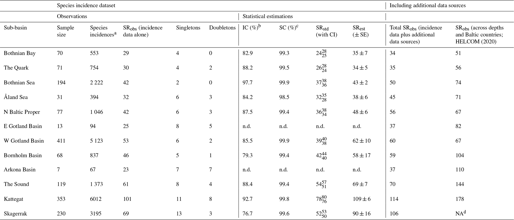
^a Sum of the number of unique species observed across all sampling occasions. Please note that this does not correspond to “entries” in Sect. 2.2, which is individual fish caught and determined to species.
^b Percentage of species detected from the estimated “true” (i.e. observed plus undetected) SR, i.e. 100⋅ SR${}_{\mathrm{obs}}/$ SR_est (Chao et al., 2020).
^c Percentage of incidences detected from the estimated “true” (i.e. observed plus undetected) incidences (Chao et al., 2020).
^d Not included in the Baltic Sea region.

2.3 Analysis of species richness data

The raw data were first summarized into a dataset of unique fish species caught in presence–absence format, per fishing/sampling occasion in each sub-basin, and then further aggregated to an incidence frequency format (Chao et al., 2014), in which incidence is occurrence/presence of a species. The resulting dataset gives the observed total incidence of each species over the number of fishing/sampling occasions per sub-basin and is referred to as “fish incidence database”. Each unique combination of a fishing/sampling location per date was defined as one sampling unit, and these were summed per sub-basin to obtain the sample sizes. Subsequently, incidence-based Hill diversity numbers of three “orders”, which differ in their propensity to include or exclude relatively rarer species (Hill, 1973), were calculated to quantify the species diversity of each assemblage, i.e. (1) species richness (SR), which counts all species equally irrespective their incidence frequency, (2) Shannon diversity (ShD), which considers the incidence frequency and can be interpreted as the effective number of frequent species, and (3) Simpson diversity (SiD), which can be interpreted as the effective number of highly frequent species (Chao et al., 2014, 2020). Calculations were performed using the R package iNEXT (Chao et al., 2020; Hsieh et al., 2016), and the values are hereafter referred to as observed SR, ShD and SiD, respectively. It should be noted that, using these methods, Shannon and Simpson diversities are expressed in terms of richness, i.e. number of species, which differs from other known formats. Specifically, ShD is the exponential of Shannon's entropy index, and SiD is the inverse of Simpson's concentration index (Chao et al., 2014).

SR_obs is highly dependent on “sample completeness” (Colwell and Coddington, 1994; Hill, 1973), and it typically underestimates the “true” SR due to undetected species, an aspect referred to as under-sampling, sampling bias or sampling problem (Chao et al., 2014; Chao and Jost, 2015; Menegotto and Rangel, 2018). Similar to Hill numbers, sample completeness can be calculated for different “orders” (Chao et al., 2020). The zero-order sample completeness is hereafter referred to as inventory completeness (IC). It is calculated as the ratio of SR_obs to the estimated “true” SR (i.e. observed plus undetected SR; see “estimated SR” below), hence giving the proportion of detected species without considering the species incidence frequencies. We calculated IC for the data merged over time and including resident as well as migrating and visiting fish species. The first-order sample completeness, hereafter referred to as “sample coverage” (SC), is a measure where species are weighted by their detection probabilities, giving the proportion of incidences detected from the estimated “true” incidences (Chao et al., 2020).

To correct for the effect of differing sample completeness on SR_obs and allow accurate, unbiased comparisons between sub-basins, we used a coverage-based rarefaction and extrapolation method implemented for incidence data in the R package iNEXT (Chao et al., 2014, 2020; Hsieh et al., 2016). A coverage-based method was chosen because more traditional sample-size-based corrections can introduce a systematic bias since the number of samples needed to fully characterize a community depends on its SR (Chao and Jost, 2012). For each sub-basin, we obtained (1) the rarefied SR, ShD and SiD, which were standardized to the minimum observed SC across all included sub-basins (hereafter referred to as standardized values, i.e. SR_std, ShD_std and SiD_std) and (2) the fish SR extrapolated to twice the actual sample size (hereafter referred to as estimated values, i.e. SR_est, ShD_est and SiD_est; Chao et al., 2014, 2020; Hsieh et al., 2016). Similar analyses were also conducted for SR of fish with different functional attributes (see Sect. 2.4). All calculations were conducted using R version 4.0.4 (R Core Team, 2021).

2.4 Fish functional attributes

All observed fish species were classified by origin (i.e., marine or freshwater) and assigned three functional attributes based on ecological and behavioural traits (Kullander, 2002). Specifically, the affinity of each species to different parts of the coastal habitat, or habitat preference, was assigned based on Elliott and Dewailly (1995) and Pihl and Wennhage (2002), however with certain adaptations to suit both marine and brackish conditions (Table S3–S4). Applied categories were as follows: catadromous or anadromous migrant (CA), using coastal habitats only when migrating between marine and freshwaters for spawning and feeding; marine juvenile migrant (MJ), using coastal habitats primarily as nursery or feeding grounds; marine visitor (MV), occurring irregularly in the coastal area, having their primary habitat in deeper waters; marine seasonal migrant (MS), making regular seasonal visits to coastal habitats, usually as adults; and coastal resident (CR), spending almost their complete life cycle in coastal habitats or the littoral coastal zone. The main vertical distribution of each species in the water column, considering the adult stage, was assigned based on Elliott and Dewailly (1995) and Koli (1990) as follows: pelagic (P), living mainly in the water column; demersal (D), mainly associated with the bottom substrate; demersal–pelagic (DP), alternating between the water column and bottom substrate; and benthic (B), staying close to the seabed. Main feeding habits were assigned by combining information on feeding guild (Elliott and Dewailly, 1995) with trophic level (TL) and principal diet composition (Froese and Pauly, 2021) as follows: piscivores (Pi; TL 3.6–4.4), invertivores and piscivores (IP; TL 2.9–3.9), invertivores (I; TL 2.8–3.9), planktivores (PL; TL 3.1–3.2), and omnivores (O; TL 2.8–3.5).

2.5 Seawater salinity and temperature

For each sub-basin, data on ambient salinity and temperature were extracted from the “Baltic Sea Physics Reanalysis” product, as calculated by the Swedish Meteorological and Hydrological Institute (SMHI) with the coupled physical–biochemical model system NEMO-SCOBI and available from the year 1993 onwards (CMEMS, 2021). This encompassed full coverage layers with a 4 km × 4 km grid. Monthly mean values near the bottom for all grid cells representing areas <30 m depth were used for calculating long-term means and standard deviations for the years 1993–2019.

2.6 Statistical analyses

Simple linear regressions were used to analyse the relationships between salinity or temperature and observed, standardized and estimated SR, ShD and SiD. To test for any additional explanatory effect of temperature, after accounting for the effect of salinity, we used ANOVA to compare models with salinity as the only explanatory factor with models with salinity plus temperature as explanatory factors. Furthermore, relationships were tested between the different functional attributes and salinity. To reduce skewness and approximate normality, left-skewed response variables were log₁₀ transformed prior to analysis or, in two cases where the response variable included zero values, Yeo–Johnson transformed (Yeo and Johnson, 2000). All analyses were conducted using R version 4.0.4 (R Core Team, 2021).

3 Results

3.1 Salinity and temperature

The annual mean salinity varied more than 12-fold in the shallow coastal areas across the studied sub-basins, from 2.7 in the northernmost Baltic Sea to 32.4 in the Skagerrak. Across the same geographical range, the annual mean water temperature varied from 4.5 ^∘C in the north to ca. 9–10 ^∘C in the Sound and outwards (Table 1).

3.2 Fish species observations and distribution

SR_obs varied from 23 (Arkona Basin) to 101 (the Kattegat; Table 2, which also contains related information on, for example, sample size and species incidences per sub-basin) and amounted to 125 across sub-basins and years. Since IC was <100 % (see Sect. 3.3), this can be assumed to be a lower-bound estimate of the true SR. Indeed, the additional data sources contained 19 more species that were not represented in the fish incidence database, resulting in a total fish SR_obs of 144 (Tables S3, S4). Of the species in the fish incidence database, 49 % occurred only in the higher-salinity Skagerrak–Kattegat region including the Sound, 15 % occurred only in the Baltic Sea region (i.e. inside the Sound) and 36 % occurred in both these regions. The species ranging most widely were herring (Clupea harengus), brown trout (Salmo trutta), European sprat (Sprattus sprattus) and eelpout (Zoarces viviparous), with incidences reported from all 12 sub-basins (Tables S3, S4).

3.3 Inventory completeness and sample coverage

The fish species IC in Swedish shallow coastal areas varied from 76.7 % in the Skagerrak to 97.7 % in the Bothnian Sea for the assessed sub-basins (see Sect. 2.2), suggesting that ca. 2 %–23 % of species statistically likely to be present remained undetected (Table 2). The SC exceeded 98.5 % in all sub-basins (Table 2), suggesting that these undetected species were highly rare, likely representing <1.5 % of incidences. The species accumulation curves (SACs) show the SR_obs at the conducted sample sizes and SR estimated for hypothetical smaller and larger sample sizes, including 95 % confidence intervals. According to these, the steepest increase in accumulated species occurred with the first ca. 20 samplings in all sub-basins, and coastal fish SR was highest in the Kattegat, followed by the Skagerrak and the Sound, and lowest in the other seven sub-basins (Fig. 1a).

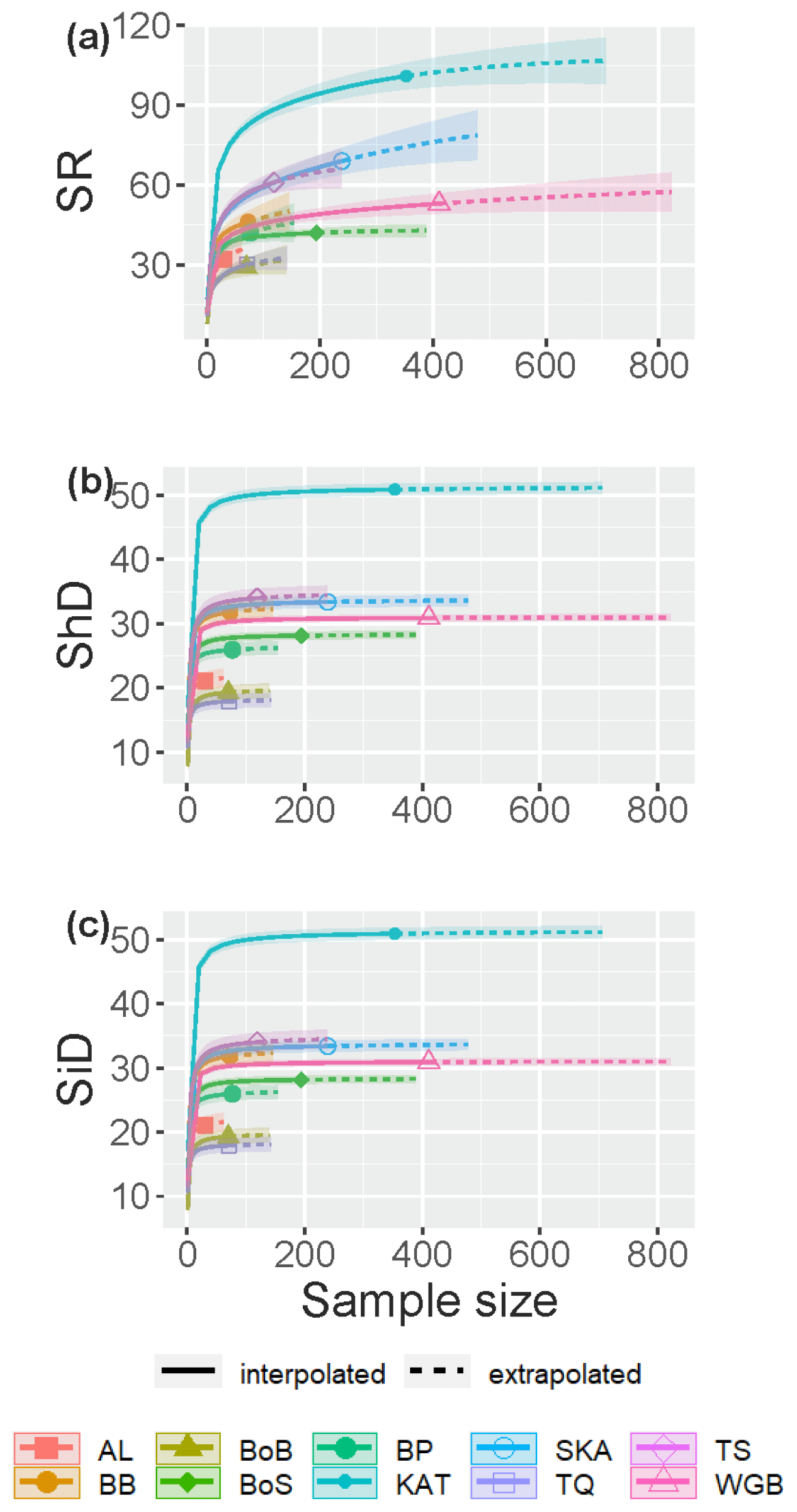
Figure 1 Sample-size-based species accumulation curves showing rarefaction/interpolation (solid curve segments) and extrapolation up to twice the actual sample size (dashed curve segments; Chao et al., 2020) with 95 % confidence intervals (shaded areas) for (a) species richness (SR), (b) Shannon diversity (the effective number of frequent species in the assemblage, ShD) and (c) Simpson diversity (the effective number of very frequent species in the assemblage, SiD) of fish in shallow coastal areas of the 10 assessed sub-basins. The intersection points between solid and dotted lines represent the observed values. Legend acronyms are AL: Åland Sea; BB: Bornholm Basin; BoB: Bothnian Bay; BoS: Bothnian Sea; BP: north Baltic Proper; KAT: Kattegat; SKA: Skagerrak; TQ: the Quark; TS: the Sound; and WGB: western Gotland Basin.

The SACs also visualize differences in IC between sub-basins. For the three most saline sub-basins, the Skagerrak, the Kattegat and the Sound, the SACs were still clearly increasing with increasing sample size even when extrapolating to double the actual sample size. Hence, the SR_est values for these sub-basins are more uncertain and more likely biased low than for sub-basins where the curve flattened, illustrating a more complete inventory, e.g. western Gotland Basin and the Bothnian Sea (Fig. 1a). The SR_est values, estimated based on extrapolation of the information in the fish incidence database, were similar to SR_obs if complementing the incidence data with records from the additional data sources (Table 2).

3.4 Shannon and Simpson diversities

Rarefaction and extrapolation SACs carried out for Shannon diversity (ShD) show that the effective number of frequently recorded fish species was quite well captured by the samplings in all statistically assessed sub-basins, illustrated by SACs with small remaining slopes at extrapolated higher sample size. As for SR_obs, ShD was highest in the Kattegat, while the remaining nine sub-basins clustered in two separate groups. The lowest ShD was noted for the Åland Sea, the Quark and Bothnian Bay (Fig. 1b, Table S5). The effective number of highly frequent species, i.e. Simpson diversity (SiD), was also well captured in all sub-basins, being highest in the Kattegat, while SiD in the remaining sub-basins clustered in four groups (Fig. 1c, Table S5).

3.5 Standardized and estimated species richness

To compare coastal fish SR, ShD and SiD across sub-basins, we estimated their standardized values against the minimum observed SC in any of the sub-basins. This represented a standardization to the SC of the Arkona Basin data (98.5 %; Tables 2 and S3). SR_std was ca. 3 times higher in the relatively more saline Kattegat (SR_std=78) compared to the least saline Bothnian Bay (SR_std=24), as also confirmed by comparing the respective SR_est values (Table 2). The differences were smaller for ShD and SiD. For example, based on SiD_std and SiD_est, the effective number of highly frequent species was ca. 2 times higher in coastal areas of the Kattegat compared to Bothnian Bay (Table S3). This implies, as also seen from the SACs (Fig. 1), that the frequent and most frequent fish species were captured quite well by the samplings for all sub-basins and that remaining uncertainties in differences across the salinity gradient are mostly due to uncertainty in the numbers of highly rare fish species. The estimated SR per sub-basin (SR_est, statistical extrapolation of the fish incidence data) was very similar to the total SR_obs when also including species records from additional data sources, with a mean ratio of 1.07 ± 0.03 (calculated based on data presented in Table 2).

3.6 Relationships of SR with salinity and temperature

Species richness increased with increasing mean water salinity, which explained 37 %–55 % of the variance in the data based on SR_obs, ShD_obs and SiD_obs. Using the standardized or estimated values, i.e. values corrected for sample size, resulted in stronger correlations, i.e. higher explained variance (40 %–77 %; Fig. 2a–c, Table S6). SR_obs, ShD_obs and SiD_obs were not correlated with mean water temperature, but, using the standardized and estimated values, correlations with temperature were also significant (explaining 48 %–77 % of the variance; Fig. 2d–f, Table S6). The slope estimates of the linear regressions differed more across observed, standardized and estimated values for SR than for ShD and SiD (Table S6). Adding temperature as an explanatory variable to the regressions with salinity did not improve the model in any case (all P>0.14).

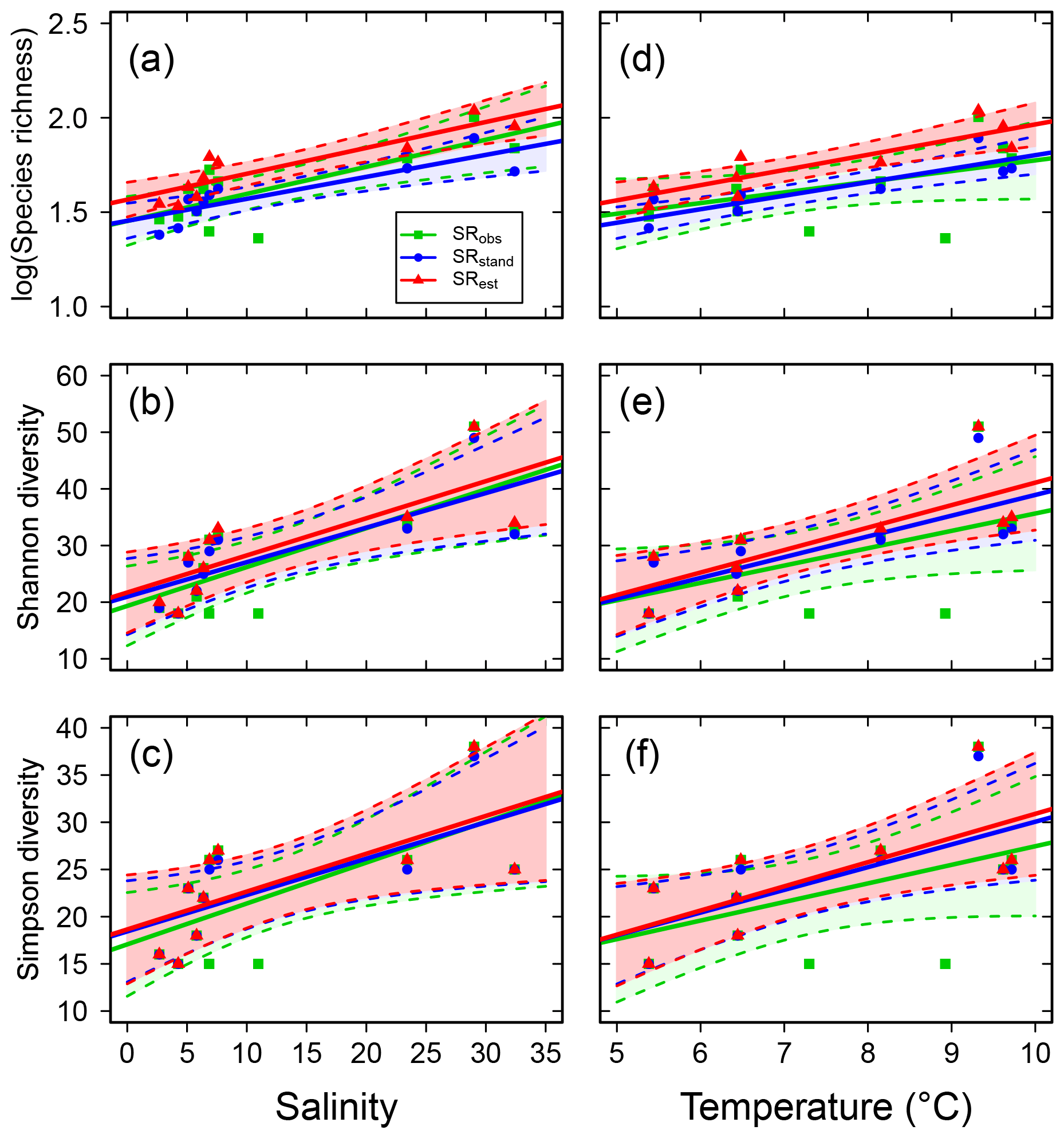
Figure 2 Fish species richness estimates in relation to mean salinity (left column) and mean water temperature (right column), with total species richness (log₁₀ transformed; a and d), Shannon diversity (effective number of frequent species; b and e) and Simpson diversity (effective number of highly frequent species; c and f). Each plot shows the observed, standardized and estimated values and, when significant (P<0.05), the linear regression lines (solid) and 95 % confidence intervals (shaded areas surrounded by dashed lines). Please note that data points (Table S7), lines and shaded confidence intervals are overlying each other within the panels in some cases. For regression equations and statistics, see Table 3.

Table 3 Simple linear regressions between salinity and SR for the different fish functional attributes (observed (obs), standardized (std) and estimated (est) SR) in Swedish shallow coastal areas. YJ(y) denotes that the response variable was Yeo–Johnson transformed (Yeo and Johnson, 2000). n.s. = not significant.

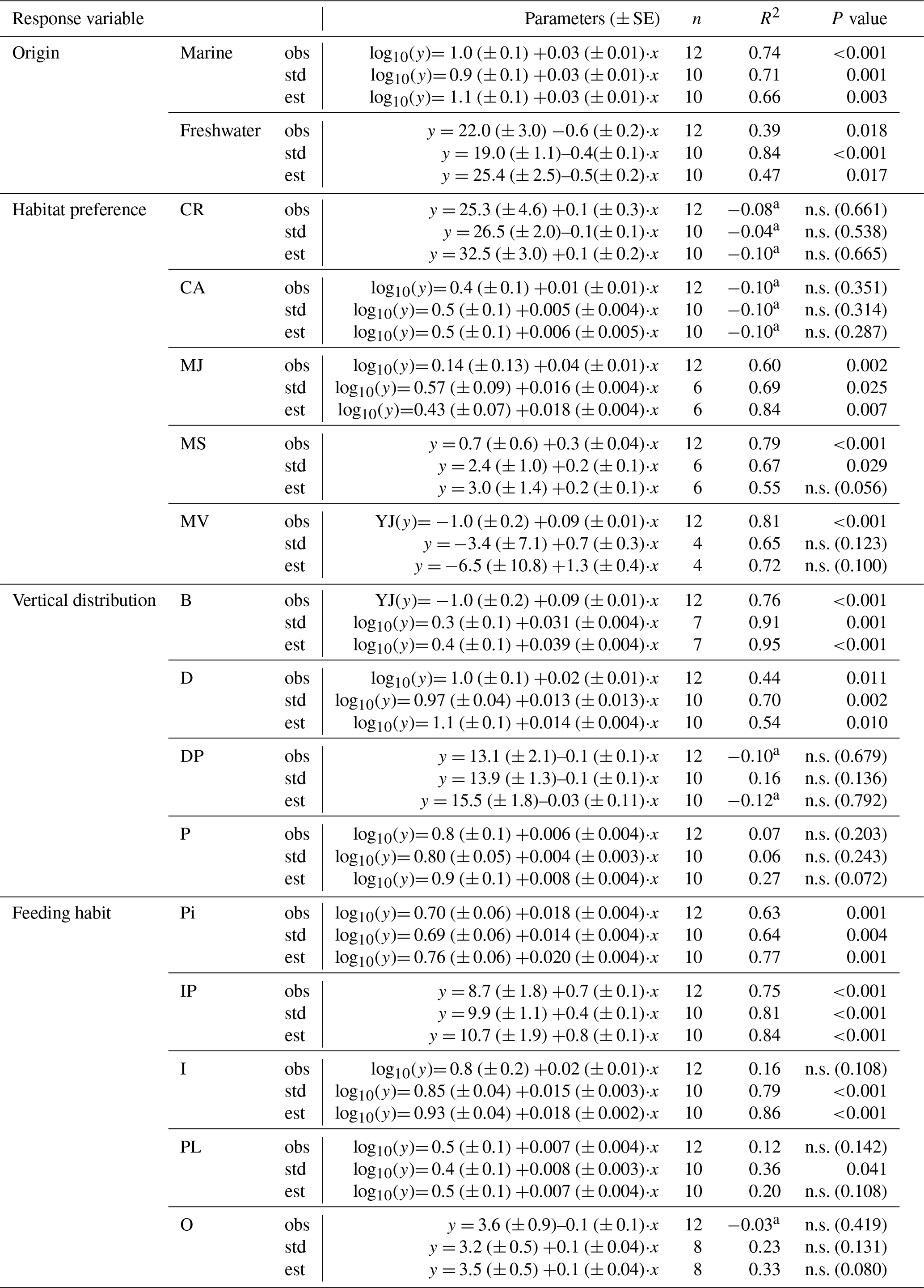
^a Adjusted R² can turn negative for multiple R² close to zero.

3.7 Fish functional attributes

Of the observed fish species, 74 % and 26 % were of marine and freshwater origin, respectively (based on the incidence data, i.e. SR_obs of 92 vs. 33 species; Table S3). In the most saline sub-basins, i.e. the Skagerrak and the Kattegat, the SR_std of marine fish species was 7 to 10 times higher than that of freshwater fish species. The SR_std values of marine vs. freshwater fish were rather similar in the central Baltic Sea, while in the northernmost and least saline sub-basins, i.e. Bothnian Sea, the Quark and Bothnian Bay, the SR_std of freshwater fish species exceeded the SR_std of marine fish species by 2 to 3 times. In total, the marine fish SR_std decreased by a factor of 8–11 along the salinity gradient, from 39 and 57 marine species (SR_std) in the Skagerrak and the Kattegat to 5 in Bothnian Bay. Freshwater fish SR_std increased by a factor of 2–4 along the same gradient (Fig. 3, Table S3). These distributional patterns of freshwater vs. marine fish species were also reflected by negative univariate correlations of freshwater SR (obs, std and est) with salinity and positive univariate correlations of marine SR with salinity (Fig. S1 in the Supplement, Table 3).

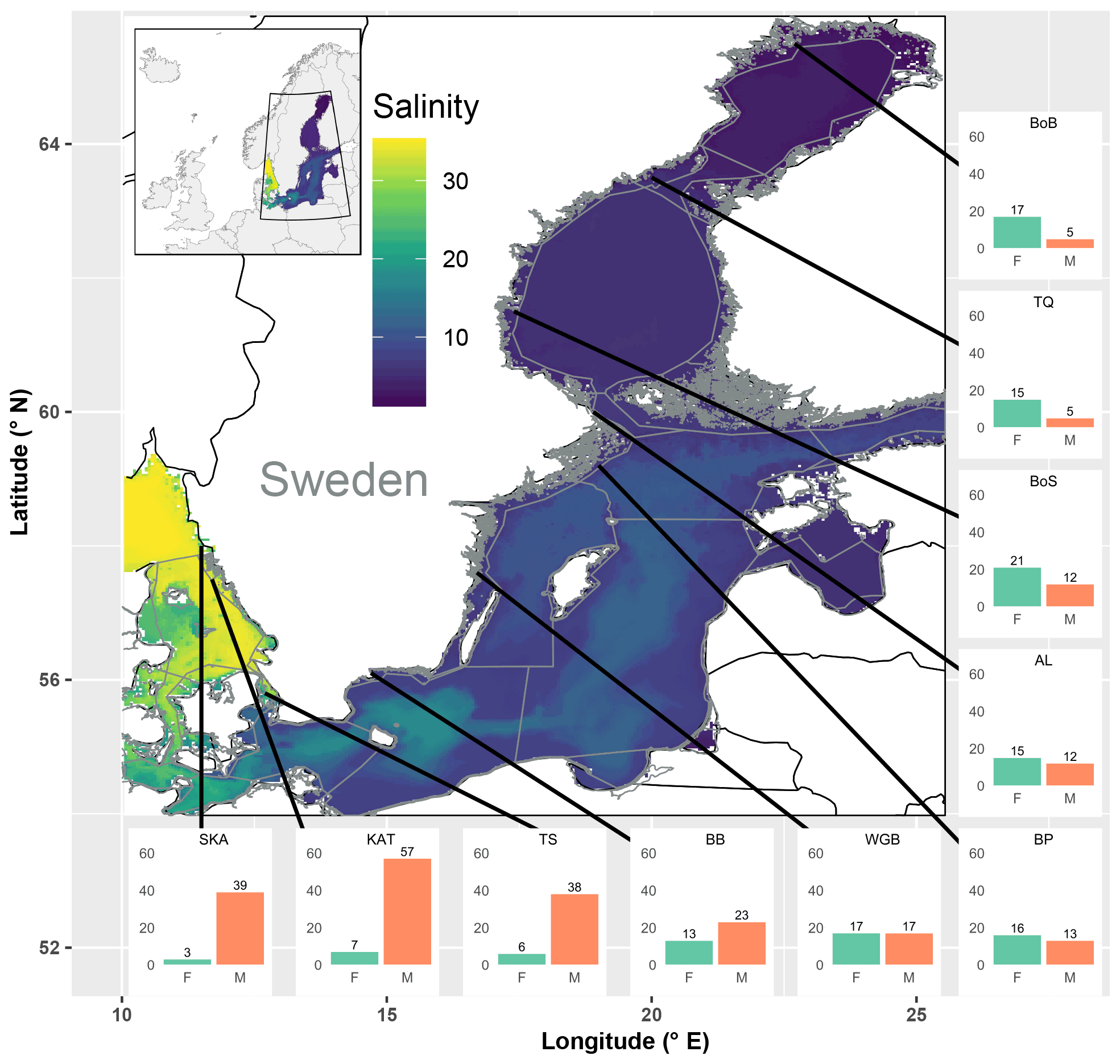
Figure 3 Map of the study area covering the Baltic Sea and the Skagerrak, colour-coded by mean salinity. Grey lines delineate sub-basins and shallow coastal areas. Bar plots show standardized fish species richness for shallow coastal areas in each of the 10 assessed sub-basins, separately for species of freshwater (F) and marine (M) origin. SR was standardized across sub-basins to similar sample coverage (Table S5). Black lines indicate the positions of the sub-basins, but the exact sampling sites were spread across the shallow areas of each of the sub-basins. SKA: Skagerrak; KAT: Kattegat; TS: the Sound; BB: Bornholm Basin; WGB: western Gotland Basin; BP: northern Baltic Proper; AL: Åland Sea; BoS: Bothnian Sea; TQ: the Quark; and BoB: Bothnian Bay.

Concerning habitat preference, half of the fish species in Swedish shallow coastal areas were classified as being coastal resident species (CR; based on the incidence database only, SR_obs: 63 species; Table S3). This group dominated coastal fish assemblages in all sub-basins, with CR SR_std of 19–30 across sub-basins (Fig. S2, Table S7), and was not linearly related to salinity (Fig. 4a, Table 3). A similar result was noted for catadromous or anadromous fish species, with SR_std of 2–6 across sub-basins and CA SR_std not related to salinity (Fig. 4b, S2, Tables 3, S7). In the more saline sub-basins, fish species classified as marine visitors or as marine juvenile or seasonal migrants contributed significant numbers to the SR_std, while these species groups did not exist or contributed only little to the SR_std in the Baltic Sea region (Fig. S2, Table S7). Reflecting this pattern, the SR of marine migrating or visiting fish species (i.e. MJ, MS and MV) was significantly positively related to salinity in most cases, with the strongest correlations for marine juvenile visitors (MJs; Fig. 4c–e, Table 3).

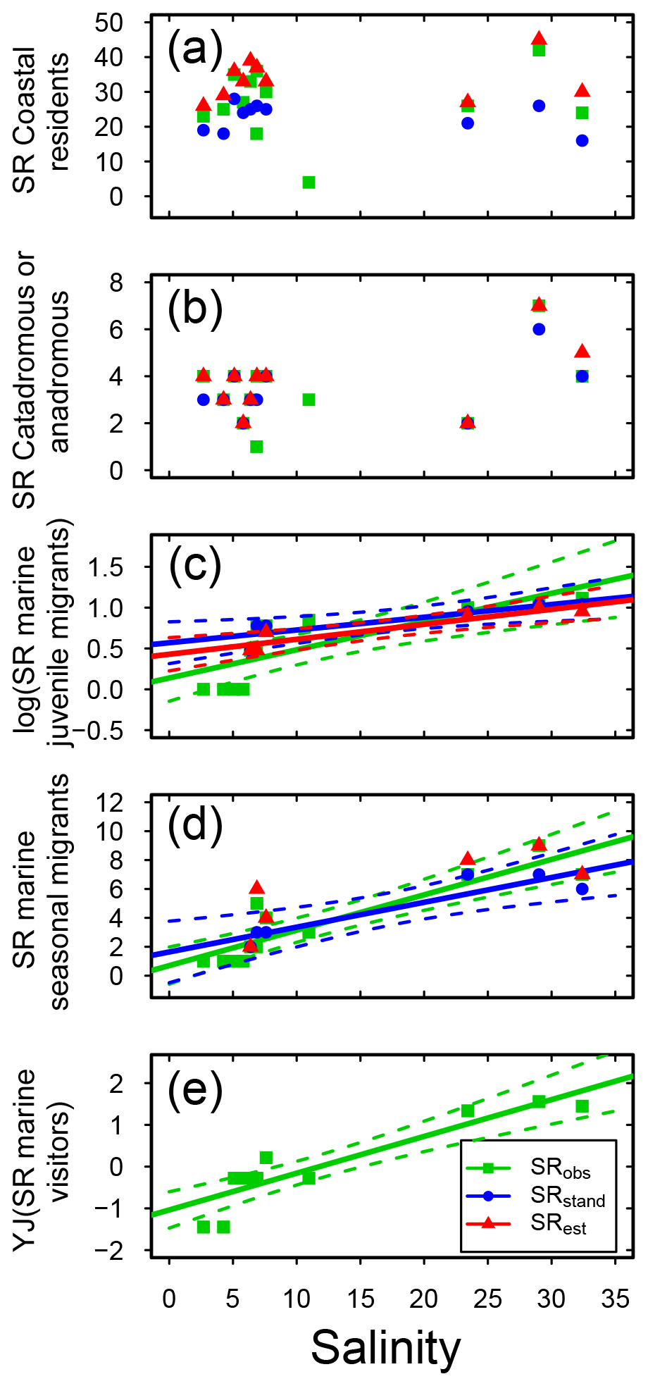
Figure 4 Fish species richness (SR) in relation to salinity in Swedish shallow coastal areas for different types of habitat preference, with (a) coastal residents, (b) catadromous or anadromous migrants, (c) marine juvenile migrants (log₁₀ transformed), (d) marine seasonal migrants, and (e) marine visitors (Yeo–Johnson transformed). Each plot shows the observed, standardized and estimated SR and, when significant (P<0.05), the linear regression lines (solid) and 95 % confidence intervals (shaded areas surrounded by dashed lines). Please note that data points (Table S7), lines and shaded confidence intervals are overlying each other within the panels in some cases. For regression equations and statistics see Table 3. For marine visitors (e), for clarity following transformation, only the observed SR is shown (no transformation was needed for the standardized and estimates values, and there were no significant relationships; Table 3).

Concerning vertical distribution, benthic fish species (B) were important contributors to SR_std in the sub-basins of higher salinity, but only a few or no fish species belonged to this group in the less saline sub-basins (Fig. S3; Table S7). A similar though less pronounced distribution pattern was also found for demersal fish species (D). Accordingly, the SR of these groups were positively related to salinity in all cases (i.e. for SR_obs, SR_std and SR_est; Fig. 5a, b, Table 3). The SR of demersal–pelagic (DP) fish species varied between sub-basins with a SR_std of 6–16 not related to salinity (Fig. 5c, Table 3). A similar picture was found for pelagic fish species (P), in which SR_std varied between 5 and 12 across sub-basins (Fig. S3, Table S7) and was not related to salinity (Fig. 5d, Table 3).

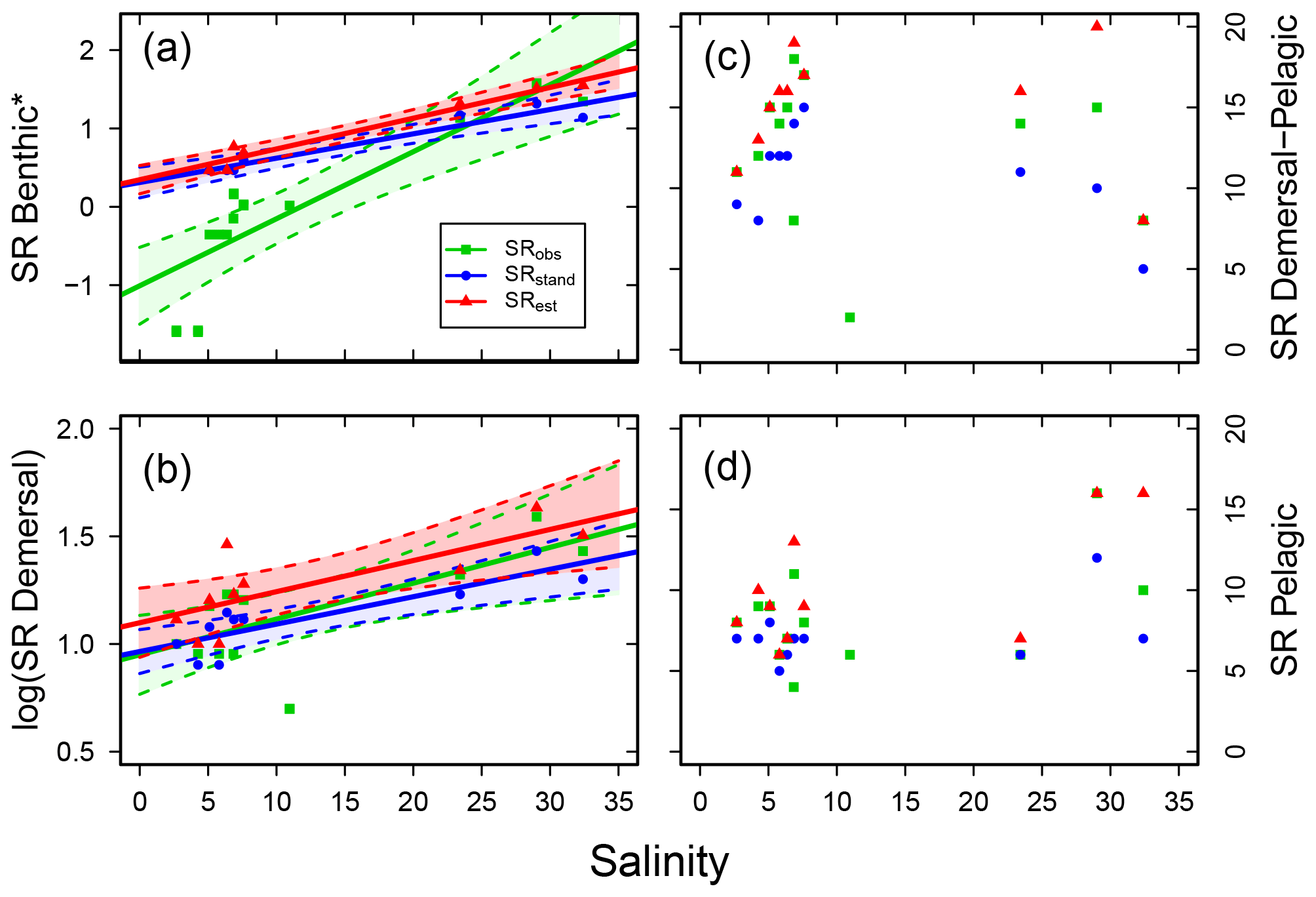
Figure 5 Fish species richness (SR) in relation to salinity in Swedish shallow coastal areas for different types of main vertical distribution, with (a) benthic (^*Yeo–Johnson transformed for SR_obs and log₁₀ transformed for SR_std and SR_est), (b) demersal (log₁₀ transformed), (c) demersal–pelagic and (d) pelagic fish species. Each plot shows the observed, standardized and estimated SR and, for cases with a significant linear relationship (P<0.05), also the regression line (solid) and 95 % confidence intervals (shaded areas surrounded by dashed lines). Please note that data points (Table S7), lines and shaded confidence intervals are overlying each other within the panels in some cases. For regression equations and statistics see Table 3.

The two most common feeding groups, across all sub-basins, were invertivore and piscivore (IP) species, as well as invertivores (I). The third-most represented feeding group was piscivores (Pi), followed by planktivores (PL) and omnivores (O) with lower and often similar SR_std (Fig. S4, Table S7). SR_std of Pi and IP increased with increasing salinity, and SR_std and SR_est of I increased with increasing salinity (Fig. S5, Table 3).

4 Discussion

Data from species censuses have been called “probably the most basic data in ecology” as they are widely useful, for example, to define species ranges and biodiversity patterns and support conservation efforts (Gaston and Blackburn, 2000). A limitation for the use of taxonomic inventory data for biodiversity purposes, however, is their completeness, i.e. the fraction of species in a given location that has been sampled (Mora et al., 2008). In this study, the coastal fish taxonomic inventory completeness (IC) varied between 77 % and 98 % for the 10 assessed sub-basins, exceeded 80 % in eight sub-basins, and averaged 86 % (Table 2). The comparatively low IC in the Skagerrak (77 %; Table 2) can be related to, in this context, a rather small sample size for a relatively high number of marine migrating and/or visiting species which are only more rarely present in this sub-basin and hence harder to detect during sampling (Fig. S2, Table S7). The average IC of 86 % in shallow Swedish coastal waters is high compared to an assessment of marine fish species census data worldwide, in which global IC averaged 79 %, indicating that ca. 21 % of fish species still remained to be described. Marine fish IC exceeded 80 % in less than 2 % of marine areas worldwide, with the highest IC of 92 % found for reef-associated species and the lowest of 56 % for bathydemersal species (Mora et al., 2008). Similarly, a global assessment published in 2012 concluded that ca. 77 % of marine fish were known.

The SR of frequent and very frequent species (i.e. Shannon and Simpson diversities, ShD and SiD) were well described by the sample sizes available to date in the assessed sub-basins, with calculated (“observed”) ShD and SiD being similar to both standardized and estimated values (when effects of differing sample sizes are considered; Table S5). This indicates that the remaining uncertainty in fish SR_obs is caused by a number of highly rare species, corroborated by a high sample coverage (SC) across sub-basins (Table 2). This is a typical pattern since well-known species are usually common and have large geographical ranges, whereas newly discovered species are usually (more) locally rare and geographically concentrated (Appeltans et al., 2012; Mora et al., 2008; Pimm et al., 2014). Specifically, in terms of species numbers and depending on the sub-basin, 1–37 statistically likely existing and highly rare fish species remained undetected in the samplings (Table 2, SR_est minus SR_obs). However, the high similarity between SR_est and total SR_obs (i.e. SR_obs based on incidence data plus species records from additional data sources; Table 2) suggests that the total observed species lists for fish in Swedish shallow coastal areas were close to complete for all assessed sub-basins, i.e. including the highly rare species undetected in the fish surveys (i.e. incidence database). This comparison between SR_est and total SR_obs also independently confirmed/validated that the SR values estimated based on the fish incidence database (SR_est) were realistic.

The most recent checklist of Baltic Sea macrospecies, i.e. containing fish species reported across Baltic countries at both shallow and deeper water depths but excluding the Skagerrak, contains 242 fish species (HELCOM, 2020). In our analyses of Swedish shallow coastal areas the total fish SR_obs amounted to 144 (i.e. SR_obs from incidence data plus additional data sources), also if the Skagerrak is excluded. Comparing the sample-size-corrected estimates of SR in coastal areas (SR_est) with the sub-basin-specific SR_obs of HELCOM (2020) suggests that ca. 50 %–90 % of all reported Baltic Sea fish species are found in Swedish shallow coastal areas (i.e. 100⋅SR${}_{\mathrm{est}}/$ SR_obs all countries and depths; Table 2).

Our study reinforces that SR_obs is strongly dependent on SC, as relatively rare species are more likely to be missed at lower sample size/sample coverage, and that comparisons of SR_obs in species assemblages without accounting for this effect can lead to biased or misleading conclusions (Chao and Chiu, 2016; Colwell and Coddington, 1994; Gotelli and Colwell, 2001; Hill, 1973; Menegotto and Rangel, 2018; Pimm et al., 2014). When sample sizes are not uniform among sites or over time, SR_obs values need to be corrected for SC before valid comparisons can be made. However, such methods have so far only rarely been used for coastal and estuarine fish assemblages (Waugh et al., 2019).

Besides the effects of sample size, SR and IC might to some extent also have been differentially influenced by differences in predominating sampling gear across sub-basins. Multi-mesh gill nets dominated in seven of the statistically assessed sub-basins, while trap nets and trawls dominated in the other three (Table S1). As one “sample” in each of these cases represents a different effort due to differences in gear selectivity and sampling approach, this strictly does not allow for direct comparisons (Bergström et al., 2013; Waugh et al., 2019). For example, at the Swedish west coast, gill nets typically sample a wider range of species than fyke nets, which are more selective towards demersal and demersal–pelagic species (Bergström et al., 2013). Merging data from multiple gear types into one analysis may have caused a certain bias in this regard. However, we argue that our approach was feasible given that the gear types used in the different sub-basins are optimized for the locally prevailing conditions, i.e. aiming to sample the existing assemblages as completely as possible (Bergström et al., 2013), as additional data from relevant trawl surveys were also included, and considering the long time horizon of data collection. Further supporting our approach, biodiversity metrics that were standardized against catch size revealed no consistent differences when comparing gill and fyke net samplings at the Swedish west coast (Bergström et al., 2013). Our assumption also appears justified given that SR_est was similar to SR_obs from incidence data plus species records from additional data sources (Table 2), giving confidence that the potentially introduced bias due to differing fishing gear and methods did not strongly influence the general patterns and results of this comparative and large-scale statistical analysis.

As anticipated based on earlier Baltic Sea studies on fish (e.g. Hiddink and Coleby, 2012; Ojaveer et al., 2010; Olsson et al., 2012) and other organism groups (e.g. Broman et al., 2019; Zettler et al., 2014), coastal fish SR was positively correlated with salinity (Fig. 2a, Table S6), with fish SR increasing ca. 3-fold together with the ca. 12-fold increase in salinity (Table 2). The clear predominance of marine species in the most saline sub-basins compared to freshwater species in the inner parts of the Baltic Sea (Fig. 3, Table S7) is in agreement with the fact that salinity functions as threshold or “ecological barrier” for the distribution of many freshwater and marine species (Olenin and Leppäkoski, 1999; Vuorinen et al., 2015). It also corroborates patterns reported earlier for fish SR_obs in three Baltic sub-basins (Hiddink and Coleby, 2012) and estuaries in general (Whitfield, 2015). The relatively small number of freshwater fish species incidences observed in the higher-salinity sub-basins in our study (Fig. 3) likely stems from sampling close to freshwater tributaries and reflects that many freshwater fish species can stand extended exposure to certain salinity levels (< ca. 9) and tolerate brief exposure to higher salinities (> ca. 15; Peterson and Meador, 1994).

While temperature did not significantly correlate with observed SR, ShD or SiD, it was positively correlated with the standardized and estimated values (Fig. 2d–f, Table S6), which may indicate a temperature effect on fish biodiversity. In previous studies, temperature has shown positive correlations with SR_obs in North Atlantic demersal and benthopelagic fish assemblages (Gislason et al., 2020), as well as with fish SR_obs in the coastal Norwegian Skagerrak (Lekve et al., 2002), and in estuaries worldwide (Vasconcelos et al., 2015), all being examples of the often found general pattern that broader-scale SR co-varies with climatic variables such as temperature (Currie et al., 2004). However, given the clear relationship between salinity and the incidences of freshwater vs. marine fish species across the studied sub-basins (Fig. 3), we consider the studied salinity gradient to represent a case to which the “physiological tolerance hypothesis” applies strongly, i.e. that SR in a particular area is limited by the number of species that can tolerate the local salinity conditions (Currie et al., 2004). In accordance, the regression models with salinity alone did not improve by adding temperature as an additional explanatory variable. This conclusion is in agreement with observations from estuaries that fish SR is influenced by the broader distributions and habitat preference patterns of marine and freshwater species that can colonize these areas (Vasconcelos et al., 2015).

Besides salinity and temperature, which show a pronounced gradient over the large spatial scale of our study (Table 1) and were identified as likely main drivers here (Fig. 2), fish SR might also be influenced by other factors, such as, for example, human pressures. The cumulative pressure from human activities in the Baltic Sea, combining factors such as fishing, eutrophication and hazardous substances, is generally higher in the southern and southwestern sub-basins. These sub-basins also show both relatively higher salinity and fish SR compared to, for example, the northernmost sub-basins with lower cumulative human pressure, salinity and fish SR (Tables 1, 2; Korpinen et al., 2012; HELCOM, 2018). Hence, no negative relationship between cumulative human pressure and fish SR is expected on the large spatial and temporal scales studied here. This does, however, not contradict that variation in levels of human pressures can have effects on fish concerning other aspects, such as population sizes or growth rates (Olsson, 2019; Bastardie et al., 2021; Reckermann et al., 2022), or could possibly affect SR on smaller spatial scales than those studied here. Evidently, since the rarefaction and extrapolation analyses that we used here are based on species incidence frequencies (Chao et al., 2020), the statistical results could potentially be influenced by human pressures that alter these frequencies even if fish SR in itself may not be affected. However, given that the rarefied and extrapolated SR (i.e. SR_std and SR_est) values are based on SC, in which rare species are not influential, these statistics are rather robust against such effects (unless there would be severe changes in the incidence frequencies of common species).

Another potential explanatory factor to consider is habitat complexity, related to, for example, diversity of substrate or habitat-forming macrophytes, which can promote higher aquatic biodiversity (Soukup et al., 2021). Differences in habitat complexity may play some role in the observed large-scale patterns in fish SR given that macroalgal SR increases with increasing salinity across the Baltic Sea, with a larger share of habitat-forming and perennial species in more marine waters (Middleboe et al., 1997; Schubert et al., 2011). Hence, a greater habitat complexity with increasing salinity may enhance fish SR, further reinforcing any salinity-induced distributional pattern.

In compiling data we have assumed that salinity changes have been minor during the time period from which samples were obtained compared to the pronounced spatial salinity gradient (observations over 17 to 47 years in the statistically assessed sub-basins, during 1975–2021; Table S2). According to monitoring data from the Baltic Sea, temporal changes in surface salinity varied between an increase of 3 psu in the Kattegat and a decrease of 1 psu in the Bothnian Sea during the past decades (1980–2015; Ammar et al., 2021), which can be considered small compared to the spatial salinity gradient ranging from 3 to 29. Considering temporal patterns in SR and community composition, it was earlier reported that the observed fish SR increased in the Kattegat, Arkona Basin and the central Baltic during 2001–2008 (Hiddink and Coleby, 2012) and that the observed SR of demersal fish increased in the Baltic Proper and the Bothnian Sea during ca. 1971–2013 (Törnroos et al., 2019). First-time observations of known fish species in sub-basins where they were not previously caught have been particularly related to increasing spring temperatures (+3–6 ^∘C during 1980–2015; Ammar et al., 2021). Such potential temporal patterns were not analysed in our study, in which we focused on large-scale spatial patterns and merged the fish incidence data across years to provide as accurate as possible SR estimates at the sub-basin scale.

Along with the changes in species, our study revealed changes in fish SR for different functional groups across the studied salinity gradient. As the functional groups represent differences among species groups in, for example, use of resources or level of mobility, these changes may also lead to differences in coastal ecosystem functioning across the different sub-basins (Elliott et al., 2007; Franco et al., 2008). Migrating fish species are typically of marine origin (here, marine juvenile migrants, marine seasonal migrants or marine visitors) and cannot tolerate low salinity, explaining their predominance at higher salinities (Fig. S2) and being in agreement with known patterns in European estuaries in general (Elliott and Dewailly, 1995; Franco et al., 2008). This pattern, with marine open-sea fish species periodically using coastal areas, may be related to enhanced prey availability, hiding places, and the typically more turbid waters providing protection from predators (Franco et al., 2008). Moreover, the higher SR of migratory fish at higher salinity is likely relevant for the ecological connectivity between ecosystems, i.e. by transport of local “coastal” production to the open sea and vice versa (Franco et al., 2008). It also emphasizes the important role of coastal areas as nursery grounds, migration routes and refuge areas for marine fish species (Elliott et al., 2007). Connectivity is also maintained in the less saline sub-basins, though the concerned functional groups are represented by only a few species (Fig. S2; Berkström et al., 2021).

Further, benthic and demersal fish SR decreased with decreasing salinity (Fig. 5a, b, Table 3), corroborating a previously documented decrease in demersal fish SR_obs from the saline Kattegat to the less saline northern Baltic Proper (Pecuchet et al., 2016) and in accordance with the high benthic preference of marine fish species in European estuaries (Elliott and Dewailly, 1995; Franco et al., 2008). This pattern further corresponds with the observed SR of benthic meio- and macrofauna, which are a dominating prey for benthic and demersal fish, also decreasing with decreasing salinity in the Baltic Sea (Broman et al., 2019; Zettler et al., 2014). Taken together, these patterns suggest that benthic–pelagic coupling through fish predation likely involves a lower number of species links, or functional redundancy, towards lower-salinity sub-basins. Concerning feeding habits, the general composition of feeding guilds noted in the higher-salinity sub-basins was similar to that reported on a larger European scale (Elliott and Dewailly, 1995). Also, the higher piscivorous fish SR in the more saline sub-basins (Fig. S5e) and the low omnivorous fish SR which was unrelated to salinity (Fig. S5c) were in agreement with findings from European estuaries (Franco et al., 2008). In summary, the identified differences in functional traits of fish along the salinity gradient were largely related to the respective changes in the predominating fish origin, i.e. freshwater vs. marine species.

5 Conclusions

Since fish SR and a number of functional attributes changed along the salinity gradient, respective changes in the coastal fish communities may be foreseen if climate change further alters salinity conditions in the Baltic Sea. While the confidence in future salinity projections remains low (HELCOM, 2021), recent ensemble simulations estimate that the two main drivers of climate-related changes in salinity in the Baltic Sea region, increasing river runoff (leading to lower salinity) and sea level rise (leading to higher salinity), approximately compensate for each other and may result in no net salinity changes (Meier et al., 2022). Mean (depth-integrated) observed Baltic Sea salinity did not change during 1982–2016; however, vertical changes were observed with freshening trends of the upper layer down to 40–50 m depth in most sub-basins and increasing salinity below the halocline in the deep layer of some sub-basins (Liblik and Lips, 2019). Hence, if not considering potential phenotypical acclimation or genetic adaptation, an upper-layer freshening would, based on the results from this and earlier studies (e.g. Hiddink and Coleby, 2012; MacKenzie et al., 2007; Pecuchet et al., 2016), likely lead to reduced native fish SR in shallow coastal areas, where more and more marine species are excluded. Further, successful recovery of marine overfished species may become less probable, while certain freshwater fish species may be favoured (MacKenzie et al., 2007; Peterson and Meador, 1994). Indeed, marine fish species were negatively affected by a period of freshened conditions in the Baltic Sea during the ca. 1970s–1990s (Ojaveer and Kalejs, 2005). Benthic fish species, being mostly of marine origin, may be especially vulnerable to freshening in the inner Baltic Sea (i.e. Arkona Basin and inwards) where their proportion in the fish assemblage is already relatively low to date.

Besides salinity changes, fish SR and distribution may also be influenced by other climate-change-related processes, including warming and resulting higher deep-water oxygen consumption rates, or changes in the Baltic Sea circulation (HELCOM, 2021; MacKenzie et al., 2007). Increasing water temperatures have already been linked to increased observed fish SR in the adjacent North Sea (Hiddink and Ter Hofstede, 2008) and in the Kattegat (Hiddink and Coleby, 2012). Further ecosystem-based assessments are needed to obtain realistic predictions of the net effect of such ongoing environmental changes on future fish SR and community composition and on how they may interact with human activities such as fishing patterns, as well as with conservation needs for biodiversity management.