the Creative Commons Attribution 4.0 License.
the Creative Commons Attribution 4.0 License.
 | 07 Jul 2022
Contrasting vertical distributions of recent planktic foraminifera off Indonesia during the southeast monsoon: implications for paleoceanographic reconstructions
Hui-Yu Wang
Jeroen Groeneveld
Mahyar Mohtadi
Planktic foraminifera are widely used in paleoceanographic and paleoclimatic studies. The accuracy of such reconstructions depends on our understanding of the organisms' ecology. Here we report on field observations of planktic foraminiferal abundances (>150 µm) from five depth intervals between 0–500 m water depth at 37 sites in the eastern tropical Indian Ocean. The total planktic foraminiferal assemblage here comprises 29 morphospecies, with 11 morphospecies accounting for 90 % of the total assemblage. Both species composition and dominance in the net samples are broadly consistent with the published data from the corresponding surface sediments.
The abundance and vertical distribution of planktic foraminifera are low offshore western Sumatra and increase towards offshore southern Java and the Lesser Sunda Islands (LSI). Average living depth of Trilobatus trilobus, Globigerinoides ruber, and Globigerina bulloides increases eastward, while that of Neogloboquadrina dutertrei, Pulleniatina obliquiloculata, and Globorotalia menardii remains constant. We interpret the overall zonal and vertical distribution patterns in planktic foraminiferal abundances as a response to the contrasting upper-water-column conditions during the southeast monsoon, i.e., oligotrophic and stratified offshore Sumatra (non-upwelling) vs. eutrophic and well mixed offshore Java–LSI (upwelling). Overall, the inferred habitat depths of selected planktic foraminifera species show a good agreement with those from sediment trap samples and from surface sediments off Sumatra, but not with those from surface sediments off Java–LSI. The discrepancy might stem from the different temporal coverage of these sample types. Our findings highlight the need to consider how foraminiferal assemblages and ecology vary on shorter timescales, i.e., from “snapshots” of the water column captured by a plankton net to seasonal and interannual variability as recorded in sediment traps, and how these changes are transferred and preserved in deep-sea sediments.
- Article
(11689 KB) - Full-text XML
-
Supplement
(125 KB) - BibTeX
- EndNote


Planktic foraminifera's diversity, community composition, population dynamics, and their shell chemistry are sensitive to hydrographic parameters (e.g., temperature, salinity, food availability) of the upper ocean (Bemis et al., 1998; Fairbanks et al., 1980; Katz et al., 2010). Consequently, their assemblage composition and the geochemical signature of their shells are routinely used to reconstruct past ocean conditions (e.g., Ding et al., 2006, 2013; Mohtadi et al., 2017; Steinke et al., 2014).
Since the early observations from Murray (1897), many studies have evaluated the relationship between seawater temperature and planktic foraminiferal distribution and found increasing dominance of cold species with increasing latitudes (Bé and Hamlin, 1967; Eguchi et al., 1999). This relationship with seawater temperature allowed the development of the first comprehensive mapping of past sea surface temperature (SST) (CLIMAP Project Members, 1976). Subsequent assemblage studies have attempted to improve the accuracy of past sea surface temperature reconstruction via the transfer function approach (e.g., Imbrie and Kipp, 1971; Ortiz and Mix, 1997). Although seawater temperature has a large influence on the global distribution of planktic foraminifera (Kucera, 2007, 2009), other parameters such as salinity, oxygen content, food availability, turbidity, and upwelling intensity can also exert a strong control on the abundance, community structure, and vertical distribution of planktic foraminifera at regional scales (Anderson et al., 1979; Davis et al., 2021; Field, 2004; Lessa et al., 2020; Rebotim et al., 2017; Schiebel and Hemleben, 2017; Tolderlund and Bé, 1971).
In the last decades, geochemical proxies using the calcite tests of foraminifera (e.g., isotope δ18O and trace elements such as ratios) have become a powerful tool for the reconstruction of past ocean conditions (Katz et al., 2010; Lea, 2014; Schiebel et al., 2018). The robustness of paleoclimate reconstructions derived from foraminiferal calcite proxies is as good as our understanding of the multiple fields that planktic foraminiferal biology encompasses (Schiebel et al., 2018). For example, reconstructing past changes in the water column structure using multiple planktic foraminiferal species (e.g., surface vs. deep dweller) requires understanding of the ecology of the selected species, such as seasonality, habitat depth, and food requirements (Kemle-von Mücke and Oberhänsli, 1999; Kucera, 2007; Marchant et al., 2004; Schiebel et al., 2017). One common way of inferring planktic foraminifera habitat depth is by using the calcification depth, obtained by comparing the reconstructed parameters (typically SST) from surface sediments with instrumental data or climatological products (e.g., World Ocean Atlas) (Groeneveld and Chiessi, 2011; Hollstein et al., 2017; Mohtadi et al., 2011; Steinke et al., 2014; Tapia et al., 2015). In this approach, calcification depth is defined as the water depth at which the reconstructed temperature or seawater δ18O value shows the closest match with the instrumental data or climatological product. However, calcification depth does not necessarily coincide with the inferred habitat depth where the organisms are observed during sampling. Also, this approach may be associated with uncertainties arising from a myriad of processes during the settling, deposition, and burial that may lead to varying degrees of proxy signal alteration (Regenberg et al., 2014). Furthermore, additional uncertainty stems from the selected proxy calibrations and the instrumental database used for comparison with the proxy. “Snapshots” from the water column where planktic foraminifera dwell thus provide additional information to improve proxy understanding.
The marginal seas of the Indonesian Archipelago are of great climatic importance. Here, the Indonesian Throughflow (ITF) connects the upper water masses of the Pacific and Indian oceans, exerting a strong effect on the salinity and heat exchange between these basins (Gordon and Fine, 1996; Gordon, 2005; Tillinger, 2011). This feature has fueled the scientific interest to better understand the role that heat exchange plays in climatic modulation on several timescales (Smith et al., 2020; Sprintall and Révelard, 2014). Consequently, a growing number of oceanographic reconstructions based on foraminiferal calcite have been published over the last decade to shed light on the changes in the regional oceanographic processes and climate (Dang et al., 2020; Ding et al., 2013; Fan et al., 2018; Karas et al., 2011; Mohtadi et al., 2014, 2017; Pang et al., 2021; Steinke et al., 2014; Wang et al., 2018). However, our understanding of the ecology of planktic foraminifera in this region, especially their vertical distribution, relies largely on indirect inferences based on surface sediments and sediment trap samples (Ding et al., 2006; Mohtadi et al., 2007, 2009, 2011). Thus far there is only one field observation that is focused on the standing stock of planktic foraminifera in surface ocean sampled using a plankton net (Ujiié, 1968), but this study did not investigate the vertical distribution of planktic foraminifera in the water column. To fill this gap, here we present depth-stratified (0–500 m) plankton net data from the Indonesian marginal seas off Sumatra, Java, and the Lesser Sunda Islands (LSI) (Fig. 1). The main goal of this study is to shed light on the spatial distribution of planktic foraminifera during the southeast (SE) monsoon, on the relationship between foraminiferal abundance and environmental parameters, and on how these findings compare with sediment trap and core top assemblage data to further improve our understanding of foraminifera-based proxy reconstructions in this region.

Figure 1(a) Distribution of the in situ sea surface temperature in the study area during PABESIA cruise on board R/V Sonne in August 2005 (Hebbeln and cruise participants, 2006). The study area was divided into seven land–sea transects (numbered rectangles). The stations are divided into plankton net (white circles) and water (red diamonds). The locations of the sediment trap (Mohtadi et al., 2009) and surface sediments (Mohtadi et al., 2007) are indicated by the triangle and squares, respectively. Upper-ocean chlorophyll a (chl a) (retrieved from https://oceancolor.gsfc.nasa.gov, last access: 8 November 2021) during (b) January (non-monsoon) and (c) August (SE monsoon) 2005, i.e., the sampling period. Temperature map was created with the Ocean Data View 5.2.1 (Schlitzer, 2021).
Study area
Modern oceanography off Indonesia is strongly modulated by seasonal monsoons. During the SE monsoon from April to October, the southeasterly winds from Australia induce Ekman pumping that generates upwelling along the coast of southern Sumatra, Java, and the LSI. The peak of upwelling-favorable winds occurs at the southernmost coast of Sumatra ( E) during July–August, but the upwelling center moves northwestward, reaching as far as 100∘ E and 2∘ S in October (Susanto et al., 2001). Seasonal upwelling results in increased chlorophyll a concentrations and reduced thickness of the depth of the mixed layer (< 20 m) south of S (Fig. 1, Table A1 in the Appendix). Furthermore, seasonal upwelling leads to a ∼2 ∘C decrease in SST in comparison to the non-upwelling season and a contrast in SST of ∼3 ∘C between the northern and southern parts of the study area. During the northwest (NW) monsoon from late October to early April, the wind direction is reversed, resulting in downwelling, lower chlorophyll a concentrations, thicker mixed layer, higher SST south of S, and a more uniform SST distribution offshore southern Sumatra, Java, and the LSI (Muskananfola et al., 2021; Qu et al., 2005; Susanto et al., 2001, 2006). At the interannual timescale, the SST variability offshore southern Sumatra, Java, and the LSI can be larger than 4 ∘C, showing the influence of climatic modes such as El Niño–Southern Oscillation (ENSO) or the Indian Ocean Dipole (IOD) (Qu et al., 2005). During years of the El Niño (La Niña) phase of the ENSO and the positive (negative) phase of the IOD, intensified (weakened) southeasterly winds result in stronger (weaker) coastal upwelling, leading to abnormally low (high) SSTs offshore southern Sumatra and Java (Du and Zhang, 2015; Mohtadi et al., 2011; Qu et al., 2005).
Multinet samples were collected between August and September 2005 during R/V Sonne cruise SO-184 (Hebbeln and cruise participants, 2006). The 47 sampling sites are grouped into seven land–sea transects off Sumatra (n=4), Java (n=2), and the LSI (n=1) (Fig. 1; details in Table A1).
2.1 Collection of hydrographic data and foraminiferal samples
The characterization of the physicochemical properties of the water column (i.e., temperature, salinity, nutrients, oxygen, and in situ chlorophyll a) was obtained from CTD (conductivity–temperature–depth) and water samples collected using a rosette water sampler equipped with 24 Niskin bottles (10 L volume each) and a Seabird SBE911 probe (Hebbeln and cruise participants, 2006) across 45 water stations (see Table A1). These hydrographic data are available in the cruise report of SO-184 (Hebbeln and cruise participants, 2006). Briefly, the dissolved oxygen was determined using an automated titrator (TitroLine alpha), which is controlled by a redox electrode and a color agent (starch solution), on a self-constructed titration board for ship cruises according to the World Ocean Circulation Experiment (WOCE) protocol (Hebbeln and cruise participants, 2006). Chlorophyll a measurements were performed using a SFM25 spectrofluorometer (KONTRON). The measurements were done with 1 cm cuvettes at a 435 nm excitation wavelength and a 667 nm emission wavelength (Hebbeln and cruise participants, 2006).
The plankton samples (n=37; Table A1) were obtained using a MultiNet sampler (Hydro-Bios, Kiel, Germany). The gear is comprised of five individual 64 µm nets with an opening of 0.25 m2. The nets were lowered to a water depth of 500 m and vertically towed with a maximum winch speed of 0.2 m s−1 along five depth intervals of 500 to 200, 200 to 100, 100 to 50, 50 to 25, and 25 to 0 m depth. At the end of each depth interval the MultiNet sampler was stopped to open the next net, automatically closing the previous net. Once on board the samples were poisoned with 1 mL saturated HgCl solution and stored at 4 ∘C (Hebbeln and cruise participants, 2006). The volume of water passed through the net opening was calculated as the product of the height of the towed intervals and the area of the net opening.
2.2 Foraminiferal identification and census count
The taxonomic identification of the planktic foraminifera was based on Parker (1962), Kennett and Srinivasan (1983), and Hemleben et al. (1989). We used the same taxonomic approach as in previous studies based on surface sediments (Mohtadi et al., 2007) and a sediment trap (Mohtadi et al., 2009, 2011). The only exceptions are for Globigerinoides elongatus and Trilobatus trilobus as the names of these species have been updated recently by Aurahs et al. (2009) and Spezzaferi et al. (2015), respectively. Here the species Globigerinoides ruber (white) can occur in two morphotypes (Mohtadi et al., 2009, 2011), namely G. ruber sensu stricto (s.s.) and sensu lato (s.l.). As G. ruber (s.l.) is now identified as a separate species, Globigerinoides elongatus (Aurahs et al., 2009), we have included this distinction. The distinction was done according to the approach of Wang (2000); specimens with spherical chambers sitting on the previous suture and high arched primary aperture were classified as G. ruber (white). Meanwhile, more compressed organisms with subspherical chambers and low arched primary aperture were classified as G. elongatus. In the case of the genus Trilobatus, we integrated the sacculifer morphotype, i.e., individuals with a sac-like final chamber, into the counts of T. trilobus (individuals with a regular, globular terminal chamber). The distinction of Neogloboquadrina dutertrei from Neogloboquadrina incompta was made according to the approach of Mohtadi et al. (2009), based on the presence of an umbilical tooth and the occurrence of more than four chambers per whorl (Parker, 1962). The samples were separated into four size classes (>500, 500–355, 355–250, and 250–150 µm) and stored in foraminiferal microslides. Here we report the foraminiferal abundances >150 µm as individuals per volume of seawater passing through the opening of the net (individuals m−3).
Vertical habitat preferences were estimated using the total abundance of each species in each vertical profile. As we did not discriminate between living and dead specimens, this approach may have led to an overestimation of the habitat depth, for instance when specimens were found in deep nets. Therefore, we refrain from interpreting individual multinet deployments, which may be prone to the aforementioned bias. Instead, we base our interpretations on the median value of transects, each consisting of at least three multinet deployments. The proportion of dead specimens, if any, likely varies across stations; thus averaging over stations yields estimates that are less prone to single-site bias. This approach might also mitigate potential biases caused by patchy occurrences of planktic foraminifera in the water column, in both lateral and vertical directions (Meilland et al., 2019). To facilitate comparison with previous studies and to avoid bias due to different sampling strategies, we used average living depth (ALD) (Jorissen et al., 1995) to discuss the vertical habitat of planktic foraminifera. ALD is defined as
where ni is the number of specimens in the interval i of a particular species, Di is the midpoint of the sampled interval i, and N is the total number of individuals for all the depth levels of that particular species. For the calculation of the ALD, we followed the approach suggested by Rebotim et al. (2017) by considering only stations with at least five individuals of a given species.
The 95 % confidence interval of the species ALD for the upwelling vs. non-upwelling region (Table 1) was estimated using non-parametric randomization tests, i.e., bootstrap (Manly, 1997), as the distributions of ALDs of either region do not meet normal distributions required for parametric tests due to small sample sizes. The upwelling region consists of transects 5–7, while the non-upwelling region consists of transects 1–3. We permuted the ALDs of each species for the upwelling and non-upwelling region, respectively, simulating the differences in mean ALDs between these permuted sites with 999 replicates. We then sorted the sequence of 999 differences in mean ALDs, which approximated all possible outcomes of the lack of differences in mean ALDs between upwelling vs. non-upwelling sites. We determined the probability of the observed between-region difference in mean ALDs as one quantile of the observed estimate in the sorted sequence. The probability (P value) <0.05 represents significant differences in mean ALDs between regions. Statistical analysis was performed in the R language (R core Team, 2020; code available upon request).
Table 1The 95 % confidence interval of the habitat depth of six species of planktic foraminifera in upwelling vs. non-upwelling regions. The upwelling region consists of transects 5–7, while the non-upwelling region consists of transects 1–3. Details of the calculation are described in the “Materials and methods” section.
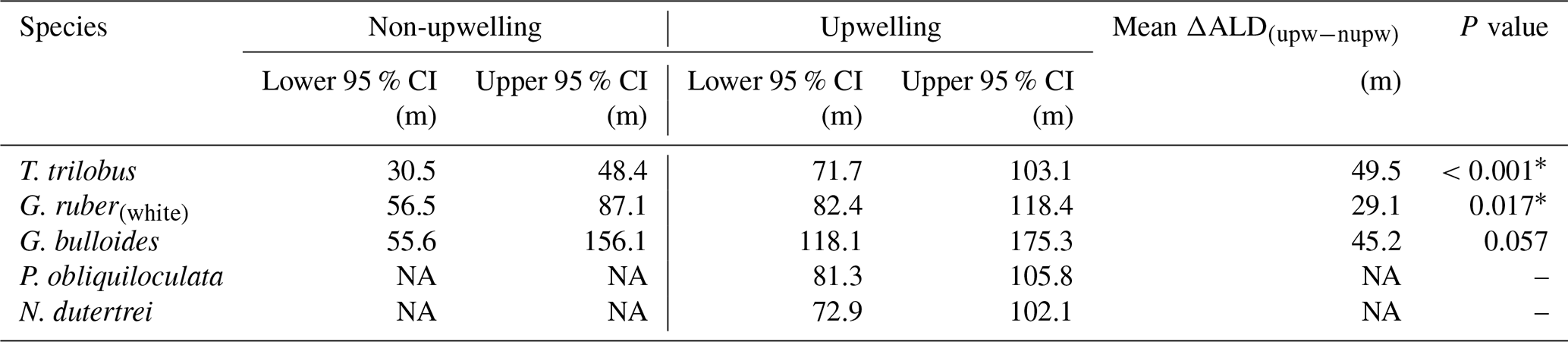
∗ Difference in ALD for the two regions is statistically significant. Abbreviations: CI for confidence interval, ALD for average living depth, upw – nupw for upwelling minus non-upwelling, NA for no data available.
3.1 Hydrological conditions
Across the sampled depths (0–500 m) of the plankton nets, the water temperature ranges from ∼8 to ∼30 ∘C, the salinity from 33.5 to 35.1, the in situ chl a from ∼0.2 to ∼0.7 mg m−3, and the oxygen concentration from 1.2–∼5 mL L−1 (Fig. 2a–d). Sea surface temperature shows a strong zonal contrast, with colder conditions off Java–LSI and warmer conditions off Sumatra (Fig. 2a). This zonal pattern remains across all the sampled depths from the surface to a water depth of 500 m (Fig. A1 in the Appendix). Similarly, salinity also shows a strong zonal contrast as fresher conditions dominate the upper 50 m of the water column off Sumatra, while more saline conditions dominate the upper ocean off Java (<50 m) (Fig. 2b). This pattern reverses at depths >50 m, with more saline conditions off Sumatra than Java and the LSI.
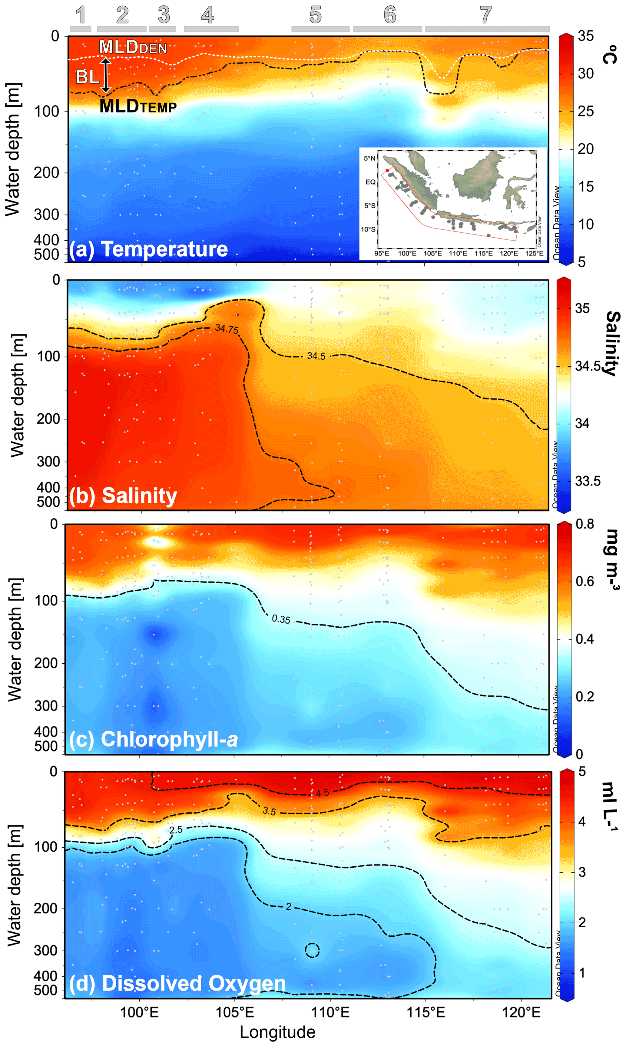
Figure 2Cross-sections of (a) water temperature, (b) salinity, (c) chl a, and (d) oxygen content of the upper 500 m of the water column during the sampling period. Location of the stations comprising the cross-section are depicted in the inset of (a). Thermal mixed-layer depth (MLDTEMP), density mixed-layer depth (MLDDEN), and barrier layer (BL) are marked in (a). Numbers and horizontal lines on top show each transect (1 to 7). Visualization is based on Ocean Data View 5.2.1 (Schlitzer, 2021).
In situ chl a for 0–25 m water depth is on average ∼0.65 mg m−3, with no zonal patterns across the study area (Table A1 and Fig. 2c). Lower-than-average chl a values can be found at two oceanic stations from transect 3 off Sumatra, that is, sites GeoB10003 (0.28 mg m−3) and GeoB10007 (0.34 mg m−3) (Table A1). Despite the absence of a zonal divide in surface chl a, at depths >50 m the vertical distribution differs between Sumatra and further east ( E; Fig. 2c). Off Sumatra ( E), chl a is mainly restricted to the upper 100 m of the water column, while high chl a values >0.3 mg m−3 (>105∘ E) can reach as deep as 500 m at the easternmost study area, i.e., transect 7 around Sumba Island (Fig. 2c). The distribution of oxygen content across the water column matches the distribution of in situ chl a; i.e., high dissolved oxygen concentrations (>2 mL L−1) are restricted to the upper 100 m of the water column off Sumatra, while high dissolved oxygen concentrations off Java and particularly around Sumba (transect 7) can reach as deep as 500 m (Fig. 2d).
The thermal mixed-layer depth (MLDTEMP) for this region, defined as the depth where the temperature is >0.8 ∘C colder than the SST (Kara et al., 2000; Qu et al., 2005), roughly marks the top of the thermocline depth and ranges from ∼13 to ∼91 m (Table A1 and Fig. 2a). We note that a different approach in defining mixed-layer depth (e.g., Boyer Montégut et al., 2004, for global ocean), would result in different thickness of the mixed layer, but this does not change the spatial pattern that is the focus of the discussion here. The MLDTEMP varies zonally; off Sumatra the MLDTEMP (∼70 m) is on average twice the thickness of that off Java–LSI (∼33 m) (see Table A1). The barrier layer separates the well-mixed upper ocean from the thermocline. Here, the barrier layer is defined as the MLDTEMP minus the mixed-layer depth calculated using density, namely MLDDEN (Qu and Meyers, 2005). It ranges between 0 and ∼72 m thickness and follows a similar spatial distribution as the MLDTEMP, with an average thickness of ∼38 m off Sumatra and ∼3 m off Java–LSI (Table A1). The upper-water-column stratification, SI0–200, is defined as the temperature difference between the sea surface and 200 m (Somavilla et al., 2017). The SI0–200 values are higher off Sumatra than off Java and the LSI, indicating a more stratified upper water column off Sumatra (Table A1). These observations suggest two contrasting hydrological conditions in the study area, with strong (weak) water column stratification, thick (thin) mixed layer and barrier layer, and low (high) subsurface water entrainment towards the surface off Sumatra (off Java–LSI), in agreement with the observed geographical extension of the coastal upwelling (Fig. 1c) during the SE monsoon (Susanto and Marra, 2005; Susanto et al., 2001).
Multivariate analysis (non-metric multidimensional scaling) performed on the in situ hydrographic data obtained during the cruise provides further evidence that the study area consists of three hydrologically distinct regions (Fig. 3), constituting transects 1–3, 4, and 5–7, respectively. The cluster off Java and the LSI that encompasses transects 5 to 7 is characterized by lower SST (<29 ∘C), saltier surface ocean, shallow mixed layer, and chl a with a larger vertical dispersion, i.e., conditions typical of seasonal upwelling during the southeast monsoon. Meanwhile, the cluster off Sumatra that encompasses transects 1 to 3 is characterized by higher SST (>29 ∘C), fresher surface ocean, deep mixed layer, and chl a with low vertical dispersion. A third cluster consists solely of transect 4, which reflects transitional conditions as here we can observe a large dispersion in the values of the parameters analyzed (see Table A1), and its location coincides with the northernmost extent of upwelling-favorable winds (see Sect. 1.1). The multivariate analysis performed on hydrographic data separates the sites into two main groups, i.e., transects 1–3 in the non-upwelling sector and transects 5–7 in the upwelling sector.
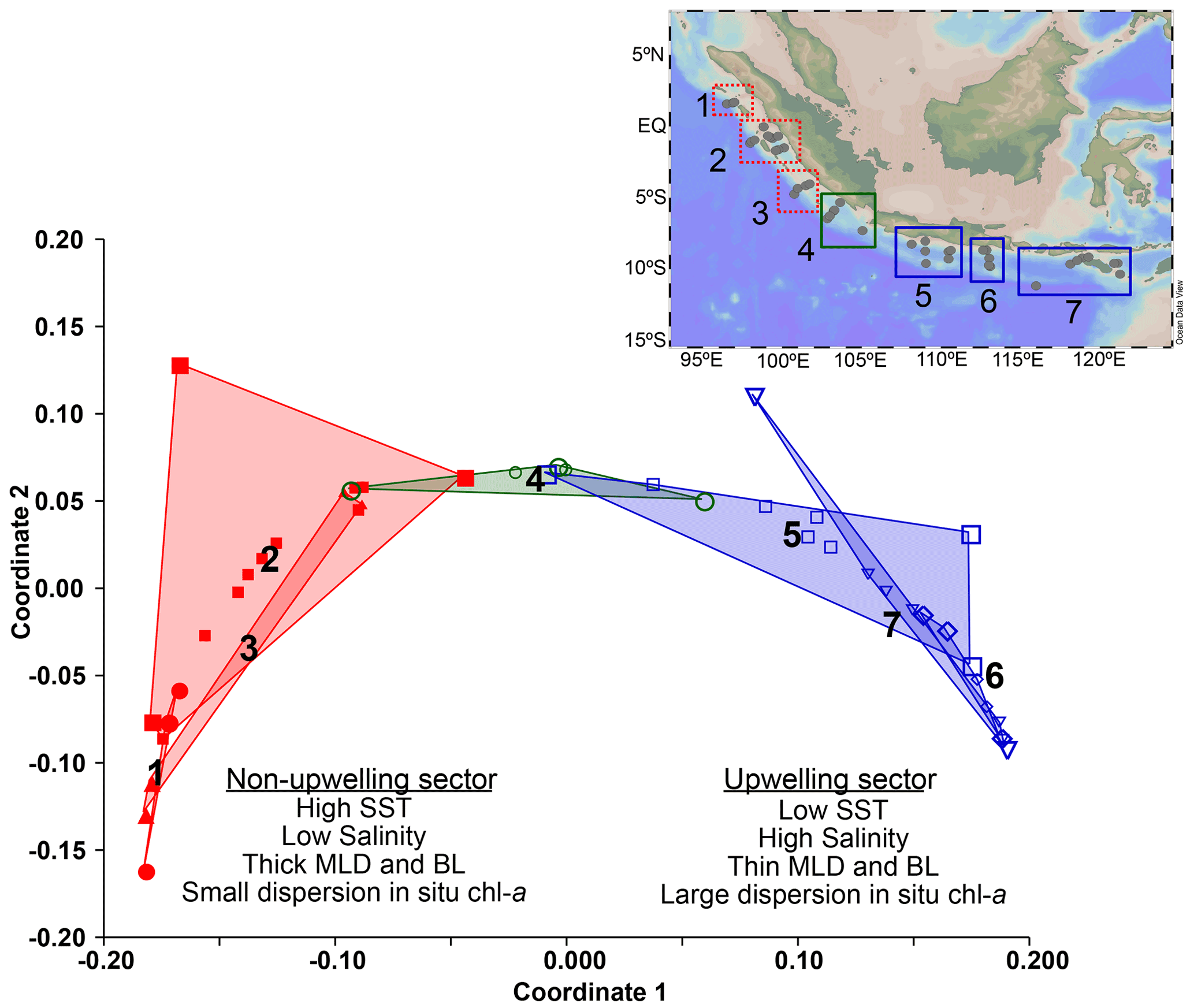
Figure 3Non-metric multidimensional scaling of the in situ hydrographic parameters shows three main clusters. Cluster 1 includes transects 5 to 7 off Java and the LSI influenced by upwelling (upwelling; blue). Cluster 3 includes transects 1 to 3 located off Sumatra which are not influenced by upwelling (non-upwelling; red). Cluster 2 consists of only transect 4, which represents a transitional condition between Sumatra and Java–LSI (green). Locations of the stations are shown in the inset at the top right corner of the figure.
Planktic foraminiferal assemblage and absolute abundance
The total composition of the planktic foraminiferal species comprises 29 morphospecies. Eleven morphospecies, namely Globigerina bulloides, Globigerinella calida, Globigerinita glutinata, Globigerinoides ruber (white), Trilobatus trilobus, Globorotalia menardii, Neogloboquadrina dutertrei, Globorotalia hirsuta, Globigerina falconensis, Pulleniatina obliquiloculata, and Globigerinella siphonifera, accounted for 90 % of the total assemblage (Fig. 4a). The abundance of planktic foraminifera ranges from ∼3 to ∼80 individuals m−3, and shows a strong zonal divide (Fig. 4b and c). The lowest abundances, with median values ranging between ∼4 and ∼12 individuals m−3, occur off Sumatra (transects 1–3) (Fig. 4b and c), while the highest abundances, with median values ranging between 18 and 35 individuals m−3, occur off southern Sumatra and Java–LSI (transects 5–7) (Fig. 4b and c).
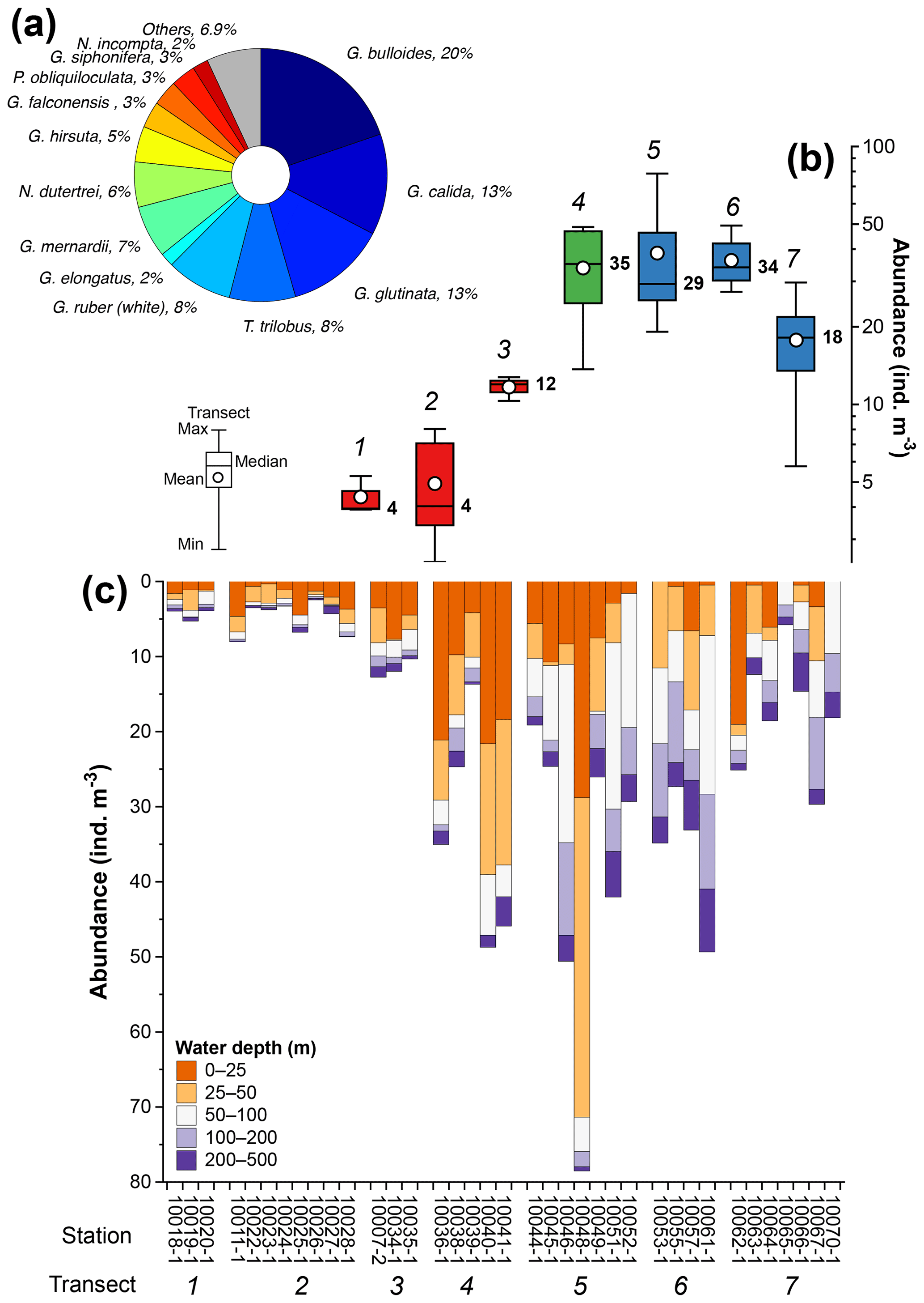
Figure 4Summary of planktic foraminifera census counts off Indonesia. (a) Species with >2 % contribution to the total assemblage, (b) abundance distribution of planktic foraminifera in transects 1 to 7, and (c) abundance of planktic foraminifera by water depth interval at each station. Numbers in (b) represent transects 1 to 7 (italic) and median values of transects (bold); colors in (b) depict sectors off Sumatra (red), transitional sectors (green), and off Java–LSI (blue). The five sampled water depths are 0–25 m (tangerine), 25–50 m (orange), 50–100 m (white), 100–200 m (lilac), and 200–500 m (purple). Stations are grouped by transect (number). Schematic of the box plots showing the median value (horizontal line); the whisker marks the minimum (min) and maximum (max) values. White dots denote the mean of data distribution. Note the difference between the mean and median, where the former is more susceptible to extreme low and high values. Please note the different scales for the y axis in (b) (log scale) and (c) (linear scale).
3.2 Vertical distribution of paleoceanographically relevant species
Similar to the spatial pattern of total abundance in each transect (Fig. 4b), the vertical dispersion of planktic foraminifera abundance across the water column shows a strong zonal pattern (Fig. 5a). Off Sumatra, the vertical distribution of planktic foraminiferal abundance is characterized by a high concentration in the upper 50 m (i.e., >30 % of the total abundance) and a rapid decrease toward deeper levels, with ≤15 % of the total abundance occurring between 50 and 500 m water depth. Meanwhile, off Java and the LSI, planktic foraminifera can be found throughout the upper 500 m of the water column. Unlike for stations off Sumatra, here the first 50 m of water column is relatively poor in planktic foraminifera, and the highest concentration (>20 % of the total abundance) occurs between 50 and 100 m water depth. This general pattern is true for all stations off Java–LSI except station GeoB10062-1 (Fig. 4c).
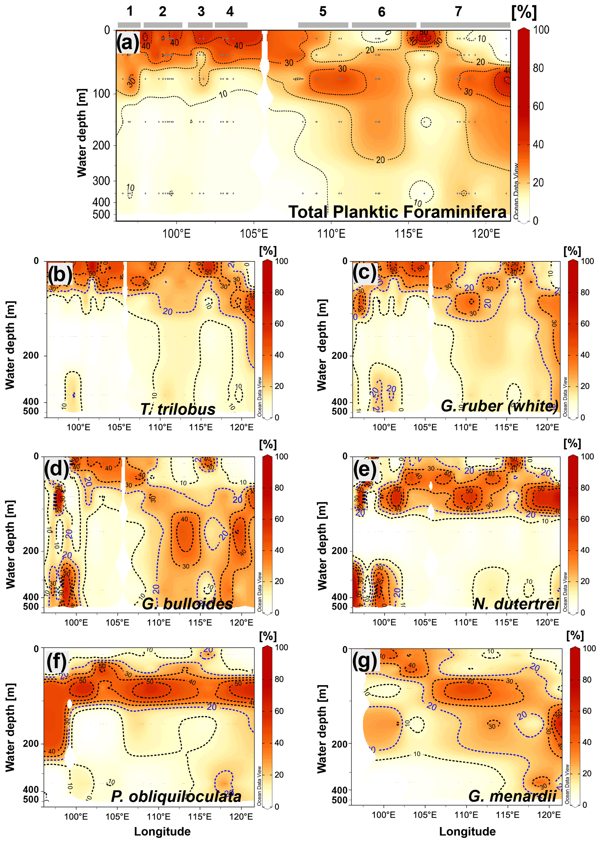
Figure 5Cross-sections showing the vertical distribution across the water column of (a) the total community of planktic foraminifera and the species, (b) T. trilobus, (c) G. ruber (white), (d) G. bulloides, (e) N. dutertrei, (f) P. obliquiloculata, and (g) G. menardii. Numbers and horizontal lines on top of (a) show each transect (1 to 7). Visualization is based on Ocean Data View 5.2.1 (Schlitzer, 2021).
In the following section, we describe the vertical distribution of six species of planktic foraminifera that are typically used in paleoceanographic studies (for example, Caley et al., 2012; Ding et al., 2013; Mohtadi et al., 2017; Steinke et al., 2014; Tapia et al., 2019), namely T. trilobus, G. ruber (white), G. bulloides, N. dutertrei, P. obliquiloculata, and G. menardii. Trilobatus trilobus exhibits a surface distribution with most of the organisms dwelling in the upper 50 m of the water column. Interestingly, some differences in their vertical distribution can be observed between sectors (i.e., Sumatra vs. Java–LSI) (Fig. 5b). In the Sumatra sector, T. trilobus is highly concentrated within the upper 30 m of the water column, showing a small vertical dispersion as its occurrence below 75 m is rare (Fig. 5b). Meanwhile, offshore Java and the LSI, T. trilobus shows a larger vertical dispersion with a relatively high concentration as deep as 100–200 m (Fig. 5b). The vertical distribution of G. ruber (white) shares some similarities with T. trilobus, that is, high concentration of specimens within the first 50 m of the water column off Sumatra and a larger dispersion off Java and the LSI (Fig. 5c). However, the vertical distribution of G. ruber (white) off Java suggests an even larger vertical dispersion than that of T. trilobus as G. ruber (white) shows that the isocline depicting 20 % of the population stretches from 100 to 400 m water depth (Fig. 5c). Globigerina bulloides shows no clear pattern in its vertical preference off Sumatra, occupying both upper and lower depths. In contrast, off Java and the LSI this species seems to prefer water depths below the thermocline between 100 and 350 m (Fig. 5d). Pulleniatina obliquiloculata and N. dutertrei (Fig. 5e and f) show a similar distribution, with a high occurrence of individuals between ∼50 and ∼100 m water depth. This feature seems to be constant throughout the study area. Although G. menardii is found mostly below 30 m water depth, its vertical distribution deepens along the study area, from dwelling at ∼50 m water depth off Sumatra to ∼150 m water depth off Java–LSI (Fig. 5g). Overall, abundance distribution of the selected species across the water column agrees with previous studies that categorize these species as surface-mixed-layer dwellers (T. trilobus and G. ruber (white)) or as deep-thermocline dwellers (N. dutertrei, P. obliquiloculata, and G. menardii) (Birch et al., 2013; Faul, 2000; Hemleben et al., 1989; Lessa et al., 2020; Rebotim et al., 2017; Steph et al., 2009).
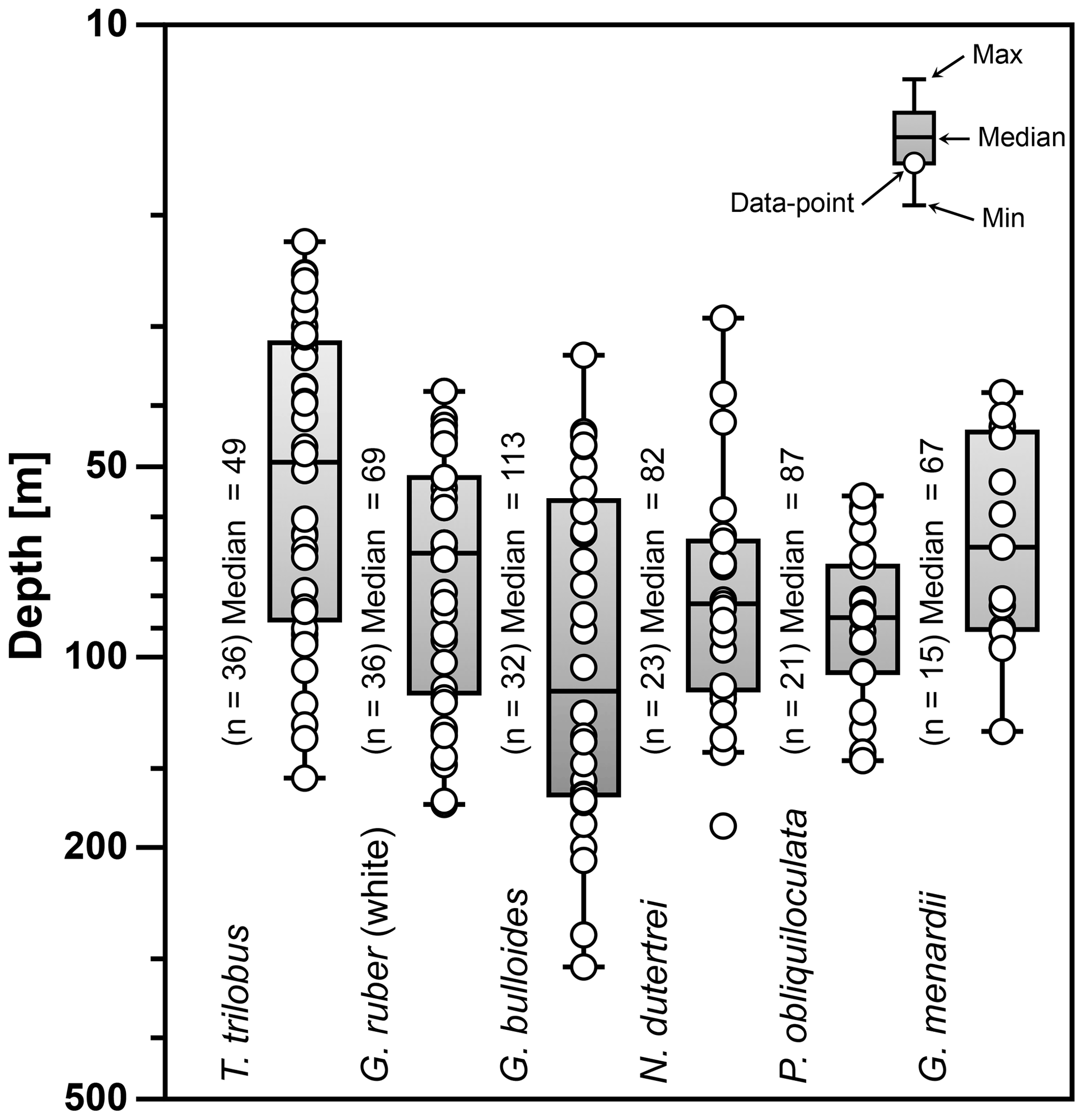
Figure 6Average living depth (ALD) of the species T. trilobus, G. ruber (white), G. bulloides, N. dutertrei, P. obliquiloculata, and G. menardii. The calculation includes only stations with more than five specimens per species (n). Schematic of the box plots showing the median value (horizontal line); the whisker marks the minimum (min) and maximum (max) values. Symbols (white circles) depict the ALD values. Note log scale for y axis.
The ALD calculated from the total abundance (living + dead specimens) of the selected species ranges between 47 and 113 m water depth (Fig. 6). The ALD for G. menardii, N. dutertrei, and P. obliquiloculata indicates that the habitat depth of these species is located between ∼67 and ∼87 m. The ALD value for G. bulloides suggests that the habitat depth of this species in the study area is ∼113 m, much deeper than the mixed layer in the study area. Meanwhile, the ALD for mixed-layer species is ∼49 m for T. trilobus and ∼69 m for G. ruber (white), respectively. Interestingly, the ALD of surface-dwelling G. ruber (white) is similar to that of some thermocline-dwelling species.
4.1 Planktic foraminiferal abundance and assemblage off Indonesia
The total number of species (n=29, size fraction >150 µm) observed in the plankton net samples collected during August and September 2005 is higher than the number of species observed in the surface sediments off Indonesia (n=18, size fraction >150 µm) (Ding et al., 2006) but lower than that observed in a sediment trap off Java (n=37, size fraction >150 µm) (Mohtadi et al., 2009). Higher diversity in our data compared to those of Ding et al. (2006) may be due to the loss of fragile and dissolution-prone species (e.g., Hastigerinella digitata, Turborotalita humilis, Globigerinita uvula) in the sedimentary record since only 4 of the 13 sites collected from the upwelling area off Java by Ding et al. (2006) are above the lysocline (∼2400–2800 m water depth) (Ding et al., 2006; Mohtadi et al., 2007). On the other hand, the longer temporal interval spanned by sediment trap samples off Java (3 months) compared to our sampling period (6 weeks) makes it possible to collect species with sporadic occurrence throughout the year. A recent global compilation study which includes the sediment trap data from Indonesia reported a warm bias in the assemblage due to anthropogenic effects and the likelihood that the water column may have changed over the last few decades (Jonkers et al., 2019). We note that their approach is based on the biogeography of planktic foraminifera; i.e., each species occupies a specific thermal niche, which may span a temperature range of >10 ∘C for some tropical species. On the other hand, our main findings about the habitat depth and implications for paleoclimate reconstruction are based on individual species. The selected species are not dwelling at the limit of their thermal niche; thus as long as these species do not substantially shift their thermal niche over time, we do not expect any large bias due to the reported anthropogenic changes in foraminiferal assemblage.
The abundance of planktic foraminifera in the upwelling sector of Java–LSI is 4 to 8 times higher than that in the non-upwelling Sumatra sector (Fig. 4b). Higher foraminiferal abundance in the presence of upwelling is consistent with previous studies and is likely due to higher food availability when upwelling occurs (Kimoto, 2015; Schiebel and Hemleben, 2005; Schiebel et al., 2001). Species such as G. bulloides, G. glutinata, and G. falconensis have been classified as species associated with upwelling conditions, and their abundances are positively correlated with the intensity of the upwelling (Brock et al., 1992; Cayre et al., 1999; Conan and Brummer, 2000; Sautter and Sancetta, 1992). Species such as N. dutertrei, P. obliquiloculata, and G. menardii normally live in nutrient-rich waters below the mixed layer in the thermocline (Sautter and Thunell, 1991). Meanwhile, T. trilobus and G. ruber (white) occur in areas with a thick mixed layer. These mixed-layer dwellers have many similarities, including life span (of 2 to 4 weeks), feeding strategies, and reproduction synchronized with the synodic lunar cycle (Schiebel and Hemleben, 2017, and references therein). Compared to T. trilobus, which predominantly occurs under warm oligotrophic conditions, G. ruber (white) displays a more opportunistic behavior as this species can be abundant and occurs in a larger range of trophic conditions, from oligotrophic to eutrophic due to its ability to feed on a greater variety of food sources (Schiebel and Hemleben, 2017; Schiebel et al., 2018).
Off Sumatra without upwelling, G. ruber (white), G. elongatus, and T. trilobus account for ∼44 % of the total assemblage, while the species associated with high productivity or upwelling conditions have a minor presence (G. bulloides (∼8 %) and G. glutinata (∼9 %)) or are rare to absent (N. dutertrei, <2 %) (Fig. 7a). On the other hand, off Java and the LSI, where upwelling occurs, the assemblage composition is strongly dominated by G. bulloides (21 %); G. glutinata (14 %); and the deep-dwelling species associated with high productivity, i.e., N. dutertrei, G. menardii, and P. obliquiloculata, together contributing 18 % of the total assemblage. Trilobatus trilobus and G. ruber (white), contribute only 7 % and 8 %, respectively, of the total assemblage off Java and the LSI (Fig. 7b).
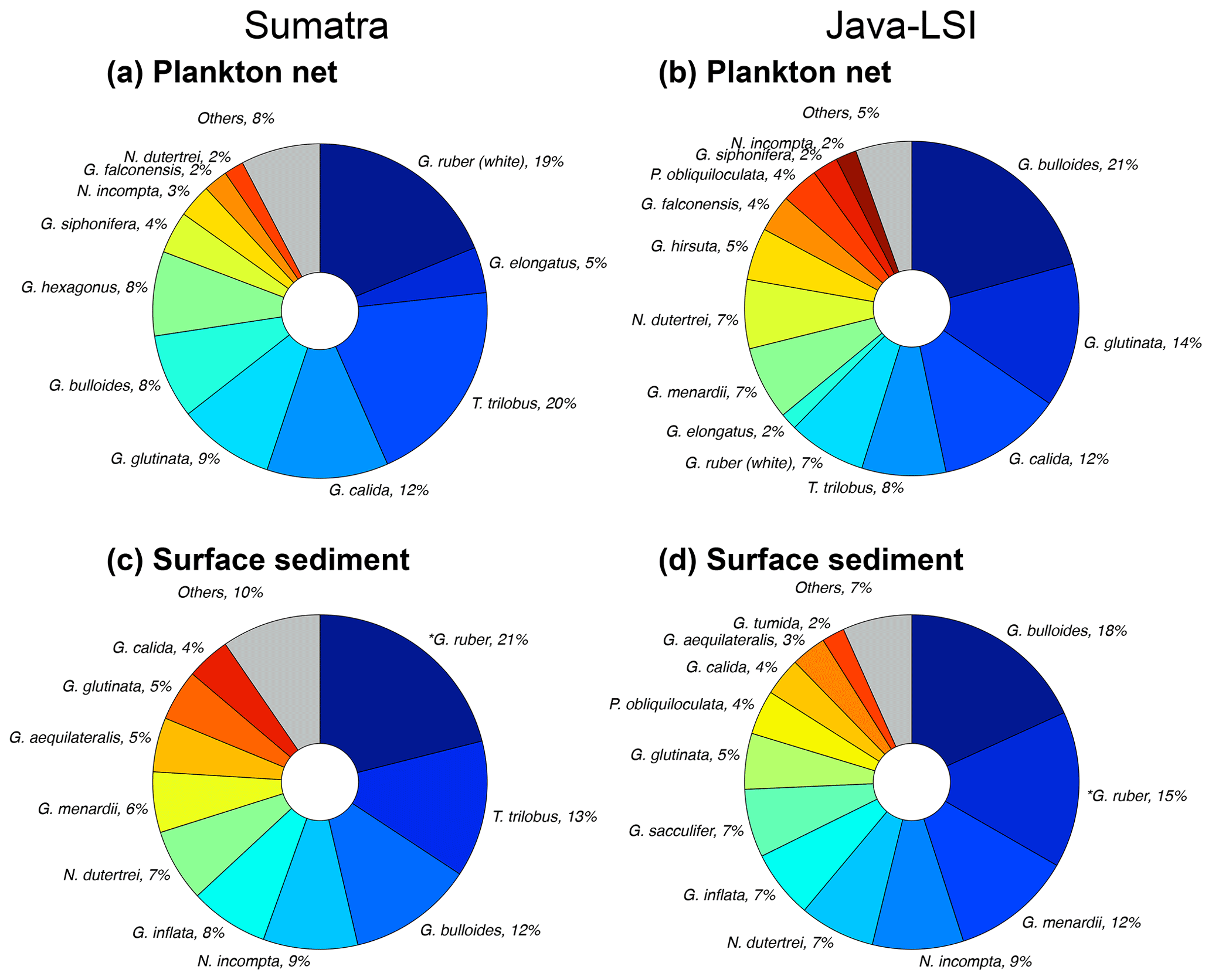
Figure 7Planktic foraminiferal assemblage in samples of (a, b) plankton nets (this study) and (c, d) surface sediments (data from Mohtadi et al., 2007) off Sumatra (transect 1–3) and off Java–LSI (transect 5–7). Mohtadi et al. (2007) did not differentiate between morphotypes; *G. ruber data comprise both morphotypes (G. ruber (white) + G. elongatus). Note that G. ruber (white) and G. elongatus data from plankton nets are plotted side by side to facilitate visual comparison with *G. ruber in sediment data.
Interestingly, despite methodological differences (sampling season and water depth, size fraction analyzed), our results are broadly consistent with those of a plankton net study carried out here in late autumn–early winter of 1963 at the end of the upwelling season (Ujiié, 1968). Ujiié found that the assemblage of planktic foraminifera off Java consisted of a mixture of species associated with nutrient-rich and nutrient-poor waters, dominated by N. dutertrei (28 %), G. ruber (22 %), and T. trilobus (10 %). On the other hand, off Sumatra (100∘ E) oligotrophic species T. trilobus and G. ruber accounted for 56 % of the total assemblage of planktic foraminifera. Thus, the assemblage and dominant species characterizing these two sectors seem to persist until the end of the upwelling season. The spatial contrast in the composition and abundance of planktic foraminiferal species (Figs. 4 and 7) in upwelling vs. non-upwelling conditions suggests that the hydrographic changes related to upwelling govern the distribution of planktic foraminifera. This finding is consistent with previous studies suggesting that off Indonesia, seasonal upwelling plays a critical role in modulating the ecology of planktic foraminifera (Ding et al., 2006; Mohtadi et al., 2007, 2009, 2011; Ujiié, 1968). Consequently, foraminiferal abundances (Fig. 4b) and species composition in plankton net samples collected during the SE monsoon season reflect the transition, in space, from oligotrophic, deep-mixed-layer and more stratified upper-water-column conditions (Sumatra) to a more eutrophic, shallow mixed layer and well-mixed upper water column (Java and the LSI). The transition zone between the two hydrographic regimes for the period August–September is located off the Sunda Strait (∼103 – ∼105∘ W) (Fig. 1c) (Susanto et al., 2001). Altogether, the aforementioned observations suggest that changes in the temporal extent, intensity, and zonal coverage of the seasonal upwelling might have a profound effect on the ecology of planktic foraminifera in the study area. Interestingly, the zonal divide in planktic foraminiferal assemblage between non-upwelling and upwelling regions observed in our net data is also reflected to some degree in surface sediments (Fig. 7c and d). Similar to what we observed in the plankton net data of the SE monsoon, the assemblage in sediments off Sumatra is dominated by G. ruber (white), while that off Java is dominated by G. bulloides. However, the proportion of less dominant species differs for plankton net and sediment samples. For instance, G. calida constitutes 12 % of Java net samples but only 4 % in the sediments. This discrepancy may reflect a different temporal coverage of these two sample types; i.e., surface sediments integrate over tens to hundreds of years, whereas net samples provide only a “snapshot” of the sampling period during the SE monsoon. The test of G. calida is relatively fragile; thus post-depositional processes like carbonate dissolution may also bias the assemblage in sediments (Ding et al., 2006). The effect of dissolution is likely not severe as most of the stations are above the lysocline (Mohtadi et al., 2007), and some G. calida are found in sediments (Ding et al., 2006), albeit at a lower proportion than in our plankton net data.
4.2 Planktic foraminifera habitat depth off Indonesia
Processes such as daily vertical migration and reproduction may play a role in the vertical distribution of planktic foraminifera. The effect of daily vertical migration cannot be properly assessed by our sampling design, but there is strong evidence that argues against daily vertical migration in planktic foraminifera (Meilland et al., 2019). However, it cannot be excluded that lateral patchiness of foraminiferal occurrence affects the vertical distribution, as proposed recently by Meilland et al. (2019). To buffer against this potential caveat as well as potential bias due to dead specimens collected at depths (details in Sect. 2.2), we interpret data averaged over several stations within each individual transects.
In the case of a modified vertical distribution due to synchronized reproduction – if some species reproduced consistently in phase with the full moon (Schiebel and Hemleben, 2017) – changes in the size class distribution should be noticeable before and after the occurrence of a full moon during the sampling period. Among all the species selected, G. ruber (white), N. dutertrei, and G. menardii show changes in their size class distribution consistent with this pattern (Fig. A2). The other species show equal distribution of the larger and smaller size fractions before and after a full moon. We note that samples off Sumatra (Java–LSI) were collected before (after) the full moon, making it difficult to disentangle the effect of hydrography and synchronized reproduction. Although we cannot completely rule out ontogenic vertical migration, the lack of coherence between the calculated ALDs and the moon phase argues against ontogenic vertical migration as a primary driver of the habitat depth distribution in the study area.
The discussion in the following sub-sections focuses on species that are commonly used in geochemical analyses for paleoceanographic reconstruction, namely G. ruber (white), T. trilobus, N. dutertrei, P. obliquiloculata, G. menardii, and G. bulloides. Importantly, the habitat depth of these species was also the focus of several previous studies in the region based on a sediment trap and surface sediments (Mohtadi et al., 2007, 2009, 2011).
4.3 Dominant species in nutrient-poor waters: G. ruber and T. trilobus
Many studies have shown that G. ruber (white) and T. trilobus have mixed-layer habitat preferences in oligotrophic conditions (Bé, 1977; Duplessy et al., 1981; Fairbanks et al., 1980; Kuroyanagi and Kawahata, 2004); thus they are considered reliable recorders of changes in the surface ocean at different timescales. However, the habitat depth of these species may change from area to area depending on the local hydrography, e.g., the depth of the mixed layer (Schiebel and Hemleben, 2017, and references therein).
The calculated habitat depth for G. ruber (white) (median=69 m) (Fig. 6) is deeper than the habitat depth estimated from surface sediments for the study area (20–50 m) (Mohtadi et al., 2007, 2011). In contrast, the calculated habitat depth for T. trilobus (median=49 m) (Fig. 7) is similar to the calcification depth estimated using surface sediments off Indonesia (∼50 m) (Mohtadi et al., 2011). The relatively great habitat depth shown by G. ruber (white) may be related to the lack of living planktic foraminifera specimens and the use of total counts in the calculation of the ALD (see Sect. 2.2).
Previous studies have suggested that a deepening of the habitat depth due to the use of total counts can be considered marginal (Greco et al., 2019). For example, in the area influenced by the upwelling, including both live and dead (total) specimens in the calculation of ALD leads to an increase of only ∼4 to 15 m for G. ruber (Lessa et al., 2020; Rebotim et al., 2017). Similar overestimation, 2–13 m, in the habitat depth of T. trilobus is observed when dead specimens are included in the ALD, suggesting that the bias in ALD calculation caused by inclusion of dead specimens should be comparable across mixed-layer dwellers. Therefore, the inclusion of dead specimens may not necessarily result in a severe bias in the habitat depth estimates. Furthermore, the agreement in the habitat depth of T. trilobus inferred from sediments and our ALD calculation also suggests that dead specimens likely do not make up a large portion of the net samples; the same is probably true for G. ruber (white) from the same samples. Together, these observations suggest that the relatively deep ALD calculated for G. ruber (white) is likely a robust finding and not severely biased by the inclusion of dead specimens in the calculation.
4.4 Dominant species in nutrient-rich waters: N. dutertrei, P. obliquiloculata, G. menardii, and G. bulloides
Species such as N. dutertrei, P. obliquiloculata, G. menardii, and G. bulloides are normally associated with high food availability and dwell in the upper water column across the mixed layer and upper part of the thermocline (Schiebel and Hemleben, 2017, and references therein). The habitat depth based on ALD calculation of the deep-dwelling species, N. dutertrei (median=82 m) and P. obliquiloculata (median=87 m) (Fig. 7), shows a good agreement with the habitat depth inferred from both sediment trap time series and surface sediments, i.e., 75–100 m for N. dutertrei and 60–90 m for P. obliquiloculata, respectively (Mohtadi et al., 2009, 2011). These habitat depth estimates are close to the lower end of the range for these species in regions influenced by the Benguela and Canary upwelling system in the Atlantic Ocean, that is, ALDs of 52 ± 32 m for N. dutertrei and 45 ± 31 m for P. obliquiloculata, respectively (Lessa et al., 2020; Rebotim et al., 2017). Similarly, the habitat depth of G. menardii off Indonesia is also at the lower end of its habitat depth observed off Africa in waters influenced by the Benguela Upwelling System (ALD of 39 ± 22 m) (Lessa et al., 2020). Notably, of all the species only G. menardii shows a shallower habitat depth (median=67 m) (Fig. 8) than that inferred from sediment trap data (90 to 110 m) (Mohtadi et al., 2009). A habitat depth of 67–87 m water depth, for G. menardii, N. dutertrei, and P. obliquiloculata, places them just below the lower boundary of the mixed layer, which is on average 52 m (Table A1).
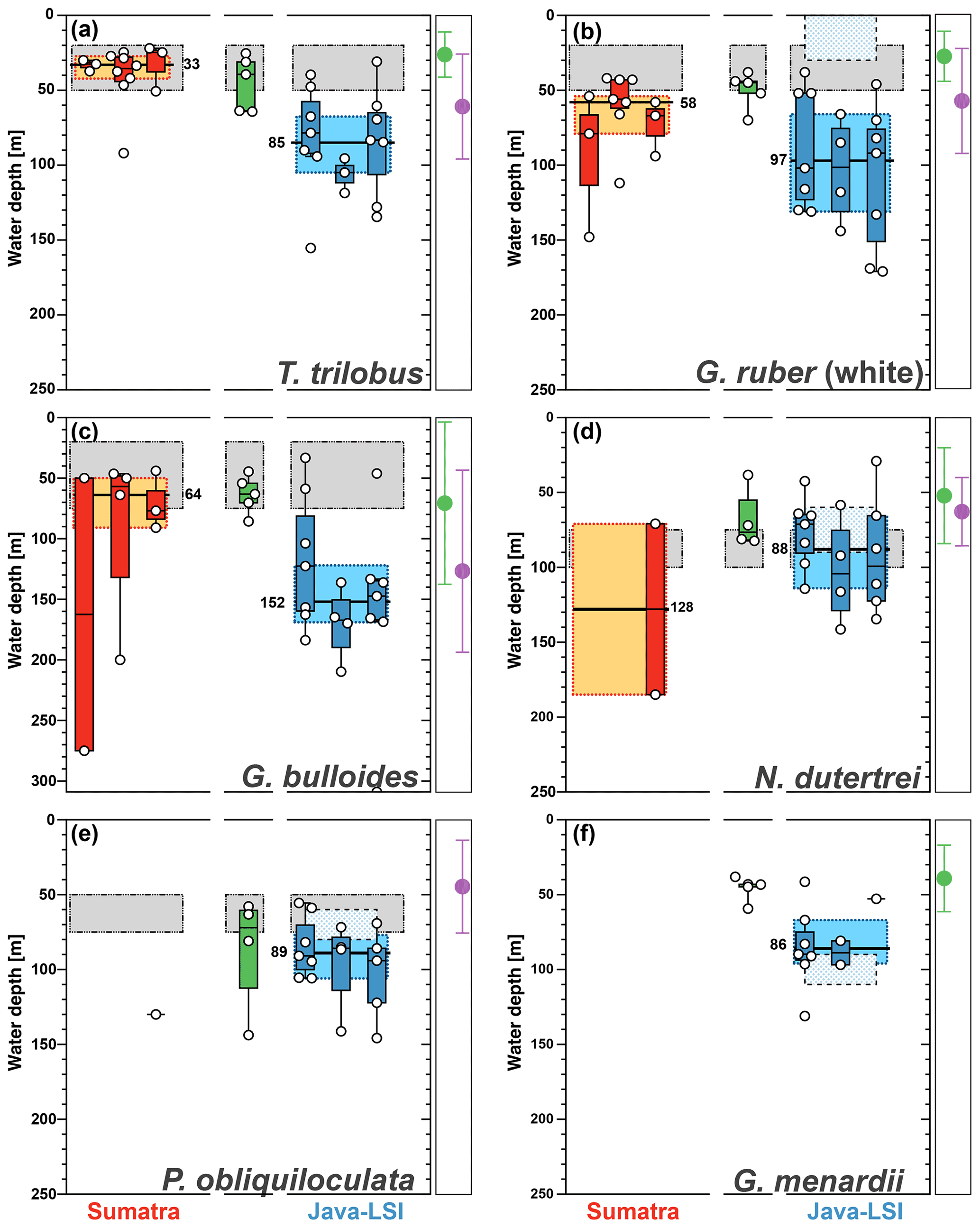
Figure 8Average living depth (ALD) distribution for (a) T. trilobus, (b) G. ruber (white), (c) G. bulloides, (d) N. dutertrei, (e) P. obliquiloculata, and (f) G. menardii per transect off Sumatra (red), in the transitional zone off southern Sumatra (green), and off Java–LSI (blue). The calculation only considers stations with more than five counts per species. The yellow and light-blue boxes depict the first and third quartiles of the ALD values off Sumatra (non-upwelling) and off Java–LSI (upwelling); black bars and numbers depict the median value per sector. Boxes depict the inferred vertical distribution from surface sediments (gray) along Indonesia and from the sediment trap (pattern) off Java (Mohtadi et al., 2009, 2011). Colored dots and vertical lines depict calculated mean ALDs and vertical dispersion based on living foraminifera data from areas influenced by the Benguela (green) and Canary (purple) upwelling systems (Lessa et al., 2020; Rebotim et al., 2017). ALDs for other species are presented in Fig. A3.
Globigerina bulloides has a median habitat depth of 113 m (Fig. 6); this value is almost twice the mean habitat depth estimated from surface sediments off Indonesia (∼50 m) (Mohtadi et al., 2011) and close to the low end of the observed habitat depth, i.e., 57 ± 10 to 102 ± 67 m, for this species in the Atlantic (areas under influence of Benguela and Canary upwelling) (Lessa et al., 2020; Rebotim et al., 2017). Globigerina bulloides is an opportunistic species whose abundance and habitat depth have been linked to food availability in the water column (Peeters and Brummer, 2002). Therefore, it is possible that its habitat depth follows the depths where food availability is the highest in the water column. The comparison of its median ALD value off Sumatra (non-upwelling) and off Java–LSI (upwelling) shows a deepening from ∼64 to ∼152 m, respectively. This finding suggests that regional differences in the habitat depth of some planktic foraminifera might occur as a result of seasonal upwelling.
4.5 Zonal differences in the habitat depth: non-upwelling vs. upwelling
Previous studies off Indonesia matching geochemical data (δ18Ocalcite) from core tops and water profiles have suggested differences in the habitat depth of some planktic foraminifera species between the sectors of Sumatra, Java, and the LSI (Mohtadi et al., 2007). Mohtadi et al. (2007) reported that off Sumatra, the G. ruber δ18O values reflected a habitat depth <50 m water depth, while off Java and the LSI the G. ruber δ18O values were “out of range” (<0 m water depth). The authors speculated that the out-of-range geochemical signature off Java most likely reflects a greater contribution during the non-upwelling period when the water is warmer, fresher, and more stratified. A similar situation was observed for N. dutertrei as its geochemical signature suggests a deeper habitat depth in the non-upwelling Sumatra sector (50–75 m) relative to the upwelling Java sector (20–50 m) (Mohtadi et al., 2007). The notion that the seasonal upwelling off Indonesia may trigger changes in the habitat depth of planktic foraminifera species is further supported by sediment trap data, wherein and δ18O data from planktic foraminifera (i.e., G. ruber, N. dutertrei, G. menardii, and P. obliquiloculata) vary with seasonal upwelling (Mohtadi et al., 2009). Therefore, the coherent, strong zonal shifts in the vertical dispersion of the selected planktic foraminifera in our plankton net samples (Fig. 5a–g) and hydrographic parameters (i.e., SST, MLD, salinity, and chl a) (Fig. 2a–c) in response to upwelling call for further scrutiny of potential zonal differences in the habitat depth values (Fig. 6).
The zonal disaggregation of the habitat depth (Fig. 8) into non-upwelling (transect 1 to 3) and upwelling (transect 5 to 7) sectors (see Sect. 3.1) shows that G. ruber (white), T. trilobus, and G. bulloides have a greater habitat depth in the upwelling sector than the non-upwelling sector. There is a 2-fold increase in their mean habitat depth (Fig. 8a–c) from the non-upwelling to upwelling sector, i.e., from ∼33 to ∼85 m for T. trilobus, ∼58 to ∼97 m for G. ruber (white), and ∼64 to ∼152 m for G. bulloides. This finding, i.e., differing habitat depths in upwelling vs. non-upwelling regions for T. trilobus and G. ruber (white), is further corroborated by the estimates of bootstrap 95 % confidence intervals and randomization tests with replacements (Table 1; details of calculation in the “Materials and methods” section). Compared to other species, the statistical significance of the ALD difference in G. bulloides is less strong (P=0.057), likely due to the large spread in the vertical dispersion of this species. Although deeper than usually assumed for paleoceanographic reconstructions, the ALD values for G. ruber (white), T. trilobus, and G. bulloides in the upwelling sector are indeed within the ranges previously reported elsewhere for areas influenced by upwelling (Lessa et al., 2020; Rebotim et al., 2017) (see Sect. 4.2). A clear zonal divide can be observed, i.e., shallow ALD values occurring off Sumatra (non-upwelling) vs. deep ALD values occurring off Java–LSI (upwelling). Transect 7 in the LSI is in addition to monsoonal upwelling also under the influence of the ITF as it allows the passage of cooler and fresher water (Tillinger, 2011). The habitat depth of mixed-layer dwellers here is not the deepest in the upwelling region, despite the low presence of mixed-layer dwellers (G. ruber (white) and T. trilobus) in the upper 50 m during the sampling period (Fig. 5), especially at stations GeoB10065 and GeoB10070 (Fig. 4c). The ALD estimates of G. ruber (white) and T. trilobus at these two stations are the deepest along transect 7 (the two lowest data points in the panel for G. ruber and T. trilobus in Fig. 8). Station GeoB10070 is the easternmost site of the study, and thus it might be under a stronger influence of the ITF than the other stations along the transect. This is, however, not the case for station GeoB10065, which is flanked by several stations at which mixed-layer dwellers are present in the upper 50 m. Therefore, it is possible that the vertical distribution at these two stations is not representative of the transect nor of the influence of the ITF. Multivariate analysis also indicates that the hydrography at transect 7 is similar to that at transect 5 and 6, suggesting a negligible influence of ITF here. Although the calculated habitat depths of the surface dwellers off Sumatra (Fig. 8) show a relatively good fit with the estimated habitat depths based on geochemical data (δ18Ocalcite and temperatures) (Mohtadi et al., 2009, 2011), this is not the case for transects off Java and the LSI, where the overall lack of agreement between the sedimentary data and plankton net results is evident (Fig. 8a–c).
The low abundance of G. menardii, N. dutertrei, and P. obliquiloculata off Sumatra precludes ALD calculation and hence also the zonal comparison of their habitat depths (Fig. 8d–f) between Sumatra and Java–LSI. Despite their low abundance in net samples collected in August–September, these three species are found in relatively high abundances in surface sediments off Sumatra, constituting up to 13 % of the assemblage (Fig. 7c; Mohtadi et al., 2007). Thus, their occurrence offshore Sumatra might be temporally restricted to only the final part of the SE monsoon (October) when the upwelling center locked off the Sunda Strait starts drifting westward (Susanto et al., 2001), triggering higher productivity offshore Sumatra. Alternatively, they might represent the positive IOD or El Niño years, when upwelling is generally stronger in the eastern Indian Ocean and reaches further northerly latitudes. Off Java, where their abundance is sufficiently high for ALD calculation, the data suggest that these three species share a similar niche at thermocline depths centered at ∼90 m water depth, in agreement with the habitat depth inferred from surface sediments (Fig. 8d–f).
4.6 Implications for paleoceanographic reconstructions
Field observations (plankton net and sediment trap data) provide insights into the modern ecology of planktic foraminifera as the habitat depth of some species is known to vary in time and at regional scale (Schiebel and Hemleben, 2017). Our plankton net data show that the habitat depth of mixed-layer-dwelling G. ruber (white) and T. trilobus deepens in upwelling conditions, while thermocline-dwelling N. dutertrei and P. obliquiloculata thrive only in the upwelling region off Java and the LSI.
As with many zooplankton, the abundance of planktic foraminifera is linked to food availability; thus some species may change their habitat depth to maximize food acquisition. The habitat depth of symbiont-bearing species like T. trilobus and G. ruber is typically assumed to be restricted to the surface ocean or at least within the photic zone as they rely on their photosynthetic symbionts for nutrition. In addition, these species also catch prey and feed on a wide variety of food sources (Hemleben et al., 1989, and references therein), plausibly because the photosynthates produced by the symbionts are insufficient to sustain the growth of the host (Bé et al., 1981; Caron et al., 1982). Indeed, a recent study showed that the nutritional contribution of the symbionts to the host is significantly smaller than that obtained by ingesting copepods, implying that the photosymbiosis in planktic foraminifera may not be the primary source of energy when prey is abundant (Takagi et al., 2018).
During the SE monsoon, the photic zone ranges between ∼50 and ∼75 m, and the food availability off Java and the LSI is high due to the enhanced predator–prey encounter fueled by the high phytoplanktonic biomass across the water column and upwelling-induced vertical mixing (Pécseli et al., 2014). Under this circumstance, it is plausible that omnivorous mixed-layer dwellers like T. trilobus and G. ruber (white) might adopt a feeding strategy that includes both photosymbiosis and preying, or even primarily the latter. Preying on other zooplanktons like copepods, which have ontogenic and daily migration through the water column, means that planktic foraminifera are not limited to the photic zone for food. Moreover, copepods have been found to shift to a deeper habitat as a strategy to maximize their retention within a coastal upwelling area (Peterson, 1998; Peterson et al., 1979; Verheye et al., 1991). In combination, the aforementioned factors may thus lead to a greater habitat depth for mixed-layer dwellers in the upwelling region off Java compared to the non-upwelling region off Sumatra.
The thermal gradient between mixed-layer- and deep-dwelling species (ΔT) is commonly used as a proxy for the thickness of the mixed layer and the position of the thermocline in the water column on glacial–interglacial timescales (Farmer et al., 2011; Mohtadi et al., 2017; Steinke et al., 2014; Tapia et al., 2015). The ΔT calculated from the abundance-weighted temperatures of our plankton net data shows that during the SE monsoon larger ΔT values occur off Sumatra than off Java–LSI where upwelling occurs (Figs. 9 and 10). Due to its relatively great habitat depth off Java–LSI, the abundance-weighted temperature derived from surface-dwelling G. ruber (white) and T. trilobus is comparable to that of thermocline-dwelling species and substantially lower than that of their counterpart off Sumatra. The habitat depth change in the mixed-layer species is thus the primary reason for the ΔT difference between the two sectors. Interestingly, smaller ΔT during upwelling conditions is also evident in the flux-weighted data from a sediment trap off Java (Figs. 9 and 10), which show that the ΔT reduces from 4.3 ∘C during the non-monsoon period to 1.2 ∘C during the seasonal upwelling period (SE monsoon) (Mohtadi et al., 2011). Although both plankton net and sediment trap data are based on suspended or sinking foraminifera in the water column, they reflect a different signal in time and space; our net data reflect a spatial difference during the sampling period spanning 6 weeks during the monsoonal upwelling season, while the trap data reflect temporal changes at one location that is under the influence of monsoonal upwelling. Despite their inherent differences, both datasets, however, show that off Indonesia ΔT decreases as a function of upwelling dynamics. A more well-mixed upper water column in upwelling conditions, hence smaller surface–subsurface temperature difference, is also reasonable taking into account the weaker water column stratification during upwelling (Fig. 10). The latter is due to a thinner barrier layer and a shallower MLDTEMP (Fig. 2a and Table A1). This finding indicates that ΔT may be a useful proxy for reconstructing past upwelling conditions off Indonesia if the foraminifera produced during the upwelling season dominate foraminiferal test abundance in the sediments.
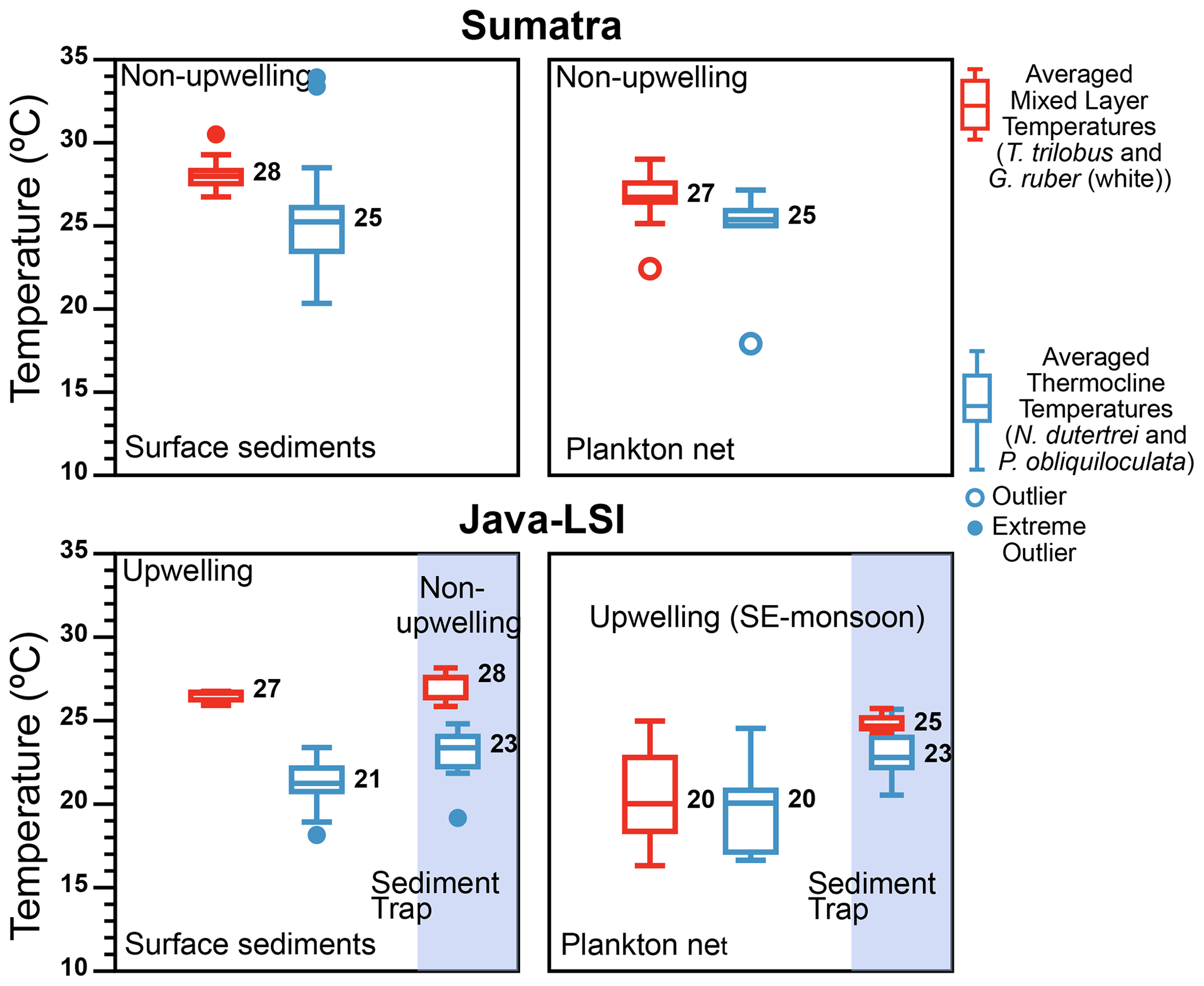
Figure 9Comparison of the thermal gradient (ΔT) off Indonesia inferred from surface sediments ( data from Mohtadi et al., 2011), plankton net (abundance-weighted temperatures; this study), and sediment trap ( data from Mohtadi et al., 2009). During the SE monsoon the ΔT calculated from the plankton net data shows that larger ΔT values occur off Sumatra (non-upwelling) than off Java (upwelling), in agreement with the seasonal ΔT off Java calculated from sediment trap (circles) with larger ΔT occurring during the non-upwelling season than the upwelling season. The color represents the inferred averaged temperatures for the mixed layer (combining G. ruber and T. trilobus; red) and thermocline (combining N. dutertrei and P. obliquiloculata; blue); numbers represent median values. Outliers and extreme outliers, >1.5 and >3 times the interquartile range, are depicted by filled and open circles, respectively.
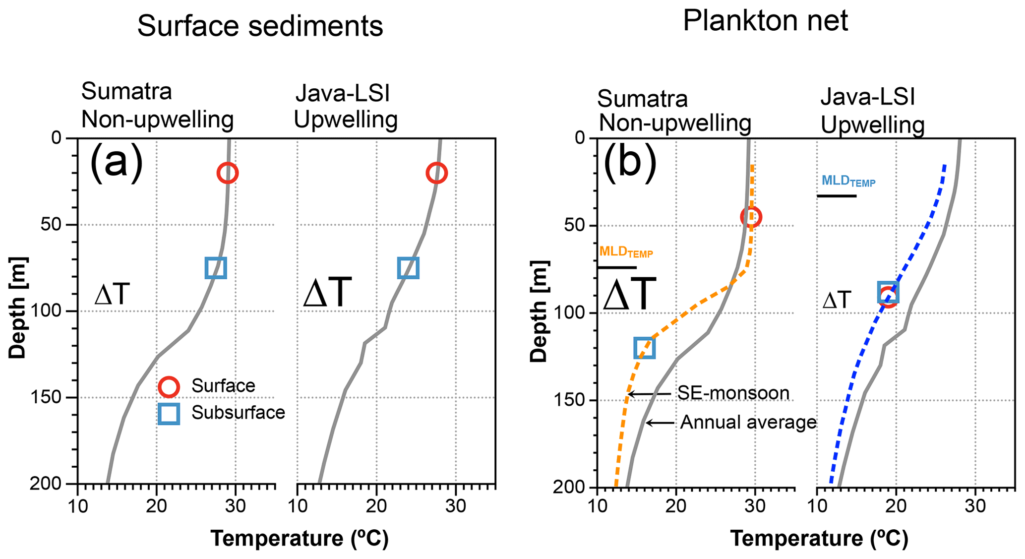
Figure 10Schematic comparing the ΔT derived from mixed-layer and thermocline dwellers off Sumatra and Java–LSI, from (a) surface sediment (inferred habitat depth from Mohtadi et al., 2011) matching the mean annual conditions and (b) ALD from plankton net matching the water column structure during the sampling period (SE monsoon, August–September 2005). Gray lines depict the average annual mean water column structure offshore Sumatra and Java–LSI (band of 160 km wide, >200 stations from WOA2018, 0.25∘) (Locarnini et al., 2018); dashed lines depict the average water column structure in each sector during the SE monsoon based on in situ data collected during the PABESIA cruise (August–September 2005); the black line shows the average depth of the MLDTEMP (Table A1).
Mohtadi et al. (2009) showed that ∼50% of the total annual foraminiferal flux off Java occurs during the SE monsoon season, and the fluxes during this season are largely centered around September, suggesting that our “snapshot” may be reasonably representative of the foraminiferal response to the prevailing ocean conditions during the SE monsoon off Indonesia. Geochemical data (δ18Ocalcite and inferred temperatures) in marine sediments off Java show a broad agreement with the habitat depth estimates from our plankton net data for subsurface dwellers (Fig. 8), but not for mixed-layer-dwelling species. Plankton net data suggest a greater habitat depth for the mixed-layer species and hence also lower inferred temperature. As a result, the ΔT off Java–LSI calculated from the plankton net data is smaller than that of surface sediment data. The situation differs off Sumatra, where the habitat depth estimates for both mixed-layer and subsurface species derived from marine sediments and plankton net samples are in agreement and hence also the derived ΔT. Consequently, the zonal reconstruction of the ΔT based on surface sediments indicates a larger ΔT off Java–LSI than off Sumatra (Mohtadi et al., 2011), in contrast to that of our net data (Figs. 9 and 10). In other words, surface sediment data suggest larger ΔT values in regions influenced by strong seasonal upwelling.
This discrepancy between surface sediment and plankton net data off Java may stem from the different temporal intervals integrated by each sample type and the fact that calcification depth inferred from the surface sediment may not be synonymous with the habitat depth inferred from plankton net data. The plankton net data reflect the conditions in the water column sampled during the SE monsoon and thus can be directly linked to the hydrographic processes that occurred during sampling. To some extent this is also true for sediment trap samples; a limited temporal interval integrated by the samples at one location means that process attribution can be better constrained. On the other hand, marine sediments integrate foraminiferal flux over tens to hundreds of years, depending on the local sedimentation rate, and may be susceptible to post-depositional processes such as dissolution, bioturbation, and reworking, which may alter the proxy signal. Together, these issues make it challenging to quantify the relative importance of each process and thus to ground-truth proxies. Nonetheless, paleoceanographic reconstructions are based on sedimentary material, which may have undergone the same post-depositional processes as the surface sediments. If the relative importance of these processes would stay unchanged over time, then surface sediments are arguably the best modern analogue for paleoceanographic reconstruction. In this case, stronger upwelling off Indonesia is characterized by a larger (ΔT) as indicated by the zonal pattern of surface sediments (Figs. 9 and 10). However, were the fluxes of planktic foraminifera and the post-depositional processes to change over time, it is within the realm of possibility that under some circumstances, e.g., strong positive IOD or El Niño years, the proxy signal produced in the water column during one-off events like upwelling can be preserved in the sediments, especially if the resultant flux increases exponentially. Our findings highlight the need to consider multiple sample types to further constrain the analog used for downcore paleoceanographic reconstructions. To further shed light on the transfer of the proxy signal from the water column to the sediment, longer sediment trap time series and repeated plankton net sampling in the same region would be useful to capture the seasonality of the vertical distribution of planktic foraminifera. Importantly, generating geochemical data on plankton net samples may help to verify the habitat depths and allow a direct comparison with the depth inference from the surface sediments. It would also be helpful to constrain the age of surface sediments to ensure that they are comparable to modern data.
We examined the zonal and vertical distribution of planktic foraminifera off Indonesia during the boreal summer of 2005 at 37 stations. The stations were grouped into seven land–sea transects off Sumatra and off Java–LSI. The factors driving the observed distribution of foraminifer species were assessed using vertically resolved environmental data.
Twenty-nine species were identified that can be divided into two basic communities, i.e., one dominated by warm-oligotrophic-stratified-water-column species vs. cooler-eutrophic-well-mixed-water-column species. Similarly, foraminiferal abundance shows contrasting distributions off Sumatra and off Java–LSI. The concurrent zonal shift in abundance and species composition of planktic foraminiferal and environmental parameters (SST, chl a, MLD, and BL) in response to upwelling implies a close link between upwelling and the ecology of planktic foraminifera in this area. Similar to the abundances and species composition of planktic foraminifera, their vertical distribution across the water column shows a strong zonal differentiation, i.e., shallow depths–low dispersion off Sumatra vs. deeper depths–larger dispersion off Java–LSI.
The calculated ALDs of the selected species are in broad agreement with typically assumed habitat depths in paleoceanographic reconstructions, with the exception of G. ruber (white) and G. bulloides. The possibility of an overestimation due to possible inclusion of dead specimens in the calculation cannot be entirely ruled out at this point, but several lines of evidence suggest that a severe overestimation is not likely. The species G. ruber (white) and T. trilobus show a strong deepening in their habitat depth off Java in comparison to the sector off Sumatra. This zonal divide is not evident in the habitat depth distribution of the subsurface dwellers N. dutertrei, G. menardii, and P. obliquiloculata, in part due to their low abundance off Sumatra. Compared to inferred habitat depth estimates based on surface sediments, those inferred from plankton net data show a better agreement for the subsurface species, while the relatively good agreement for the shallow dwellers is restricted to off Sumatra. Off Java and the LSI, surface-dwelling species in our net data have a much greater habitat depth than that derived from surface sediments. The discrepancy between plankton net and surface sediment data likely stems from the fact that each sample type integrates over a different temporal duration; i.e., net samples reflect the conditions during the sampling period in the SE monsoon, while the marine sediments integrate over tens to hundreds of years of foraminiferal flux. Whilst each sample type has its pros and cons, our findings highlight the need to consider multiple sample types to further constrain the analog adopted for paleoceanographic reconstruction.
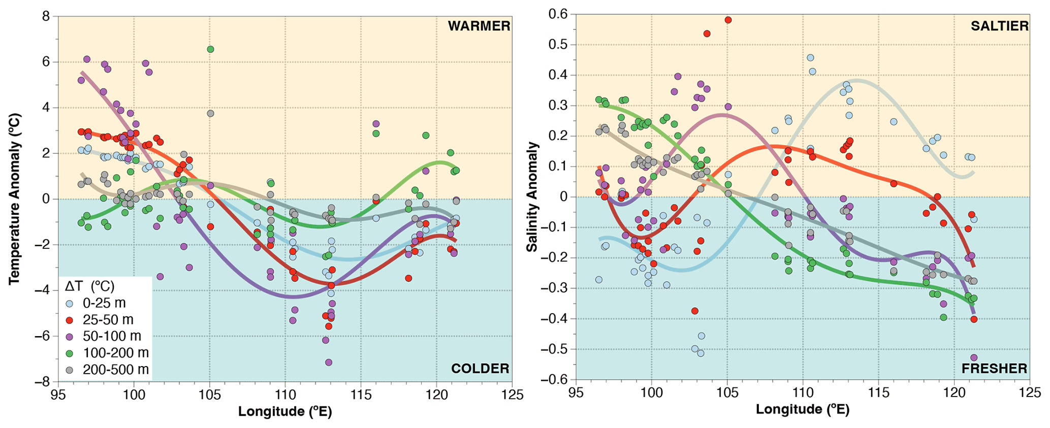
Figure A1Longitudinal distribution of temperature and salinity anomalies across the upper 500 m of water column. Anomalies are calculated by subtracting the mean of all sites for a given depth interval (e.g., 0–25, 25–50 m) from the data of a station for the same depth interval. Positive (negative) values are centered off Sumatra (off Java) showing a strong zonal trend. The largest temperature change occurs at 50–100 m, roughly corresponding to the depth of the thermocline.
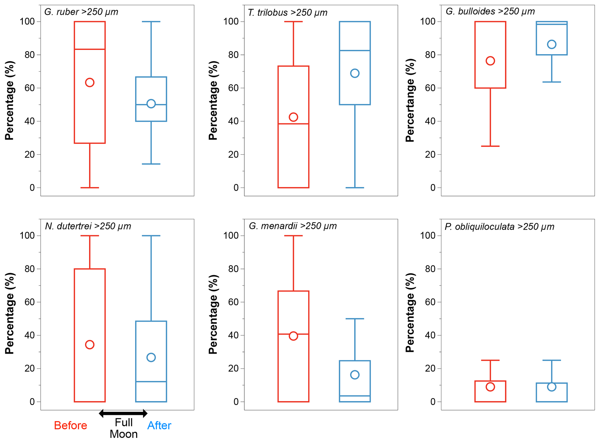
Figure A2Size class distribution (>250 µm) of the six selected species. Globigerinoides ruber, N. dutertrei, and G. menardii show a reduction in the proportion of the size class >250 µm after a full moon (blue). The large difference in their median values points to an over-representation of the large size classes suggesting synchronized reproduction; P. obliquiloculata shows no differences in the size class distribution before (red) and after (blue) the full moon; Globigerina bulloides and T. trilobus show an increase in the proportion of larger organisms after the full moon. Median values are shown by bars, and circles represent mean values.
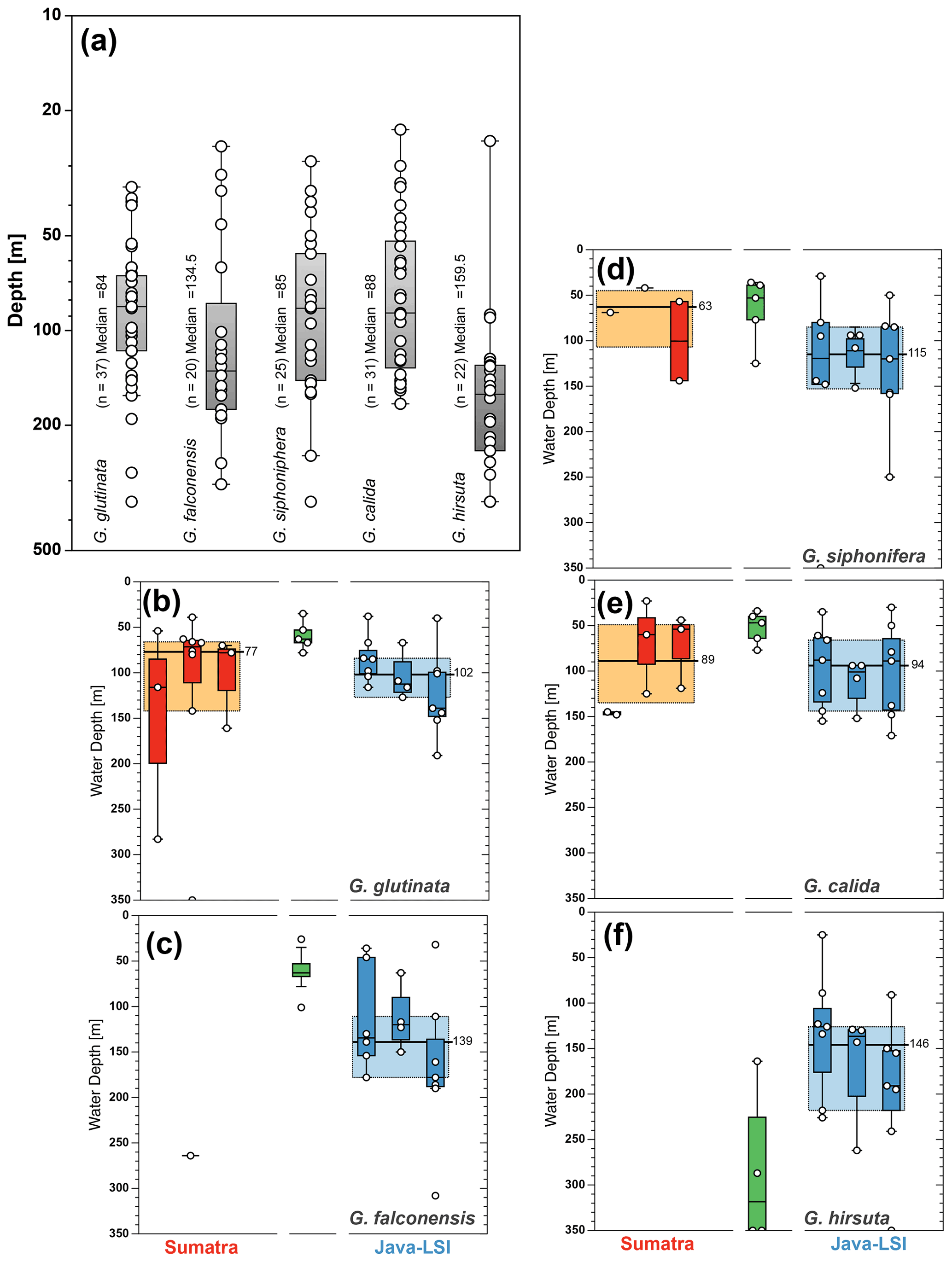
Figure A3In addition to species with paleoceanographic relevance, we calculated the (a) ALD for the species G. glutinata (84 m), G. falconensis (135 m), G. siphonifera (85 m), G. calida (88 m), and G. hirsuta (160 m). The zonal comparison of these species (b–f) is only possible for three species; G. calida shows the smallest change in ALD (∼5 m), while G. glutinata and G. siphonifera show a change of 30 and 50 m in their habitat depth between sectors. The yellow and light-blue boxes depict the first and third quartiles of the ALD values off Sumatra (non-upwelling) and off Java–LSI (upwelling). Black bars and numbers depict the median value per sector.
Table A1Details of the plankton net stations (location, water depth, and sampling date) during cruise SO-184 (Hebbeln and cruise participants, 2006). The stations are divided into seven transects. Relevant environmental parameters during the sampling include the thermal mixed-layer depth (MLDTEMP), barrier layer thickness (BL), stratification index (SI0–200), observed sea surface temperature (SST), sea surface salinity (SSS), and in situ chlorophyll a (chl a) at the surface (0–25 m) and thermocline level (100–200 m) (Table 5.1 in Hebbeln and cruise participants, 2006). Sampling gear: MultiNet (Mn), rosette sampler (Rs). NA: no data available.

Data generated in this study are available in the Supplement and on the PANGAEA database (https://doi.org/10.1594/PANGAEA.941895; Tapia, 2022).
The supplement related to this article is available online at: https://doi.org/10.5194/bg-19-3185-2022-supplement.
MM and SLH conceptualized this study. MM was responsible for the collection of planktic foraminifera and oceanographic data. RT analyzed the planktic foraminifera fauna. JG provided support for taxonomic identification. HYW contributed to the statistical analyses. The manuscript was written by RT and SLH with contributions from all co-authors, who approved its final version.
The contact author has declared that none of the authors has any competing interests.
Publisher's note: Copernicus Publications remains neutral with regard to jurisdictional claims in published maps and institutional affiliations.
This study was funded by DFG grant HE3412/15-1 (MM) and NTU Core Research Team fund 109L892604 and 110L890705 (Sze Ling Ho). Raúl Tapia acknowledges funding by MOST grants 108-2116-M-002-008, 109-2116-M-002-014, and 110-2116-M-002-007. We thank the crew and scientists participating in the PABESIA cruise (SO-184). We are grateful to Takuya Sagawa (Kanazawa University) and Yoshimi Kubota (National Science Museum) for providing a copy of the paper by Ujiié (1968) stored at the National Museum of Nature and Science in Tokyo, Japan. The manuscript benefited from the constructive comments of three anonymous reviewers.
This research has been supported by the Deutsche Forschungsgemeinschaft (grant no. HE3412/15-1); the National Taiwan University (Core Research Team 109L892604 and Core Research Team 110L890705); and the Ministry of Science and Technology, Taiwan (grant nos. 108-2116-M-002-008, 109-2116-M-002-014, and 110-2116-M-002-007).
This paper was edited by Hiroshi Kitazato and reviewed by three anonymous referees.
Anderson, O. R., Spindler, M., Bé, A. W. H., and Hemleben, C.: Trophic activity of planktonic foraminifera, J. Mar. Biol. Assoc. UK, 59, 791–799, https://doi.org/10.1017/S002531540004577X, 1979.
Aurahs, R., Grimm, G. W., Hemleben, V., Hemleben, C., and Kucera, M.: Geographical distribution of cryptic genetic types in the planktonic foraminifer Globigerinoides ruber., Mol. Ecol., 18, 1692–1706, https://doi.org/10.1111/j.1365-294X.2009.04136.x, 2009.
Bé, A. W. H.: An ecological, zoogeographic and taxonomic review of recent planktonic foraminifer, in: Oceanic Micropaleontology, edited by: Ramsay, A. T. S., Academic Press, London, 1–100, 1977.
Bé, A. W. H. and Hamlin, W. H.: Ecology of Recent Planktonic Foraminifera: Part 3: Distribution in the North Atlantic during the Summer of 1962, Micropaleontology, 13, 87, https://doi.org/10.2307/1484808, 1967.
Bé, A. W. H., Caron, D. A., and Anderson, O. R.: Effects of feeding frequency on life processes of the planktonic foraminifer Globigerinoides sacculifer in laboratory culture, J. Mar. Biol. Assoc. UK, 61, 257–277, https://doi.org/10.1017/S002531540004604X, 1981.
Bemis, B. E., Spero, H. J., Bijma, J., and Lea, D. W.: Reevaluation of the oxygen isotopic composition of planktonic foraminifera: Experimental results and revised paleotemperature equations, Paleoceanography, 13, 150–160, https://doi.org/10.1029/98PA00070, 1998.
Birch, H., Coxall, H. K., Pearson, P. N., Kroon, D., and O'Regan, M.: Planktonic foraminifera stable isotopes and water column structure: Disentangling ecological signals, Mar. Micropaleontol., 101, 127–145, https://doi.org/10.1016/j.marmicro.2013.02.002, 2013.
Brock, J. C., McClain, C. R., Anderson, D. M., Prell, W. L., and Hay, W. W.: Southwest monsoon circulation and environments of recent planktonic foraminifera in the northwestern arabian sea, Paleoceanography, 7, 799–813, https://doi.org/10.1029/92PA01267, 1992.
Caley, T., Giraudeau, J., Malaizé, B., Rossignol, L., and Pierre, C.: Agulhas leakage as a key process in the modes of Quaternary climate changes, P. Natl. Acad. Sci. USA, 109, 6835–6839, https://doi.org/10.1073/pnas.1115545109, 2012.
Caron, D. A., Bé, A. W. H., and Anderson, O. R.: Effects of variations in light intensity on life processes of the planktonic foraminifer Globigerinoides sacculifer in laboratory culture, J. Mar. Biol. Assoc. UK, 62, 435–451, https://doi.org/10.1017/S0025315400057374, 1982.
Cayre, O., Beaufort, L., and Vincent, E.: Paleoproductivity in the Equatorial Indian Ocean for the last 260 000 yr: A transfer function based on planktonic foraminifera, Quaternary Sci. Rev., 18, 839–857, https://doi.org/10.1016/S0277-3791(98)00036-5, 1999.
CLIMAP Project Members: The surface of the ice-age Earth, Science, 191, 1131–1137, https://doi.org/10.1126/science.191.4232.1131, 1976.
Conan, S. M. H. and Brummer, G. J. A.: Fluxes of planktic foraminifera in response to monsoonal upwelling on the Somalia Basin margin, Deep-Sea Res. Pt. II, 47, 2207–2227, https://doi.org/10.1016/S0967-0645(00)00022-9, 2000.
Dang, H., Jian, Z., Wang, Y., Mohtadi, M., Rosenthal, Y., Ye, L., Bassinot, F., and Kuhnt, W.: Pacific warm pool subsurface heat sequestration modulated Walker circulation and ENSO activity during the Holocene, Sci. Adv., 6, 42, https://doi.org/10.1126/sciadv.abc0402, 2020.
Davis, C. V., Wishner, K., Renema, W., and Hull, P. M.: Vertical distribution of planktic foraminifera through an oxygen minimum zone: how assemblages and test morphology reflect oxygen concentrations, Biogeosciences, 18, 977–992, https://doi.org/10.5194/bg-18-977-2021, 2021.
de Boyer Montégut, C., Madec, G., Fischer, A. S., Lazar, A., and Ludicone, D.: Mixed layer depth over the global ocean: An examination of profile data and a profile-based climatology, J. Geophys. Res., 109, C12003, https://doi.org/10.1029/2004JC002378, 2004.
Ding, X., Bassinot, F., Guichard, F., Li, Q. Y., Fang, N. Q., Labeyrie, L., Xin, R. C., Adisaputra, M. K., and Hardjawidjaksana, K.: Distribution and ecology of planktonic foraminifera from the seas around the Indonesian Archipelago, Mar. Micropaleontol., 58, 114–134, https://doi.org/10.1016/j.marmicro.2005.10.003, 2006.
Ding, X., Bassinot, F., Guichard, F., and Fang, N. Q.: Indonesian Throughflow and monsoon activity records in the Timor Sea since the last glacial maximum, Mar. Micropaleontol., 101, 115–126, https://doi.org/10.1016/j.marmicro.2013.02.003, 2013.
Du, Y. and Zhang, Y.: Satellite and Argo Observed Surface Salinity Variations in the Tropical Indian Ocean and Their Association with the Indian Ocean Dipole Mode, J. Climate, 28, 695–713, https://doi.org/10.1175/JCLI-D-14-00435.1, 2015.
Duplessy, J. C., Bé, A. W. H., and Blanc, P. L.: Oxygen and carbon isotopic composition and biogeographic distribution of planktonic foraminifera in the Indian Ocean, Palaeogeogr. Palaeocl., 33, 9–46, https://doi.org/10.1016/0031-0182(81)90031-6, 1981.
Eguchi, N. O., Kawahata, H., and Taira, A.: Seasonal response of planktonic foraminifera to surface ocean condition: Sediment trap results from the central North Pacific Ocean, J. Oceanogr., 55, 681–691, 1999.
Fairbanks, R. G., Wiebe, P. H., and Bé, A. W.: Vertical distribution and isotopic composition of living planktonic foraminifera in the Western north Atlantic, Science, 207, 61–63, https://doi.org/10.1126/science.207.4426.61, 1980.
Fan, W., Jian, Z., Chu, Z., Dang, H., Wang, Y., Bassinot, F., Han, X., and Bian, Y.: Variability of the Indonesian Throughflow in the Makassar Strait over the last 30 ka, Sci. Rep., 8, 5678, https://doi.org/10.1038/s41598-018-24055-1, 2018.
Farmer, E. J., Chapman, M. R., and Andrews, J. E.: Holocene temperature evolution of the subpolar North Atlantic recorded in the ratios of surface and thermocline dwelling planktonic foraminifers, Global Planet. Change, 79, 234–243, https://doi.org/10.1016/j.gloplacha.2011.02.003, 2011.
Faul, K. L.: Reconstructions of upwelling, productivity, and photic zone depth in the eastern equatorial pacific ocean using planktonic foraminiferal stable isotopes and abundances, J. Foramin. Res., 30, 110–125, https://doi.org/10.2113/0300110, 2000.
Field, D. B.: Variability in vertical distributions of planktonic foraminifera in the California Current: Relationships to vertical ocean structure, Paleoceanography, 19, PA2014, https://doi.org/10.1029/2003PA000970, 2004.
Gordon, A. L.: Oceanography of the indonesian seas and their throughflow, Oceanography, 18, 14–27, https://doi.org/10.5670/oceanog.2005.01, 2005.
Gordon, A. L. and Fine, R. A.: Pathways of water between the Pacific and the Indonesian seas, Nature, 379, 146–149, 1996.
Greco, M., Jonkers, L., Kretschmer, K., Bijma, J., and Kucera, M.: Depth habitat of the planktonic foraminifera Neogloboquadrina pachyderma in the northern high latitudes explained by sea-ice and chlorophyll concentrations, Biogeosciences, 16, 3425–3437, https://doi.org/10.5194/bg-16-3425-2019, 2019.
Groeneveld, J. and Chiessi, C. M.: of Globorotalia inflata as a recorder of permanent thermocline temperatures in the South Atlantic, Paleoceanography, 26, PA2203, https://doi.org/10.1029/2010PA001940, 2011.
Hebbeln, D. and cruise participants: Report and preliminary results of the RV SONNE Cruise SO-184, Pabesia, Durban (South Africa)–Cilacap (Indonesia)–Darwin (Australia), 8 July–13 September 2005, https://media.suub.uni-bremen.de/handle/elib/3657 (last access: 4 July 2022), 2006.
Hemleben, C., Spindler, M., and Anderson, O. R.: Modern Planktonic Foraminifera, Springer, New York, NY, https://doi.org/10.1007/978-1-4612-3544-6_1, 1989.
Hollstein, M., Mohtadi, M., Rosenthal, Y., Moffa Sanchez, P., Oppo, D., Martínez Méndez, G., Steinke, S., and Hebbeln, D.: Stable oxygen isotopes and mg/ca in planktic foraminifera from modern surface sediments of the western pacific warm pool: implications for thermocline reconstructions, Paleoceanography, 32, 1174–1194, https://doi.org/10.1002/2017PA003122, 2017.
Imbrie, J. and Kipp, N. G.: A new micropaleontological method for quantitative paleoclimatology: Application to a Late Pleistocene Caribbean core, in: The Late Cenozoic Glacial Ages, edited by: Turekian, K., Yale Univ. Press, New Haven, Conn., 71–81, 1971.
Jonkers, L., Hillebrand, H., and Kucera, M.: Global change drives modern plankton communities away from the pre-industrial state, Nature, 570, 372–375, https://doi.org/10.1038/s41586-019-1230-3, 2019.
Jorissen, F. J., de Stigter, H. C., and Widmark, J. G. V.: A conceptual model explaining benthic foraminiferal microhabitats, Mar. Micropaleontol., 26, 3–15, https://doi.org/10.1016/0377-8398(95)00047-X, 1995.
Kara, A. B., Rochford, P. A., and Hurlburt, H. E.: An optimal definition for ocean mixed layer depth, J. Geophys. Res., 105, 16803–16821, https://doi.org/10.1029/2000JC900072, 2000.
Karas, C., Nürnberg, D., Tiedemann, R., and Garbe-Schönberg, D.: Pliocene Indonesian Throughflow and Leeuwin Current dynamics: Implications for Indian Ocean polar heat flux, Paleoceanography, 26, PA2217, https://doi.org/10.1029/2010PA001949, 2011.
Katz, M. E., Cramer, B. S., Franzese, A., Honisch, B., Miller, K. G., Rosenthal, Y., and Wright, J. D.: Traditional and emerging geochemical proxies in foraminifera, J. Foramin. Res., 40, 165–192, https://doi.org/10.2113/gsjfr.40.2.165, 2010.
Kemle-von Mücke, S. and Oberhänsli, H.: The distribution of living planktic foraminifera in relation to southeast atlantic oceanography, in: Use of proxies in Paleoceanography, edited by: Fischer, G. and Wefer, G., Springer, Berlin, Heidelberg, 91–115, https://doi.org/10.1007/978-3-642-58646-0_3, 1999.
Kennett, J. P. and Srinivasan, M. S.: Neogene planktonic foraminifera: A phylogenetic atlas, Hutchinson Ross Publishing Company, Stroudsburg, Pa., ISBN 0-87933-070-8, 1983.
Kimoto, K.: Planktic Foraminifera, in: Marine Protists, edited by: Ohtsuka, S., Suzaki, T., Horiguchi, T., Suzuki, N., and Not, F., Springer Japan, Tokyo, 129–178, https://doi.org/10.1007/978-4-431-55130-0_7, 2015.
Kucera, M.: Planktonic foraminifera as tracers of past oceanic environments, in: Proxies in late cenozoic paleoceanography, vol. 1, Elsevier, 213–262, https://doi.org/10.1016/S1572-5480(07)01011-1, 2007.
Kucera, M.: Determination of past sea surface temperatures, in: Encyclopedia of ocean sciences, Elsevier, 98–113, https://doi.org/10.1016/B978-012374473-9.00700-1, 2009.
Kuroyanagi, A. and Kawahata, H.: Vertical distribution of living planktonic foraminifera in the seas around Japan, Mar. Micropaleontol., 53, 173–196, https://doi.org/10.1016/j.marmicro.2004.06.001, 2004.
Lea, D. W.: Elemental and isotopic proxies of past ocean temperatures, in: Treatise on Geochemistry, Elsevier, 373–397, https://doi.org/10.1016/B978-0-08-095975-7.00614-8, 2014.
Lessa, D., Morard, R., Jonkers, L., Venancio, I. M., Reuter, R., Baumeister, A., Albuquerque, A. L., and Kucera, M.: Distribution of planktonic foraminifera in the subtropical South Atlantic: depth hierarchy of controlling factors, Biogeosciences, 17, 4313–4342, https://doi.org/10.5194/bg-17-4313-2020, 2020.
Locarnini, R. A., Mishonov, A. V., Baranova, O. K., Boyer, T. P., Zweng, M. M., Garcia, H. E., Reagan, J. R., Seidov, D., Weathers, K., Paver, C. R., and Smolyar, I.: World Ocean Atlas 2018, Vol. 1: Temperature, edited by: Mishonov, A., NOAA Atlas NESDIS 81, http://www.nodc.noaa.gov/OC5/indprod.html (last access: 4 July 2022), 2018.
Manly, B. F. J.: Randomization, bootstrap and monte carlo methods in biology, 2rd edn., Chapman and Hall/CRC, ISBN 0412721309, 1997.
Marchant, M., Hebbeln, D., Giglio, S., Coloma, C., and González, H. E.: Seasonal and interannual variability in the flux of planktic foraminifera in the Humboldt Current System off central Chile (30∘ S), Deep-Sea Res. Pt. II, 51, 2441–2455, https://doi.org/10.1016/j.dsr2.2004.08.013, 2004.
Meilland, J., Siccha, M., Weinkauf, M. F. G., Jonkers, L., Morard, R., Baranowski, U., Baumeister, A., Bertlich, J., Brummer, G.-J., Debray, P., Fritz-Endres, T., Groeneveld, J., Magerl, L., Munz, P., Rillo, M. C., Schmidt, C., Takagi, H., Theara, G., and Kucera, M.: Highly replicated sampling reveals no diurnal vertical migration but stable species-specific vertical habitats in planktonic foraminifera, J. Plankton Res., 41, 127–141, https://doi.org/10.1093/plankt/fbz002, 2019.
Mohtadi, M., Max, L., Hebbeln, D., Baumgart, A., Krück, N., and Jennerjahn, T.: Modern environmental conditions recorded in surface sediment samples off W and SW Indonesia: Planktonic foraminifera and biogenic compounds analyses, Mar. Micropaleontol., 65, 96–112, https://doi.org/10.1016/j.marmicro.2007.06.004, 2007.
Mohtadi, M., Steinke, S., Groeneveld, J., Fink, H. G., Rixen, T., Hebbeln, D., Donner, B., and Herunadi, B.: Low-latitude control on seasonal and interannual changes in planktonic foraminiferal flux and shell geochemistry off south Java: A sediment trap study, Paleoceanography, 24, PA1201, https://doi.org/10.1029/2008PA001636, 2009.
Mohtadi, M., Oppo, D. W., Lückge, A., DePol-Holz, R., Steinke, S., Groeneveld, J., Hemme, N., and Hebbeln, D.: Reconstructing the thermal structure of the upper ocean: Insights from planktic foraminifera shell chemistry and alkenones in modern sediments of the tropical eastern Indian Ocean, Paleoceanography, 26, PA3219, https://doi.org/10.1029/2011PA002132, 2011.
Mohtadi, M., Prange, M., Oppo, D. W., De Pol-Holz, R., Merkel, U., Zhang, X., Steinke, S., and Lückge, A.: North Atlantic forcing of tropical Indian Ocean climate, Nature, 509, 76–80, https://doi.org/10.1038/nature13196, 2014.
Mohtadi, M., Prange, M., Schefuß, E., and Jennerjahn, T. C.: Late Holocene slowdown of the Indian Ocean Walker circulation, Nat. Commun., 8, 1015, https://doi.org/10.1038/s41467-017-00855-3, 2017.
Murray, J.: On the distribution of the pelagic foraminifera at the surface and on the floor of the ocean, Sci. Am., 44, 18026–18028, https://doi.org/10.1038/scientificamerican08141897-18026supp, 1897.
Muskananfola, M. R., Jumsar, and Wirasatriya, A.: Spatio-temporal distribution of chlorophyll a concentration, sea surface temperature and wind speed using aqua-modis satellite imagery over the Savu Sea, Indonesia, Remote Sensing Applications: Society and Environment, 22, 100483, https://doi.org/10.1016/j.rsase.2021.100483, 2021.
Ortiz, J. D. and Mix, A. C.: Comparison of Imbrie-Kipp Transfer Function and modern analog temperature estimates using sediment trap and core top foraminiferal faunas, Paleoceanography, 12, 175–190, https://doi.org/10.1029/96PA02878, 1997.
Pang, X., Bassinot, F., and Sepulcre, S.: Indonesian Throughflow variability over the last two glacial-interglacial cycles: Evidence from the eastern Indian Ocean, Quaternary Sci. Rev., 256, 106839, https://doi.org/10.1016/j.quascirev.2021.106839, 2021.
Parker, F. L.: Planktonic foraminiferal species in pacific sediments, Micropaleontology, 8, 219, https://doi.org/10.2307/1484745, 1962.
Pécseli, H. L., Trulsen, J. K., and Fiksen, Ø.: Predator-prey encounter and capture rates in turbulent environments, Limnol. Oceanogr., 4, 85–105, https://doi.org/10.1215/21573689-2768717, 2014.
Peeters, F. J. C. and Brummer, G.-J. A.: The seasonal and vertical distribution of living planktic foraminifera in the NW Arabian Sea, Geological Society, London, Special Publications, 195, 463–497, https://doi.org/10.1144/GSL.SP.2002.195.01.26, 2002.
Peterson, W.: Life cycle strategies of copepods in coastal upwelling zones, J. Marine Syst., 15, 313–326, https://doi.org/10.1016/S0924-7963(97)00082-1, 1998.
Peterson, W. T., Miller, C. B., and Hutchinson, A.: Zonation and maintenance of copepod populations in the Oregon upwelling zone, Deep-Sea Res., 26, 467–494, https://doi.org/10.1016/0198-0149(79)90091-8, 1979.
Qu, T. and Meyers, G.: Seasonal variation of barrier layer in the southeastern tropical Indian Ocean, J. Geophys. Res., 110, C11003, https://doi.org/10.1029/2004JC002816, 2005.
Qu, T., Du, Y., Stachan, J., Meyers, G., and Slingo, J.: Sea surface temperature and its variability in the indonesian region, Oceanography, 18, 50–61, https://doi.org/10.5670/oceanog.2005.05, 2005.
R Core Team: R: A language and environment for statistical computing, Computer software, R Foundation for Statistical Computing, Vienna, Austria, 2021.
Rebotim, A., Voelker, A. H. L., Jonkers, L., Waniek, J. J., Meggers, H., Schiebel, R., Fraile, I., Schulz, M., and Kucera, M.: Factors controlling the depth habitat of planktonic foraminifera in the subtropical eastern North Atlantic, Biogeosciences, 14, 827–859, https://doi.org/10.5194/bg-14-827-2017, 2017.
Regenberg, M., Regenberg, A., Garbe-Schönberg, D., and Lea, D. W.: Global dissolution effects on planktonic foraminiferal ratios controlled by the calcite-saturation state of bottom waters, Paleoceanography, 29, 127–142, https://doi.org/10.1002/2013PA002492, 2014.
Sautter, L. R. and Sancetta, C.: Seasonal associations of phytoplankton and planktic foraminifera in an upwelling region and their contribution to the seafloor, Mar. Micropaleontol., 18, 263–278, https://doi.org/10.1016/0377-8398(92)90043-J, 1992.
Sautter, L. R. and Thunell, R. C.: Seasonal Variability in the δ18O and δ13C of Planktonic Foraminifera from an Upwelling Environment: Sediment Trap Results from the San Pedro Basin, Southern California Bight, Paleoceanography, 6, 307–334, https://doi.org/10.1029/91PA00385, 1991.
Schiebel, R. and Hemleben, C.: Modern planktic foraminifera, Palaeontol. Z., 79, 135–148, https://doi.org/10.1007/BF03021758, 2005.
Schiebel, R. and Hemleben, C.: Planktic foraminifers in the modern ocean, 2d edn., Springer, Berlin, Heidelberg, 2017.
Schiebel, R., Waniek, J., Bork, M., and Hemleben, C.: Planktic foraminiferal production stimulated by chlorophyll redistribution and entrainment of nutrients, Deep-Sea Res. Pt. I, 48, 721–740, https://doi.org/10.1016/S0967-0637(00)00065-0, 2001.
Schiebel, R., Spielhagen, R. F., Garnier, J., Hagemann, J., Howa, H., Jentzen, A., Martínez-Garcia, A., Meilland, J., Michel, E., Repschläger, J., Salter, I., Yamasaki, M., and Haug, G.: Modern planktic foraminifers in the high-latitude ocean, Mar. Micropaleontol., 136, 1–13, https://doi.org/10.1016/j.marmicro.2017.08.004, 2017.
Schiebel, R., Smart, S. M., Jentzen, A., Jonkers, L., Morard, R., Meilland, J., Michel, E., Coxall, H. K., Hull, P. M., de Garidel-Thoron, T., Aze, T., Quillévéré, F., Ren, H., Sigman, D. M., Vonhof, H. B., Martínez-García, A., Kučera, M., Bijma, J., Spero, H. J., and Haug, G. H.: Advances in planktonic foraminifer research: New perspectives for paleoceanography, Revue de Micropaléontologie, 61, 113–138, https://doi.org/10.1016/j.revmic.2018.10.001, 2018.
Schlitzer, R.: Ocean Data View, Computer software, https://odv.awi.de (last access: 14 October 2021), 2021.
Smith, R. A., Castañeda, I. S., Groeneveld, J., De Vleeschouwer, D., Henderiks, J., Christensen, B. A., Renema, W., Auer, G., Bogus, K., Gallagher, S. J., and Fulthorpe, C. S.: Plio-pleistocene indonesian throughflow variability drove eastern indian ocean sea surface temperatures, Paleoceanography and Paleoclimatology, 35, e2020PA003872, https://doi.org/10.1029/2020PA003872, 2020.
Somavilla, R., González-Pola, C., and Fernández-Diaz, J.: The warmer the ocean surface, the shallower the mixed layer. How much of this is true?, J. Geophys. Res.-Oceans, 122, 7698–7716, https://doi.org/10.1002/2017JC013125, 2017.
Spezzaferri, S., Kucera, M., Pearson, P. N., Wade, B. S., Rappo, S., Poole, C. R., Morard, R., and Stalder, C.: Fossil and genetic evidence for the polyphyletic nature of the planktonic foraminifera “Globigerinoides”, and description of the new genus Trilobatus, PLoS ONE, 10, e0128108, https://doi.org/10.1371/journal.pone.0128108, 2015.
Sprintall, J. and Révelard, A.: The Indonesian Throughflow response to Indo-Pacific climate variability, J. Geophys. Res.-Oceans, 119, 1161–1175, https://doi.org/10.1002/2013JC009533, 2014.
Steinke, S., Prange, M., Feist, C., Groeneveld, J., and Mohtadi, M.: Upwelling variability off southern Indonesia over the past two millennia, Geophys. Res. Lett., 41, 7684–7693, https://doi.org/10.1002/2014GL061450, 2014.
Steph, S., Regenberg, M., Tiedemann, R., Mulitza, S., and Nürnberg, D.: Stable isotopes of planktonic foraminifera from tropical Atlantic/Caribbean core-tops: Implications for reconstructing upper ocean stratification, Mar. Micropaleontol., 71, 1–19, https://doi.org/10.1016/j.marmicro.2008.12.004, 2009.
Susanto, R. D. and Marra, J.: Effect of the 1997/98 el niño on chlorophyll a variability along the southern coasts of java and sumatra, Oceanography, 18, 124–127, https://doi.org/10.5670/oceanog.2005.13, 2005.
Susanto, R. D., Gordon, A. L., and Zheng, Q.: Upwelling along the coasts of Java and Sumatra and its relation to ENSO, Geophys. Res. Lett., 28, 1599–1602, https://doi.org/10.1029/2000GL011844, 2001.
Susanto, R. D., Moore, T. S., and Marra, J.: Ocean color variability in the Indonesian Seas during the SeaWiFS era, Geochem. Geophy. Geosy., 7, Q05021, https://doi.org/10.1029/2005GC001009, 2006.
Takagi, H., Kimoto, K., Fujiki, T., and Moriya, K.: Effect of nutritional condition on photosymbiotic consortium of cultured Globigerinoides sacculifer (Rhizaria, Foraminifera), Symbiosis, 76, 25–39, https://doi.org/10.1007/s13199-017-0530-3, 2018.
Tapia, R., Nürnberg, D., Ronge, T., and Tiedemann, R.: Disparities in glacial advection of Southern Ocean Intermediate Water to the South Pacific Gyre, Earth Planet. Sc. Lett., 410, 152–164, https://doi.org/10.1016/j.epsl.2014.11.031, 2015.
Tapia, R., Nürnberg, D., Ho, S. L., Lamy, F., Ullermann, J., Gersonde, R., and Tiedemann, R.: Glacial differences of Southern Ocean Intermediate Waters in the Central South Pacific, Quaternary Sci. Rev., 208, 105–117, https://doi.org/10.1016/j.quascirev.2019.01.016, 2019.
Tapia, R.: Contrasting vertical distributions of recent planktic foraminifera off Indonesia during the southeast monsoon: implications for paleoceanographic reconstructions, PANGAEA [data set], https://doi.org/10.1594/PANGAEA.941895, 2022.
Tillinger, D.: Physical oceanography of the present day Indonesian Throughflow, Geological Society, London, Special Publications, 355, 267–281, https://doi.org/10.1144/SP355.13, 2011.
Tolderlund, D. S. and Bé, A. W. H.: Seasonal distribution of planktonic foraminifera in the western north atlantic, Micropaleontology, 17, 297, https://doi.org/10.2307/1485143, 1971.
Ujiié, H.: Distribution of living planktonic foraminifera in the southeast Indian Ocean, Bull. Nat. Sci. Mus. Tokyo, 11, 97–125, 1968.
Verheye, H. M., Hutchings, L., and Peterson, W. T.: Life history and population maintenance strategies of Calanoides carinatus (Copepoda: Calanoida) in the southern Benguela ecosystem, S. Afr. J. Marine Sci., 11, 179–191, https://doi.org/10.2989/025776191784287600, 1991.
Wang, L.: Isotopic signals in two morphotypes of Globigerinoides ruber (white) from the South China Sea: implications for monsoon climate change during the last glacial cycle, Palaeogeogr. Palaeocl., 161, 381–394, https://doi.org/10.1016/S0031-0182(00)00094-8, 2000.
Wang, X., Jian, Z., Lückge, A., Wang, Y., Dang, H., and Mohtadi, M.: Precession-paced thermocline water temperature changes in response to upwelling conditions off southern Sumatra over the past 300 000 years, Quaternary Sci. Rev., 192, 123–134, https://doi.org/10.1016/j.quascirev.2018.05.035, 2018.