the Creative Commons Attribution 4.0 License.
the Creative Commons Attribution 4.0 License.
 | 20 Jan 2022
Investigating controls of shell growth features in a foundation bivalve species: seasonal trends and decadal changes in the California mussel
Veronica Padilla Vriesman
Sandra J. Carlson
Tessa M. Hill
Marine bivalve mollusk shells can offer valuable insights into past oceanographic variability and seasonality. Given its ecological and archeological significance, Mytilus californianus (California mussel) presents the opportunity to examine seasonal and decadal changes recorded in its shell over centuries to millennia. While dark–light growth bands in M. californianus shells could be advantageous for reconstructing past environments, uncertainties remain regarding shell structure, environmental controls of dark–light-band formation, and the amount of time represented by a dark–light pair. By analyzing a suite of M. californianus shells collected in 2002, 2003, 2019, and 2020 from Bodega Bay, California, we describe the mineralogical composition; establish relationships among the growth band pattern, micro-environment, and collection season; and compare shell structure and growth band expression between the archival (2002–2003) and modern (2019–2020) shells. We identified three mineralogical layers in M. californianus: an outer prismatic calcite layer, a middle aragonite layer, and a secondary inner prismatic calcite layer, which makes M. californianus the only Mytilus species to precipitate a secondary calcite layer. Within the inner calcite layer, light bands are strongly correlated with winter collection months and could be used to reconstruct periods with moderate, stable temperatures and minimal upwelling. Additionally, modern shells have significantly thinner inner calcite layers and more poorly expressed growth bands than the archival shells, although we also show that growth band contrast is strongly influenced by the micro-environment. Mytilus californianus from northern California is calcifying differently, and apparently more slowly, than it was 20 years ago.
- Article
(4647 KB) - Full-text XML
-
Supplement
(2591 KB) - BibTeX
- EndNote


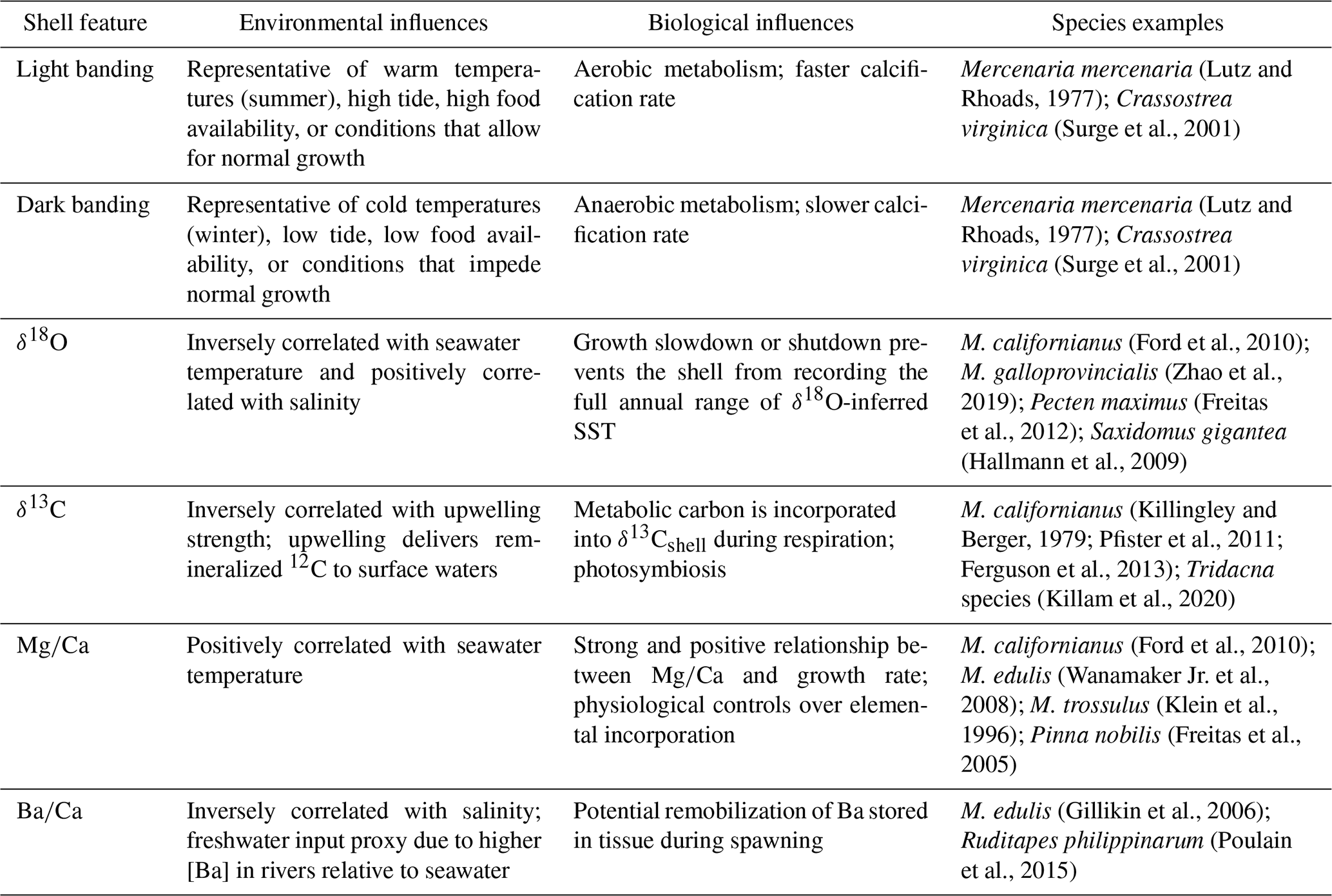
Marine bivalve shells offer a complex yet valuable record to explore questions about paleo- and modern seasonal extremes, since many bivalve species can record ambient conditions as they calcify (Jones and Quitmyer, 1996; Wanamaker Jr. et al., 2006; Welsh et al., 2011; Schöne and Gillikin, 2013; Trofimova et al., 2021). Detailed paleoenvironmental, paleoceanographic, and anthropological information can be extracted from shell growth records over multiple timescales depending on the species' shell growth rate, the accuracy of ontogenetic age estimates, and the periodicity of the growth band pattern within the shell (Hallmann et al., 2013; Jazwa and Kennett, 2016; Cannon and Burchell, 2017). Seasonally resolved shell growth features allow for the approximation of historic baselines of temperature variability, the comparison of inferred paleotemperature extremes to modern temperature ranges, and the prediction of climatic changes on organisms and ecosystems, which are typically controlled more strongly by extremes (Sydeman et al., 2014; Poloczanska et al., 2016; Mellin et al., 2016) than they are by average conditions. During calcification, both environmental and biological factors influence shell characteristics and chemistry differently depending on the species (Table 1). Light bands in bivalve shells represent increments of normal growth, while dark bands indicate slow or stunted growth during periods of stressful or sub-optimal conditions (Lutz and Rhoads, 1977; Killam and Clapham, 2018). Dark banding is possibly the product of increased organic material relative to calcium carbonate production during anaerobic conditions or the visual representation of changes to the crystal microfabric when calcification occurs more slowly. In either case, however, dark bands are associated with reduced calcification. Using this relationship, we aim to link environmental conditions with growth band coloration to investigate the timing and periodicity of dark–light-band formation in marine mussel shells from northern California and determine whether there are spatial or temporal differences in growth patterns. In order to interpret the shell growth features of a particular species as a paleoseasonal or paleoceanographic archive, a clear understanding of the environmental parameters influencing the appearance of the growth band pattern and the timing of shell growth is required. For example, the well-studied bivalve species Arctica islandica has served as a reliable climate record with sub-seasonal resolution for high-latitude marine environments because it has been determined to be long-lived (∼ 500 or more years) (Butler et al., 2013). Schöne et al. (2005a) and Schöne (2013) concluded that A. islandica produces annual and daily growth lines that form continually throughout the year. One individual provides high-resolution environmental information and seasonal extremes for multiple centuries within a single shell (Weidman et al., 1994; Schöne et al., 2005a; Schöne, 2013). While A. islandica is a unique archive due to its longevity and regularity, the relationships between environmental parameters and shell growth features should be tested in other, more distantly related bivalve species to optimize the paleoceanographic utility of fossil, archeological, and historic specimens.
Table 1Chemical and microstructural growth features recorded in bivalve shells and their environmental and biological influences. Species examples are not exhaustive.
Mytilus californianus as a study organism
One species of interest for the northeastern Pacific coast is Mytilus californianus (California mussel), an ecologically and culturally significant intertidal species that spans 20∘ of latitude ranging from the Aleutian Islands of Alaska to Baja California in northern Mexico (Paine, 1974). Mytilus californianus is a foundation species in rocky intertidal environments, playing a critical role in structuring and maintaining the intertidal community. It provides a habitat for ∼ 300 interstitial species, filters detritus from seawater during feeding, and serves as a food source for a variety of predators (Paine, 1974; Smith et al., 2009; Connor et al., 2016). Mytilus californianus shells are abundant in coastal California shell middens that span the terminal Pleistocene (∼ 12 000 BP) through the late Holocene in age; many Indigenous communities, including the Coast Miwok, Island Chumash, and Salinan peoples, harvested California mussels as a critical or even primary food source (Jones and Richman, 1995; Jones and Kennett 1999; Kennedy, 2004; Kennedy et al., 2005; Braje et al., 2007, 2011, 2012; Campbell and Braje, 2015). Shellfish collection remains an important element of traditional ecological knowledge and is still practiced by Indigenous communities along the west coast of North America (Lepofsky et al., 2015). Given its prevalence in the archeological record and abundance in modern intertidal ecosystems, M. californianus provides the opportunity to reconstruct coastal environments at various temporal scales and explore variation in shell growth features in a single species over the past ∼ 12 000 years from multiple northeastern Pacific coast sites. However, our understanding of shell structure and calcification rates and timing in M. californianus is highly variable and site-specific (e.g., Blanchette et al., 2007; Smith et al., 2009; Ford et al., 2010), hindering interpretations in fields ranging from archeology to paleoceanography.
In order to accurately interpret M. californianus shell growth features – and to determine whether M. californianus can serve as a reliable paleoarchive – we analyzed the shell morphology, mineralogical layering, and growth band pattern of 40 specimens collected over various seasons in 2002, 2003, 2019, and 2020 in conjunction with sea surface temperature (SST) records and upwelling indices for the same location (Bodega Bay, California, 38.3332∘ N, 123.0481∘ W). We aimed to first characterize the shell structure and mineralogical layering of M. californianus and then focused closely on the growth band pattern in order to investigate environmental controls on shell growth and address the following questions. (1) What is the influence of the micro-environment (tidal position and habitat type) on the visual expression of growth bands in M. californianus shells from Bodega Bay? (2) What is the influence of oceanographic conditions (SST and upwelling intensity) on the coloration (dark or light) of growth bands? (3) Are there temporal or periodic environmental trends (seasonal, annual, or decadal) influencing shell growth patterns (growth band expression and coloration of growth bands)?
2.1 Oceanographic setting
Bodega Bay, California, is located approximately 100 km north of San Francisco Bay in the central portion of the California Current System (CCS). Oceanographically, Bodega Bay experiences strong seasonal cycles: a spring–early-summer (March to July) upwelling season with low mean monthly SSTs (∼ 10 to 12 ∘C), a late-summer–fall relaxation season (August to November) with reduced upwelling and relatively warmer monthly SSTs (∼ 13 to 15 ∘C), and a cool winter (December through February) with heavy precipitation and moderate SSTs (García-Reyes and Largier, 2010, 2012). The CCS comprises the dominant south-flowing California Current, the subsurface north-flowing California Undercurrent, and the seasonal north-flowing Davidson Current present at the sea surface in winter (Hickey and Banas, 2003). The geometry of the California coastline interacts with the CCS to produce different temperature regimes in northern and southern California; north of Point Conception, the coastline is roughly parallel to alongshore winds, resulting in high Ekman transport and strong upwelling near the coast (Huyer, 1983; Checkley and Barth, 2009). Interannual and decadal regional variability within the CCS is largely driven by the El Niño–Southern Oscillation (ENSO) and Pacific Decadal Oscillation (PDO) (García-Reyes and Largier, 2012). In addition to ENSO and PDO phases, local-scale coastal variability on the order of meters to a few kilometers is controlled by local surface warming and wind stress (Dever and Lentz, 1994; García-Reyes and Largier, 2012).
For this study, three intertidal collection locations were chosen: Horseshoe Cove (a protected marine environment in Bodega Marine Reserve, BMR), an open-coast BMR site (350 m north of Horseshoe Cove), and a third site at Portuguese Beach (an open-coast site 7 km north of BMR). All three collection locations are located along Sonoma Coast, west and northwest of Bodega Harbor. Sonoma Coast is considered one oceanographic region, since it is part of the same upwelling cell within the CCS (Largier et al., 1993; Wing et al., 1995), and 7 km of alongshore separation results in the same coastal SST and upwelling patterns at BMR and Portuguese Beach (John Largier, personal communication, 2021).
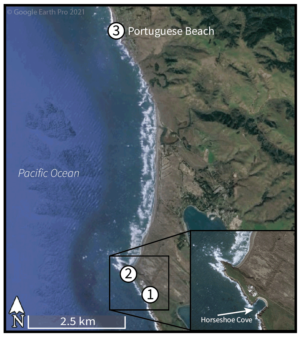
Figure 1Intertidal collection sites at Bodega Bay, California, along Sonoma Coast. Sites 1 and 2 are located within Bodega Marine Reserve, and site 3 is located at Portuguese Beach. Modern shells were collected alive in 2019 and 2020 at sites 1 and 2 (Horseshoe Cove and the open-coast site, respectively). Archival shells were collected alive 7 km north at Portuguese Beach in 2002 and 2003. © Google Earth Pro 2021.
2.2 Specimen collection and preparation
To examine the environmental and temporal factors influencing growth band patterns, we analyzed shell growth features from 40 M. californianus samples (n= 27 shells from 2019 and 2020; n= 13 shells collected in 2002 and 2003). Specimens were categorized as either modern (collected in 2019–2020) or archival (collected in 2002–2003). On 18 January 2019, nine initial M. californianus individuals were hand-collected from the intertidal zone of Horseshoe Cove (38.33325∘ N, 123.0480571∘ W) during low tide (−1.13 m) (Fig. 1) with written permission from BMR. Live specimens were collected along a 6 m transect: three specimens from the high intertidal position (HIP) 0 m from the shore, three specimens from the middle intertidal position (MIP) 3 m from the shore, and three specimens from the low intertidal position (LIP) 6 m from the shore. Specimens were immediately sacrificed by scraping soft tissue from the shells. Valves were scrubbed with hydrogen peroxide to remove epibionts, rinsed with deionized water, oven-dried at 40 ∘C for 30 min, and air-dried overnight. Additional specimen collections took place on 11 July 2019 and 6 June 2020 at BMR. As previously, shells were hand-collected by intertidal position at Horseshoe Cove and from the open-coast BMR site in order to compare shells from a variety of micro-environments: tidal position (HIP, MIP, or LIP) and habitat type (open-coast or protected). Both BMR collection sites experience marine rather than estuarine conditions; mean daily salinity at BMR was 33.4 ± 0.34 (1 SD) PSU (practical salinity unit) in 2018.
Additionally, 13 archival M. californianus shells live-collected at Portuguese Beach on 10 May 2002, 19 July 2002, 1 December 2002, 23 December 2002, and 7 September 2003 were included for temporal comparisons. Portuguese Beach is an open-coast, rocky intertidal site ∼ 7 km north of the BMR collection locations. All 13 Portuguese Beach specimens were collected from the MIP by Michael A. Kennedy for dissertation research with the Department of Anthropology of the University of California, Davis (Kennedy, 2004).

Figure 2Anatomy of M. californianus whole valve and cross section. (a) Line drawing of whole valve showing where shell length was measured. Red dashed line denotes maximum growth axis along which the valve was cut to prepare a thin section. (b) Cross-sectional photograph of a shell taken under a microscope with reflected light. Black box denotes region of interest where the maximum valve cross-sectional thickness, the thickness of the innermost calcium carbonate layer, the color of the final growth band, and the width of the final growth band were measured or noted for all specimens.
A thin section was prepared from one valve of each M. californianus specimen. Valves were cut along the axis of maximum growth (Fig. 2) using a Buehler IsoMet saw with a 0.3 mm diamond wafering blade. Shell cross sections were mounted to an extra-large (50 mm × 75 mm) glass slide with epoxy and cured at 80 ∘C. Cross sections were polished with a Buehler PetroThin saw and then polished repeatedly using diamond suspension, colloidal alumina suspension, and a microcloth until each shell cross section was polished to a uniform thickness of 300 µm. Shell thin sections were immersed in Mutvei's solution at a temperature of 37 ∘C for 15 min under constant stirring (Schöne et al., 2005b). Mutvei's solution stains organic-rich material with blue pigment and exposes mineralized growth increments, revealing the prismatic or tabular crystallographic microstructure of each calcium carbonate layer (Schöne et al., 2005b). After treating samples with Mutvei's solution, each thin section was rinsed with deionized water and air-dried overnight.
2.3 Analysis of shell characteristics
Six shell characteristics were measured in each specimen: shell length (as shown in Fig. 2), maximum valve cross-sectional thickness, the thickness of the innermost calcium carbonate layer, the color of the final growth band, the width of the final growth band, and the standardized gray-value variance as a proxy for growth band contrast. The shell length of each whole valve was measured parallel to the hinge using digital calipers (0.1 mm accuracy) to estimate the relative ontogenetic age of each individual (i.e., longer shells lived longer), although no time-calibrated estimate of age from shell length exists for northern M. californianus individuals. Thin sections were examined both before and after Mutvei's treatment with an Olympus BH2 light microscope equipped with both transmitted and reflected light sources and an attached camera with ScopePhoto software. Using Fiji imaging software (formerly ImageJ, available at https://imagej.net/software/fiji/, last access: 10 August 2021), each shell's cross-sectional thickness was measured digitally near the umbo at the region of interest (Fig. 2b). Thin sections were photographed for analysis in Fiji in order to visually identify mineralogical layers and quantify (count and measure) dark–light growth bands. The thickness of the innermost calcium carbonate layer was also measured digitally at the region of interest near the umbo from oldest to youngest shell material (Fig. 2b). Photomicrographs taken of the region of interest were converted to 8 bit images for each specimen. In some cases, it was difficult to visually determine the color of the terminal band; to supplement visual inspection, gray values were obtained from the 8 bit image through a transect of dark–light banding at the region of interest (Katayama and Isshiki, 2007; Fig. 2b). Using the transect tool and the “Plot Profile” command in Fiji, we obtained a grayscale profile and gray values for each transect of all 40 specimen images. To determine the proportion of light banding in each individual specimen and confirm the coloration of the terminal band, gray values greater than each individual's mean gray value were considered light bands, and gray values less than each individual's mean were considered dark bands. The percent of light bands was calculated as (total light-band amount (mm) (total dark-band + light-band amount (mm)) ⋅ 100 %). Microsoft Excel was used to calculate and standardize each specimen's gray-value variance as a proxy for band expression; a higher standardized gray-value variance indicated greater contrast (strong visual expression) between dark–light bands, while low standardized gray-value variance indicated low contrast (weak visual expression) between dark–light bands. We expected greater contrast (higher gray-value variance) to correspond to more “normal” growth patterns (i.e., alternating deposition of distinguishable dark and light layers) and lower contrast (lower gray-value variance) to correspond to more disturbances or intervals of halted growth (i.e., more dark banding or little difference between dark and light bands).
Shell growth features were analyzed statistically using the Kruskal–Wallis rank sum test to compare shell thickness to length ratios, Welch's t test to compare gray-value variance and the percent of light bands across specimens, and Pearson's chi-square test with Yates' continuity correction to assess relationships between the color of the terminal band and collection season. All statistical analyses were performed in R.
2.4 Analysis of environmental data
We accessed daily Bodega Bay SST data for the decades 1995–2004 and 2011–2020 provided by the Bodega Ocean Observing Node (BOON) Shorestation Seawater Observations from the Bodega Marine Laboratory of the University of California, Davis. Since warm (or cool) conditions occur synchronously during the same weeks or months along the Sonoma Coast, BOON data are regionally representative of all three collection sites. SST datasets were averaged to generate monthly, seasonal, and annual mean temperature profiles. Daily SSTs for the 30 d prior to mussel collection dates were plotted for all eight collection dates to examine temperature conditions over the final month of each individual's lifespan.
Upwelling conditions for the same periods were assessed using the Coastal Upwelling Transport Index (CUTI) and Biologically Effective Upwelling Transport Index (BEUTI) for 38∘ N (Jacox et al., 2018a). CUTI represents the rate of vertical water volume transported per second per meter of coastline at each 1∘ of latitude along the US west coast and incorporates impacts of Ekman pumping and cross-shore geostrophic flow (Jacox et al., 2018a). CUTI was used as a measure of physical upwelling strength. BEUTI, a measure of vertical nitrate flux (Jacox et al., 2018a), was used as an indicator of productivity in the surface waters. BEUTI and CUTI are typically positively correlated, but both indices were used and compared here, since physical water transport and nutrient flux can become decoupled in the CCS during alongshore advection or anomalous oceanographic events (e.g., coastal-trapped wave propagation) (Jacox et al., 2018a; Renault et al., 2016). Additionally, both CUTI and BEUTI were considered in case of disproportionate or separate influences of each metric on mussel shell growth.
Both daily data and a 14 d running mean were plotted to characterize environmental conditions for all three datasets (SST, BEUTI, and CUTI) for the study periods 1995–2004 and 2011–2020 (Figs. S1 and S2 in the Supplement). We calculated the standard deviation (σ) and plotted y = ± 1σ for SST records and y = ± 2σ for upwelling records to approximate typical ranges of variability for each decade-long study period. We chose to examine 10-year-long windows of time at daily resolution for three reasons: (1) to gauge intra-annual and interannual environmental variability at the study area, (2) to account for the decadal-scale variability of PDO, and (3) to examine environmental conditions over the typical lifespan of intertidal M. californianus. While the full lifespan of M. californianus is unknown, individuals have been known to live up to 11 years (McCoy et al., 2011; Pfister et al., 2011) and even hypothesized to be capable of surviving 50–100 years in undisturbed settings (Suchanek, 1981), although this has not been tested or documented in the literature. We chose ocean records spanning a decade over the years that these shells were collected to provide reasonable environmental context for shell growth patterns for individuals of various and unknown ages.
In addition to examining SST data over daily, monthly, seasonal, and annual scales, we also calculated the cumulative average SST of each month for all years in each study period (e.g., all January months over 1995–2004) to characterize the annual temperature cycle at Bodega Bay for each decade (Fig. S3 in the Supplement). To assess any changes in SST and upwelling between the two decade-long study periods, we performed a two-sample t test to identify any significant differences between means and an F test of equality of variances. All oceanographic data were analyzed and plotted in R.
3.1 Shell characteristics: mineralogical layering
When examined under light microscope, all 40 Bodega Bay M. californianus specimens (n= 13 from 2002 and 2003; n= 27 from 2019 and 2020) exhibited three mineralogical layers: outer prismatic calcite, a thin middle layer of nacreous aragonite, and a secondary inner layer of calcite (Fig. 3). The outer prismatic layer made up each shell's exterior, protected by a very thin protein-rich periostracum. The periostracum was partially or mostly worn away from wave exposure in all of our specimens. The outermost calcite layer grows as ventral-margin extension, adding to the shell length by terminal accretion, as evidenced by the direction of the faint, thin growth bands in this layer (Fig. 3c). The outer calcite layer was the only layer to extend consistently throughout the shell from the umbo to the commissure. The aragonite layer appeared to cut through the middle of the cross section, separating the inner and outer calcite layers (Fig. 3b). The composition of the umbo was primarily aragonite, although the proportion of aragonite to calcite in the umbo varied across specimens.
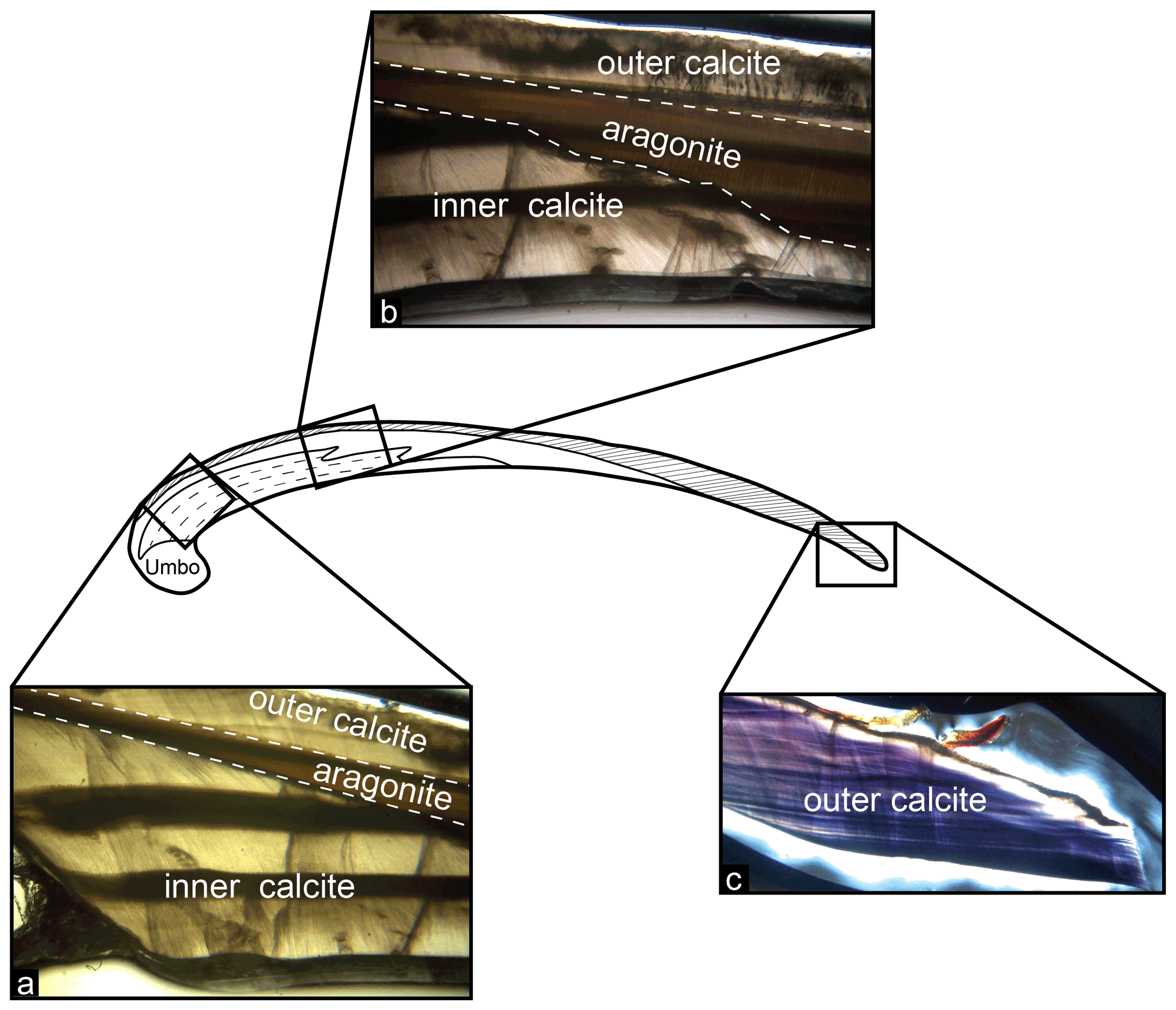
Figure 3Shell structure and mineralogical layering in M. californianus. (a) Photo taken under light microscope focused at the region of interest showing the three mineralogical layers. Dashed lines indicate boundaries between inner calcite, aragonite, and outer calcite layers. (b) Photo taken towards the middle of the cross section showing that the inner calcite layer tapers to an end. (c) Photo taken at the posterior margin of the cross section at the commissure, where the outer calcite layer is the only layer present.
In thin section, the aragonite layer was visually distinct from the fan- and blade-like prisms characteristic of biogenic calcite. Faint banding did appear in portions of the aragonite layer; in some specimens, the banding appeared continuous with the dark–light banding in the inner calcite layer (Fig. 3b). The nacreous aragonite layer began at or near the umbo toward the outer margin of the shell but did not extend all the way to the commissure in any specimen. Under plane-polarized light, the aragonite layer appeared brown in color and contained tabular crystals oriented parallel to the shell's surface. The innermost layer of prismatic calcite near the anterior margin was microstructurally similar to the outer calcite layer, although the inward growth direction of the inner calcite layer adds to the shell thickness rather than shell length. The inner calcite layer was also the only layer to contain thick, strongly expressed dark–light-band pairs (Fig. 3a). The most recently formed growth band, or terminal band, is the innermost band distal to the outer calcite layer.
Shell morphology is controlled in part by the growth rates of each mineralogical layer, since the inner calcite layer contributes mainly to valve thickness, and the outer calcite layer contributes mainly to shell length. There was a statistically significant positive relationship between the inner calcite layer and shell length (linear regression, R2 = 0.36, p < 0.001, F1,38 = 21.49; inner-calcite thickness (mm) = 0.03 ⋅ shell length (mm) − 0.06).
Thick dark–light growth band pairs were present in the inner calcite layer (Fig. 3a) and faint, indistinguishable bands appeared in the outer calcite layer (Fig. 3c). The inner calcite layer of all specimens contained an average of three growth band pairs, ranging from 0 to 10 pairs per specimen, while the bands in the outer calcite layer were unquantifiable due to their faint and inconsistent expression. Growth band contrast (visual distinction between dark and light banding) and pattern (number of band pairs, color of terminal band, and band thickness) varied widely across specimens (Table S1 in the Supplement). Standardized gray-value variance was used as a proxy for growth band contrast. Mean standardized gray-value variance of all specimens (n= 40) was 0.0 with a standard deviation of 1.0. High standardized gray-value variance is a quantitative indicator of a high contrast between dark and light bands, interpreted as strongly expressed banding. Conversely, low standardized gray-value variance is an indicator of low dark–light-band contrast, interpreted as weakly expressed banding (see Fig. S4 in the Supplement for examples of high- and low-contrast banding).
To determine whether inner-calcite dark–light banding continues to form throughout ontogeny, we used shell length as an indicator of relative ontogenetic age. We applied reduced major axis (RMA) regression to assess the relationship between dark–light-band pairs and shell length (Fig. 4). We found weakly positive and statistically significant correlation between shell length and dark–light-band pairs with greater variance among larger (older) individuals (RMA regression, R2 = 0.39, p < 0.001; number of dark–light pairs = 0.14 ⋅ shell length (mm) − 4.9).
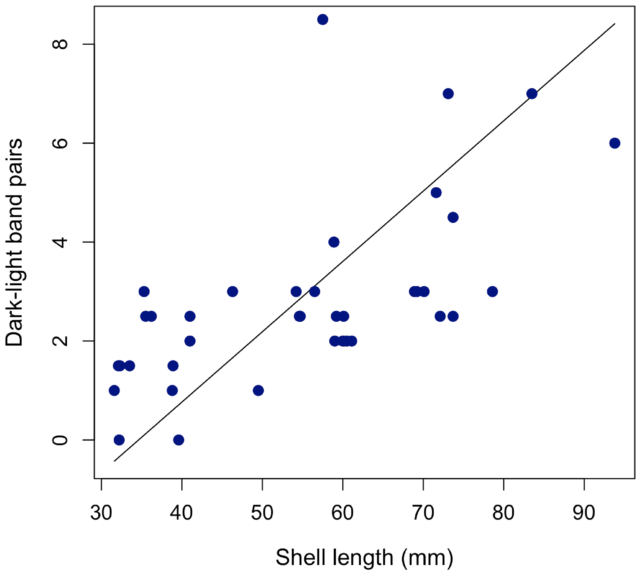
Figure 4Relationship between shell length and number of growth band pairs for all 40 shells with an RMA regression line plotted. Number of dark–light pairs = 0.14 ⋅ shell length (mm) − 4.9.
Across all specimens, there was no statistically significant relationship between standardized gray-value variance (an indicator of growth band contrast) and shell length (Pearson's correlation, p= 0.15). Shell characteristics for all specimens are provided in Table S1.
3.2 Micro-environment and growth band contrast
Standardized gray-value variance varied depending on the micro-environment (i.e., tidal position and habitat) (Fig. 5). Growth band contrast was first compared among specimens collected from a protected cove environment (Horseshoe Cove) and the open-coast sites (BMR and Portuguese Beach) (Fig. 5a). Specimens from open-coast habitats had a lower and broader range of gray-value variance (mean ± σ = 0.37 ± 1.26, n= 17) than cove specimens (mean ± σ = −0.27 ± 0.66, n= 23). Nearly all specimens with high growth band contrast (standardized gray-value variance > 1) were collected from an open-coast habitat, although this relationship was not statistically significant (Welch's two-sample t test, t = −1.91, p= 0.07).
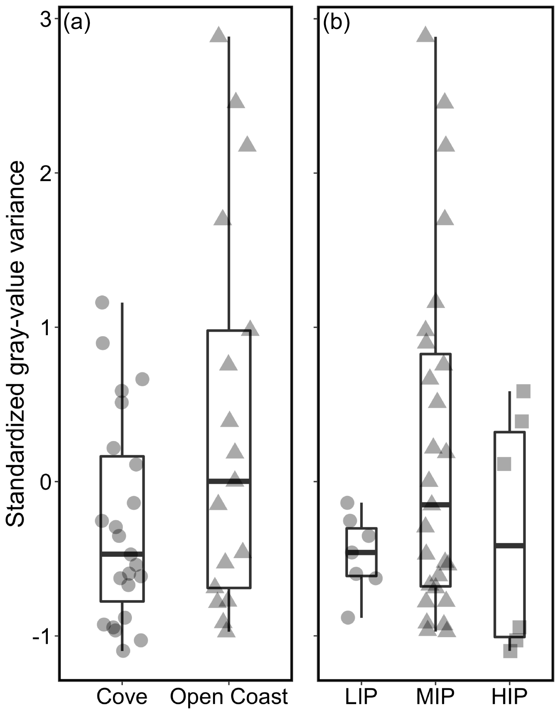
Figure 5Relationships between micro-habitat and standardized gray-value variance as a proxy for growth band contrast. High standardized gray-value variance is indicative of high contrast between dark and light bands. (a) Cove specimens are from Horseshoe Cove at BMR, and open-coast specimens are from an open-coast site within BMR and Portuguese Beach. (b) Relationships between intertidal position (LIP: low intertidal position; MIP: middle intertidal position; HIP: high intertidal position) and standardized gray-value variance for all 40 specimens.
Specimens were also categorized by intertidal position (LIP, MIP, and HIP) (Fig. 5b). All specimens collected from the LIP and HIP had low gray-value variances (ranging from −1.1 to 0.59, n= 13). Specimens with the highest contrast in gray values were collected from the MIP (ranging from −0.97 to 2.88, n= 27). Even when archival shells were excluded (all archival shells were collected from the MIP), the modern shells displayed the same patterns, with the greatest range and highest standardized gray-value variance still found in MIP specimens only (Fig. S5 in the Supplement).
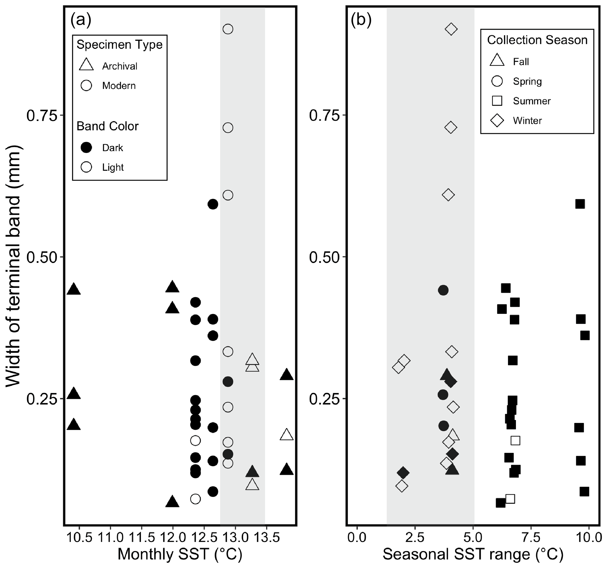
Figure 6Relationships between SST, width of the terminal band, color of the terminal band, specimen type, and collection season for all 40 specimens. Filled (black) points represent dark terminal bands, and open (white) points represent light terminal bands in both plots. (a) Relationships between mean monthly SST during the month of collection, color of the terminal band, and width of the terminal band. Shaded bar represents approximate monthly SST range over which most specimens are associated with light terminal bands (12.75–13.5 ∘C). Specimen type specified with point shapes (see legend a). (b) Relationships between the seasonal SST range (mean daily SST maximum – mean daily SST minimum for each season of collection), color of the terminal band, and width of the terminal band. Shaded bar highlights that most terminal light bands are associated with a seasonal SST range < 5 ∘C. Collection season specified with point shapes (see legend b).
3.3 Oceanographic conditions and growth band pattern
Thirteen specimens precipitated a light terminal band. Out of these 13 specimens, 10 were collected during months with an average monthly SST between 12.75 and 13.5 ∘C (Fig. 6a), and 11 were collected during seasons with a seasonal range in daily SST within 5 ∘C (Fig. 6b). Out of all 40 shells, 27 shells had a dark terminal band, and 24 of these were collected during months with a monthly SST either lower than 12.75 ∘C or higher than 13.5 ∘C. All 6 specimens collected during a month with a monthly average SST ≤ 12 ∘C had a dark terminal band, and 22 out of 24 specimens collected during months cooler than 12.75 ∘C had a dark terminal band (Fig. 6a).
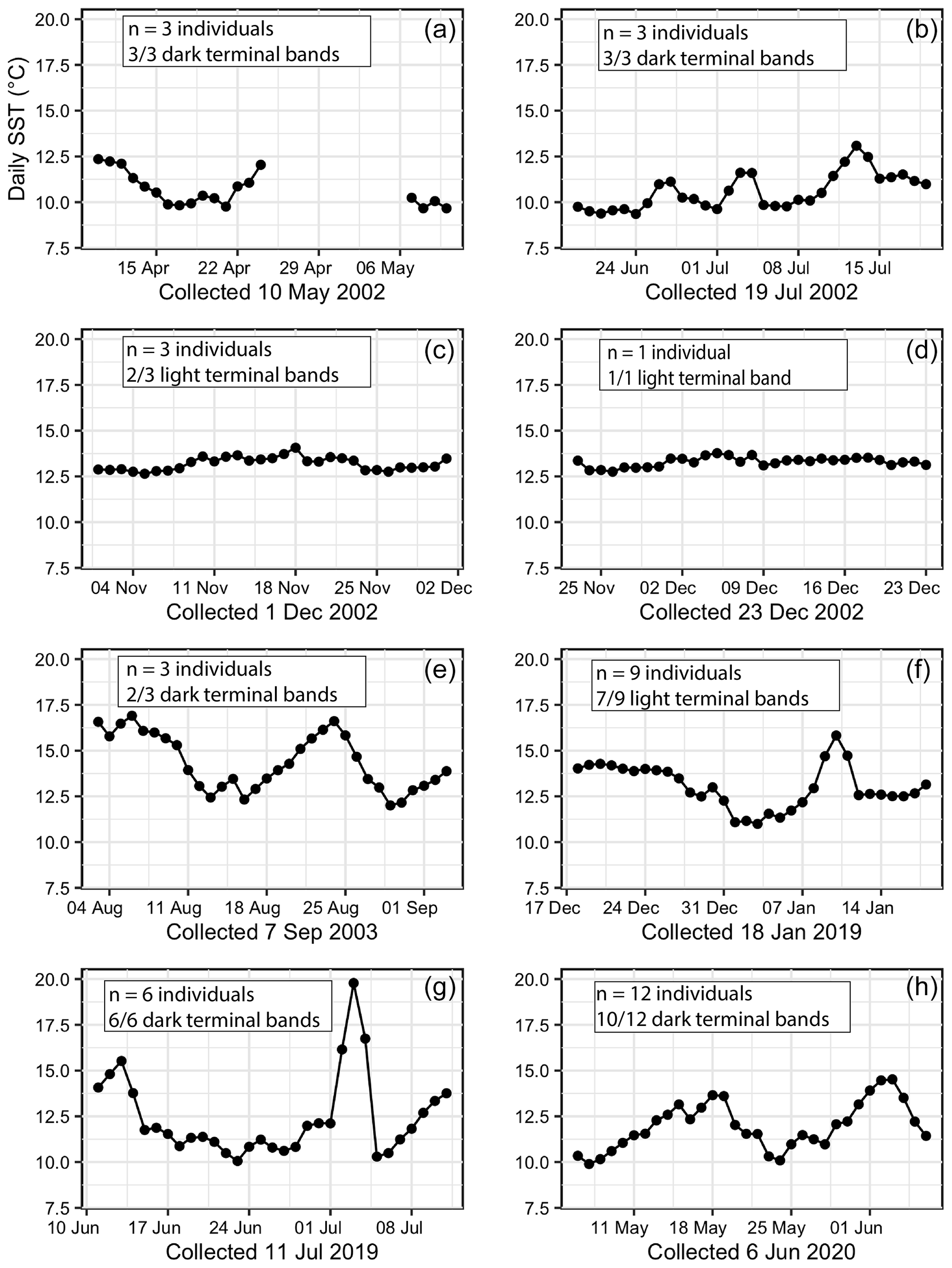
Figure 7Daily temperatures for 30 d prior to the collection date for all 40 specimens. Each plot features the number of specimens collected on that date and the majority terminal-band color. (a) Instrumental error occurred in May 2002. (b) Daily temperatures oscillating between cooler (∼ 9 ∘C) and warmer (∼ 13 ∘C) in July 2002. (c, d) Consistent daily temperatures between 12.25 and 12.5 ∘C in December 2002. (e) Sinusoidal daily temperatures oscillating between ∼ 12 and 17.5 ∘C in September 2003. (f) Daily temperatures prior to the 18 January 2019 collection date were consistent for 2 weeks before slight cooling and 3 d of warming. (g) Highly variable daily temperatures and a 3 d extreme warm spike in July 2019. (h) Daily temperatures oscillating between cooler (∼ 10 ∘C) and warmer (∼ 15 ∘C) in June 2020.
In addition to monthly and seasonal SST patterns, daily SST for the final 30 d of each individual's life were plotted (Fig. 7). Collection dates in December 2002 were preceded by extremely steady daily temperatures between 12.5 and 13 ∘C (n= 4 mussels, and 3 of these specimens had a light terminal band) (Fig. 7c and d). Oscillating warm–cool daily temperatures occurred in July 2002, September 2003, and June 2020 and were closely associated with dark terminal bands (Fig. 7b, e, and h). An extreme warm spike to 20 ∘C occurred over the course of a 3 d long heat wave in July 2019 (Fig. 7g), and all six specimens collected following this event had a dark terminal band. Instrumental error occurred in May 2002, so it was not possible to connect the three specimens with dark terminal bands collected during that month with daily temperature trends (Fig. 7a). Seven out of nine specimens collected in January 2019 had a light terminal band despite a 3 d long temperature spike from 12.5 up to ∼ 16.25 ∘C (Fig. 7f).
The color and width of the terminal band were also assessed in relation to upwelling conditions expressed as BEUTI and CUTI. Of the 13 shells with light terminal bands, 10 appeared in shells collected during months with negative BEUTI and CUTI values. Out of the 27 shells with a dark terminal band, 24 were collected during months where CUTI values were 0.5 or greater and BEUTI values were greater than 5.0. Patterns were similar for both BEUTI and CUTI (Fig. S6 in the Supplement) and strongly covaried with monthly SST (i.e., intense upwelling produces cool conditions, while relaxed upwelling produces warm conditions).
3.4 Temporal trends of shell growth features
On a sub-annual scale, dark–light-band pairs in the inner calcite layer displayed a strong relationship with season of collection in both modern shells (n= 27, collected in 2019 and 2020) and archival shells (n= 13, collected in 2002 and 2003). Of the 21 mussels collected in summer months with increasing temperatures, 19 had a dark band that precipitated as the terminal band (90.5 %). Of the 13 mussels collected in winter months with stable temperatures, 10 had a light band that precipitated last (76.9 %). Only six mussels were collected during spring and fall (n= 3 each), but all of the shells collected in the spring have a dark band that precipitated as the terminal band, and two out of the three shells collected in fall have a dark band that precipitated as the terminal band (Table S1). We identified a statistically significant relationship between the season of collection and color of the terminal band (chi-square test, χ2 = 18.193; df = 3, p= 0.0004).

Figure 8Box plot showing the range of standardized ratio of inner-calcite thickness to shell length in archival and modern specimens. White diamond denotes mean.
Decade-specific growth trends were assessed by comparing shell characteristics between archival and modern shells. We compared gray-value variance measurements, ratios of the inner-calcite-layer thickness to valve length, and the percent of light bands per shell (Fig. 8). The standardized gray-value variance was significantly lower in modern shells than in the archival shells (Welch's two-sample t test, t=2.27; df = 14.68; p= 0.039; Fig. 8a). The standardized ratios of the inner-calcite thickness relative to the shell length were significantly lower in modern shells than they were in shells collected in 2002 and 2003 (Kruskal–Wallis rank sum test, p < 0.05) (Fig. 8b).
There was no statistical difference between the percent of light bands in archival versus modern shells (Welch's two-sample t test, p= 0.5) (Fig. S7 in the Supplement). The percent of light bands ranged from 0.15 to 0.61 in all specimens, with a mean of 0.43 and a median of 0.46.
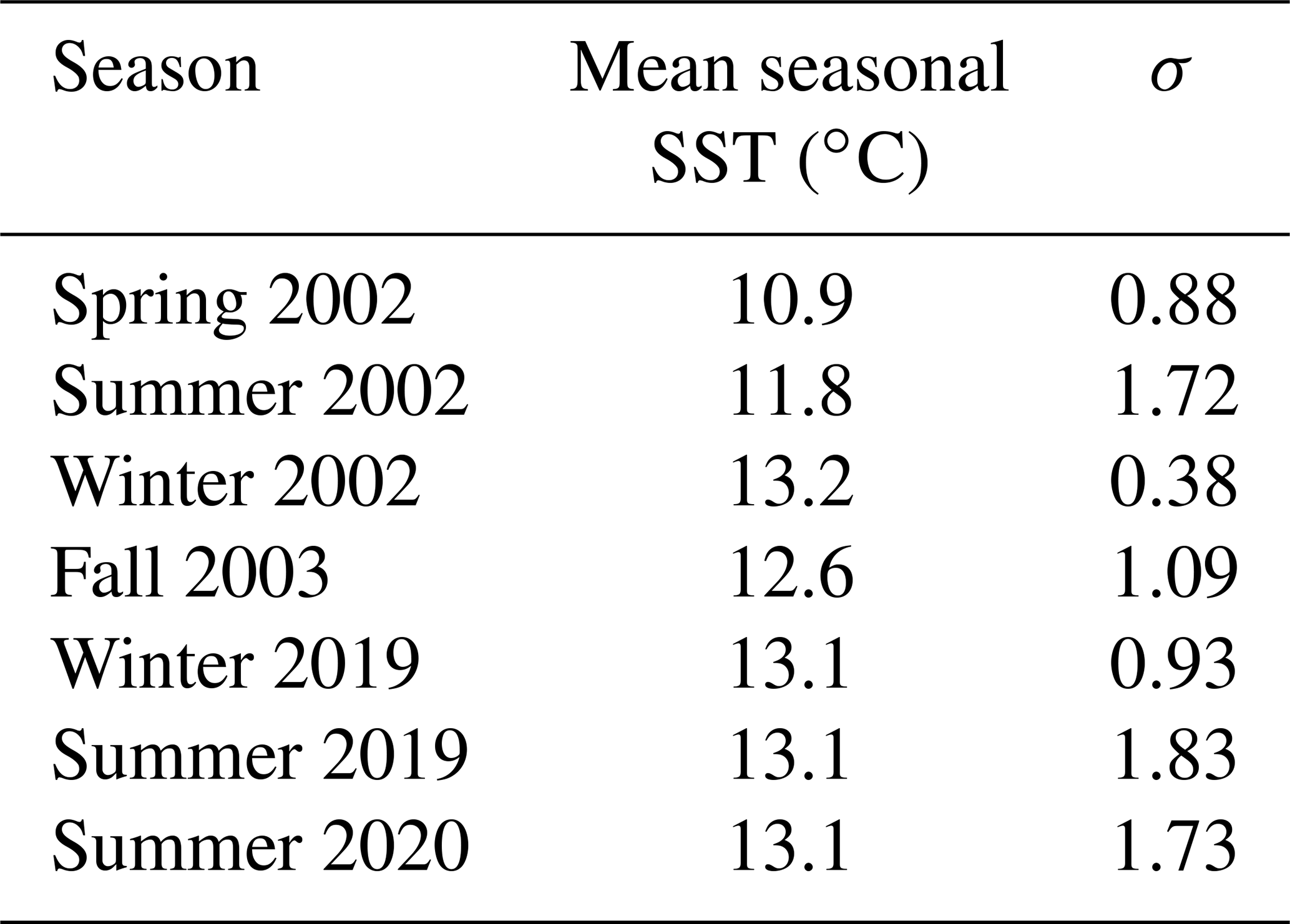
Table 2Seasonally averaged SST (∘C) for the specific collection season of each mussel (n= 40 over eight collection dates across seven different seasons) and standard deviation for each calendar season of the study period. Spring: March through May; summer: June through August; fall: September through November; winter: November through January.
3.5 Evaluation of oceanographic data
Using BOON SST data for Bodega Bay and monthly upwelling indices at 38∘ N from BEUTI and CUTI, we assessed daily, monthly, seasonal, and annual conditions for the study periods 1995–2004 and 2011–2020 to provide environmental context for the archival and modern shells, respectively. Over both study periods, the lowest SSTs occurred in April through June, and the warmest months of the year were August through November (Fig. S3). Temperatures changed drastically from April through July, with SST shifting from one annual extreme (<10 ∘C) to another (∼ 16 ∘C) within a 3-month period (Fig. S1). The coolest season of both study periods was spring of 2002, while the warmest season was winter of 2002 (Table 2). Summers recorded higher daily temperature variability (σ > 1.5) than winter and spring months (σ < 1).
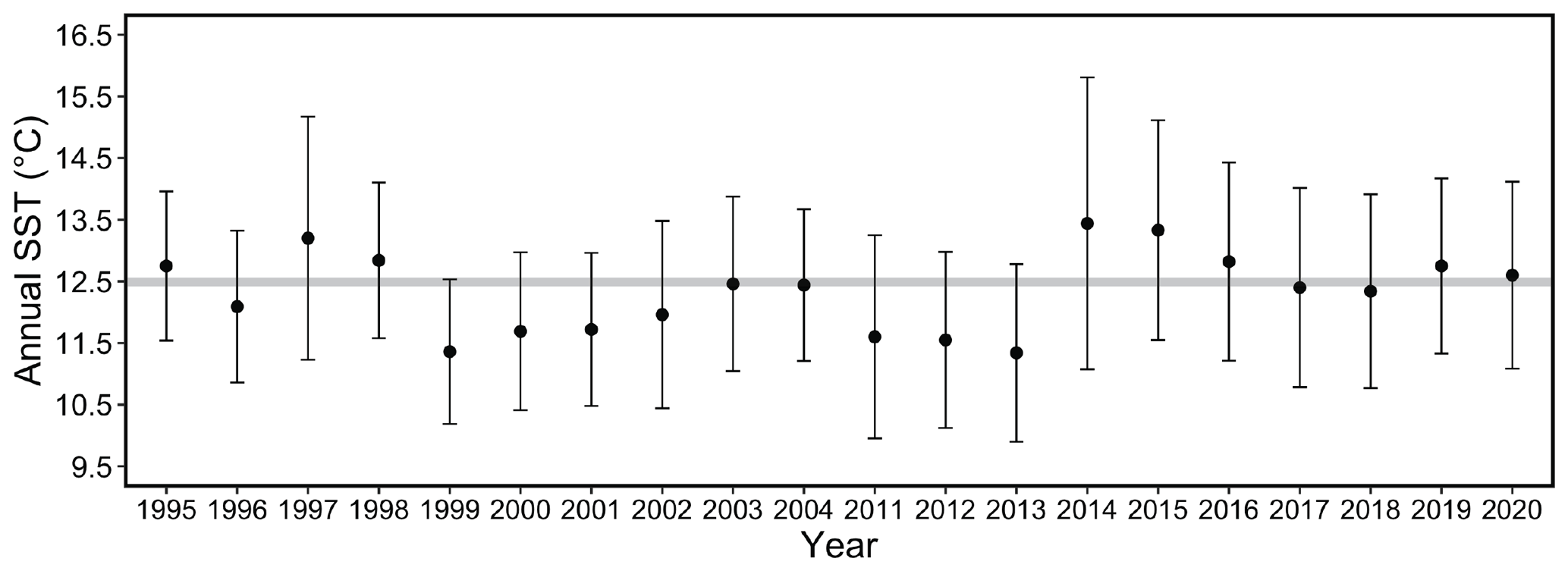
Figure 9Mean annual SST for each year of the study period. Error bars represent the standard deviation of daily temperatures over the course of each year. Shaded bar plotted at 12.5 ∘C for ease of visual comparison across annual means from 1995 to 2004 and 2011 to 2020.
Comparing the two study periods revealed no significant difference in mean monthly or annual SST values between the 1995–2004 period and 2011–2020 period (two-sample t test, p= 0.12 and 0.58, respectively). However, greater variance in SST occurred in the more recent study period (F test, F=0.6499; dfnum = 3140, dfdenom = 3630; p < 0.001). The mean annual SST was at or below 12.5 ∘C from 1999 to 2004 and near or above 12.5 ∘C from 2014 to 2020 (Fig. 9).
Both the archival and modern upwelling indices recorded weak upwelling during winter with low productivity (Fig. S8 in the Supplement). Spring and early summer (March through June) is characterized by strong upwelling and high productivity, reflected by high BEUTI and CUTI values. Comparisons between upwelling indices revealed a significant difference in mean monthly CUTI values (two-sample t test, t = −3.3339; df = 7669; p= 0.0008) and variance values (F test, F = 1.1503; dfnum = 4017, dfdenom = 3652; p < 0.001) with higher averages and greater variance occurring in the more recent study period (Fig. S2). The same shift was present in the BEUTI record for both average values (two sample t test, t = −5.5299; df = 7669; p < 0.001) and variance (F test, F = 0.902; dfnum = 4017, dfdenom = 3652; p= 0.001), with significantly higher means and greater variance of BEUTI values in 2011–2020 than in 1995–2004.
4.1 Interpreting mineralogical layering and growth bands
Visual inspection under a reflected-light microscope showed three distinguishable mineralogical layers in Bodega Bay specimens (Fig. 3), regardless of collection location or shell length. The mineralogical layering of M. californianus was first described based on visual inspection and X-ray diffraction (XRD) analysis 6 decades ago (Dodd, 1963, 1964) and had not been re-examined in the literature prior to this study, leading to inconsistencies in the M. californianus literature. While all Mytilus congeners precipitate both calcite and aragonite in two distinct layers in their shell (Taylor et al., 1969), M. californianus is the only Mytilus species known to precipitate a secondary layer of calcite. A few previous M. californianus studies (e.g., McCoy et al., 2011, 2018; Pfister et al., 2011, 2016) noted the presence of a secondary inner layer of calcite, as initially described by Dodd (1964) and corroborated by the specimens analyzed here, but M. californianus shell mineralogy is often described or assumed to be bi-layered, with an outer calcite layer and an inner aragonite layer only.
The dark–light bands within the inner calcite layer of M. californianus have a different appearance from growth lines in many other well-studied bivalve species. Growth bands in M. californianus are thick bands alternating between dark and light increments, rather than thin lines that demarcate periods of accretionary growth. For example, in Arctica islandica and Saxidomus gigantea, thin growth lines result from growth cessation and reliably represent growth shutdown during winter, while light increments represent shell growth over the rest of the year (Schöne et al., 2005a; Hallmann et al., 2009; Burchell et al., 2013). Growth lines are understood to represent points at which calcification ceased and subsequently resumed, but the formation of dark–light banding is more complex. The dark–light bands in M. californianus are more comparable to those found in Crassostrea virginica, which are described as alternating dark and light increments visible in the cross section (Kirby et al., 1998; Andrus and Crowe, 2000; Surge et al., 2001; Zimmt et al., 2019; Table 1). Dark–light bands could represent alternating periods of shell deposition during aerobic and anaerobic respiration, with light bands forming during aerobiosis and dark bands forming during anaerobiosis (Lutz and Rhoads, 1977; Gordon and Carriker, 1978; McCoy et al., 2011). Under optimal conditions, such as during immersion or moderate-to-warm temperatures, M. californianus gapes and respires aerobically, and during sub-optimal conditions, such as during aerial exposure and/or extreme temperatures, M. californianus closes its valves and respires anaerobically (Bayne et al., 1976; Connor and Gracey, 2011; Connor et al., 2016). During anaerobiosis, glucose and aspartate ferment, resulting in the production of alanine and succinate, which is then converted to propionate if anaerobic conditions persist for several days (Connor and Gracey, 2011). Succinate is an acidic end product of anaerobiosis, which may contribute to the production of an organic-rich dark band in the shell's inner calcite layer (McCoy et al., 2011). While it has been suggested that M. californianus partially dissolves its own shell during anaerobiosis in order to neutralize the acidic end products of its own metabolism (Gordon and Carriker, 1978; McCoy et al., 2011), other sclerochronological studies have dismissed the anaerobiosis–dissolution theory to argue instead that the growth band pattern in bivalve mollusks is the visual result of fluctuating calcification rates and changes in crystallographic size and orientation (Schöne and Surge, 2012). While the mechanism that produces dark bands in M. californianus has not been identified, dark bands could be (1) dissolution bands, (2) organic-rich bands, (3) the visual expression of slow calcite biomineralization during sub-optimal growing conditions, or (4) a combination of multiple processes. Further investigation of the relationships (if any) among anaerobiosis, dissolution, and growth features in intertidal bivalves like M. californianus would help elucidate the mechanism of growth band formation in greater detail.
Because the physiological process behind dark-band formation is unknown, it remains unclear if one pair of dark–light bands reliably represents 1 year in Bodega Bay specimens, as has been documented in populations of M. californianus from Tatoosh Island and Seattle, Washington (McCoy et al., 2011, 2018; Pfister et al., 2011, 2016). If dark bands in the inner calcite layer were to form annually in response to temperature cycles, then individuals of the same size class (and therefore age cohort) should have the same number of dark–light-band pairs. Shell growth rate monitoring of M. californianus individuals from Bodega Bay and other northern California coastal sites has shown that individual shells < 80 mm long can grow between 0 and 1 mm per month (Smith et al., 2009). A young individual with an initial size of 10 mm growing 1 mm per month would grow ∼ 30 mm in 30 months, or 2.5 years. This individual would be 40 mm long with 2.5 dark–light pairs after 2.5 years. While multiple specimens analyzed here did follow these estimates (Fig. 4), many individuals contain far fewer dark–light-band pairs than their shell length would indicate, so it would not be possible to visually cross-date, as can be done in other bivalve species (e.g., Panopea abrupta) (Black et al., 2008).
The statistically significant positive correlation between shell length (a relative proxy for ontogenetic age) and dark–light-band pairs within the inner calcite layer (RMA regression, R2=0.39, p < 0.001; Fig. 4) suggests that M. californianus shells continue to form dark–light bands in the inner calcite layer as the shell grows posteriorly (i.e., the inner calcite layer thickens as the outer calcite layer lengthens throughout ontogeny). However, constraining calcification rates for M. californianus from northern California is complicated by slow shell growth rates (Smith et al., 2009) and the lack of a reliable ontogenetic age estimate based on shell length. Previous shell growth studies have focused on the fast-growing southern California M. californianus populations (Blanchette et al., 2007; Smith et al., 2009; Ford et al., 2010; Connor and Robles, 2015). An early study conducted 8 decades ago used 1000 mussels growing in La Jolla, California, to estimate that an average M. californianus shell is ∼ 80 mm long after 1 year (Coe and Fox, 1944). However, the latitudinal gradient and local oceanographic differences are strong indicators that the shell-length-based age estimate for southern California mussels is not applicable to northern California mussels, where seawater is significantly cooler and upwelling is more intense. In addition to geographic and oceanographic differences, environmental changes that have occurred in the ∼ 80 years since the study necessitate an updated and site-specific estimate of M. californianus shell growth rate. Extremely low shell ventral-margin extension rates have been reported for M. californianus at Bodega Bay (∼ 0 mm per month) (Smith et al., 2009) and the coast of Washington (∼ 1 mm per month) (Paine, 1976). We found further evidence for markedly lower growth rates for northern M. californianus shells as a result of our collection methodology (Text S1 in the Supplement). The disparity between shell growth rates for northern and southern California mussel populations also influences the age at sexual maturity (Suchanek, 1981). Individuals from southern California reach sexual maturity at ∼ 15–25 mm long, or approximately 4 months after settlement (Coe and Fox, 1944; Jones and Richman, 1995), but the shell length and age at sexual maturity are unknown and certainly different for slower growing northern California mussel shells.
4.2 Relationships between the environment and growth band patterns
We observed relationships between the micro-environment and growth band contrast, with open-coast and MIP specimens containing more strongly expressed dark–light bands than specimens collected from cove or extreme (LIP or HIP) tidal environments (Fig. 5). High standardized gray-value variance was again found only in MIP specimens even when all archival shells were excluded from analysis (since all archival shells are from the MIP at Portuguese Beach; Fig. S5). The similarity in gray-value variance patterns across all sets of MIP specimens indicates that growth band contrast is more strongly controlled by subtle differences in the micro-environment (e.g., aerial immersion time) than by the alongshore coastal oceanographic gradient of the Sonoma Coast. Such differences emphasize the importance of small-scale, within-site variation of calcification patterns for M. californianus, as previously presented by Thakar et al. (2017) and Connor and Robles (2015), for regions like the Sonoma Coast with locally uniform oceanographic patterns. However, in regions with high alongshore variability or locally asynchronous warm/cool periods, differences in local oceanography would also play an important role in influencing calcification patterns. For example, there are significant differences in M. californianus shell growth rates just north and south of Point Conception in southern California, where SSTs and wave exposure vary strongly despite geographic proximity (Blanchette et al., 2007).
In addition to micro-environmental variation, we found relationships between broader oceanographic conditions and shell growth features. Shells collected during months with strong upwelling and high productivity were more likely to have a dark band that precipitated most recently (Fig. S6), indicating that strong upwelling and resultant high food availability does not necessarily cause faster shell growth in M. californianus from northern California. Low temperatures induced by upwelling may outweigh the effects of high food availability on the calcification rate. Temperature – rather than upwelling and food availability – has been previously identified as the primary factor of shell growth rate for M. californianus populations in southern California in field studies (Phillips, 2005; Blanchette et al., 2007). We contribute an additional line of evidence for SST as the strongest control over growth rate in both archival and modern northern M. californianus shells, and we suggest that SST stability (or variability) has a stronger influence on growth band coloration and growth rate than absolute temperature (Fig. 6). While previous studies have suggested that food availability is not a strong driver of calcification for M. californianus because of the lack of relationship between chlorophyll a and shell growth (Phillips, 2005; Blanchette et al., 2007), it is also possible that upwelling-associated low pH can expose mussels to more acidic conditions in their habitats (Feely et al., 2008; Rose et al., 2020). Periods with heavy upwelling in the CCS could hinder calcification or even alter the proportion of shell calcite to aragonite in response to changes in the calcium carbonate saturation state (Bullard et al., 2021). While the heavy upwelling in the CCS offers a natural laboratory for examining low-pH conditions, it may become increasingly difficult to disentangle the impacts of anthropogenic ocean acidification and upwelling-induced low pH on M. californianus, given that wind-driven upwelling has increased along the coast of California in recent decades due to intensifying onshore–offshore atmospheric pressure gradients associated with rising temperatures (García-Reyes and Largier, 2010). Evidence of decadal-scale intensification of upwelling appeared here in the CUTI and BEUTI records.
4.3 Interpreting temporal trends of growth features
Using the season of collection for each shell, we identified a significant relationship between the season and terminal-band color and specifically between winter and light bands (Fig. 6b). While winter is typically the time of year that bivalves in the Northern Hemisphere experience growth slowdown and produce a dark line (Killam and Clapham, 2018, and references therein), our findings from M. californianus support the hypothesis that mussels grow their shell optimally during warmer periods (up to a point) given that December at Bodega Bay has higher mean monthly SSTs and more stable daily SSTs than March through June, making winter months generally warmer than spring months and much less variable than summer months (Table 2; Fig. 6b). We interpret the light band found in the majority of winter-collected shells as an indicator of fast (calcium-carbonate-rich) growth (Schöne and Surge, 2012) occurring during optimal growth conditions for northern California mussel populations when SST is moderate and stable. Dark (slow-growth) bands were closely associated with spring–early summer or during cooler or highly variable periods (Figs. 6 and 7). Dark bands were also found in all specimens that experienced an extreme 3 d long heat wave (20 ∘C) that occurred a week prior to their collection (Fig. 7g), indicating that the M. californianus growth rate slows during variable, cold, or extremely high SSTs. Despite the strong correlation between season and band color, dark–light bands cannot necessarily be used as an indicator of lifespan because the dynamic oceanographic regime at Bodega Bay could result in multiple growth slowdowns within the span of one annual cycle. However, dark bands could potentially be used to reconstruct extreme or variable conditions, while light bands could serve as indicators of stable and moderate periods.
In addition to seasonal variability at Bodega Bay, the intertidal zone experiences extreme environmental variation (temperature and submergence time) on daily and biweekly scales. While tidal cycling does not contribute to the number of dark–light bands in the inner calcite layer (i.e., mussels experience hundreds to thousands of high–low tidal cycles but contain only three dark–light-band pairs on average), tidal variability could play a role in growth band contrast, since the intertidal position (LIP, MIP, and HIP) and standardized gray-value variance were related (Fig. 5). LIP and HIP specimens experience tidal extremes for the longest periods of time (immersion and exposure, respectively) and have low-contrast growth bands. MIP specimens have a wide range of standardized gray-value variance, but all specimens with strongly expressed bands were collected from the MIP only, perhaps because they experienced tidal extremes for shorter periods of time than LIP and HIP specimens.
We calculated the percentage of light bands across all specimens to compare the time spent growing normally (light bands) versus abnormally (dark bands). The average percent of light bands across all specimens was 43 %, and no specimen had a light-band percentage greater than 61 % (Fig. S7). If dark bands precipitate more slowly than light bands yet represent half or more than half of the inner calcite layer of all specimens, then Bodega Bay specimens spend more of their lives experiencing hindered growth rather than normal growth. Interestingly, northern California mussel populations seem to grow their shell during faster “growing windows” when conditions are moderate to warm and stable, but they calcify slowly for a longer period of the year and spend most of their lives experiencing slow-growth conditions. While most light bands are associated with winter (December and January), it is possible that the warmest time of year at Bodega Bay (August through October) could also be part of the growing window for northern California populations of M. californianus, but we did not have enough shells collected in fall months available (n= 3) to confirm this. Out of the three fall-collected shells, one specimen did have a light band that precipitated most recently, which does suggest that fast growth and light-band precipitation can occur during the warm fall months or during any period of the year with sustained conditions that match the optimal range for shell growth. At Bodega Bay, sustained optimal growth conditions are less likely to occur during spring and early summer because of cold and highly variable SST conditions controlled by the seasonal upwelling regime.
We also observed a statistically significant decline in the ratios of inner-calcite thickness to shell length from the archival to the modern specimens, indicating that mussel shells growing in the same location nearly 2 decades apart are thinner relative to their length (Fig. 8b). Both the cross-sectional valve thickness and the thickness of the inner calcite layer have declined overall relative to shell length. The valve thinning could indicate a slowed rate of calcification, that the inner calcite layer now grows for a shorter period of time in the life of the animal, or even that the length of life is declining in modern specimens. Evidence for rapid and recent shell thinning has also been found in Washington M. californianus populations, where cross-sectional shell thickness in modern mussels is significantly thinner than both archival (collected in the 1960s–1970s) and archeological mussel shells (∼ 2420–1000 cal BP) (Pfister et al., 2016). In addition to shell thinning, we found that growth bands in modern shells had significantly lower dark–light-band contrast than the archival shells (Fig. 8a). This provides a new line of evidence for recent changes in shell microstructure occurring in the past 15 years, in addition to previous evidence of increased crystallographic disorder in modern M. californianus shells relative to archival and archeological shells from Washington (McCoy et al., 2018) and a reduction in aragonite deposition relative to calcite in recent M. californianus shells from southern California (Bullard et al., 2021). Due to limitations in the length and availability of oceanographic datasets, we did not aim to link changes in shell growth and the dark–light-band pattern to anthropogenic ocean acidification or lower pH in response to increased CCS upwelling, although SSTs were higher and more variable, and upwelling was significantly stronger in 2011–2020 than in 1995–2004. We suggest that the weakened growth band expression and decline in inner-calcite thickness ratios in the modern shells could be responses to warmer-than-average conditions and/or low-pH conditions associated with stronger upwelling, which can be further explored by applying well-developed geochemical proxies to reconstruct conditions recorded by mussel shells (e.g., δ18O[shell] − SST). However, the primary challenge with sampling the inner calcite layer for stable isotope analysis is the fine-resolution sampling required; the inner calcite layer is ∼ 2 mm thick (mean of n= 40), and individual bands can be extremely thin (on the order of micrometers).
4.4 Potential factors contributing to variability of shell growth features
Given that temperature and upwelling conditions are nested within temporal trends (interannual variability and periodic oceanographic phases), we expected and found significant differences in shell growth patterns between the archival and the modern shells. We observed a high degree of variability in growth band pattern and ratios of the inner-calcite thickness to shell length in both modern and archival specimen categories (Fig. 8). Even when standardized, the variance of the ratio of the inner-calcite thickness to shell length across all specimens was high (σ2 = 7.77), indicating that there is a range of growth rates and dark–light-band formation rates even among specimens experiencing the same or highly similar environmental conditions along the Sonoma Coast. While the three collection sites experience synchronous warm or cool periods, it is possible that small-scale oceanographic variability results in different shell growth patterns at the BMR versus Portuguese Beach open-coast collection sites. However, we found evidence to suggest that relative (rather than absolute) temperature variability is a stronger influence over shell growth patterns (Figs. 6 and 7). Another possible source of variability is the uneven sampling distributions due to the archival specimens available and restrictions on modern sample collection during the COVID-19 pandemic. Regardless of sample size, a certain degree of growth pattern variability is expected depending on the plasticity among individual organisms and on the micro-environment within and across populations. If dark–light banding is mediated by a physiological response to environmental conditions (e.g., a metabolism that alternates between anaerobic and aerobic respiration depending on SST), there can be varying physiological responses among individuals due to micro-environmental gradients in SST or immersion time in the highly variable intertidal zone (Connor and Robles, 2015; Thakar et al., 2017). For food availability, tidal position is a minor factor, since functional-submergence time (the time required for an individual to gape its valves and effectively filter-feed) is uniform across intertidal positions (LIP, MIP, and HIP) for M. californianus (Connor et al., 2016). While low tide and low temperatures have been suggested as conditions that trigger a switch to anaerobic respiration in M. californianus (Connor and Gracey, 2011; McCoy et al., 2011), the temperature threshold for anaerobiosis is unknown and is likely to differ depending on the population's latitude and local oceanographic parameters. For example, northern California mussel populations experience cooler conditions and a narrower range of temperatures (∼ 10–13.5 ∘C mean monthly SST) than southern California mussels, which have been observed to grow most rapidly between 15 and 19 ∘C (Smith et al., 2009). Temperatures approaching 19 ∘C could be outside the range of tolerance for populations from northern California given that SSTs rarely exceed 19 ∘C at Bodega Bay; the BOON SST record documents only 3 d warmer than 19 ∘C over both decade-long study periods. The north–south SST gradient in California may result in slow growth and more frequent dark-band formation for northern mussel populations and optimal growth and light-band formation – and perhaps a greater overall percentage of light bands – for warm-water acclimated southern California mussel populations. A latitudinal gradient in shell growth rate, and therefore growth band pattern, controlled by the CCS' variable upwelling regime is explained by the high plasticity in physiological responses to oceanographic conditions in M. californianus (Dahlhoff and Menge, 1996).
We identified three mineralogical layers in M. californianus: an outer calcite layer with faint indistinguishable banding; a thin nacreous aragonite middle layer; and an inner calcite layer that grows inward, precipitating dark–light-band pairs. The improved understanding of shell layering and growth directionality has important implications for paleoceanography and archeology, which require geochemical subsampling approaches and proxy equations tailored to growth direction and the specific calcium carbonate polymorph. Within the genus Mytilus, the inner calcite layer is unique to M. californianus and may be a useful layer for the reconstruction of extreme conditions and determination of the season of collection due to strongly expressed growth banding, although the contrast between dark–light bands is variable and dependent on tidal position and habitat type.
We documented a strongly positive and statistically significant correlation among light bands and winter collection months, moderate SST (average monthly SST between 12.75 and 13.5 ∘C and average seasonal temperature of ∼ 12 ∘C), and weak upwelling (CUTI and BEUTI < 0) at Bodega Bay, indicating that light bands are more likely to precipitate during growing windows with relatively constant SSTs. Slower or halted growth, recorded as dark bands, is more likely to occur during spring through early summer, or when conditions are highly variable or locally extreme, although it is uncertain which conditions are considered “extreme” for intertidal M. californianus populations in northern California. We also found that low temperatures may result in slow shell growth and dark-band formation even during periods of upwelling-induced productivity. Interestingly, most specimens analyzed here contained a greater percentage of dark bands than light bands, suggesting that the growth slowdown period is longer than the growing window for Bodega Bay mussels and that mussels spend more of the year – and more of their lives – experiencing hindered growth rather than normal growth.
A shift in calcification patterns from archival (2002–2003) to modern (2019–2020) mussels is also documented here. The statistically significant decline in growth band contrast and the ratios of inner-calcite thickness to shell length indicate that M. californianus is growing more slowly or calcifying less in 2019–2020 than this species was less than 2 decades ago at the same location. The spatial and temporal variability of M. californianus shell growth from Bodega Bay highlights the need for future site-specific calibration of growth band patterns and comparisons through time. Given that M. californianus is an ecologically important foundation species and its shell appears to respond to and sensitively record environmental changes, analysis of the relationships among shell growth features, environmental conditions (SST, pH, and upwelling), and community ecology should be investigated to assess whether these shifts in calcification patterns will have negative impacts for M. californianus and the biologically rich intertidal community that this species supports.
All shell data collected for this paper are available in the Supplement. BOON data are available online at https://boon.ucdavis.edu/ (Bodega Ocean Observing Node, 2020), and all upwelling (CUTI and BEUTI) data are available online at https://oceanview.pfeg.noaa.gov/products/upwelling/dnld (NOAA Fisheries, 2018) and https://mjacox.com/upwelling-indices/ (Jacox et al., 2018b).
The supplement related to this article is available online at: https://doi.org/10.5194/bg-19-329-2022-supplement.
VPV, SJC, and TMH conceptualized and designed the project. VPV completed data collection and wrote the manuscript. All authors contributed to data analysis and the editing of the paper.
The contact author has declared that neither they nor their co-authors have any competing interests.
Publisher's note: Copernicus Publications remains neutral with regard to jurisdictional claims in published maps and institutional affiliations.
This material is based upon work supported by the National Science Graduate Research Fellowship (grant no. 2036201). We thank Jackie Sones for access and assistance at the Bodega Marine Reserve and Zachary Oretsky for assisting with mussel collection. We thank Ann Russell for providing access to archival mussel shells. All thin sections were prepared by Greg Baxter. Leslie Garcia helped to calibrate scales for thin-section images. John Largier provided helpful input about Sonoma Coast oceanography. Thoughtful reviews by Daniel Killam and Alan Wanamaker Jr. improved this paper.
This research was supported by the Geological Society of America (to Veronica Padilla Vriesman), the Cordell Durrell Field Geology Fund (to Veronica Padilla Vriesman), the Mildred E. Mathias Graduate Student Research Grant (to Veronica Padilla Vriesman), and the National Science Foundation (nos. OCE 1832812 to Tessa M. Hill and 2036201 to Veronica Padilla Vriesman).
This paper was edited by Ny Riavo G. Voarintsoa and reviewed by Daniel Killam and Alan D. Wanamaker Jr.
Andrus, C. F. T. and Crowe, D. E.: Geochemical analysis of Crassostrea virginica as a method to determine season of capture, J. Archaeol. Sci., 27, 33–42, https://doi.org/10.1006/jasc.1999.0417, 2000.
Bayne, B. L., Bayne, C. J., Carefoot, T. C., and Thompson, R. J.: The physiological ecology of Mytilus californianus Conrad, Oecologia, 22, 211–228, https://doi.org/10.1007/BF00344793, 1976.
Black, B. A. B. A., Gillespie, D. C. G. C., MacLellan, S. E. M. E., and Hand, C. M. H. M.: Establishing highly accurate production-age data using the tree-ring technique of crossdating: a case study for Pacific geoduck (Panopea abrupta), Can. J. Fish. Aquat., 65, 2572–2578, https://doi.org/10.1139/F08-158, 2008.
Blanchette, C. A., Helmuth, B., and Gaines, S. D.: Spatial patterns of growth in the mussel, Mytilus californianus, across a major oceanographic and biogeographic boundary at Point Conception, California, USA, J. Exp. Mar. Bio. Ecol., 340, 126–148, https://doi.org/10.1016/j.jembe.2006.09.022, 2007.
Bodega Ocean Observing Node: Shorestation Seawater Data, BML Seawater Temperature Daily, 1995–2004 and 2011–2020, Bodega Ocean Observing Node [data set], available at: https://boon.ucdavis.edu/data-access/products/seawater/bml_seawater_temperature_daily (last access: November 2021), 2020.
Braje, T. J., Kennett, D. J., Erlandson, J. M., and Culleton, B. J.: Human impacts on nearshore shellfish taxa: a 7,000 year record from Santa Rosa Island, California, Am. Antiquity, 72, 735–756, https://doi.org/10.2307/25470443, 2007.
Braje, T. J., Rick, T. C., Willis, L. M., and Erlandson, J. M.: Shellfish and the Chumash: marine invertebrates and complex hunter-gatherers on late Holocene San Miguel Island, California, N. Am. Archaeol., 32, 267–290, https://doi.org/10.2190/NA.32.3.c, 2011.
Braje, T. J., Rick, T. C., and Erlandson, J. M.: A trans-Holocene historical ecological record of shellfish harvesting on California's Northern Channel Islands, Quaternary Int., 264, 109–120, https://doi.org/10.1016/j.quaint.2011.09.011, 2012.
Bullard, E. M., Torres, I., Ren, T., Graeve, O. A., and Roy, K.: Shell mineralogy of a foundational marine species, Mytilus californianus, over half a century in a changing ocean, P. Natl. Acad. Sci. USA, 118, e2004769118, https://doi.org/10.1073/pnas.2004769118, 2021.
Burchell, M., Cannon, A., Hallmann, N., Schwarcz, H. P., and Schöne, B. R.: Refining estimates for the season of shellfish collection on the Pacific Northwest Coast: applying high-resolution stable oxygen isotope analysis and sclerochronology, Archaeometry, 55, 258–276, https://doi.org/10.1111/j.1475-4754.2012.00684.x, 2013.
Butler, P. G., Wanamaker J. R., A. D., Scourse, J. D., Richardson, C. A., and Reynolds, D. J.: Variability of marine climate on the North Icelandic Shelf in a 1356-year proxy archive based on growth increments in the bivalve Arctica islandica, Palaeogeogr. Palaeocl., 373, 141–151, https://doi.org/10.1016/j.palaeo.2012.01.016, 2013.
Campbell, B. and Braje, T. J.: Estimating California mussel (Mytilus californianus) size from hinge fragments: a methodological application in historical ecology, J. Archaeol. Sci., 58, 167–174, https://doi.org/10.1016/j.jas.2015.02.007, 2015.
Cannon, A. and Burchell, M.: Reconciling oxygen isotope sclerochronology with interpretations of millennia of seasonal shellfish collection on the Pacific Northwest Coast, Quaternary Int., 427, 184–191, https://doi.org/10.1016/j.quaint.2016.02.037, 2017.
Checkley, D. M. and Barth, J. A.: Patterns and processes in the California Current System, Prog. Oceanogr., 83, 49–64, https://doi.org/10.1016/j.pocean.2009.07.028, 2009.
Coe, W. R. and Fox, D. L.: Biology of the California sea-mussel (Mytilus californianus). iii. Environmental conditions and rate of growth, Biol. Bull., 87, 59–72, https://doi.org/10.2307/1538129, 1944.
Connor, K. M. and Gracey, A. Y.: High-resolution analysis of metabolic cycles in the intertidal mussel Mytilus californianus, Am. J. Physiol.-Reg. I, 302, R103–R111, https://doi.org/10.1152/ajpregu.00453.2011, 2011.
Connor, K. M. and Robles, C. D.: Within-site variation of growth rates and terminal sizes in Mytilus californianus along wave exposure and tidal gradients, Biol. Bull., 228, 39–51, https://doi.org/10.1086/BBLv228n1p39, 2015.
Connor, K. M., Sung, A., Garcia, N. S., Gracey, A. Y., and German, D. P.: Modulation of digestive physiology and biochemistry in Mytilus californianus in response to feeding level acclimation and microhabitat, Biol. Open, 5, 1200–1210, https://doi.org/10.1242/bio.019430, 2016.
Dahlhoff, E. and Menge, B.: Influence of phytoplankton concentration and wave exposure on the ecophysiology of Mytilus californianus, Mar. Ecol. Prog. Ser., 144, 97–107, https://doi.org/10.3354/meps144097, 1996.
Dever, E. P. and Lentz, S. J.: Heat and salt balances over the northern California shelf in winter and spring, J. Geophys. Res., 99, 16001–16017, https://doi.org/10.1029/94JC01228, 1994.
Dodd, J. R.: Paleoecological implications of shell mineralogy in two pelecypod species, J. Geol., 71, 1–11, 1963.
Dodd, J. R.: Environmentally controlled variation in the shell structure of a pelecypod species, J. Paleontol., 9, 1065–1071, 1964.
Feely, R. A., Sabine, C. L., Hernandez-Ayon, J. M., Ianson, D., and Hales, B.: Evidence for upwelling of corrosive “acidified” water onto the continental shelf, Science, 320, 1490–1492, https://doi.org/10.1126/science.1155676, 2008.
Ferguson, J. E., Johnson, K. R., Santos, G., Meyer, L., and Tripati, A.: Investigating δ13C and Δ14C within Mytilus californianus shells as proxies of upwelling intensity: δ13C and Δ14C in Mytilus shells, Geochem. Geophy. Geosy., 14, 1856–1865, https://doi.org/10.1002/ggge.20090, 2013.
Ford, H. L., Schellenberg, S. A., Becker, B. J., Deutschman, D. L., Dyck, K. A., and Koch, P. L.: Evaluating the skeletal chemistry of Mytilus californianus as a temperature proxy: Effects of microenvironment and ontogeny, Paleoceanography, 25, PA1203, https://doi.org/10.1029/2008PA001677, 2010.
Freitas, P., Clarke, L. J., Kennedy, H., Richardson, C., and Abrantes, F.: , , and stable-isotope (δ18O and δ13C) ratio profiles from the fan mussel Pinna nobilis: seasonal records and temperature relationships, Geochem. Geophy. Geosy., 6, Q04D14, https://doi.org/10.1029/2004GC000872, 2005.
Freitas, P., Clarke, L. J., Kennedy, H., and Richardson, C.: The potential of combined Mg/Ca and δ18O measurements within the shell of the bivalve Pecten maximus to estimate seawater δ18O composition, Chem. Geol., 291, 286–293, https://doi.org/10.1016/j.chemgeo.2011.10.023, 2012.
García-Reyes, M. and Largier, J.: Observations of increased wind-driven coastal upwelling off central California, J. Geophys. Res., 115, C04011, https://doi.org/10.1029/2009JC005576, 2010.
García-Reyes, M. and Largier, J. L.: Seasonality of coastal upwelling off central and northern California: New insights, including temporal and spatial variability, J. Geophys. Res., 117, C03028, https://doi.org/10.1029/2011JC007629, 2012.
Gillikin, D. P., Dehairs, F., Lorrain, A., Steenmans, D., Baeyens, W., and André, L.: Barium uptake into the shells of the common mussel (Mytilus edulis) and the potential for estuarine paleo-chemistry reconstruction, Geochim. Cosmochim. Acta, 70, 395–407, https://doi.org/10.1016/j.gca.2005.09.015, 2006.
Gordon, J. and Carriker M. R.: Growth lines in a bivalve mollusk: subdaily patterns and dissolution of the shell, Science, 202, 519–521, https://doi.org/10.1126/science.202.4367.519, 1978.
Hallmann, N., Burchell, M., Schöne, B. R., Irvine, G. V., and Maxwell, D.: High-resolution sclerochronological analysis of the bivalve mollusk Saxidomus gigantea from Alaska and British Columbia: techniques for revealing environmental archives and archaeological seasonality, J. Archaeol. Sci., 36, 2353–2364, https://doi.org/10.1016/j.jas.2009.06.018, 2009.
Hallmann, N., Burchell, M., Brewster, N., Martindale, A., and Schöne, B. R.: Holocene climate and seasonality of shell collection at the Dundas Islands Group, northern British Columbia, Canada – A bivalve sclerochronological approach, Palaeogeogr. Palaeocl., 373, 163–172, https://doi.org/10.1016/j.palaeo.2011.12.019, 2013.
Hickey, B. M. and Banas, N. S.: Oceanography of the U.S. Pacific Northwest coastal ocean and estuaries with application to coastal ecology, Estuaries, 26, 1010–1031, https://doi.org/10.1007/BF02803360, 2003.
Huyer, A.: Coastal upwelling in the California Current system, Prog. Oceangr., 12, 259–284, https://doi.org/10.1016/0079-6611(83)90010-1, 1983.
Jacox, M. G., Edwards, C. A., Hazen, E. L., and Bograd, S. J.: Coastal upwelling revisited: Ekman, Bakun, and improved upwelling indices for the U.S. West Coast, J. Geophys. Res.-Oceans, 123, 7332–7350, https://doi.org/10.1029/2018JC014187, 2018a.
Jacox, M. G., Edwards, C. A., Hazen, E. L., and Bograd, S. J.: New Upwelling Indices for the U.S. West Coast, NOAA Fisheries – Southwest Fisheries Science Center [data set], available at: https://mjacox.com/upwelling-indices/ (last access: November 2021), 2018b.
Jazwa, C. S. and Kennett, D. J.: Sea mammal hunting and site seasonality on western San Miguel Island, California, J. Calif. Gt. Basin Anthropol., 36, 271–291, 2016.
Jones, D. S. and Quitmyer, I. R.: Marking time with bivalve shells: oxygen isotopes and season of annual increment formation, Palaios, 11, 340–346, https://doi.org/10.2307/3515244, 1996.
Jones, T. L. and Kennett, D. J.: Late Holocene Sea Temperatures along the Central California Coast, Quaternary Res., 51, 74–82, https://doi.org/10.1006/qres.1998.2000, 1999.
Jones, T. L. and Richman, J. R.: On mussels: Mytilus californianus as a prehistoric resource, N. Am. Archaeol., 16, 33–58, https://doi.org/10.2190/G5TT-YFHP-JE6A-P2TX, 1995.
Katayama, S. and Isshiki, T.: Variation in otolith macrostructure of Japanese flounder (Paralicthys olivaceus): A method to discriminate between wild and released fish, J. Sea Res., 57, 180–186, https://doi.org/10.1016/j.seares.2006.09.006, 2007.
Kennedy, M. A.: An investigation of hunter–gatherer shellfish foraging practices: archaeological and geochemical evidence from Bodega Bay, California, PhD thesis, University of California, Davis, USA, 3171887, 2004.
Kennedy, M. A., Russell, A. D., and Guilderson, T. P.: A radiocarbon chronology of hunter-gatherer occupation from Bodega Bay, California, USA, Radiocarbon, 47, 265–293, https://doi.org/10.1017/S0033822200019779, 2005.
Killam, D., Thomas, R., Al-Najjar, T., and Clapham, M.: Interspecific and intrashell stable isotope variation among the Red Sea giant clams, Geochem. Geophy. Geosy., 21, e2019GC008669, https://doi.org/10.1029/2019GC008669, 2020.
Killam, D. E. and Clapham, M. E.: Identifying the ticks of bivalve shell clocks: seasonal growth in relation to temperature and food supply, Palaios, 33, 228–236, https://doi.org/10.2110/palo.2017.072, 2018.
Killingley, J. S. and Berger, W. H.: Stable isotopes in a mollusk shell: detection of upwelling events, Science, 205, 186–188, https://doi.org/10.1126/science.205.4402.186, 1979.
Kirby, M. X., Soniat, T. M., and Spero, H. J.: Stable isotope sclerochronology of Pleistocene and Recent oyster shells (Crassostrea virginica), Palaios, 13, 560–569, https://doi.org/10.2307/3515347, 1998.
Klein, R. T., Lohmann, K. C., and Thayer, C. W.: Bivalve skeletons record sea-surface temperature and δ18O via and ratios, Geology, 24, 415–418, https://doi.org/10.1130/0091-7613(1996)024<0415:BSRSST>2.3.CO;2, 1996.
Largier, J. L., Magnell, B. A., and Winant, C. D.: Subtidal circulation over the northern California shelf, J. Geophys. Res.-Oceans, 9 8, 18147–18179, https://doi.org/10.1029/93JC01074, 1993.
Lepofsky, D., Smith, N. F., Cardinal, N., Harper, J., Morris, M., Gitla, E. W., Bouchard, R., Kennedy, D. I. D., Salomon, A. K., Puckett, M., and Rowell, K.: ancient shellfish mariculture on the northwest coast of North America, Am. Antiquity, 80, 236–259, https://doi.org/10.7183/0002-7316.80.2.236, 2015.
Lutz, R. A. and Rhoads, D. C.: Anaerobiosis and a theory of growth line formation, Science, 198, 1222–1227, https://doi.org/10.1126/science.198.4323.1222, 1977.
McCoy, S. J., Robinson, L. F., Pfister, C. A., Wootton, J. T., and Shimizu, N.: Exploring as a pH proxy in bivalves: relationships between Mytilus californianus and environmental data from the northeast Pacific, Biogeosciences, 8, 2567–2579, https://doi.org/10.5194/bg-8-2567-2011, 2011.
McCoy, S. J., Kamenos, N. A., Chung, P., Wootton, T. J., and Pfister, C. A.: A mineralogical record of ocean change: decadal and centennial patterns in the California mussel, Glob. Change Biol., 24, 2554–2562, https://doi.org/10.1111/gcb.14013, 2018.
Mellin, C., Mouillot, D., Kulbicki, M., McClanahan, T. R., Vigliola, L., Bradshaw, C. J. A., Brainard, R. E., Chabanet, P., Edgar, G. J., Fordham, D. A., Friedlander, A. M., Parravicini, V., Sequeira, A. M. M., Stuart-Smith, R. D., Wantiez, L., and Caley, M. J.: Humans and seasonal climate variability threaten large-bodied coral reef fish with small ranges, Nature, 7, 10491, https://doi.org/10.1038/ncomms10491, 2016.
NOAA Fisheries – Southwest Fisheries Science Center: Environmental Research Division: New West Coast Upwelling Indices, NOAA Fisheries – Southwest Fisheries Science Center [data set], available at: https://oceanview.pfeg.noaa.gov/products/upwelling/dnld (last access: January 2022), 2018.
Paine, R. T.: Intertidal community structure, Oecologia, 15, 93–120, https://doi.org/10.1007/BF00345739, 1974.
Paine, R. T.: Size-Limited Predation: an observational and experimental approach with the Mytilus–Pisaster interaction, Ecology, 57, 858–873, https://doi.org/10.2307/1941053, 1976.
Pfister, C. A., McCoy, S. J., Wootton, J. T., Martin, P. A., Colman, A. S., and Archer, D.: Rapid environmental change over the past decade revealed by isotopic analysis of the California mussel in the northeast Pacific, PLoS ONE, 6, e25766, https://doi.org/10.1371/journal.pone.0025766, 2011.
Pfister, C. A., Roy, K., Wootton, J. T., McCoy, S. J., Paine, R. T., Suchanek, T. H., and Sanford, E.: Historical baselines and the future of shell calcification for a foundation species in a changing ocean, P. R. Soc. B-Biol. Sci., 283, 20160392, https://doi.org/10.1098/rspb.2016.0392, 2016.
Phillips, N. E.: Growth of filter-feeding benthic invertebrates from a region with variable upwelling intensity, Mar. Ecol. Prog. Ser., 295, 79–89, https://doi.org/10.3354/meps295079, 2005.
Poloczanska, E. S., Burrows, M. T., Brown, C. J., García Molinos, J., Halpern, B. S., Hoegh-Guldberg, O., Kappel, C. V., Moore, P. J., Richardson, A. J., Schoeman, D. S., and Sydeman, W. J.: Responses of marine organisms to climate change across oceans, Front. Mar. Sci., 3, 14, https://doi.org/10.3389/fmars.2016.00062, 2016.
Poulain, C., Gillikin, D. P., Thébault, J., Munaron, J. M., Bohn, M., Robert, R., Paulet, Y.-M., and Lorrain, A.: An evaluation of , , and ratios as environmental proxies in aragonite bivalve shells, Chem. Geol., 396, 42–50, https://doi.org/10.1016/j.chemgeo.2014.12.019, 2015.
Renault, L., Deutsch, C., McWilliams, J. C., Frenzel, H., Liang, J.-H., and Colas, F.: Partial decoupling of primary productivity from upwelling in the California Current system, Nature, 9, 505–508, https://doi.org/10.1038/ngeo2722, 2016.
Rose, J. M., Blanchette, C. A., Chan, F., Gouhier, T. C., Raimondi, P. T., Sanford, E., and Menge, B. A.: Biogeography of ocean acidification: Differential field performance of transplanted mussels to upwelling-driven variation in carbonate chemistry, PLoS One, 15, e0234075, https://doi.org/10.1371/journal.pone.0234075, 2020.
Schöne, B. R.: Arctica islandica (Bivalvia): a unique paleoenvironmental archive of the northern North Atlantic Ocean, Global Planet. Change, 111, 199–225, https://doi.org/10.1016/j.gloplacha.2013.09.013, 2013.
Schöne, B. R. and Gillikin, D. P.: Unraveling environmental histories from skeletal diaries — Advances in sclerochronology, Palaeogeogr. Palaeocl., 373, 1–5, https://doi.org/10.1016/j.palaeo.2012.11.026, 2013.
Schöne, B. R. and Surge, D. M.: Part N, Revised, Volume 1, Chapter 14: Bivalve sclerochronology and geochemistry, Treatise online, 46, 1–23, 2012.
Schöne, B. R., Houk, S. D., Castro, A. D. F., Fiebig, J., Oschmann, W., Kröncke, I., Dreyer, W., and Gosselck, F.: Daily growth rates in shells of Arctica islandica: assessing sub-seasonal environmental controls on a long-lived bivalve mollusk, Palaios, 20, 78–92, https://doi.org/10.2110/palo.2003.p03-101, 2005a.
Schöne, B. R., Dunca, E., Fiebig, J., and Pfeiffer, M.: Mutvei's solution: an ideal agent for resolving microgrowth structures of biogenic carbonates, Palaeogeogr. Palaeocl., 228, 149–166, https://doi.org/10.1016/j.palaeo.2005.03.054, 2005b.
Smith, J. R., Fong, P., and Ambrose, R. F.: Spatial patterns in recruitment and growth of the mussel Mytilus californianus (Conrad) in southern and northern California, USA, two regions with differing oceanographic conditions, J. Sea Res., 61, 165–173, https://doi.org/10.1016/j.seares.2008.10.009, 2009.
Suchanek, T. H.: The role of disturbance in the evolution of life history strategies in the intertidal mussels Mytilus edulis and Mytilus californianus, Oecologia, 50, 143–152, https://doi.org/10.1007/BF00348028, 1981.
Surge, D., Lohmann, K. C., and Dettman, D. L.: Controls on isotopic chemistry of the American oyster, Crassostrea virginica: implications for growth patterns, Palaeogeogr. Palaeocl., 17 2, 283–296, https://doi.org/10.1016/S0031-0182(01)00303-0, 2001.
Sydeman, W. J., García-Reyes, M., Schoeman, D. S., Rykaczewski, R. R., Thompson, S. A., Black, B. A., and Bograd, S. J.: Climate change and wind intensification in coastal upwelling ecosystems, Science, 345, 77–80, https://doi.org/10.1126/science.1251635, 2014.
Taylor, J. D., Kennedy, W. J., and Hall, A.: The Shell Structure and Mineralogy of the Bivalvia: Introduction. Nuculacea-Trigonacea, Bull. Br. Mus. (Nat. Hist.), Zool., 3, 1–125, 1969.
Thakar, H. B., Glassow, M. A., and Blanchette, C.: Reconsidering evidence of human impacts: Implications of within-site variation of growth rates in Mytilus californianus along tidal gradients, Quaternary Int., 427, 151–159, https://doi.org/10.1016/j.quaint.2015.10.018, 2017.
Trofimova, T., Andersson, C., Bonitz, F. G. W., Pederson, L. E. R., and Schöne, B. R.: Reconstructing early Holocene seasonal bottom-water temperatures in the northern North Sea using stable isotope records of Arctica islandica shells, Palaeogeogr. Palaeoclim., 567, 110242, https://doi.org/10.1016/j.palaeo.2021.110242, 2021.
Wanamaker Jr., A. D., Kreutz, K. J., Borns Jr., H. W., Introne, D. S., Feindel, S., and Barber, B. J.: An aquaculture-based method for calibrated bivalve isotope paleothermometry, Geochem. Geophy., 7, Q09011, https://doi.org/10.1029/2005GC001189, 2006.
Wanamaker Jr., A. D., Kreutz, K. J., Wilson, T., Borns, H. W., Introne, D. S., and Feindel, S.: Experimentally determined and ratios in juvenile bivalve calcite for Mytilus edulis: implications for paleotemperature reconstructions, Geo-Mar. Lett., 28, 359–368, https://doi.org/10.1007/s00367-008-0112-8, 2008.
Weidman, C., Jones, G. A., and Lohmann, K. C.: The long–lived mollusk Arctica islandica: a new paleoceanographic tool for the reconstruction of bottom temperatures for the continental shelves of northern Atlantic Ocean, J. Geophys. Res., 99, 318305–318314, https://doi.org/10.1029/94JC01882, 1994.
Welsh, K., Elliot, M., Tudhope, A., Ayling, B., Chappell, J.: Giant bivalves (Tridacna gigas) as recorders of ENSO variability, Earth Planet. Sc. Lett., 307, 266–270, https://doi.org/10.1016/j.epsl.2011.05.032, 2011.
Wing, S. R., Largier, J. L., Botsford, L. W., and Quinn, J. F.: Settlement and transport of benthic invertebrates in an intermittent upwelling region, Limnol. Oceanogr., 40, 316–329, https://doi.org/10.4319/lo.1995.40.2.0316, 1995.
Zhao, L., Shirai, K., Murakami-Sugihara, N., Higuchi, T., Sakamoto, T. T., Miyajima, T., and Tanaka, K.: retrospective monitoring of salinity in coastal waters with mussel shells, Sci. Total Environ., 671, 666–675, https://doi.org/10.1016/j.scitotenv.2019.03.405, 2019.
Zimmt, J. B., Lockwood, R., Andrus, C. F. T., and Herbert, G. S.: Sclerochronological basis for growth band counting: A reliable technique for life-span determination of Crassostrea virginica from the mid-Atlantic United States, Palaeogeogr. Palaeocl., 516, 54–63, https://doi.org/10.1016/j.palaeo.2018.11.029, 2019.