the Creative Commons Attribution 4.0 License.
the Creative Commons Attribution 4.0 License.
 | 25 Jan 2022
Forest–atmosphere exchange of reactive nitrogen in a remote region – Part I: Measuring temporal dynamics
Pascal Wintjen
Frederik Schrader
Martijn Schaap
Burkhard Beudert
Christian Brümmer
Long-term dry deposition flux measurements of reactive nitrogen based on the eddy covariance or the aerodynamic gradient method are scarce. Due to the large diversity of reactive nitrogen compounds and high technical requirements for the measuring devices, simultaneous measurements of individual reactive nitrogen compounds are not affordable. Hence, we examined the exchange patterns of total reactive nitrogen (ΣNr) and determined annual dry deposition budgets based on measured data at a mixed forest exposed to low air pollution levels located in the Bavarian Forest National Park (NPBW), Germany. Flux measurements of ΣNr were carried out with the Total Reactive Atmospheric Nitrogen Converter (TRANC) coupled to a chemiluminescence detector (CLD) for 2.5 years.
The average ΣNr concentration was 3.1 µg N m−3. Denuder measurements with DELTA samplers and chemiluminescence measurements of nitrogen oxides (NOx) have shown that NOx has the highest contribution to ΣNr (∼51.4 %), followed by ammonia (NH3) (∼20.0 %), ammonium () (∼15.3 %), nitrate (∼7.0 %), and nitric acid (HNO3) (∼6.3 %). Only slight seasonal changes were found in the ΣNr concentration level, whereas a seasonal pattern was observed for the contribution of NH3 and NOx. NH3 showed highest contributions to ΣNr in spring and summer, NOx in autumn and winter.
We observed deposition fluxes at the measurement site with median fluxes ranging from −15 to −5 (negative fluxes indicate deposition). Median deposition velocities ranged from 0.2 to 0.5 cm s−1. In general, highest deposition velocities were recorded during high solar radiation, in particular from May to September. Our results suggest that seasonal changes in composition of ΣNr, global radiation (Rg), and other drivers correlated with Rg were most likely influencing the deposition velocity (vd). We found that from May to September higher temperatures, lower relative humidity, and dry leaf surfaces increase vd of ΣNr. At the measurement site, ΣNr concentration did not emerge as a driver for the ΣNrvd.
No significant influence of temperature, humidity, friction velocity, or wind speed on ΣNr fluxes when using the mean-diurnal-variation (MDV) approach for filling gaps of up to 5 days was found. Remaining gaps were replaced by a monthly average of the specific half-hourly value. From June 2016 to May 2017 and June 2017 to May 2018, we estimated dry deposition sums of 3.8 and 4.0 , respectively. Adding results from the wet deposition measurements, we determined 12.2 and 10.9 as total nitrogen deposition in the 2 years of observation.
This work encompasses (one of) the first long-term flux measurements of ΣNr using novel measurements techniques for estimating annual nitrogen dry deposition to a remote forest ecosystem.
- Article
(5349 KB) - Full-text XML
- Companion paper
-
Supplement
(24968 KB) - BibTeX
- EndNote


Reactive nitrogen (Nr) compounds are essential nutrients for plants. However, an intensive supply of nitrogen by fertilization or atmospheric deposition is harmful for natural ecosystems and leads to a loss of biodiversity through soil acidification and eutrophication (Krupa, 2003; Galloway et al., 2003) and may also threaten human health by acting as precursors for ozone (O3) and PM2.5 (Erisman et al., 2013). Atmospheric nitrogen load increased significantly during the last century due to intensive crop production and livestock farming (Sutton et al., 2011, 2013; Flechard et al., 2011, 2013) (mainly through ammonia) and fossil fuel combustion by traffic and industry (mainly through nitrogen dioxide and nitric oxide). The additional amount of Nr enhances biosphere–atmosphere exchange of Nr (Flechard et al., 2011), affects plant health (Sutton et al., 2011) and influences the carbon sequestration of ecosystems such as forests (Magnani et al., 2007; Högberg, 2007; Sutton et al., 2008; Flechard et al., 2020), although the impact of increasing nitrogen deposition on forests carbon sequestration is still under investigation.
For estimating the biosphere–atmosphere exchange of Nr compounds such as nitrogen dioxide (NO2), nitric oxide (NO), ammonia (NH3), nitrous acid (HONO), nitric acid (HNO3), and particulate ammonium () and nitrate (), micrometeorological methods such as the eddy covariance (EC), and the aerodynamic gradient method (AGM) have proven their applicability on various ecosystems. The sum of these compounds is called total reactive nitrogen (ΣNr) throughout this article. The EC method is the common method for estimating greenhouse gas fluxes (Aubinet et al., 1999; Baldocchi, 2003) in flux monitoring networks (FLUXNET Baldocchi et al., 2001, ICOS Heiskanen et al., 2021) and also suitable for measuring the exchange of Nr compounds. However, the EC method requires fast-response analyzers. For evaluating fluxes of NO and NO2 the EC technique has been tested in earlier studies (Delany et al., 1986; Eugster and Hesterberg, 1996; Civerolo and Dickerson, 1998; Li et al., 1997; Rummel et al., 2002; Horii et al., 2004; Stella et al., 2013; Min et al., 2014). In recent years, progress has been made in EC measurements of NH3 (Famulari et al., 2004; Whitehead et al., 2008; Ferrara et al., 2012; Zöll et al., 2016; Moravek et al., 2019). First attempts in applying EC had been made on HNO3, organic nitrogen molecules, nitrate (), and ammonium aerosols () (Farmer et al., 2006, 2011; Nemitz et al., 2008; Farmer and Cohen, 2008). Due to typically low concentrations, high reactivity, and water solubility, measuring fluxes of Nr compounds is still challenging since instruments need a low detection limit and a response time of <1 s (Ammann et al., 2012). Thus, fast-response instruments for measuring Nr compounds like HNO3 or NH3 are equipped with a special inlet and short heated tubes to prevent interaction with tube walls (see Farmer et al., 2006; Zöll et al., 2016). However, these instruments need regular maintenance, have a high power consumption, and need a temperature-controlled environment for a stable performance. Considering the high technical requirements of these instruments, measuring fluxes of HNO3 or NH3 with these instrument is still challenging.
The Total Reactive Atmospheric Nitrogen Converter (TRANC) (Marx et al., 2012) converts all above mentioned Nr compounds to NO. In combination with a fast-response chemiluminescence detector (CLD), the system allows measurements of ΣNr with a high sampling frequency. Due to a low detection limit and a response time of about 0.3 s, the TRANC-CLD system can be used for flux calculation based on the eddy-covariance (EC) technique. The key advantage of the TRANC is that only one device is needed for a quantification of the nitrogen dry deposition instead of running several instruments for each compound individually. The TRANC-CLD system has been shown to be suitable for EC measurements above a number of different ecosystems (see Ammann et al., 2012; Brümmer et al., 2013; Zöll et al., 2019; Wintjen et al., 2020).
Only a few long-term studies have been conducted to derive annual inputs with micrometeorological methods at (remote) forest ecosystems. Munger et al. (1996) conducted EC measurements of NOy, which refers to the sum of all oxidized Nr compounds, e.g., NO2, NO, HNO3, dinitrogen pentoxide (N2O5), peroxyacyl nitrates (PAN), aerosol nitrates, above a mixed deciduous forest for 5 years. Averaged NOx concentrations were at 0.62 and 4.26 ppb (0.36 and 2.44 µg N m−3) during summer and winter, respectively, if wind was blowing from the northwest. During southwesterly winds, mean NOx concentrations were 1.25 and 9.48 ppb (0.72 and 5.43 µg N m−3) during summer and winter, respectively, indicating a varying pollution climate. The authors reported an annual net dry deposition of NOy covering 1990 to 1994 of 2.49 . Munger et al. (1998) reported an annual reactive N deposition of wet + dry deposition measurements of 6.4 for the period 1990 to 1996 at the same site. Dry deposition of NOy contributed 34 % to total deposition. Wet deposition of was comparatively low estimated to 1.1 . Neirynck et al. (2007) and Erisman et al. (1996) conducted AGM measurements in order to estimate dry deposition of NOx and NH3. Neirynck et al. (2007) published AGM measurements from July 1999 to November 2001 above mixed coniferous–deciduous forest, which was in close proximity of a highway and the city of Antwerp leading to mean NO2 and NH3 concentrations of 8.7 and 3.0 µg N m−3, respectively. The authors determined an annual NH3 dry deposition of 19.6 and NOx emission of 2.7 . NOx emissions were probably related to a strong contribution of soil-emitted NO. Erisman et al. (1996) reported NOx and NH3 fluxes above a Douglas fir stand of 2.5 ha surrounded by a larger forested area of 50 km2 for 1995. Mean NH3 concentration was 4.5 µg N m−3 possibly related to livestock farming in the surroundings of the site. They estimated annual dry depositions of 17.9 and 2.8 for NH3 and NOx, respectively. These long-term micrometeorological measurements of Nr species above forests were made more than 20 years ago, and no recent reports on long-term flux measurements of Nr are currently available. Since several Nr compounds contribute to ΣNr each with different chemical and physical properties, a complex arrangement of different, highly specialized measurement devices would be needed for quantifying ΣNr exchange. To our knowledge, there is no publication available reporting annual ΣNr deposition at (remote) forest ecosystems using micrometeorological methods. As stated above, the outstanding benefit of the TRANC is that the most relevant Nr species are converted, and a single instrument is sufficient for deriving dry nitrogen deposition.
During a measurement campaign instrumental performance issues and/or periods of insufficient turbulence arise, which require a quality flagging of processed fluxes. Afterwards, the resulting gaps in the measured time series need to be filled in order to properly estimate long-term deposition budgets. Known gap-filling strategies include the mean-diurnal-variation (MDV) method, look-up tables (LUTs), non-linear regression (NLR) (Falge et al., 2001), marginal distribution sampling (MDS) (Reichstein et al., 2005), and artificial neural networks (Moffat et al., 2007). However, most of these methods have in common that they were originally designed for carbon dioxide (CO2) or other inert gases. MDS requires a short-term stability of fluxes and micrometeorological parameters. This condition is not necessarily fulfilled for ΣNr and its components. Their exchange patterns are characterized by a higher variability for different timescales leading to a lower autocorrelation and non-stationarities in flux time series compared to inert gases like CO2. It is, on the other hand, possible to use statistical methods like MDV or linear interpolation to fill short gaps in flux time series. This was done by Brümmer et al. (2013), but filling long gaps with this technique is not recommended. Since exchange patterns of ΣNr can substantially vary each day depending on the composition of ΣNr and micrometeorology, it is questionable if statistical methods are suitable for ΣNr considering the high reactivity and chemical properties of its compounds.
Our study is the first one presenting long-term EC flux measurements of ΣNr above a remote forest. Based on the successful implementation of the TRANC methodology, our objectives are the following:
-
a discussion of observed concentration and flux patterns of ΣNr in the context of different temporal scales
-
an investigation of the influence of micrometeorology on deposition velocities
-
an assessment of annual N deposition using both gap-filling for the dry deposition eddy flux data and complementary wet-deposition estimates from local samplers.
A companion paper will investigate the usage of the acquired dataset in a modeling framework to estimate annual N budgets.
2.1 Site and meteorological conditions
Measurements were made in the Bavarian Forest National Park (NPBW) (48∘56′ N, 13∘25′ E; 807 m a.s.l.) in southeast Germany. The unmanaged site is located in the Forellenbach catchment (∼0.69 km2 Beudert and Breit, 2010) is surrounded by a natural, mixed forest and is about 3 km away from the Czech border. Due to the absence of emission sources of Nr in the surroundings of the measurement site, mean annual concentrations of NO2 (2.1–4.8 ppb (1.2–2.8 µg N m−3)), NO (0.4–1.6 ppb (0.2–0.9 µg N m−3)), and NH3 (1.4 ppb (0.8 µg N m−3)) are low (Beudert and Breit, 2010). The site is characterized by low annual temperatures (6.1 ∘C) and high annual precipitation (1327 mm) measured at 945 m a.s.l. Annual temperature in 2016, 2017, and 2018 was 6.8, 6.9, and 8.0 ∘C, and precipitation was 1208, 1345, and 1114 mm, respectively. There are no industries or power plants nearby, only small villages with moderate animal housing and farming (Beudert et al., 2018). Due to these site characteristics, measurements of the ΣNr background deposition are possible. For monitoring air quality and micrometeorology a 50 m tower was installed in the 1980s. Measurements of ozone, sulfur dioxide, and NOx, the sum of NO and NO2, have been conducted since 1990 (Beudert and Breit, 2010). The Forellenbach site is part of the International Cooperative Program on Integrated Monitoring of Air pollution Effects on Ecosystems (ICP IM) within the framework of the Geneva Convention on Long-Range Transboundary Air Pollution (UNECE, 2021) and belongs to the Long Term Ecological Research (LTER) network (LTER, 2021). The Federal Environment Agency (UBA) and NPBW Administration have been carrying out this monitoring program in the Forellenbach catchment. The flux footprint consists of Norway spruce (Picea abies) and European beech (Fagus sylvatica) covering approximately 80 % and 20 % of the footprint, respectively (Zöll et al., 2019). During the study period, maximum stand height was less than 20 m since the dominating Norway spruce is recovering from a complete dieback by bark beetle in the mid-1990s and 2000s (Beudert and Breit, 2014).
2.2 Experimental setup
Flux measurements of ΣNr were made from January 2016 until end of June 2018 at a height of 30 m above ground. A custom-built ΣNr converter (Total Reactive Atmospheric Nitrogen Converter, TRANC) after Marx et al. (2012) and a 3-D ultrasonic anemometer (GILL-R3, Gill Instruments, Lymington, UK) were attached on different booms close to each other at 30 m height. The horizontal and vertical sensor separations were 32 and 20 cm, respectively (Wintjen et al., 2020). The TRANC was connected via a 45 m opaque PTFE tube to a fast-response chemiluminescence detector (CLD 780 TR, ECO PHYSICS AG, Dürnten, Switzerland), which was housed in an air-conditioned box at the bottom of the tower. The CLD was coupled to a dry vacuum scroll pump (BOC Edwards XDS10, Sussex, UK), which was placed at ground level, too. The inlet of the TRANC is designed after Marx et al. (2012) and Ammann et al. (2012). The conversion of ΣNr to NO is split in two steps. First, a thermal conversion occurs in an iron–nickel–chrome tube at 870 ∘C leading to a split-up of and aerosols such as ammonium sulfate, ammonium nitrate, sodium, and calcium nitrate into their subcomponents. In case of NH4NO3, it is thermally converted to NH3 and HNO3 (Marx et al., 2012). The latter is split up into to NO2, H2O, and O2. NH3 is oxidized by O2 at a platinum gauze to NO. HONO is split up to NO and a hydroxyl radical (OH). In a second step, a gold tube passively heated to 300 ∘C catalytically converts the remaining oxidized Nr species to NO. In this process, carbon monoxide (CO) is acting as a reducing agent. More details about the chemical conversion steps can be found in Marx et al. (2012). A critical orifice was mounted at the TRANC's outlet and restricted the mass flow to 2.1 L min−1 after the critical orifice assuring low pressure along the tube. The pressure gradient from the critical orifice to the CLD was not measured. Thus, only assumptions about the turbulent flow regime can be made. Considering tube length and lag time minus residence time in the converter, the latter assumed to 2 s at maximum due to tube length and platinum mesh as an additional flow resistance, flow speed was at 2.7 ms−1 at maximum. Using an inner diameter of 4.4 mm and a kinematic viscosity at 15 ∘C ( m2 s−1), we calculated a Reynolds number of 800 indicating an overall laminar flow. We cannot provide a reasonable explanation to the low Reynolds number since pressure gradient was not measured. Generally, the flow type inside the tube affects high-frequency attenuation (Massman, 1991; Lenshow and Raupach, 1991; Moncrieff et al., 1997). High-frequency attenuation was corrected with an empirical method based fully on measured cospectra (Wintjen et al., 2020). Since an empirical approach was used to estimate the high-frequency damping, effects originating from the low Reynolds number and from physical and chemical processes occurred after the critical orifice were considered in the flux analysis.
The conversion efficiency of the TRANC had been investigated by Marx et al. (2012). They found 99 % for NO2, 95 % for NH3, and 97 % for a gas mixture of NO2 and NH3. Conversion efficiencies for sodium nitrate (NaNO3), ammonium nitrate (NH4NO3), and ammonium sulfate ((NH4)2SO4) were 78 %, 142 %, and 91 %, respectively. Overall, the results indicate that the TRANC is able to convert aerosols and gases efficiently to NO. For further details we refer to the publication of Marx et al. (2012).
For determining local turbulence – wind speed, wind direction, friction velocity (u∗) – measurements of the wind components (u, v, and w) were conducted using the sonic anemometer. Close to the sonic, an open-path LI-7500 infrared gas analyzer (IRGA) for measuring CO2 and H2O concentrations was installed.
For investigating the local meteorology, air temperature and relative humidity sensors (HC2S3, Campbell Scientific, Logan, Utah, USA) were mounted at four different heights (10, 20, 40, and 50 m above ground). At the same levels, wind propeller anemometers (R.M. Young, Wind Monitor Model 05103VM-45, Traverse City, Michigan, USA) were mounted on booms. Leaf wetness sensors designed after the shape of a leaf (Decagon, LWS, n=6, Pullman, Washington, USA) were attached to branches of a spruce and a beech tree near the tower. Sensors of the beech tree were at heights of approximately 2.1, 5.6, and 6.1 m; sensors of the spruce tree were at heights of 2.1, 4.6, and 6.9 m. These measurements started in April 2016. Due to a wetting of the sensor's surface, the electric conductivity of the material changes. This signal, the leaf wetness, was converted by the instrument to dimensionless counts. Based on the number and range of counts, different wetness states could be defined. Half-hourly leaf wetness values were in the range from 0 to 270. In this study, we defined the wetness states “dry” and “wet”. The condition wet can be induced by the accumulation of hygroscopic particles extending the duration of the wetness state or water droplets. In order to classify a leaf as dry or wet, we determined a threshold value based on the medians of leaf wetness values. During daylight (global radiation >20 W m−2), medians ranged from 1.1 to 2.0 and were between 4.1 and 9.4 during nighttime. During nighttime, medians are higher due to dew formation. According to the values determined during daylight, we set the threshold value to 1.5 for all sensors. If the leaf wetness value was lower than 1.5, the leaf was considered as dry. Otherwise, the leaf surface was considered wet. To take differences between the sensors into account, all sensors were used to derive a common wetness Boolean. Therefore, the number of dry sensors was counted for each half-hour: if at least three sensors were considered dry, the corresponding half-hour was considered mostly dry. A cleaning of sensors was not conducted because contamination effects could be corrected by implemented algorithms. The derived wetness Boolean was used in the analysis of deposition velocities (Sect. 3.3).
Ambient NH3 was collected by passive samplers at ground level (1.5), 10, 20, 30, and 50 m from January 2016 to June 2018. Measurements at 40 m started in July 2016. The collector at ground level was moved to 40 m. Passive samplers of the IVL type (Ferm, 1991) were used for NH3, and the exposure duration was approximately one month at a time. DELTA measurements (DEnuder for Long-Term Atmospheric sampling e.g., Sutton et al., 2001; Tang et al., 2009) of NH3, HNO3, SO2, , and were taken at the 30 m platform. The DELTA measurements had the same sampling duration as the passive samplers. The denuder preparation and subsequent analyzing of the samples was identical to the procedure for KAPS denuders (Kananaskis Atmospheric Pollutant Sampler, Peake, 1985; Peake and Legge, 1987) given in Dämmgen et al. (2010) and Hurkuck et al. (2014). Basic denuders were coated with sodium carbonate to collect HNO3, SO2, and HCl. Citric acid was applied to acid denuders for removing NH3. Two cellulose filter papers (Whatman No. 1, 25 mm diameter) were used for collecting aerosols. The first filter was prepared with potassium carbonate in glycerol, the second filter with citric acid. During operation, we controlled the pump to keep flow at a constant level and checked the pipes for contamination effects before analyzing. Blank values were used as additional quality control.
Additionally, fast-response measurements of NH3 were performed with a NH3 quantum cascade laser (QCL) (model mini QC-TILDAS-76 from Aerodyne Research, Inc. (ARI, Billerica, MA, USA)) at 30 m height. The setup of the QCL was the same as described in Zöll et al. (2016). In contrast to Zöll et al. (2016), we were not able to calculate NH3 fluxes with the QCL using the EC method (see Sect. 2.3). Further details about the location and specifications of the installed instruments can be found in Zöll et al. (2019) and Wintjen et al. (2020).
At the top of the tower (50 m platform), measurements of NO2 and NO were conducted by the NPBW using a chemiluminescence detector (APNA-360, HORIBA, Tokyo, Japan). The instrument was equipped with a thermal NOx converter resulting in cross-sensitivity to higher oxidized nitrogen compounds. Measurements of global radiation and atmospheric pressure were also conducted at 50 m. Above the canopy, the concentration gradients of NO2 and NO were probably not significant. Seok et al. (2013) found highest NOx concentrations above the canopy, but concentration gradients were negligible at this height. Since both measurement heights were above the canopy, no correction was applied to NO2 and NO concentration measurements. Precipitation was measured at a location in 1 km southwest distance from the tower according to WMO (World Meteorological Organization) guidelines (Jarraud, 2008). Wet deposition was collected as bulk and wet-only samples in weekly intervals in close vicinity to the tower using four samplers, three bulk samplers and one wet-only sampler, at an open site. A detailed description of the wet deposition measurements is given as Supplement A1.
2.3 Flux calculation and post-processing
The software package EddyMeas, included in EddySoft (Kolle and Rebmann, 2007), was used to record the data with a time resolution of 10 Hz. Analog signals from CLD, LI-7500, and the sonic anemometer were collected at the interface of the anemometer and joined to a common data stream. Flux determination covered the period from 1 January 2016 to 30 June 2018. Half-hourly fluxes were calculated by the software EddyPro 7.0.4 (LI-COR Biosciences, 2019). For flux calculation a 2-D coordinate rotation of the wind vector was selected (Wilczak et al., 2001), spikes were detected and removed from time series after Vickers and Mahrt (1997), and block averaging was applied. Due to the distance from the TRANC inlet to the CLD, a time lag between concentration and sonic data was inevitable. The covariance maximization method allows the estimation of the time lag via shifting the time series of vertical wind and concentration against each other until the covariance is maximized (Aubinet et al., 2012; Burba, 2013). The time lag was found to be approximately 20 s (see Fig. S1 in the Supplement). We instructed EddyPro to compute the time lag after covariance maximization with default setting while using 20 s as a default value and set the range from 15 to 25 s (for details see Wintjen et al., 2020). For correcting flux losses in the high-frequency range we used an empirical method suggested by Wintjen et al. (2020), which uses measured cospectra of sensible heat (Co(w,T)) and ΣNr flux (Co(w,ΣNr)) and an empirical transfer function. We followed their findings and used medians of the damping factors calculated for correcting calculated fluxes since the chemical composition of ΣNr exhibits seasonal differences (see Fig. 3 and Brümmer et al., 2013). Each damping factor (median) refers to a period of 2 months. On average, the damping factor was 0.78, which corresponds to flux loss of 22 % (Wintjen et al., 2020). The authors determined flux loss factors for two different ecosystems, which are different, for example, in the composition of ΣNr. They assumed that the differences in flux losses are also related to the chemical composition of ΣNr. The low-frequency flux loss correction was done with the method of Moncrieff et al. (2004), and the random flux error was calculated after Finkelstein and Sims (2001).
Previous measurements with the same CLD model by Ammann et al. (2012) and Brümmer et al. (2013) revealed that the device is affected by ambient water vapor due to quantum mechanical quenching. Excited NO2 molecules can reach ground state without emitting a photon by colliding with a H2O molecule; thereby no photon is detected by the photo cell. It results in a sensitivity reduction of 0.19 % per 1 mmol mol−1 water vapor increase. Thus, calculated fluxes were corrected after the approach by Ammann et al. (2012) and Brümmer et al. (2013) using the following equation:
The NO interference flux FNO,int has to be added to every estimated flux value. cΣNr is the measured concentration of the CLD and the estimated H2O flux from the LI-7500 eddy-covariance system. The correction contributed approximately 132 g N ha−1 to 2 years of TRANC flux measurements if the mean-diurnal-variation (MDV) approach was used as a gap-filling approach. Half-hourly interference fluxes were between −3 and +0.3 . Their random flux uncertainty ranged between 0.0 and 0.5 . Since we measured H2O fluxes with an open-path system and used them for correcting ΣNr fluxes, density corrections following the Webb–Pearman–Leuning correction for H2O fluxes measured with closed-path systems (Ibrom et al., 2007) were not accounted for. The impact on the correction is likely small, but the determined interference flux correction should be seen as an upper estimate.
After flux calculation, we applied different criteria to identify low-quality fluxes. We removed fluxes, which were outside the predefined flux range of −520 to 420 (I), discarded periods with insufficient turbulence ( m s−1) (see Zöll et al., 2019) (II), and fluxes with a quality flag of “2” (Mauder and Foken, 2006) (III). In order to avoid uncertainties due to the washout process as it introduces an additional sink below the measurement height leading to a height dependent flux, we applied a precipitation filter on ΣNr flux measurements (IV). These criteria ensure the quality of the fluxes but lead to systematic data gaps in flux time series. Flux data with applied u∗ filter were used for investigating the flux pattern of ΣNr. Figures 4, 5, 7, S5, S6, S9, S10, S12, and S13 in the Supplement, and associated descriptions are based on this flux dataset. Instrumental performance problems led to further gaps in the time series. Most of them were related to maintaining and repairing of the TRANC and/or CLD, for example, heating and pump issues, broken tubes, empty O2 gas tanks (O2 is required for CLD operation), power failure, or a reduced sensitivity of the CLD. The reduction in sensitivity may be caused by reduced pump performance leading to an increase in sample cell pressure. If pressure in the sampling cell is outside the regular operating range, low pressure conditions needed for the detection of photons emitted by excited NO2 molecules may not hold. We checked the pressure in the sample cell of the CLD during each, at least monthly, site visit. If the sample cell pressure was outside the allowed range, tip seals of the pump were replaced. The sensitivity of the CLD could also be reduced by changes in the O2 supply from gas tanks to ambient, dried box air if O2 gas tanks were empty. Issues in the air-conditioning system of the box could also affect the sensitivity of the CLD. An influence of aging on the inlet, tubes, and filters may also affect the measurements. In order to minimize an impact on the measurements, half-hourly raw concentrations were carefully checked for irregularities like spikes or drop-outs by visual screening. Considering the time period of ongoing measurements from the beginning of January 2016 till June 2018, the quality flagging resulted in 58.6 % missing data. The loss in flux data is higher than values reported by Brümmer et al. (2013). They reported a flux loss of 24 % caused by u∗ filtering. In this study, the same u∗ threshold caused a flux loss of approximately 15.5 %. A total of 32.7 % data loss from January 2016 to June 2018 was caused by instrumental performance problems showing that TRANC-CLD system was overall operating moderately stable. For gap-filling we applied the MDV approach to gaps in the ΣNr flux time series. The window for filling each gap was set to ±5 d. Remaining, long-term gaps were filled by a monthly average of the specific half-hour value estimated from non-gap-filled fluxes (Fig. 5) in order to estimate ΣNr dry-deposition sums from June 2016 to May 2017 and from June 2017 to May 2018. Uncertainties of the gap-filled fluxes are estimated by the standard error of the mean.
Hereafter, we named this MDV approach “original” (OMDV). To examine the impact of the u∗ filter as it may remove preferentially smaller fluxes occurring at low turbulent conditions, we compared dry deposition sums calculated with and without u∗ filter while using OMDV. On both datasets, flux filters (I), (III), and (IV) were applied (see Fig. 8 and associated text). Seasonal and annual ΣNr dry depositions shown in Table 1 refer to flux data with u∗ filter and were calculated by using OMDV.
Table 1Annual and seasonal sums of dry-deposition estimates (DD) and –N, –N, dissolved organic nitrogen (DON), and the resulting total wet deposition (TWD) from wet-deposition samplers (bulk (BD) and wet-only (WD)) in kg N ha−1 per period.

In addition to u∗, other micrometeorological parameters may also bias annual dry deposition. Therefore, we examined the impact of temperature, relative humidity, and wind speed on the dry deposition sums of ΣNr compared to the dry deposition when using OMDV as a gap-filling approach. We named this gap-filling approach as “conditional” MDV (CMDV) and applied it to flux data with and without u∗ filter. For CMDV, we considered only fluxes in the time frame of ±5 d, at which temperature agreed within , relative humidity by ±5 %, or wind speed by ±1.5 m s−1. Remaining, long-term gaps were treated similarly to OMDV.
As outlined in Sect. 2.2, measurements of NH3 were made with a QCL at high temporal resolution. In combination with the sonic anemometer, it gives the opportunity to determine NH3 fluxes and to further investigate the non-NH3 component of the ΣNr flux. However, a calculation of the NH3 fluxes with the EC method was not possible in this study. No consistent NH3 time lag was found making flux evaluation impossible. Due to regular pump maintenance, cleaning of the inlet and absorption cell, issues related to the setup of the QCL were unlikely to be the cause. We suppose that the variability in the measured NH3 concentrations was not sufficiently detectable by the instrument. Significant short-term variability in the ΣNr raw concentrations was not found in the NH3 signal even in spring or summer. Thus, no robust time lag estimation could be applied to the vertical wind component of the sonic anemometer and the NH3 concentration. Recently, Ferrara et al. (2021) found large uncertainties for low NH3 fluxes measured with the same QCL model. Cross-covariance functions had a low signal-to-noise ratio, indicating that most of the fluxes were close to the detection limit.
2.4 Determining deposition velocity of ΣNr from measurements
In surface–atmosphere exchange models of Nr species like NO2, NO, NH3, HNO3, or related aerosol compounds, the flux (Ft) is calculated by multiplying concentrations of a trace gas modeled or measured at a reference height (χa(z−d)) with a so-called deposition velocity (vd(z−d)), where z is measurement height and d the zero-plane displacement height (van Zanten et al., 2010). The deposition velocity can be described by an electrical analogy and is defined as the inverse of the sum of three resistances (Wesely, 1989; Erisman and Wyers, 1993). According to its definition a positive vd indicates deposition, a negative vd emission. Note that, strictly speaking, for bidirectional exchange vd needs to be interpreted as an “exchange velocity”; i.e., it can technically become negative during emission phases. Equations are the same as for vd (van Zanten et al., 2010).
Ra is the aerodynamic resistance, Rb is the quasi-laminar boundary layer resistance, and Rc is the canopy resistance. Ra is influenced by turbulent characteristics (Paulson, 1970; Webb, 1970; Garland, 1977), and Rb (Jensen and Hummelshøj, 1995, 1997) depends on surface characteristics and chemical properties of the gas or particle of interest. Both have in common that they are proportional to the inverse of u∗. Rc consists of several parallel connected resistances describing the exchange with the vegetated surface (van Zanten et al., 2010).
3.1 Measured concentrations of ΣNr and individual Nr compounds
Figure 1 shows ambient concentrations of ΣNr (black), NH3 (red), and NOx (blue) as half-hourly averages for the entire measurement campaign. Data gaps were related to instrumental performance problems. No ΣNr measurements were possible until end of May 2016 due to heating problems of the TRANC. The contribution of individual compounds to the ΣNr concentration pattern is shown in Fig. 2, which illustrates a comparison of ΣNr concentrations with DELTA denuder and NOx measurements on a monthly basis.
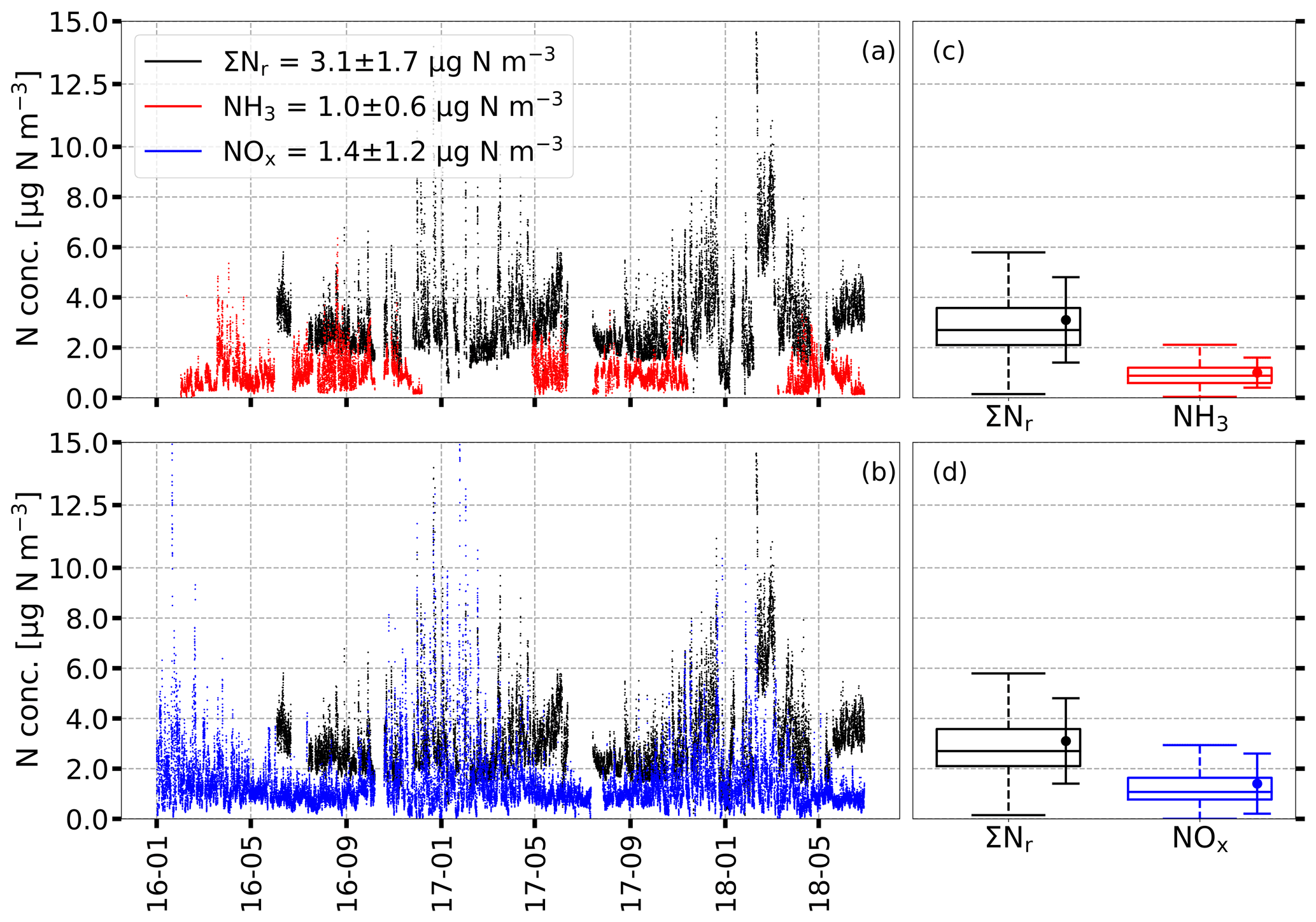
Figure 1Half-hourly averaged concentrations of ΣNr (black), NH3 (red), and NOx (blue) in µg N m−3 from 1 January 2016 to 30 June 2018 displayed in (a, b). Box plots (box frame = 25 % to 75 % interquartile range (IQR), bold line = median, whisker ) with average values (dots) shown in (c, d) refer to the entire campaign. Error bars represent 1 standard deviation. Y axis is capped at 15 µg N m−3.
ΣNr concentrations exhibited highest values during the winter months. For example, values were higher than 10 µg N m−3 during January 2017 and February 2018. NOx also showed a relatively high concentration level during winter. During spring and summer, NOx values were lower than 2 µg N m−3, and hence their contribution to ΣNr decreased. However, ΣNr values remained around 3 µg N m−3 and reached values of up to 6 µg N m−3, which was related to higher NH3 concentrations during these periods. The ΣNr concentration was 3.1 µg N m−3 on average, NH3 was 1.0 µg N m−3, and NOx was 1.4 µg N m−3 on average with the latter values being in agreement with concentrations reported by Beudert and Breit (2010). Averaged NH3 concentrations of the QCL agreed well with NH3 from passive samplers and DELTA measurements (Fig. S2 in the Supplement). Overall, the agreement in the annual pattern was reasonable, but a bias between the QCL and the diffusion samplers was found. From passive sampler measurements, an increase in the NH3 concentration with measurement height was observed. At 10 m (in the canopy), the lowest NH3 concentrations were measured. No systematic difference was found between 20 and 30 m. At 50 m, the NH3 concentration exceeded that at 30 m by 0.1 µg N m−3. During winter, the difference in measurement heights diminished.
The seasonal variations of the half-hourly ΣNr concentrations are represented by box-and-whisker plots including monthly medians in Fig. S3 in the Supplement. In general, median concentrations were comparable for the entire campaign with slight differences between the years. Medians ranged between 2 and 3.5 µg N m−3. From July to September, concentrations were slightly higher in 2016 than in 2017. During this period, interquartile ranges (IQRs) and whiskers were the smallest for the entire year showing less variability in ΣNr concentrations. In spring and winter, median concentrations were higher, and concentrations covered a wider range compared to the summer months. Figure S4 in the Supplement shows the corresponding diurnal patterns for each month. During the entire day, ΣNr concentrations exhibited variations of less than 1 µg N m−3. If concentrations were averaged for each season (not shown), higher concentrations were observed from 09:00 to 15:00 LT and lower values during the night.
Figure 2 shows absolute concentrations of individually measured Nr compounds as stacked bars and ΣNr from the TRANC from January 2016 to June 2018. TRANC and NOx measurements were averaged to exposure periods of DELTA measurements. DELTA measurements recorded at an insufficient pump flow were excluded from the analysis. Missing NH3 values in the DELTA time series were filled by NH3 data determined from the passive sampler mounted at 30 m. Remaining data gaps in the DELTA time series of NH3, HNO3, , and were replaced by monthly averages from other years.
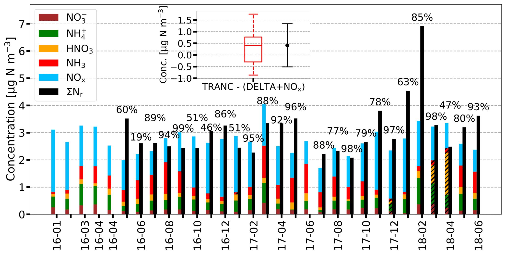
Figure 2Monthly stacked concentration of TRANC, DELTA, and NOx in µg N m−3 for the entire measurement campaign. Missing NH3 values from the DELTA measurements caused by a low pump flow were filled with passive sampler values from 30 m. This procedure was done for December 2016 and 2017, March 2018, and April 2018. Remaining gaps in the time series of HNO3, , and were replaced by monthly averages estimated from other years if possible. In the case of NH3, the procedure was applied to January 2017. For the other compounds, the gap-filling was done for December 2017, March 2018, and April 2018. Gap-filled bars are hatched. NOx and ΣNr were averaged to the exposure periods of the DELTA samplers. Numbers above the bars indicate the relative coverage of TRANC measurements during each exposure period.
The comparison of the TRANC with DELTA + NOx revealed overestimations by the latter from August 2016 to October 2016 and from January to March 2017. On average, an underestimation by DELTA + NOx of approximately 0.41 µg N m−3 with a standard deviation of 0.93 µg N m−3 was observed. The median value was about 0.4 µg N m−3.
HNO3, , and concentrations were nearly equal through the entire measurement campaign. Seasonal differences existed mainly for NH3 and NOx. We measured average concentrations of 0.55, 0.17, 0.42, 0.19, and 1.40 µg N m−3 for NH3, HNO3, , , and NOx for the entire campaign, respectively. On average, the relative contribution of NH3, HNO3, , and to ΣNr was less than 50 % for the entire measurement campaign as visualized by Fig. 3. We further observed a low particle contribution to the ΣNr concentrations (∼22 % on average) showing that the ΣNr concentration pattern was significantly influenced by gaseous Nr compounds.
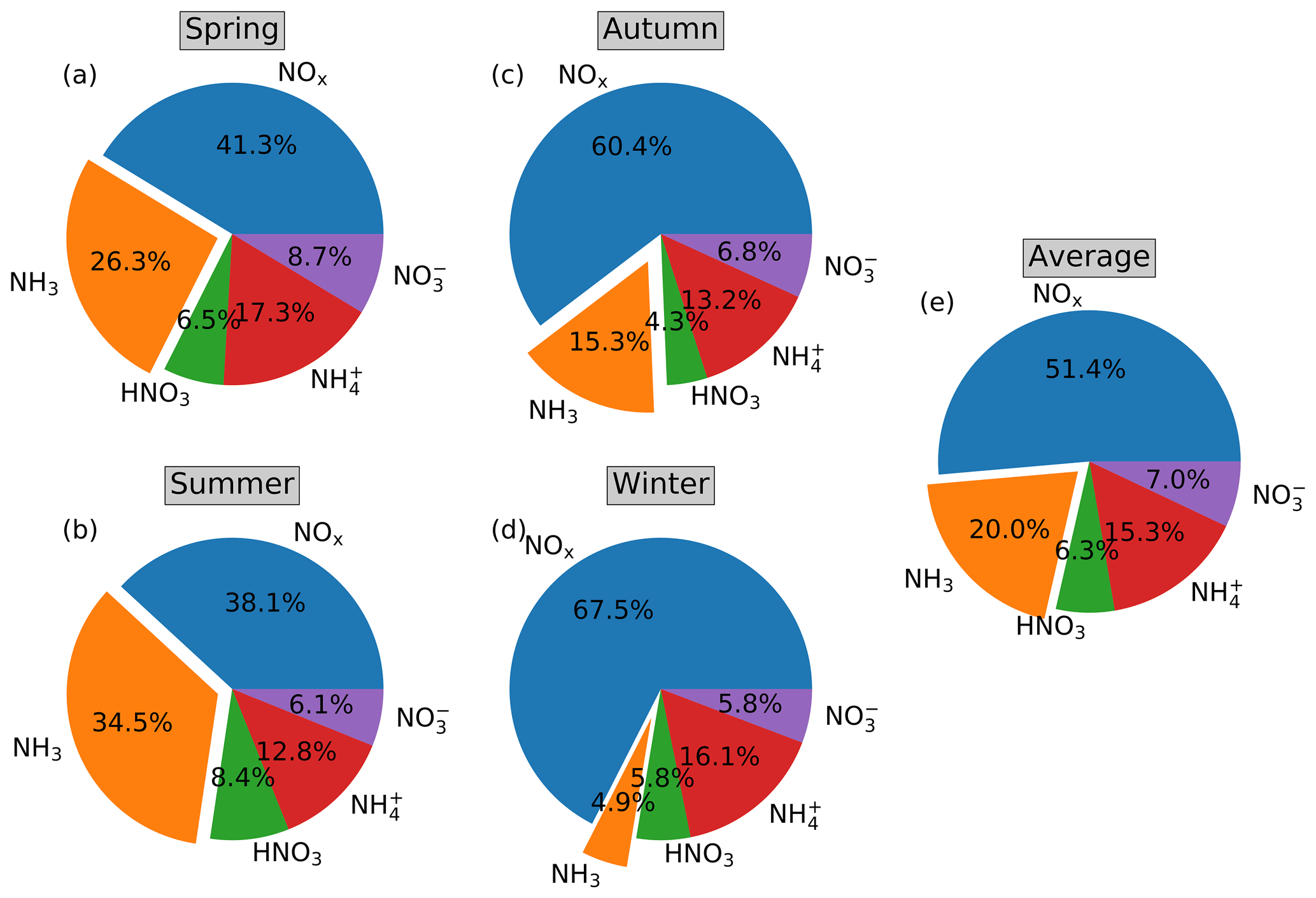
Figure 3Pie charts showing the relative contribution of concentrations for NOx, NH3, , , and HNO3 to ΣNr based on DELTA samplers and NOx measurements for different seasons of the year. NOx measurements are averaged to exposure periods of the DELTA samplers. Panels (a)–(d) refer to spring, summer, autumn, and winter, respectively. Panel (e) shows the average relative contribution to ΣNr for the entire measurement period.
In general, NOx showed the highest contribution to ΣNr and followed seasonal changes with highest values during winter and lowest values in summer. NH3 also featured seasonal variations with concentrations lowest in winter and highest values in spring and summer. Seasonal contributions of HNO3 varied by less than 2 % compared to the average. The highest relative contribution of HNO3 was found for summer. and exhibited highest values for spring. The excess of over is obvious. Similar to HNO3, the seasonal contribution of and deviated only by ±2 % from their averages. Only small seasonal changes in the overall ΣNr concentration were observed. As shown in Fig. 2, ΣNr concentrations were between 2 and 4.5 µg N m−3 excluding February 2018. We measured 3.3, 2.6, 2.5, and 3.0 µg N m−3 with the TRANC system for spring, summer, autumn, and winter, respectively.
3.2 Measured exchange fluxes and deposition velocities of ΣNr
Figure 4 shows the non-gap-filled ΣNr fluxes depicted as box plots on a monthly timescale. The convention is as follows: negative fluxes represent deposition, positive fluxes emission.
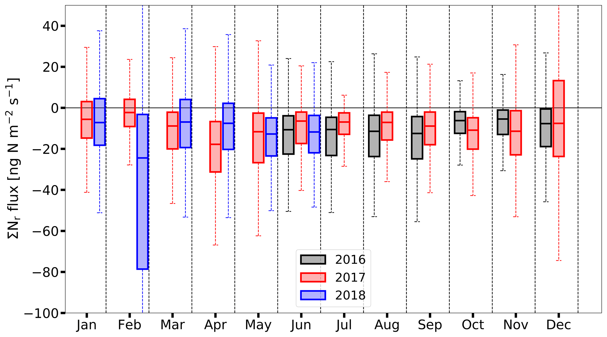
Figure 4Time series of measured high-quality (flags “0” and “1”) ΣNr fluxes depicted as box-and-whisker plots on a monthly basis (box frame = 25 % to 75 % interquartile ranges (IQR), bold line = median, whisker ) in . Colors indicate different years. The whiskers in February 2018 cover the range from −191 to 105 ; the upper whisker of December 2017 was at 69 .
Except for February 2018, all ΣNr flux medians were between −15 and −5 , indicating that deposition of ΣNr predominated at our measurement site. Quality-assured half-hourly fluxes showed 80 % deposition and 20 % emission fluxes. On a half-hourly basis, fluxes were in the range from −516 to 399 . On a monthly basis, random flux error medians were between 3 and 6 . According to Langford et al. (2015), the limit of detection (LOD) is calculated by multiplying the random flux error (95 % confidence limit) with 1.96. The comparison of half-hourly fluxes with their individual LOD revealed that 79 % of the measured fluxes were above their detection limits. Deposition fluxes contributed with 84 % to fluxes above the LOD. The fraction of emission was estimated to 16 %. The relative contribution of emission fluxes to measured fluxes decreased under the consideration of the LOD. This indicates that emission fluxes were closer to the flux detection limit of the instrument.
In general, median deposition was within the same range for the entire campaign with only small seasonal differences. For instance, median deposition was higher during spring and summer than during winter for 2016. However, median deposition during winter 2017 was comparable to median deposition in summer 2017. Median deposition was significantly increased from June 2016 till September 2016 compared to the same period in 2017, and IQR and whiskers also covered a wider range in 2016. The pattern changed for the time period from October to December. In December 2017, the IQR expanded in the positive range indicating emission events for a significant time period. The largest median deposition with 25 and the widest range in IQR reaching approximately −80 were registered in February 2018, indicating strong deposition phases during that month with sporadic emission events. Such phenomena were not observed in the years before. In the following month, the deposition was higher from March to April 2017 than for the same period in 2018. Figure 5 shows averaged diurnal cycles of measured ΣNr fluxes for every month.
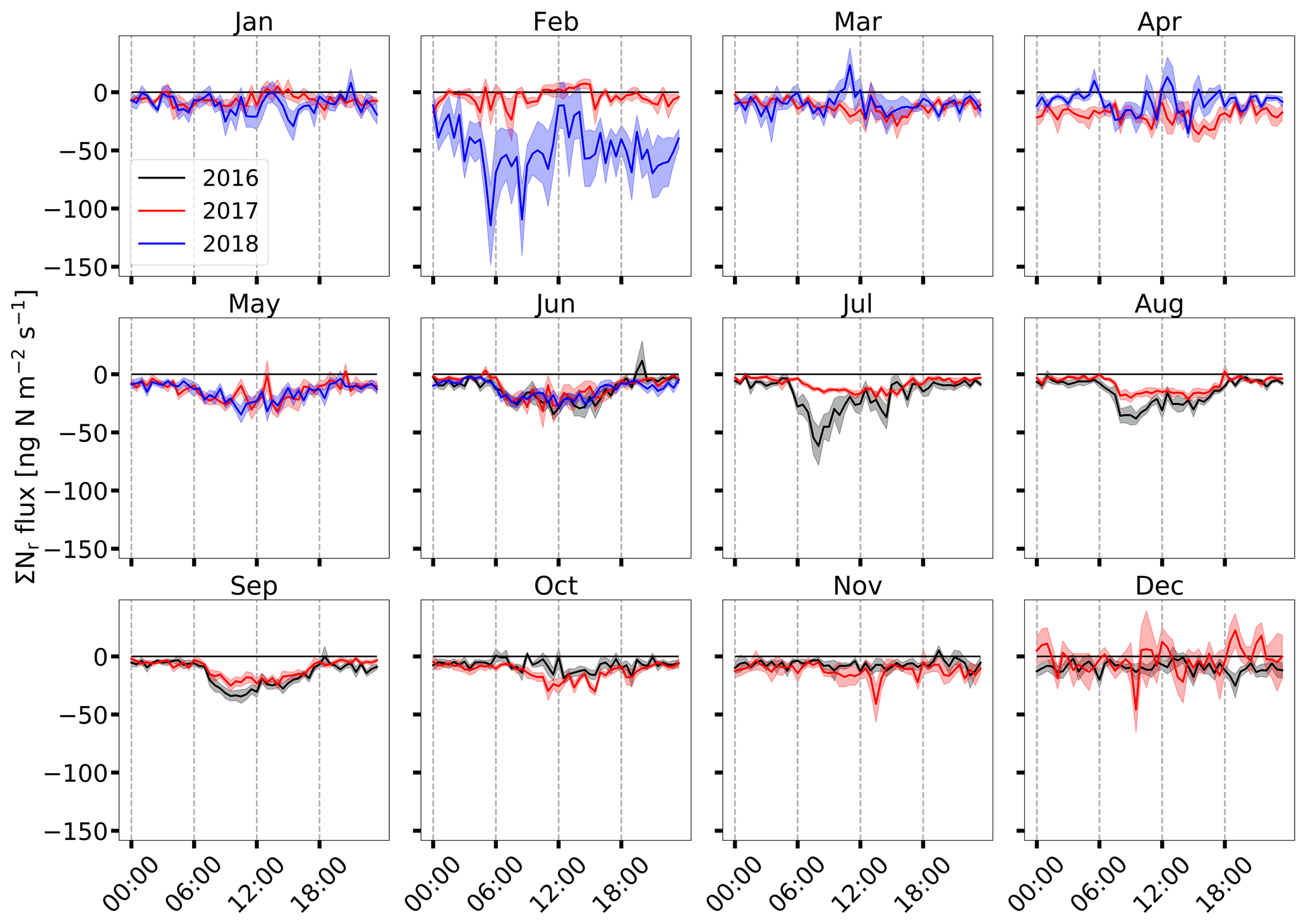
Figure 5Mean diurnal cycle of ΣNr fluxes () based on half-hourly measurements for every month from June 2016 to June 2018. The shaded area represents the standard error of the mean. Colors indicate different years.
In general, the ΣNr diurnal cycle exhibited low deposition or fluxes close to zero during nighttime/evening and increasing deposition during daytime. Deposition fluxes were similar during the night for the entire campaign except for February 2018. Maximum deposition was reached between 09:00 and 15:00 LT. Deposition is enhanced from May until September showing fluxes between −40 and −20 . From October to November and from December to February, the diurnal cycle weakened with near-zero or small negative fluxes, which were lower than −10 . The diurnal cycles of the respective same months were comparable. However, during certain months, which differ in their micrometeorology and/or in the composition of ΣNr, differences can be significant. For example, the diurnal cycles of March and April 2017 were clearly different to the diurnal cycles of March and April 2018. During spring 2017, deposition fluxes were found whereas the ΣNr exchange was close to zero one year later. The median deposition was also larger in March and April 2017 than in the year after (Fig. 4). In December 2017, the diurnal cycle was close to the zero line and positive fluxes were observed, although standard errors were relatively large (±11.5 on average). In December 2016, small deposition fluxes were observed for the entire diurnal cycle. The diurnal cycle of February 2018 showed highest deposition values during the entire day, even the highest values during the measurement campaign. Again, the average standard error was relatively large (±19.9 ) for February 2018 compared to February 2017.
Figure S5 shows the median vd for the corresponding fluxes. Values ranged between 0.2 and 0.5 cm s−1 for the entire campaign. In general, median vd followed closely the seasonality of their corresponding fluxes (Fig. 4). During autumn and winter, vd remained stable. From May to September, a continuous increase in vd was observed from 06:00 until noon. A decrease in vd followed in the late afternoon (15:00 to 18:00 LT). Similar to the diurnal fluxes, maximum vd values were reached between 09:00 and 15:00 LT. During that time, values of vd were close to 1 cm s−1 or even higher (Fig. S6).
3.3 Controlling factors of measured ΣNr deposition velocities
From May to September, a clear diurnal pattern was found for vd and their corresponding fluxes (Figs. 5 and S6). It was characterized by lower deposition during the night and highest values around noon (Fig. S9). During winter, deposition fluxes were close to zero and showed no diurnal variation leading to a constantly low vd except for midday (Fig. S10). During that time, a strong decrease in vd was found with near-zero or even small negative values around 12:00 LT. Micrometeorological parameters such as global radiation (Rg) (Zöll et al., 2019), temperature and turbulence (Wolff et al., 2010), humidity (Wyers and Erisman, 1998; Milford et al., 2001), dry/wet leaf surfaces (Wyers and Erisman, 1998; Wentworth et al., 2016), and the concentration of ΣNr, especially changes in the concentration of the individual nitrogen compounds (Brümmer et al., 2013; Zöll et al., 2016), were reported to control the deposition of ΣNr.
In order to investigate the influence of u∗ on the ΣNr exchange, Fig. S7 in the Supplement illustrates the dependency of vd on u∗ for deposition and emission fluxes during day and night. The Rg threshold for day and nighttime fluxes was set to 10 W m−2. For better visibility, we binned data in 0.1 m s−1 increments of u∗. Since bins are not equal in size, we added corresponding half-hourly fluxes to the plots. Red dots represent averages of each bin and error bars correspond to their standard error. We found that vd increased slightly with u∗ due to dependency of vd on Ra and Rb. The latter are proportional to the inverse of u∗, suggesting that the increase with u∗ should follow a power law. In the case of particles, linear relationships between u∗ and vd were found by Gallagher et al. (1997), Lavi et al. (2013), and Donateo and Contini (2014). Although uncertainties of the binned averages were large, a relationship between vd and u∗ seems to exist as suggested by the correlations (r), but no clear functional relationship could be identified due to the large scattering of half-hourly vd.
For visualizing the impact of the concentration on vd (Fig. 6), we plotted the ΣNr concentration against the ratio in order to reduce the influence of Ra and Rb on vd. The threshold for Rg was set to 10 W m−2, and we binned data in 0.5 µg N m−3 increments of the ΣNr concentration.
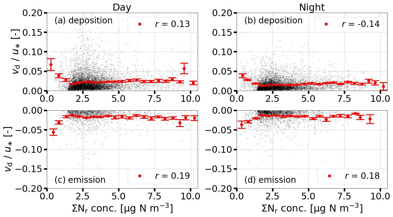
Figure 6Relationships between measured ΣNr concentrations and corresponding ratios separated in emission and deposition during day (a, c) and night (b, d). Half-hourly data are displayed in black; red dots represent averages binned in increments of 0.5 µg N m−3. Error bars indicate the standard error of the averages. The threshold for identifying day and nighttime vd was set to 10 W m−2. r represents the measure of correlation evaluated for the binned data.
It is obvious that exhibited no significant dependence on the ΣNr concentration as shown by the low values for r. The ratio appeared to be constant across the (entire) concentration range. It demonstrates that the ΣNr concentration had no significant influence on their vd. In the case of particles, the ratio depends on Obukhov length (L) and particle size according to Gallagher et al. (1997) and Lavi et al. (2013). In the case of deposition fluxes measured during daytime, we found that the ratio decreased for up to a minimum if L−1 reaches zero (neutral stratification) (Fig. S8 in the Supplement). This relationship was observed by Gallagher et al. (1997) and Lavi et al. (2013). Although the scattering of half-hourly ratios is large, the decrease of the ratio with increasing L−1 and the dependence of vd on u∗ demonstrate that vd was more influenced by micrometeorological variables than by the ΣNr concentration.
From the analysis of Figs. 6, S7, and S8, it is impossible to state u∗ or L as the controlling variable of the ΣNr exchange since turbulence, stratification, Rg, sensible heat flux, air temperature, and relative humidity are highly correlated with each other. Figure S9 shows the diurnal cycle of concentration, Rg, u∗, air temperature (Tair), and vd for the period from May to September. During that period, a clear diurnal pattern in vd was observed with largest values around noon and lowest values during the night. During winter (December, January, and February) (Fig. S10), vd was almost equal and even lower during the day, which resulted in a lower deposition of ΣNr during winter. The different shapes of the diurnal variations of vd could be induced by micrometeorological variables, which change the composition of available ΣNr compounds during the day (e.g., Munger et al., 1996; Horii et al., 2004, 2006; Wyers and Duyzer, 1997; Van Oss et al., 1998) and promote photosynthesis (e.g., stomatal uptake or release of NO2 Thoene et al., 1996 and NH3 Wyers and Erisman, 1998).
Within the period of enhanced ΣNr exchange, in particular from May to September, we investigated the dependency of the ΣNr deposition velocities on Tair, relative humidity (RH), dry/wet leaf surface, and ΣNr concentration. We separated half-hourly vd into groups of low and high Tair, RH, and concentration according to their median. In the case of separating vd into groups of dry and wet leaf surfaces, we used the proposed calculation scheme of a leaf wetness Boolean (see Sect. 2.2). No significant influence of the different installation heights on leaf surface wetness was found (see Fig. S11 and corresponding description in the Supplement). Figure 7 shows the results for vd.
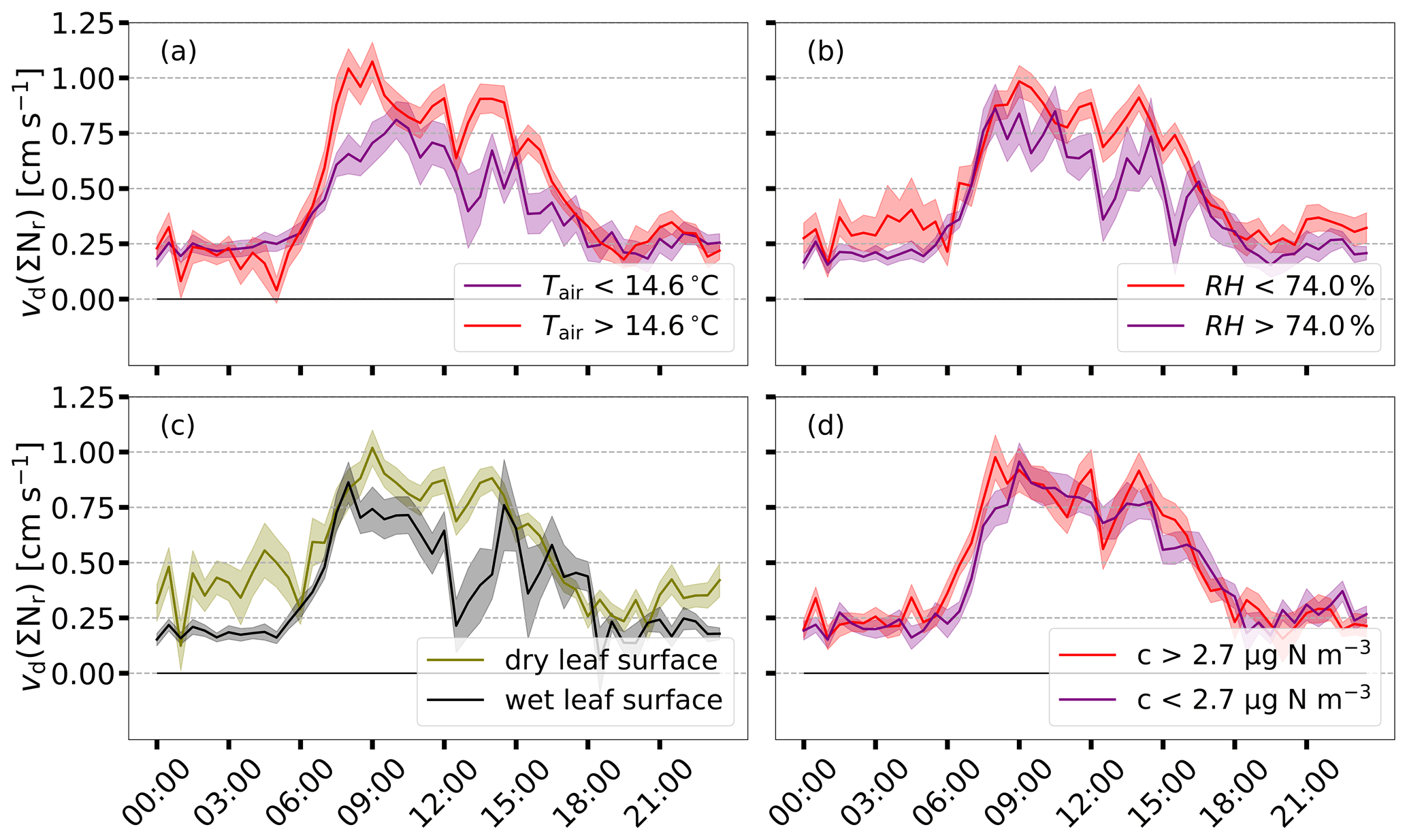
Figure 7Mean diurnal cycle of vd from May to September for low and high temperature (a), relative humidity (b), and concentration (c). Median values of temperature, humidity, and concentration, which are derived for the same time period, are used as threshold values for separating vd. In panel (d), the mean diurnal cycle of vd for dry and wet leaf surfaces is shown. For classifying leaf surfaces as dry or wet, the scheme proposed in Sect. 2.2 is applied. The shaded areas represent the standard error of the mean.
In general, higher air temperatures, lower relative humidity, and dry leaf surfaces were associated with enhanced deposition of ΣNr, and a clear diurnal pattern was observed for vd with high values around noon and low, non-zero values in the night. During dawn/nighttime, deposition velocities exhibited no significant difference between the applied temperature and humidity thresholds. In the presence of dry leaf surfaces, vd was higher by approximately 0.2 cm s−1 compared to wet leaf surfaces during the night. During the entire day, no difference was found for low and high concentration regimes. During other times of the year, no diurnal pattern was observed. In those periods, vd was almost constant and exhibited lower values during daylight compared to the May to September period. Occasionally, negative deposition velocities referring to emission of ΣNr were recorded during times of lower radiation.
3.4 Dependence of ΣNr dry deposition sums on micrometeorological variables
We found that preferentially micrometeorological variables enhance deposition velocities and fluxes. The application of data-driven gap-filling methods like MDV (Falge et al., 2001) for estimating dry deposition could lead to biased results if micrometeorological conditions of the certain gap are different to fluxes used for filling the gap. Therefore, we determined dry deposition budgets with and without u∗ filter and conducted gap-filling with additional conditions for temperature, relative humidity, and wind speed.
Figure 8 shows the non-gap-filled ΣNr fluxes depicted as box plots and their cumulative sums with and without a u∗ filter if OMDV is used as a gap-filling approach. For details to the implementation of OMDV, we refer to Sect. 2.3.

Figure 8Panel (a) shows the non-gap-filled ΣNr fluxes represented by box-and-whisker plots with (red) and without (black) u∗ filter in (box frame = 25 % to 75 % interquartile ranges (IQR), bold line = median, whisker ). The threshold for u∗ was set to 0.1 m s−1. In panel (b), the cumulative dry deposition of ΣNr is plotted for both cases in kg N ha−1. For determining the cumulative curves, OMDV was used as a gap-filling method, and gaps were filled with fluxes being in a range of ±5 d. Remaining gaps were not filled. In the legend of panel (b), cumulative ΣNr deposition and the total uncertainty of the gap-filled fluxes according to Eq. (3) (see Sect. 4.3) are shown.
The difference in dry deposition was approximately 400 g N ha−1 after 2 years and corresponds to 6 % of the cumulative sum with u∗ filter. Figure 8a shows that median deposition of ΣNr with u∗ filter was equal to or larger than the median deposition without u∗ filter. Thus, the applied u∗ threshold removed not only small fluxes resulting in a consistent bias between the median deposition. The contribution of the water vapor correction (Eq. 1) to the estimated dry deposition was very low. ΣNr interference fluxes were between −3 and −0.3 . The uncertainty ranged between 0.0 and 0.5 . Considering 2 years of TRANC flux measurements with OMDV as a gap-filling approach, the correction contributed with 131 g ha−1 to the estimated dry deposition of 6.7 kg ha−1.
In order to evaluate the influence of micrometeorological variables such as temperature (T), RH, and wind speed (wsp) on annual ΣNr dry deposition, we compared the deposition estimates of OMDV with CMDV in regard to the measurement years from the beginning of June to the end of May (Fig. 9). Details about the implementation of CMDV are given in Sect. 2.3.
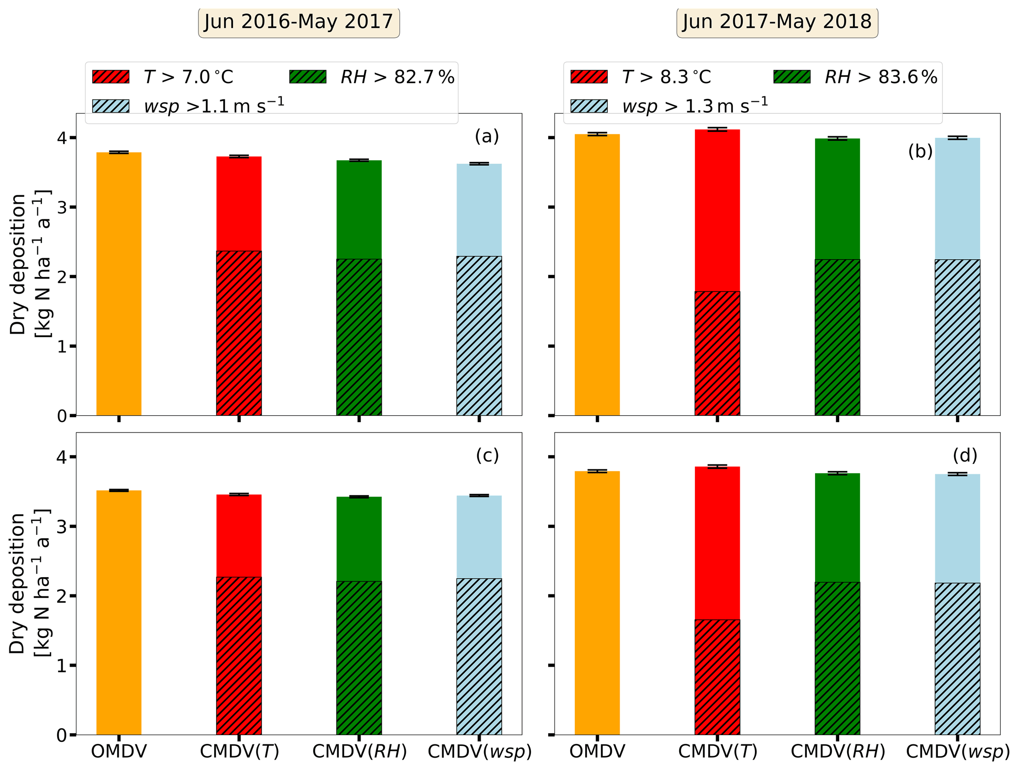
Figure 9Annual ΣNr dry deposition shown as bar graphs from June to May in . For the orange bar, short-term gaps were filled with the OMDV approach while using only fluxes in the time frame of ±5 d. In the case of the red, green, and blue bars, the CMDV approach is applied for temperature (T), relative humidity (RH), and wind speed (wsp), respectively. Fluxes used for CMDV have to additionally be in a range for T (), RH (±5 %), or wsp (±1.5 ms−1). For OMDV and CMDV, remaining gaps were replaced by monthly averages estimated for each half-hour calculated from the non-gap-filled fluxes. Panels (a, b) were made for fluxes with u∗ filter, (c, d) without it. The hatched area of the bars represents the dry deposition for T, RH, and wsp values higher than the annual median shown in the legend. Error bars correspond to the total uncertainty of the gap-filled fluxes (see Eq. 3).
No significant difference could be found between the dry deposition sums and their cumulative uncertainties related to gap-filling for both measurement years. Consequently, the applied selection criteria did not lead to biased sums compared to the dry deposition calculated with OMDV. The relative contribution to dry deposition related to temperatures, relative humidity, and wind speeds above their respective medians was at 60 % and at 55 % in the first and second measurement year, respectively. As shown before, a difference in the application of a u∗ filter exists but is within the uncertainty range. Dry deposition was higher in 2017/2018, which was related to the large deposition fluxes observed in February 2018. Still, differences between the years were within their uncertainty ranges. In total, we estimated 3.8 and 4.0 with the OMDV approach (orange bar) and u∗ filter for 2016/17 and 2017/18, respectively.
3.5 Wet and total nitrogen deposition
Wet deposition was estimated from measurements of bulk and wet-only samplers. Table 1 shows estimated ΣNr dry depositions, the deposition estimates of -N, –N, dissolved organic nitrogen (DON), and the resulting total nitrogen from wet deposition (TWD) for all seasons and both measurement years. Please note that the sum of all seasons corresponds to the sum of both measurement years.
Small seasonal and annual differences in dry deposition were determined (approx. 200 g N ha−1 per period). Total seasonal and annual uncertainties related to gap-filling (Eq. 3) were between 7 and 21 g N ha−1 per period. Dry deposition contributed approximately one-third to total deposition except for winter (Fig. S12). In the second year, the contribution of dry deposition was higher than in the first year. Higher fractions of dry deposition were related to the large dry deposition occurring in late February 2018. Thus, dry deposition and its uncertainty were remarkably high during winter. Total wet deposition (TWD) was highest in spring and summer (Figs. 2 and S2). During those periods, –N contributed most to TWD, which was probably related to high NH3 concentrations. Interseasonal differences for –N were found but were lower compared to changes in –N. DON deposition was lowest and was between 0.1 and 0.6 . Overall, differences in TWD for both sampler types were less than 300 except for winter. Total wet + dry deposition was equivalent to 12.2 for 2016/17 and 10.9 for 2017/18.
4.1 Interpretation of measured concentrations and fluxes
Measured half-hourly ΣNr concentrations were low relative to sites exposed to agricultural activities or urban environments. On average, we measured 5.5 ppb (3.1 µg N m−3) ΣNr, 1.8 ppb (1.0 µg N m−3) NH3, and 2.5 ppb (1.4 µg N m−3) NOx. Wintjen et al. (2020) determined an average ΣNr concentration level of 21 ppb (12 µg N m−3) for a seminatural peatland, Brümmer et al. (2013) measured between 7 and 23 ppb (4 and 13 µg N m−3) as monthly averages above a cropland site, and Ammann et al. (2012) measured half-hourly ΣNr concentrations ranging from less than 1 to 350 ppb (0.6 to 201 µg N m−3) for a grassland site. Only for certain time periods, ΣNr concentrations reached significantly higher values. During winter, NOx increased due to emission from heating with fossil fuels and from combustion processes, for example through traffic and power plants. A generally lower mixing height, which is often observed during winter, also leads to higher ground-level concentrations of air pollutants. In spring and autumn, higher ΣNr concentrations can be attributed to NH3 emission from the application of fertilizer and livestock farming in the surrounding environment (Beudert and Breit, 2010). NH3 emissions from livestock farming in rural districts around the NPBW are approximately half of the emissions compared to rural districts located in the Danube–Inn valley (Beudert and Breit, 2010). The authors measured concentrations of NO2 (2.1–4.8 ppb (1.2–2.8 µg N m−3)), NO (0.4–1.6 ppb (0.2–0.9 µg N m−3)) and NH3 (1.4 ppb (0.8 µg N m−3)) at the same site. Those values for NO2 and NO refer to 1992 until the end of 2008; NH3 was measured from mid-2003 to 2005. The low concentration level and seasonal variability of the ΣNr compounds, in particular NH3 and NO2, are in agreement with Beudert and Breit (2010). Low concentration values of NH3 and NOx are reasonable for a site, which is some kilometers away from anthropogenic emission sources. Studies like Wyers and Erisman (1998), Horii et al. (2004), and Wolff et al. (2010) conducted measurements of NH3 and NO2 above remote (mixed) forests and reported similar concentrations for those gases.
Our measurements further indicated that NOx made the highest contribution to the measured ΣNr concentrations. At the measurement height, the contribution of NO to NOx was negligible. Median contribution of NO to NOx concentrations was approximately 10 % at 50 m. NO exhibits higher concentrations and fluxes close to the forest floor as shown by Rummel et al. (2002). Even if soil NO was converted to NO2 it could still contribute to the measured ΣNr flux except for the fraction that is removed by the canopy. As mentioned in Sect. 2.2, NO2 concentrations had been measured at 50 m. Seok et al. (2013) reported marginal differences in NO2 concentrations above the canopy at a remote site. Above the canopy, height differences in NO2 concentrations were probably not relevant for the measurement site. The NOx analyzer was equipped with a thermal converter and likely cross-sensitive to other NOy compounds. However, measured concentrations of HNO3 or were comparatively low as seen in Fig. 2. Thus, their influence on NOx measurements was most likely small. In the context of height differences, we found no systematic difference between NH3 concentrations within the canopy and just above the canopy. Only for short time periods, for example in summer 2016 and 2017, differences in passive samplers were found indicating a small NH3 flux. Considering the LOD of IVL passive samplers for NH3 of 0.4 µg N m−3 determined by Dämmgen et al. (2010) shows that passive sampler measurements were conducted close to their LOD. It suggests that the uncertainty of the passive samplers was too large to resolve flux gradients. Still, NH3 had a strong presence in the ΣNr concentration within the growing period of the plants, in particular during spring and summer. DELTA measurements further suggested that the ΣNr concentration pattern was mainly influenced by gaseous Nr.
The increase in the relative contributions of HNO3 from spring to summer compared to the decrease of and (Fig. 3) can be related to the evaporation of NH4NO3 (Wyers and Duyzer, 1997; Van Oss et al., 1998; Schaap et al., 2002). However, the findings of Tang et al. (2015) and Tang et al. (2021) revealed that HNO3 concentrations measured by the DELTA system using carbonate coated denuders may be significantly overestimated (45 % on average) since HONO sticks also at those prepared surfaces. Thus, the measured HNO3 concentrations should be seen as an upper estimate. Due to the reaction of NH3 with HNO3 and sulfuric acid particulate is formed, available as (NH4)2SO4 or NH4NO3 (Trebs et al., 2005).
These aerosols are mainly in the fine mode and associated with aerodynamic diameters less than 2.5 µm (PM2.5) (Kundu et al., 2010; Putaud et al., 2010; Schwarz et al., 2016). Since the DELTA cut-off size is approximately 4.5 µm (Tang et al., 2015), fine accumulated particles could be adequately detected. Coarse-mode aerosols like sodium nitrate (NaNO3) are formed in the presence of sea salt (Na+ and Cl−) or other geological minerals or biological particles like pollen (Lee et al., 2008; Putaud et al., 2010). Generally, concentrations of Na+, Ca2+, and Mg2+ were close to zero during the entire campaign. On average, we measured 0.08 µg m−3 for Na+ and 0.01 µg m−3 for Ca2+ and Mg2+. Although these concentrations were close to and lower than the LOD of DELTA (Tang et al., 2021) and partly underestimated by the filters of the DELTA system due to the cut-off size of approximately 4.5 µm, it illustrates that coarse-mode nitrate levels are not expected to be significant at the measurement site. As noted in Sect. 2.2, cellulose filters were used for collecting and SO. According to Tang et al. (2015), cellulose filters underestimate and SO ions, sulfate by 11 %, and nitrate by 37 %. However, Schaap et al. (2004) found that cellulose filters are appropriate for capturing . Inside of the TRANC, high temperatures (≥870 ∘C) probably led to a chemical decomposition of coarse aerosols (Yuvaraj et al., 2003). Marx et al. (2012) found that the TRANC is able to convert NaNO3. Thus, we assume that the TRANC's cut-off size was higher resulting in a higher sensitivity to aerosols in the coarse mode. Still, we observed a clear excess of over . Presumably, the contribution of aerosols to TRANC measurements was not significant. In addition, higher oxidized compounds like N2O5 or peroxyacetyl nitrates could not be collected by DELTA but were probably converted by the TRANC. Issues in the temperature stability or CO supply leading to instabilities in the conversion efficiency of the TRANC may be responsible for disagreements to the collection efficiency of the denuders. A key uncertainty was the data coverage of the TRANC, which was 78 % on average during the exposure periods. In total, the comparison of the total N concentrations shows that the TRANC can adequately measure ΣNr concentration.
In general, a comparison of ΣNr concentrations and fluxes to other studies is difficult due to the measurement of the total nitrogen. Most studies that have been published so far focused only on a single or a few compounds of ΣNr and are limited to selected sites and time periods of a few days or months. Only a few studies had been focusing on ΣNr flux measurements using the EC method (see Ammann et al., 2012; Brümmer et al., 2013; Zöll et al., 2019; Wintjen et al., 2020). Brümmer et al. (2013) measured ΣNr exchange above an agricultural land. During unmanaged phases, fluxes were between −20 and 20 . Apart from management events, fluxes above the arable field site were closer to zero compared to our unmanaged forest site, which is dominated by deposition fluxes and is therefore a larger sink for reactive nitrogen. Ammann et al. (2012) measured ΣNr fluxes above a managed grassland. In the growing season, deposition fluxes of −40 were measured. The authors reported increased deposition due to weak NO emission during that period. Similar to Brümmer et al. (2013), the flux pattern observed by Ammann et al. (2012) is influenced by fertilizer application and thus, varying contributions of Nr compounds, for instance by bidirectionally exchange of NH3 leading to both periods of net emission and deposition of ΣNr. Despite the low signal-to-noise ratio of emission fluxes and data coverage of 50 % from June 2016 to June 2018 at the measurement site, we were able to investigate the exchange pattern of ΣNr and could estimate reliable dry deposition sums. To our knowledge, flux measurements of ΣNr above mixed forests have not been carried out so far. We found that the flux magnitude and diurnal flux pattern were similar to observations reported for individual Nr species above forests, e.g., NH3 (Wyers and Erisman, 1998; Hansen et al., 2013, 2015), NO2 (Horii et al., 2004; Geddes and Murphy, 2014), HNO3 (Munger et al., 1996; Horii et al., 2006), and total ammonium (tot-) and total nitrate (tot-) (Wolff et al., 2010). As seen by the flux values and measurements of individual compounds, deposition prevails in the reported flux pattern, which corresponds to our measurements.
However, under certain circumstances regarding micrometeorology or the availability of ΣNr compounds large deposition or emission fluxes can be observed. In February 2018, remarkably high ΣNr concentrations and depositions were measured. During the exposure period of the DELTA samplers, we found 0.96, 0.17, 0.37, 0.27, and 1.70 µg N m−3 for , NH3, , HNO3, and NOx, respectively. The aerosol concentrations were exceptionally large in February 2018, which have affected these averages considerably. Averaged concentration during winter excluding February 2018 was only 0.38 µg N m−3 in comparison to 0.96 µg N m−3 for February 2018. The concentration in this month results in a concentration 2.5 times higher than the average. Also, the SO2 concentration was much larger (1.54 µg N m−3) in this month compared to the other winter months (0.37 µg N m−3). Figure 10 shows the relative contributions of each Nr compound for February 2018 compared to averaged fractions during winter excluding February 2018.

Figure 10Relative contribution of concentrations for NOx, NH3, HNO3, , and to ΣNr estimated from DELTA and NOx measurements for winter and separately for February 2018. NOx measurements are averaged to exposure periods of the DELTA samplers.
During February 2018, made a significant contribution to the ΣNr concentration. The measured value is an integrated value over approximately one month. Thus, daily contributions of could have been even higher. Earlier studies by, e.g., Wolff et al. (2010) report events with large aerosol deposition. During their campaign, wind speeds were relatively high. Largest aerosol deposition occurred during dry conditions, e.g., low RH, no rain, and high visibility. Figure S13 shows micrometeorological parameters, deposition velocities, and gap-filled ΣNr fluxes from the 12 February to 6 March. Large deposition fluxes were accompanied by high wsp and u∗ values, high Rg indicating high visibility, and low RH. The observed conditions are typical for cold air streams with high aerosol loads coming from northeast and led to a reduction in turbulent resistances resulting in a high vd, which is due to efficient turbulent mixing. Hence, even at low concentrations of significant aerosol deposition is possible if Ra and the surface resistance are reduced. In conclusion, particulate was mainly responsible for the large ΣNr deposition due to its excess over aerosol . Since we had no high-resolution flux measurements of any ΣNr compound, we have no evidence which aerosol predominated the ΣNr flux.
In December 2017, large emission fluxes were measured. Compared to 2016, significant differences in temperature and snow depth were observed. Figure 11 shows recorded temperature, snowfall, concentrations, and estimated fluxes of ΣNr from 6 to 15 December for 2016 and 2017. Here, ±3 d was chosen for filling the gaps in order to keep the short-term variability of the fluxes.
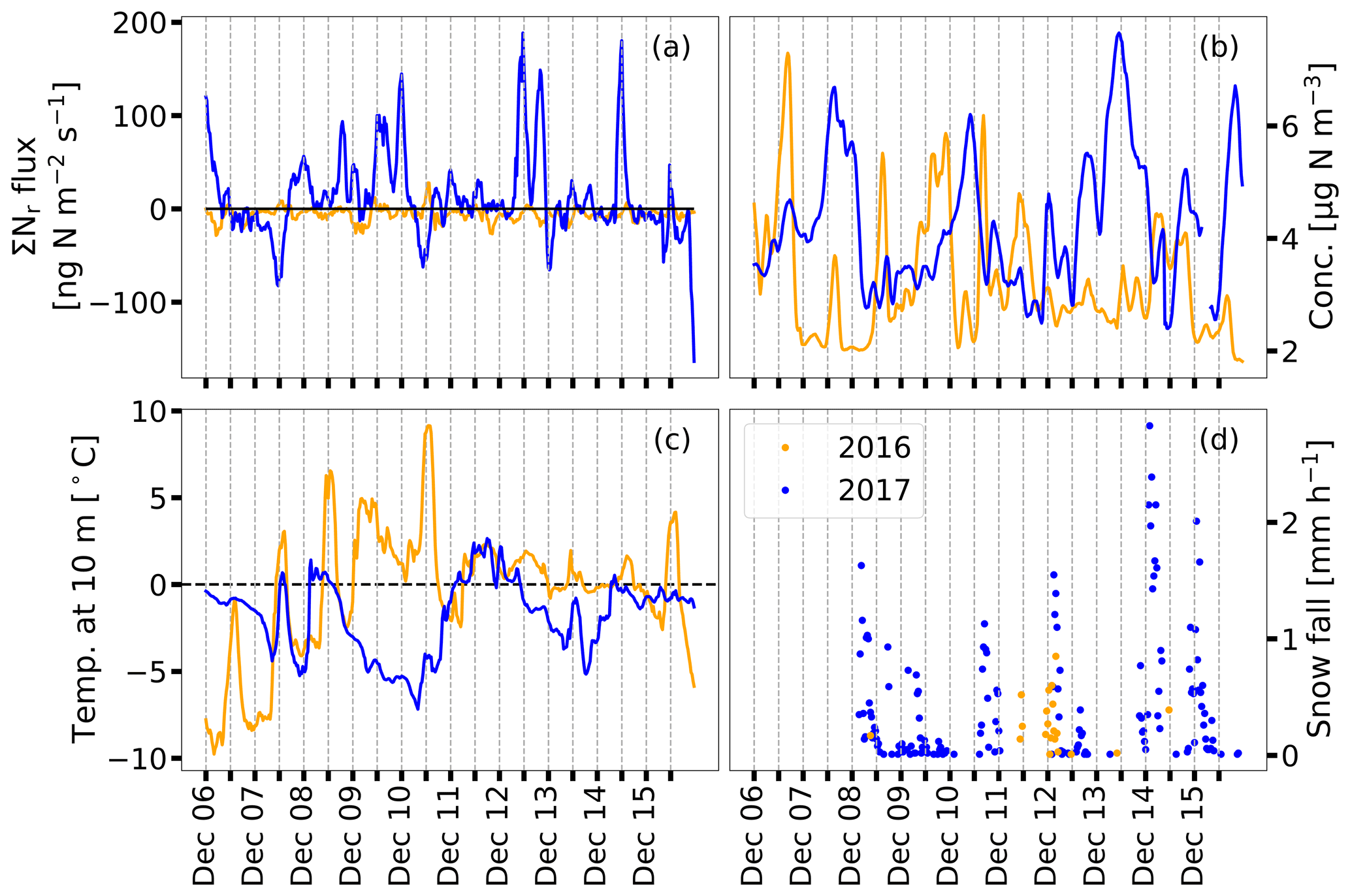
Figure 11ΣNr gap-filled fluxes (a), ΣNr concentrations (b), air temperature at 10 m height above ground (c), and snowfall (d) from 6 to 15 December for 2016 (orange) and 2017 (blue). Gaps are filled with the OMDV approach with fluxes being in a range of ±3 d. Fluxes and concentrations of ΣNr were smoothed with a 3 h running mean for better visualization.
In 2017, we observed substantial snowfall and a more slowly varying temperature compared to 2016, leading to significant snow depths compared to 2016. On the 1 December, 1 and 20 cm snow depth were measured in the fetch of the tower for 2016 and 2017, respectively. Two weeks later, snow depth increased to 5 and 60 cm, respectively. In addition, temperatures alternated around 0 ∘C with minimum and maximum values close to ±10 ∘C in December 2016. In 2017, temperatures were below 0 ∘C and only for one day above 0 ∘C, and global radiation was below 100 W m−2.
The decomposition of organic matter, e.g., leaves, occurring on the topsoil could be responsible for the observed ΣNr emission fluxes. Due to the large snow depth in December 2017, the snow pack could act as an isolator, inhibit soil frost penetration, and therewith promote decomposition processes. In December 2016, decomposition rates were likely reduced compared to 2017 since snow depth was smaller (e.g., Bokhorst et al., 2013; Kreyling et al., 2013; Saccone et al., 2013). The influence of snow cover on soil emissions of Nr compounds, for example NO, is still under discussion (Medinets et al., 2016). As stated by the authors, different results had been published about the origin of NO emissions from snow-covered soils (see Medinets et al., 2016, and references therein). Since we conducted no measurements of NO close to or at the forest floor, we were not able to examine the influence NO emissions from soil or snow on the ΣNr measurements. Since soil-emitted NO is rapidly converted to NO2 (Rummel et al., 2002), the measured ΣNr emissions were unlikely to be solely caused by NO. The low correlations of the ΣNr fluxes to micrometeorological variables could be related to, for example, time shifts between exchange processes and micrometeorological variations, multiple (chemical) interactions between the Nr compounds, and feedback mechanisms, which are difficult to quantify.
4.2 Influence of micrometeorology and nitrogen concentrations on deposition and emission
Figures S9 and S10 show that the variability of vd and other micrometeorological variables were highly correlated with each other. Thus, we could not examine the mechanistic micrometeorological driver of the ΣNr flux. The dependencies on u∗ or L (Figs. S7 and S8) could also be related to effects of sensible heat flux, Rg, or Tair. Surely, micrometeorological parameters such as Rg and Tair promote photosynthesis of plants (Jarvis, 1976), i.e., lower the stomatal resistance, which is essential for the stomatal uptake of ΣNr compounds such as NO2 (e.g., Thoene et al., 1996) and NH3 (e.g., Wyers and Erisman, 1998). Stomatal uptake of Nr compounds was possible during periods of photosynthetic activity, leading to high values of vd during the summer months (Fig. S9). Figure S10 reveals that a certain degree of ΣNr uptake still occurred in winter, but deposition decreased strongly during midday, and even periods of emission were observed. These emissions may be due to the decomposition of leaves, leading to a release NH3 in late autumn/early winter (Hansen et al., 2013), or from snow-covered soils (see Sect. 4.1).
The analysis of Fig. 6 revealed that deposition velocities were independent of the ΣNr concentration. However, the impact of increasing concentrations on nitrogen (deposition) fluxes is well documented, for example, by Ammann et al. (2012) and Brümmer et al. (2013) for ΣNr above grassland and arable land, respectively, by Horii et al. (2006) for NOy and Horii et al. (2004) for NOx above a mixed forest, and by Zöll et al. (2016) for NH3 above a seminatural peatland.
Since we had no possibility to determine the actual contribution of the individual compounds to the ΣNr flux, comparing micrometeorological dependencies of vd to observations made for individual compounds is not possible. In the case of NH3, surface wetness was identified as a controlling factor for the NH3 uptake in previous studies (Wyers and Erisman, 1998; Milford et al., 2001; Wentworth et al., 2016). For total ammonium and total nitrate (tot- and tot-, respectively), Wolff et al. (2010) found that tot- exchange was nearly zero and emission was observed for tot- during rain or fog. Highest deposition was observed during sunny days. For the actual compound mix at our measurement site, high temperatures (>14.6 ∘C), low relative humidity (<74.0 %), and dry leaf surfaces were found to enhance the surface uptake of ΣNr from May to September. Since the actual composition of the ΣNr flux is not known, no arguments about an agreement or disagreement to the cited publications can be made.
We further found that the ΣNr concentration did not change significantly through the year. The difference between lowest and highest seasonal concentration means was only 0.8 µg N m−3. However, DELTA measurements demonstrated that the contribution of individual compounds does show a seasonal cycle. Since the ΣNr compounds differ in their vd, the observed seasonality in the dry deposition flux is related to the availability of ΣNr compounds. For example, in spring and summer, NH3 had probably the largest contribution on the ΣNr flux. Elevated NH3 concentrations were likely caused by emissions from agricultural management in the surrounding region (Ge et al., 2020). The concentration of NH3 was still lower than of NO2, but the vd of NH3 is significantly higher than of NO2 for woodland. Deposition velocities of NH3 range between 1.1 and 2.2 cm s−1 (see Schrader and Brümmer, 2014, and references therein), and values between 0.015 and 0.51 cm s−1 were reported for NO2 (e.g., Rondon et al., 1993; Horii et al., 2004; Breuninger et al., 2013; Delaria et al., 2018, 2020). However, variations in the composition of ΣNr may correlate with micrometeorological parameters. For example, the formation of HNO3 is correlated with Rg. The solar radiation responsible for the stomatal opening also promotes the formation hydroxyl radicals, which react with NO2 to form HNO3 (e.g., Munger et al., 1996; Horii et al., 2004, 2006; Seinfeld and Pandis, 2006). Tair influences the diurnal pattern of NH4NO3, which may also volatilize close to the surface due to the depletion of its precursors and in the case the temperature gradient is large enough (Wyers and Duyzer, 1997; Van Oss et al., 1998). Thus, part of the and in the aerosol phase may be converted to NH3 and HNO3, which deposits faster to surfaces than aerosols. For tot- and tot-, mean vd of 3.4 and 4.2 cm s−1 were determined by Wolff et al. (2010). In the case of HNO3, mean values between 2 and 8 cm s−1 were published by Pryor and Klemm (2004), Horii et al. (2006), and Farmer and Cohen (2008).
In conclusion, the variability in micrometeorological controls such as Rg, Tair, u∗, or RH in combination with changes in ambient concentration levels of the ΣNr compounds explains the observed variation in the ΣNr flux pattern.
4.3 Uncertainties in dry deposition estimates
Fluxes determined with the EC method are exposed to systematic and random errors. Systematic errors are related to the design of the measurement setup and the instruments, data processing steps including calibration, tilt correction, detrending, and corrections due to low- and high-frequency attenuation (Wintjen et al., 2020), and advection fluxes originating preferentially from non-homogeneous surfaces. Uncertainties from the measurement setup were likely caused by an insufficient pump performance, issues in temperature stability of the TRANC and CLD, sensitivity loss of the CLD, and problems in the O2 and CO supply. Therefore, regular maintenance and continuous observation of instrument performance parameters such as TRANC temperature and flow rate were made. With manual screening of measured half-hourly values and the recording of these parameters, low-quality half-hourly values were effectively excluded from analysis. A basic assumption for the EC method is that the terrain needs to be flat, and the canopy height and density should be uniform (Burba, 2013). These site criteria are not perfectly fulfilled at our measurement site. The site is located in a low mountain range, and tree density is rather sparse south of the flux tower. Such diverse terrain characteristics could lead to unwanted turbulent fluctuations (non-stationarity of time series), which introduce noise in the cross-covariance function. A 2D-footprint analysis exemplarily made for the year 2016 showed that the 70 % isoline of the flux had an extension of approximately 300 m. In southwest direction of the tower (approx. distance 100 to 300 m), tree density and height were lower than to the northeast of the tower. Due to the high surface roughness, the flux footprint is limited in its size but the footprint represents the typical forest structure of the NPBW. Thus, we did not filter half-hourly fluxes from certain wind direction sectors.
Random errors are related to turbulence sampling errors (Finkelstein and Sims, 2001; Hollinger and Richardson, 2005; Loescher et al., 2006). An inadequate sample size results in an incomplete sampling of large-scale eddies, which compromises the cross-covariance of the vertical wind and the scalar of interest. The method of Finkelstein and Sims (2001) allows one to quantify the random error of the measured fluxes (Func,meas). In order to determine the effect of the random flux error on the estimated dry deposition sums, we used the method proposed by Pastorello et al. (2020):
Using Eq. (3), we determined an uncertainty of 9 for 2016/17 and 21 for 2017/18 due to insufficient sampling of turbulent motions. The uncertainty related to u∗ filtering is difficult to quantify since common approaches for estimating u∗ thresholds, i.e., moving point threshold (Reichstein et al., 2005) or change point detection (Barr et al., 2013), are designed for CO2. Applying these threshold detection algorithms to Nr species is not suggested since their exchange patterns are characterized by a higher variability for different timescales. The chosen u∗ threshold of 0.1 cm s−1 should be interpreted as minimal filter to exclude periods of insufficient turbulence (for details see Zöll et al., 2019, Sect. 2.4). In combination with the MDV approach as the gap-filling method, the applied threshold may lead to biased dry deposition sums. As shown in Fig. 8, the difference between dry deposition sums was small compared to estimated dry deposition after 2 years. Presumably, not only small fluxes were removed from the analysis by the u∗ filter. We further showed that the contribution of the water vapor correction was negligible. Brümmer et al. (2013) and Ammann et al. (2012) reported a low contribution of the correction to their observed TRANC fluxes.
The uncertainty related to gap-filling of a certain half-hourly value was determined by the standard error of the averaged flux, and their annual and seasonal uncertainties were determined by Eq. (3). Both random errors, the random uncertainty of Finkelstein and Sims (2001) and the uncertainty due to the MDV approach, are negligible. Presumably, systematic errors affected the TRANC measurements at most. However, estimating a total systematic uncertainty is not possible since the contribution of individual systematic errors is not known and their quantification is difficult.
Regarding the gap-filling technique, we showed that the results when applying the MDV method were independent of the applied micrometeorological criteria. The differences in vd to micrometeorology were observed for a limited time period of the year. During other months, we found no influence of micrometeorological variables such as temperature, humidity, and wet/dry leaf surfaces on diurnal pattern of the ΣNr fluxes. Thus, the dry deposition sums exhibited no significant differences for the applied micrometeorological criteria. The difference in the annual dry deposition estimates was likely related to the large deposition occurring in February 2018.
Using the MDV approach is recommended for gaps spanning over no more than a few days. Using statistical gap-filling approaches such as look-up tables, non-linear regression, or MDV (Falge et al., 2001) for longer gaps is not suggested. Statistical methods like MDV assume a periodic variability with high auto-correlation of fluxes. This assumption is valid for CO2, which has a distinct diurnal cycle. Reactive gases do not exhibit a clearly predictable flux pattern. Their flux variability depends on micrometeorological conditions and their chemical and physical properties sometimes leading to instationarities in data time series. Gap-filling methods based on inferential modeling or artificial neural networks may be a further valuable option, especially for long-term gaps – if models are available. Monthly averages estimated for each half-hour do not account for short-term deposition or emission events. Since 80 % of measured half-hourly fluxes were deposition fluxes at the measurement site, the applied gap-filling method for long-term gaps is somewhat justified.
The results of wet deposition have shown that dry deposition contributes approximately one-third to the total deposition, which is comparable to previous nitrogen deposition estimates obtained by canopy budget models at the same site (Beudert and Breit, 2014). As shown in Table 1, differences between bulk and wet-only deposition were negligible. Small differences between TWD from wet-only and bulk measurements were related to the sedimentation of inorganic and organic dust particles or to dry deposition of NH3 and HNO3 (Staelens et al., 2005). The effects were not relevant for the annual nitrogen deposition at the measurement site. Estimated total N deposition was in the range of critical loads for Picea abies and Fagus sylvatica reaching from 10 to 15 and 10 to 20 , respectively (Bobbink and Hettelingh, 2011). Since the forest stand consists of approximately 80 % of Norway spruce in the footprint and the surrounding forest stand is predominated by Norway spruce, the critical load for the forest stand is probably closer to the values of Picea abies. It suggests that the forest is currently close to the limit of receiving too much nitrogen from the atmosphere, assuming that the critical load of the forest site is at the upper end of the reported ranges.
Our study is the first one presenting 2.5 years of flux measurements of total reactive atmospheric nitrogen (ΣNr) measured with a custom-built converter called Total Relative Atmospheric Nitrogen Converter (TRANC) coupled to fast-response chemiluminescence detector (CLD) above a protected temperate mixed forest, which is located in a remote area.
A comparison of monthly averaged ΣNr concentrations from the TRANC and DELTA (DEnuder for Long-Term Atmospheric sampling) and chemiluminescence measurements of nitric oxide (NO) and nitrogen dioxide (NO2) showed a reasonable agreement in their seasonal patterns. On average, concentrations by the TRANC-CLD system were higher by ∼0.41 µg N m−3, showing that the TRANC-CLD system can adequately measure ΣNr concentrations. Differences could be related to higher oxidized nitrogen compounds, which are not detected by the DELTA system, an insufficient data coverage of TRANC measurements during the exposure periods, the presumably lower aerosol cut-off size of DELTA, issues in the conversion efficiency of the TRANC, etc. Only nitrogen oxides (NOx) and ammonia (NH3) showed distinct seasonal changes in their concentrations, whereas ΣNr concentration remained stable throughout the year. NOx exhibited highest concentrations during winter, NH3 during spring and summer. In total, the sum of both gases had a mean contribution of 71.0 % to the ΣNr concentrations, highlighting their importance for the observed ΣNr exchange pattern.
During 2.5 years of flux measurements, median deposition ranged from −15 to −5 . Deposition velocities followed the diurnal pattern of the fluxes, and median values ranged between 0.2 and 0.5 cm s−1. Highest deposition was observed during periods of high solar radiation, in particular from May to September. Our findings suggest that seasonal changes in the contributions of the individually measured Nr compounds, global radiation (Rg), and micrometeorological controls correlated with Rg were most likely responsible for the observed pattern of the deposition velocity (vd). From May to September, vd was elevated in presence of dry leaf surfaces, at a low humidity level, and at higher temperatures. No relationship between ΣNr concentration and corresponding deposition velocities was found. These findings are exclusively related to the composition of the ΣNr flux at the measurement site. Comparing results to other sites is challenging due to a different mixture of compounds in the ΣNr flux.
From June 2016 to May 2017 and June 2017 to May 2018, we estimated dry deposition sums of 3.8 and 4.0 , respectively. No significant influence of micrometeorological parameters on ΣNr fluxes when using the mean-diurnal-variation approach for filling short-term gaps (up to five days) was found. Remaining half-hourly gaps were replaced by monthly averages of the specific half-hour. In the first and second measurement year, we determined 12.2 and 10.9 as total nitrogen deposition, respectively. Thus, dry deposition contributed approximately to the total N deposition. A review of published critical loads show that estimated total deposition were at the upper end of the critical load range.
The dataset presented in this study provides an unique opportunity for a comparison to deposition models. In a follow-up paper, a comparison of the acquired dataset to the performance of deposition models will be made. Modeled exchange dynamics will be discussed in regard to their biophysical controlling factors. Annual N budgets from measurements, modeling approaches using in situ and modeled input parameters, and canopy outflow measurements will be shown.
Concentration, flux, micrometeorological, and ecological data can be accessed in the following repository: https://doi.org/10.5281/zenodo.4513854 (Brümmer et al., 2022). All data are available upon request from the first author of this study (pascal.wintjen@thuenen.de). Also, Python 3.7 code for flux data analysis can be requested from the first author.
The supplement related to this article is available online at: https://doi.org/10.5194/bg-19-389-2022-supplement.
PW, FS, and CB conceived the study. PW wrote the manuscript, carried out the measurements at the forest site, and conducted flux data analysis and interpretation. FS evaluated meteorological measurements. FS and MS provided insights in interpreting deposition velocities. BB performed the wet deposition analysis. CB installed the flux tower equipment and gave scientific advise to the overall data analysis and interpretation. All authors discussed the results, and FS, MS, BB, and CB contributed to the manuscript.
The contact author has declared that neither they nor their co-authors have any competing interests.
Publisher's note: Copernicus Publications remains neutral with regard to jurisdictional claims in published maps and institutional affiliations.
We thank Undine Zöll for scientific and logistical help, Jeremy Rüffer and Jean-Pierre Delorme for excellent technical support, Ute Tambor, Andrea Niemeyer, and Dr. Daniel Ziehe for conducting laboratory analyses of denuder and filter samples, and the Bavarian Forest National Park (NPBW) Administration, namely Wilhelm Breit and Ludwig Höcker, for technical and logistical support at the measurement site. We further thank the anonymous reviewers and the editor for their valuable comments that helped improve the quality of the manuscript significantly.
This research has been supported by the Umweltbundesamt (FORESTFLUX project (grant no. FKZ 3715512110)) and the Bundesministerium für Bildung und Forschung (Junior Research Group NITROSPHERE (grant no. FKZ 01LN1308A)).
This paper was edited by Ivonne Trebs and reviewed by three anonymous referees.
Ammann, C., Wolff, V., Marx, O., Brümmer, C., and Neftel, A.: Measuring the biosphere-atmosphere exchange of total reactive nitrogen by eddy covariance, Biogeosciences, 9, 4247–4261, https://doi.org/10.5194/bg-9-4247-2012, 2012. a, b, c, d, e, f, g, h, i, j, k
Aubinet, M., Grelle, A., Ibrom, A., Rannik, U., Moncrieff, J., Foken, T., Kowalski, A. S., Martin, P. H., Berbigier, P., Bernhofer, C., Clement, R., Elbers, J., Granier, A., Grünwald, T., Morgenstern, K., Pilegaard, K., Rebmann, C., Snijders, W., Valentini, R., and Vesala, T.: Estimates of the Annual Net Carbon and Water Exchange of Forests: The EUROFLUX Methodology, Adv. Ecol. Res., 30, 113–175, https://doi.org/10.1016/S0065-2504(08)60018-5, 1999. a
Aubinet, M., Vesala, T., and Papale, D. (Eds.): Eddy Covariance: A Practical Guide to Measurement and Data Analysis, Springer Science+Business Media B.V., Dordrecht, the Netherlands, 2012. a
Baldocchi, D., Falge, E., Gu, L., Olson, R., Hollinger, D., Running, S., Anthoni, P., Bernhofer, C., Davis, K., Evans, R., Fuentes, J., Goldstein, A., Katul, G., Law, B., Lee, X., Malhi, Y., Meyers, T., Munger, W., Oechel, W., Paw, K. T., Pilegaard, K., Schmid, H. P., Valentini, R., Verma, S., Vesala, T., Wilson, K., and Wofsy, S.: FLUXNET: A New Tool to Study the Temporal and Spatial Variability of Ecosystem–Scale Carbon Dioxide, Water Vapor, and Energy Flux Densities, B. Am. Meteorol. Soc., 82, 2415–2434, https://doi.org/10.1175/1520-0477(2001)082<2415:Fantts>2.3.Co;2, 2001. a
Baldocchi, D. D.: Assessing the eddy covariance technique for evaluating carbon dioxide exchange rates of ecosystems: past, present and future, Glob. Change Biol., 9, 479–492, https://doi.org/10.1046/j.1365-2486.2003.00629.x, 2003. a
Barr, A., Richardson, A., Hollinger, D., Papale, D., Arain, M., Black, T., Bohrer, G., Dragoni, D., Fischer, M., Gu, L., Law, B., Margolis, H., McCaughey, J., Munger, J., Oechel, W., and Schaeffer, K.: Use of change-point detection for friction–velocity threshold evaluation in eddy-covariance studies, Agr. Forest Meteorol., 171–172, 31–45, https://doi.org/10.1016/j.agrformet.2012.11.023, 2013. a
Beudert, B. and Breit, W.: Integrated Monitoring Programm an der Meßstelle Forellenbach im Nationalpark Bayerischer Wald, Untersuchungen zum Stickstoffeintrag und zum wassergebundenen Stickstoffhaushalt des Forellenbachgebiets, Förderkennzeichen 351 01 012. Nationalparkverwaltung Bayerischer Wald, Sachgebiet IV, techinal report, Umweltbundesamt, Dessau-Roßlau, Germany, available at: http://www.umweltbundesamt.de/sites/default/files/medien/370/dokumente/ece_im_forellenbach_berichtsjahr_2009.pdf (last access: 8 December 2021), 2010. a, b, c, d, e, f, g
Beudert, B. and Breit, W.: Kronenraumbilanzen zur Abschätzung der Stickstoffgesamtdeposition in Waldökosysteme des Nationalparks Bayerischer Wald, techninal report, Umweltbundesamt, Dessau-Roßlau, Germany, available at: https://www.umweltbundesamt.de/sites/default/files/medien/370/dokumente/kronenraumbilanzen_stickstoffgesamtdeposition_nationalpark_bayerisches_wald_-_berichtsjahr_2013_im_forellenbach.pdf (last access: 8 December 2021), 2014. a, b
Beudert, B., Bernsteinová, J., Premier, J., and Bässler, C.: Natural disturbance by bark beetle offsets climate change effects on streamflow in headwater catchments of the Bohemian Forest, Silva Gabreta, 24, 21–45, available at: https://www.npsumava.cz/wp-content/uploads/2019/06/2_sg_24_beudertetal.pdf (last access: 8 December 2021), 2018. a
Bobbink, R. and Hettelingh, J.-P.: Review and revision of empirical critical loads and dose-response relationships, Tech. Rep. RIVM report 680359002, National Institute for Public Health and the Environment (RIVM), available at: https://www.rivm.nl/bibliotheek/rapporten/680359002.pdf (last access: 8 December 2021), 2011. a
Bokhorst, S., Metcalfe, D. B., and Wardle, D. A.: Reduction in snow depth negatively affects decomposers but impact on decomposition rates is substrate dependent, Soil Biol. Biochem., 62, 157–164, https://doi.org/10.1016/j.soilbio.2013.03.016, 2013. a
Breuninger, C., Meixner, F. X., and Kesselmeier, J.: Field investigations of nitrogen dioxide (NO2) exchange between plants and the atmosphere, Atmos. Chem. Phys., 13, 773–790, https://doi.org/10.5194/acp-13-773-2013, 2013. a
Brümmer, C., Marx, O., Kutsch, W., Ammann, C., Wolff, V., Flechard, C. R., and Freibauer, A.: Fluxes of total reactive atmospheric nitrogen (ΣNr) using eddy covariance above arable land, Tellus B, 65, 19770, https://doi.org/10.3402/tellusb.v65i0.19770, 2013. a, b, c, d, e, f, g, h, i, j, k, l, m
Brümmer, C., Rüffer, J. J., Delorme, J.-P., Wintjen, P., Schrader, F., Beudert, B., Schaap, M., and Ammann, C.: Reactive nitrogen fluxes over peatland (Bourtanger Moor) and forest (Bavarian Forest National Park) using micrometeorological measurement techniques, Zenodo [data set], https://doi.org/10.5281/zenodo.4513854, 2022. a
Burba, G.: Eddy Covariance Method for Scientific, Industrial, Agricultural and Regulatory Applications: A Field Book on Measuring Ecosystem Gas Exchange and Areal Emission Rates, LI-COR Biosciences, Lincoln, Nebraska, USA, 2013. a, b
Civerolo, K. L. and Dickerson, R. R.: Nitric oxide soil emissions from tilled and untilled cornfields, Agr. Forest Meteorol., 90, 307–311, https://doi.org/10.1016/S0168-1923(98)00056-2, 1998. a
Dämmgen, U., Thöni, L., Lumpp, R., Gilke, K., Seitler, E., and Bullinger, M.: Feldexperiment zum Methodenvergleich von Ammoniak- und Ammonium-Konzentrationsmessungen in der Umgebungsluft, 2005 bis 2008 in Braunschweig, vol. 337 of Landbauforschung: Sonderheft, Johann Heinrich von Thünen-Institut, Braunschweig, jahresberichtskategorie: 10-M4;10-3, available at: https://www.openagrar.de/receive/timport_mods_00006160 (last access: 21 January 2022), 2010. a, b
Delany, A. C., Fitzjarrald, D. R., Lenschow, D. H., Pearson, R., Wendel, G. J., and Woodrufl, B.: Direct measurements of nitrogen oxides and ozone fluxes over grassland, J. Atmos. Chem., 4, 429–444, https://doi.org/10.1007/BF00053844, 1986. a
Delaria, E. R., Vieira, M., Cremieux, J., and Cohen, R. C.: Measurements of NO and NO2 exchange between the atmosphere and Quercus agrifolia, Atmos. Chem. Phys., 18, 14161–14173, https://doi.org/10.5194/acp-18-14161-2018, 2018. a
Delaria, E. R., Place, B. K., Liu, A. X., and Cohen, R. C.: Laboratory measurements of stomatal NO2 deposition to native California trees and the role of forests in the NOx cycle, Atmos. Chem. Phys., 20, 14023–14041, https://doi.org/10.5194/acp-20-14023-2020, 2020. a
Donateo, A. and Contini, D.: Correlation of Dry Deposition Velocity and Friction Velocity over Different Surfaces for PM2.5 and Particle Number Concentrations, Adv. Meteorol., 2014, 1–12, https://doi.org/10.1155/2014/760393, 2014. a
Erisman, J. W. and Wyers, G. P.: Continuous measurements of surface exchange of SO2 and NH3; Implications for their possible interaction in the deposition process, Atmos. Environ. A-Gen., 27, 1937–1949, https://doi.org/10.1016/0960-1686(93)90266-2, 1993. a
Erisman, J. W., Mennen, M. G., Fowler, D., Flechard, C. R., Spindler, G., Grüner, A., Duyzer, J. H., Ruigrok, W., and Wyers, G. P.: Towards development of a deposition monitoring network for air pollution in Europe, resreport Report no. 722108015, RIVM, the Netherlands, available at: https://rivm.openrepository.com/bitstream/handle/10029/10432/722108015.pdf;jsessionid=532211C11FE7D0487F070927B24AE8ED?sequence=1 (last access: 8 December 2021), 1996. a, b
Erisman, J. W., Galloway, J. N., Seitzinger, S., Bleeker, A., Dise, N. B., Petrescu, A. M., Leach, A. M., and de Vries, W.: Consequences of human modification of the global nitrogen cycle, Philos. T. R. Soc. B, 368, 20130116, https://doi.org/10.1098/rstb.2013.0116, 2013. a
Eugster, W. and Hesterberg, R.: Transfer resistances of NO2 determined from eddy correlation flux measurements over a litter meadow at a rural site on the swiss plateau, Atmos. Environ., 30, 307–311, https://doi.org/10.1016/1352-2310(95)00418-1, 1996. a
Falge, E., Baldocchi, D., Olson, R., Anthoni, P., Aubinet, M., Bernhofer, C., Burba, G., Ceulemans, R., Clement, R., Dolman, H., Granier, A., Gross, P., Grünwald, T., Hollinger, D., Jensen, N.-O., Katul, G., Keronen, P., Kowalski, A., Lai, C. T., Law, B. E., Meyers, T., Moncrieff, J., Moors, E., Munger, J., Pilegaard, K., Üllar Rannik, Rebmann, C., Suyker, A., Tenhunen, J., Tu, K., Verma, S., Vesala, T., Wilson, K., and Wofsy, S.: Gap filling strategies for defensible annual sums of net ecosystem exchange, Agr. Forest Meteorol., 107, 43–69, https://doi.org/10.1016/S0168-1923(00)00225-2, 2001. a, b, c
Famulari, D., Fowler, D., Hargreaves, K., Milford, C., Nemitz, E., Sutton, M. A., and Weston, K.: Measuring Eddy Covariance Fluxes of Ammonia Using Tunable Diode Laser Absorption Spectroscopy, Water, Air, and Soil Pollution: Focus, 4, 151–158, https://doi.org/10.1007/s11267-004-3025-1, 2004. a
Farmer, D. K. and Cohen, R. C.: Observations of HNO3, Σ AN, Σ PN and NO2 fluxes: evidence for rapid HOx chemistry within a pine forest canopy, Atmos. Chem. Phys., 8, 3899–3917, https://doi.org/10.5194/acp-8-3899-2008, 2008. a, b
Farmer, D. K., Wooldridge, P. J., and Cohen, R. C.: Application of thermal-dissociation laser induced fluorescence (TD-LIF) to measurement of HNO3, Σalkyl nitrates, Σperoxy nitrates, and NO2 fluxes using eddy covariance, Atmos. Chem. Phys., 6, 3471–3486, https://doi.org/10.5194/acp-6-3471-2006, 2006. a, b
Farmer, D. K., Kimmel, J. R., Phillips, G., Docherty, K. S., Worsnop, D. R., Sueper, D., Nemitz, E., and Jimenez, J. L.: Eddy covariance measurements with high-resolution time-of-flight aerosol mass spectrometry: a new approach to chemically resolved aerosol fluxes, Atmos. Meas. Tech., 4, 1275–1289, https://doi.org/10.5194/amt-4-1275-2011, 2011. a
Ferm, M.: A Sensitive Diffusional Sampler, Report L91-172, Swedish Environmental Research Institute, Gothenburg, 1991. a
Ferrara, R. M., Loubet, B., Di Tommasi, P., Bertolini, T., Magliulo, V., Cellier, P., Eugster, W., and Rana, G.: Eddy covariance measurement of ammonia fluxes: Comparison of high frequency correction methodologies, Agr. Forest Meteorol., 158–159, 30–42, https://doi.org/10.1016/j.agrformet.2012.02.001, 2012. a
Ferrara, R. M., Di Tommasi, P., Famulari, D., and Rana, G.: Limitations of an Eddy-Covariance System in Measuring Low Ammonia Fluxes, Bound.-Lay. Meteorol., 180, 173–186, https://doi.org/10.1007/s10546-021-00612-6, 2021. a
Finkelstein, P. L. and Sims, P. F.: Sampling error in eddy correlation flux measurements, J. Geophys. Res.-Atmos., 106, 3503–3509, https://doi.org/10.1029/2000JD900731, 2001. a, b, c, d
Flechard, C. R., Nemitz, E., Smith, R. I., Fowler, D., Vermeulen, A. T., Bleeker, A., Erisman, J. W., Simpson, D., Zhang, L., Tang, Y. S., and Sutton, M. A.: Dry deposition of reactive nitrogen to European ecosystems: a comparison of inferential models across the NitroEurope network, Atmos. Chem. Phys., 11, 2703–2728, https://doi.org/10.5194/acp-11-2703-2011, 2011. a, b
Flechard, C. R., Massad, R.-S., Loubet, B., Personne, E., Simpson, D., Bash, J. O., Cooter, E. J., Nemitz, E., and Sutton, M. A.: Advances in understanding, models and parameterizations of biosphere-atmosphere ammonia exchange, Biogeosciences, 10, 5183–5225, https://doi.org/10.5194/bg-10-5183-2013, 2013. a
Flechard, C. R., Ibrom, A., Skiba, U. M., de Vries, W., van Oijen, M., Cameron, D. R., Dise, N. B., Korhonen, J. F. J., Buchmann, N., Legout, A., Simpson, D., Sanz, M. J., Aubinet, M., Loustau, D., Montagnani, L., Neirynck, J., Janssens, I. A., Pihlatie, M., Kiese, R., Siemens, J., Francez, A.-J., Augustin, J., Varlagin, A., Olejnik, J., Juszczak, R., Aurela, M., Berveiller, D., Chojnicki, B. H., Dämmgen, U., Delpierre, N., Djuricic, V., Drewer, J., Dufrêne, E., Eugster, W., Fauvel, Y., Fowler, D., Frumau, A., Granier, A., Gross, P., Hamon, Y., Helfter, C., Hensen, A., Horváth, L., Kitzler, B., Kruijt, B., Kutsch, W. L., Lobo-do-Vale, R., Lohila, A., Longdoz, B., Marek, M. V., Matteucci, G., Mitosinkova, M., Moreaux, V., Neftel, A., Ourcival, J.-M., Pilegaard, K., Pita, G., Sanz, F., Schjoerring, J. K., Sebastià, M.-T., Tang, Y. S., Uggerud, H., Urbaniak, M., van Dijk, N., Vesala, T., Vidic, S., Vincke, C., Weidinger, T., Zechmeister-Boltenstern, S., Butterbach-Bahl, K., Nemitz, E., and Sutton, M. A.: Carbon–nitrogen interactions in European forests and semi-natural vegetation – Part 1: Fluxes and budgets of carbon, nitrogen and greenhouse gases from ecosystem monitoring and modelling, Biogeosciences, 17, 1583–1620, https://doi.org/10.5194/bg-17-1583-2020, 2020. a
Gallagher, M., Beswick, K., Duyzer, J., Westrate, H., Choularton, T., and Hummelshøj, P.: Measurements of aerosol fluxes to speulder forest using a micrometeorological technique, Atmos. Environ., 31, 359–373, https://doi.org/10.1016/S1352-2310(96)00057-X, 1997. a, b, c
Galloway, J. N., Aber, J. D., Erisman, J. W., Seitzinger, S. P., Howarth, R. W., Cowling, E. B., and Cosby, B. J.: The Nitrogen Cascade, BioScience, 53, 341–356, https://doi.org/10.1641/0006-3568(2003)053[0341:TNC]2.0.CO;2, 2003. a
Garland, J. A.: The Dry Deposition of Sulphur Dioxide to Land and Water Surfaces, P. Roy. Soc. A-Math. Phy., 354, 245–268, https://doi.org/10.1098/rspa.1977.0066, 1977. a
Ge, X., Schaap, M., Kranenburg, R., Segers, A., Reinds, G. J., Kros, H., and de Vries, W.: Modeling atmospheric ammonia using agricultural emissions with improved spatial variability and temporal dynamics, Atmos. Chem. Phys., 20, 16055–16087, https://doi.org/10.5194/acp-20-16055-2020, 2020. a
Geddes, J. A. and Murphy, J. G.: Observations of reactive nitrogen oxide fluxes by eddy covariance above two midlatitude North American mixed hardwood forests, Atmos. Chem. Phys., 14, 2939–2957, https://doi.org/10.5194/acp-14-2939-2014, 2014. a
Hansen, K., Sørensen, L. L., Hertel, O., Geels, C., Skjøth, C. A., Jensen, B., and Boegh, E.: Ammonia emissions from deciduous forest after leaf fall, Biogeosciences, 10, 4577–4589, https://doi.org/10.5194/bg-10-4577-2013, 2013. a, b
Hansen, K., Pryor, S. C., Boegh, E., Hornsby, K. E., Jensen, B., and Sorensen, L. L.: Background concentrations and fluxes of atmospheric ammonia over a deciduous forest, Agr. Forest Meteorol., 214–215, 380–392, https://doi.org/10.1016/j.agrformet.2015.09.004, 2015. a
Heiskanen, J., Brümmer, C., Buchmann, N., Calfapietra, C., Chen, H., Gielen, B., Gkritzalis, T., Hammer, S., Hartman, S., Herbst, M., Janssens, I., Jordan, A., Juurola, E., Karstens, U., Kasurinen, V., Kruijt, B., Lankreijer, H., Levin, I., Linderson, M.-L., Loustau, D., Merbold, L., Lund Myhre, C., Papale, D., Pavelka, M., Pilegaard, K., Ramonet, M., Rebmann, C., Rinne, J., Rivier, L., Saltikoff, E., Sanders, R., Steinbacher, M., Steinhoff, T., Watson, A., Vermeulen, A., Vesala, T., Vítková, G., and Kutsch, W.: The Integrated Carbon Observation System in Europe, B. Am. Meteorol. Soc., 1–54, https://doi.org/10.1175/BAMS-D-19-0364.1, 2021. a
Högberg, P.: Nitrogen impacts on forest carbon, Nature, 447, 781–782, https://doi.org/10.1038/447781a, 2007. a
Hollinger, D. Y. and Richardson, A. D.: Uncertainty in eddy covariance measurements and its application to physiological models, Tree Physiol., 25, 873–885, https://doi.org/10.1093/treephys/25.7.873, 2005. a
Horii, C. V., Munger, J. W., Wofsy, S. C., Zahniser, M., Nelson, D., and McManus, J. B.: Fluxes of nitrogen oxides over a temperate deciduous forest, J. Geophys. Res.-Atmos., 109, D08305, https://doi.org/10.1029/2003JD004326, 2004. a, b, c, d, e, f, g
Horii, C. V., Munger, J. W., Wofsy, S. C., Zahniser, M., Nelson, D., and McManus, J. B.: Atmospheric reactive nitrogen concentration and flux budgets at a Northeastern US forest site, Agr. Forest Meteorol., 136, 159–174, https://doi.org/10.1016/j.agrformet.2006.03.005, 2006. a, b, c, d, e
Hurkuck, M., Brümmer, C., Mohr, K., Grünhage, L., Flessa, H., and Kutsch, W. L.: Determination of atmospheric nitrogen deposition to a semi-natural peat bog site in an intensively managed agricultural landscape, Atmos. Environ., 97, 296–309, https://doi.org/10.1016/j.atmosenv.2014.08.034, 2014. a
Ibrom, A., Dellwick, E., Flyvbjerg, H., Jensen, N. O., and Pilegaard, K.: Strong low-pass filtering effects on water vapour flux measurements with closed-path eddy correlation systems, Agr. Forest Meteorol., 147, 140–156, https://doi.org/10.1016/j.agrformet.2007.07.007, 2007. a
Jarraud, M.: Guide to meteorological instruments and methods of observation (WMO-No. 8), World Meteorological Organization, Geneva, Switzerland, 2008. a
Jarvis, P. G.: The Interpretation of the Variations in Leaf Water Potential and Stomatal Conductance Found in Canopies in the Field, Philos. T. R. Soc. B, 273, 593–610, https://doi.org/10.1098/rstb.1976.0035, 1976. a
Jensen, N. and Hummelshøj, P.: Derivation of canopy resistance for water vapor fluxes over a spruce forest, using a new technique for the viscous sublayer resistance (correction to vol. 73, p. 339, 1995), Agr. Forest Meteorol., 85, 289, https://doi.org/10.1016/S0168-1923(97)00024-5, 1997. a
Jensen, N. O. and Hummelshøj, P.: Derivation of canopy resistance for water-vapor fluxes over a spruce forest, using a new technique for the viscous sublayer resistance, Agr. Forest Meteorol., 73, 339–352, https://doi.org/10.1016/0168-1923(94)05083-I, 1995. a
Kolle, O. and Rebmann, C.: EddySoft Documentation of a Software Package to Acquire and Process Eddy Covariance Data, techreport, MPI-BGC, available at: https://repository.publisso.de/resource/frl:4414276-1/data (last access: 21 January 2022), 2007. a
Kreyling, J., Haei, M., and Laudon, H.: Snow removal reduces annual cellulose decomposition in a riparian boreal forest, Can. J. Soil Sci., 93, 427–433, https://doi.org/10.4141/CJSS2012-025, 2013. a
Krupa, S. V.: Effects of atmospheric ammonia (NH3) on terrestrial vegetation: a review, Environ. Pollut., 124, 179–221, https://doi.org/10.1016/S0269-7491(02)00434-7, 2003. a
Kundu, S., Kawamura, K., and Lee, M.: Seasonal variation of the concentrations of nitrogenous species and their nitrogen isotopic ratios in aerosols at Gosan, Jeju Island: Implications for atmospheric processing and source changes of aerosols, J. Geophys. Res.-Atmos., 115, D20305, https://doi.org/10.1029/2009JD013323, 2010. a
Langford, B., Acton, W., Ammann, C., Valach, A., and Nemitz, E.: Eddy-covariance data with low signal-to-noise ratio: time-lag determination, uncertainties and limit of detection, Atmos. Meas. Tech., 8, 4197–4213, https://doi.org/10.5194/amt-8-4197-2015, 2015. a
Lavi, A., Farmer, D., Segre, E., Moise, T., Rotenberg, E., Jimenez, J. L., and Rudich, Y.: Fluxes of Fine Particles Over a Semi-Arid Pine Forest: Possible Effects of a Complex Terrain, Aerosol Sci. Tech., 47, 906–915, https://doi.org/10.1080/02786826.2013.800940, 2013. a, b, c
Lee, T., Yu, X.-Y., Ayres, B., Kreidenweis, S. M., Malm, W. C., and Collett, J. L.: Observations of fine and coarse particle nitrate at several rural locations in the United States, Atmos. Environ., 42, 2720–2732, https://doi.org/10.1016/j.atmosenv.2007.05.016, vienna Visibility Conference 2006, 2008. a
Lenshow, D. H. and Raupach, M. R.: The attenuation of fluctuations in scalar concentrations through sampling tubes, J. Geophys. Res., 96, 15259–15268, https://doi.org/10.1029/91JD01437, 1991. a
Li, Y., Aneja, V. P., Arya, S. P., Rickman, J., Brittig, J., Roelle, P., and Kim, D. S.: Nitric oxide emission from intensively managed agricultural soil in North Carolina, J. Geophys. Res.-Atmos., 104, 26115–26123, https://doi.org/10.1029/1999JD900336, 1997. a
Loescher, H. W., Law, B. E., Mahrt, L., Hollinger, D. Y., Campbell, J., and Wofsy, S. C.: Uncertainties in, and interpretation of, carbon flux estimates using the eddy covariance technique, J. Geophys. Res.-Atmos., 111, D21S90, https://doi.org/10.1029/2005JD006932, 2006. a
LTER: Long Term Ecological Research (LTER) network, available at: https://deims.org/993ed2fc-1cb0-4810-a619-8bcf78b6ecee, last access: 8 December 2021. a
Magnani, F., Mencuccini, M., Borghetti, M., Berbigier, P., Berninger, F., Delzon, S., Grelle, A., Hari, P., Jarvis, P. G., Kolari, P., Kowalski, A. S., Lankreijer, H., Law, B. E., Lindroth, A., Loustau, D., Manca, G., Moncrieff, J. B., Rayment, M., Tedeschi, V., Valentini, R., and Grace, J.: The human footprint in the carbon cycle of temperate and boreal forests, Nature, 447, 848–850, https://doi.org/10.1038/nature05847, 2007. a
Marx, O., Brümmer, C., Ammann, C., Wolff, V., and Freibauer, A.: TRANC – a novel fast-response converter to measure total reactive atmospheric nitrogen, Atmos. Meas. Tech., 5, 1045–1057, https://doi.org/10.5194/amt-5-1045-2012, 2012. a, b, c, d, e, f, g, h
Massman, W. J.: The attenuation of concentration fluctuations in turbulent flow through a tube, J. Geophys. Res., 96, 15269–15274, https://doi.org/10.1029/91JD01514, 1991. a
Mauder, M. and Foken, T.: Impact of post-field data processing on eddy covariance flux estimates and energy balance closure, Meteorol. Z., 15, 597–609, https://doi.org/10.1127/0941-2948/2006/0167, 2006. a
Medinets, S., Gasche, R., Skiba, U., Schindlbacher, A., Kiese, R., and Butterbach-Bahl, K.: Cold season soil NO fluxes from a temperate forest: drivers and contribution to annual budgets, Environ. Res. Lett., 11, 114012, https://doi.org/10.1088/1748-9326/11/11/114012, 2016. a, b
Milford, C., Hargreaves, K. J., Sutton, M. A., Loubet, B., and Cellier, P.: Fluxes of NH3 and CO2 over upland moorland in the vicinity of agricultural land, J. Geophys. Res.-Atmos., 106, 24169–24181, https://doi.org/10.1029/2001jd900082, 2001. a, b
Min, K.-E., Pusede, S. E., Browne, E. C., LaFranchi, B. W., and Cohen, R. C.: Eddy covariance fluxes and vertical concentration gradient measurements of NO and NO2 over a ponderosa pine ecosystem: observational evidence for within-canopy chemical removal of NOx, Atmos. Chem. Phys., 14, 5495–5512, https://doi.org/10.5194/acp-14-5495-2014, 2014. a
Moffat, A. M., Papale, D., Reichstein, M., Hollinger, D. Y., Richardson, A. D., Barr, A. G., Beckstein, C., Braswell, B. H., Churkina, G., Desai, A. R., Falge, E., Gove, J. H., Heimann, M., Hui, D. F., Jarvis, A. J., Kattge, J., Noormets, A., and Stauch, V. J.: Comprehensive comparison of gap-filling techniques for eddy covariance net carbon fluxes, Agr. Forest Meteorol., 147, 209–232, https://doi.org/10.1016/j.agrformet.2007.08.011, 2007. a
Moncrieff, J., Clement, R., Finnigan, J., and Meyers, T.: Averaging, Detrending, and Filtering of Eddy Covariance Time Series, Kluwer Academic, Dordrecht, 7–31, https://doi.org/10.1007/1-4020-2265-4_2, 2004. a
Moncrieff, J. B., Massheder, J. M., deBruin, H., Elbers, J., Friborg, T., Heusinkveld, B., Kabat, P., Scott, S., Soegaard, H., and Verhoef, A.: A system to measure surface fluxes of momentum, sensible heat, water vapour and carbon dioxide, J. Hydrol., 188, 589–611, https://doi.org/10.1016/S0022-1694(96)03194-0, 1997. a
Moravek, A., Singh, S., Pattey, E., Pelletier, L., and Murphy, J. G.: Measurements and quality control of ammonia eddy covariance fluxes: a new strategy for high-frequency attenuation correction, Atmos. Meas. Tech., 12, 6059–6078, https://doi.org/10.5194/amt-12-6059-2019, 2019. a
Munger, J. W., Wofsy, S. C., Bakwin, P. S., Fan, S. M., Goulden, M. L., Daube, B. C., Goldstein, A. H., Moore, K. E., and Fitzjarrald, D. R.: Atmospheric deposition of reactive nitrogen oxides and ozone in a temperate deciduous forest and a subarctic woodland: 1. Measurements and mechanisms, J. Geophys. Res.-Atmos., 101, 12639–12657, https://doi.org/10.1029/96JD00230, 1996. a, b, c, d
Munger, J. W., Fan, S.-M., Bakwin, P. S., Goulden, M. L., Goldstein, A. H., Colman, A. S., and Wofsy, S. C.: Regional budgets for nitrogen oxides from continental sources: Variations of rates for oxidation and deposition with season and distance from source regions, J. Geophys. Res.-Atmos., 103, 8355–8368, https://doi.org/10.1029/98JD00168, 1998. a
Neirynck, J., Kowalski, A. S., Carrara, A., Genouw, G., Berghmans, P., and Ceulemans, R.: Fluxes of oxidised and reduced nitrogen above a mixed coniferous forest exposed to various nitrogen emission sources, Environ. Pollut., 149, 31–43, https://doi.org/10.1016/j.envpol.2006.12.029, 2007. a, b
Nemitz, E., Jimenez, J. L., Huffman, J. A., Ulbrich, I. M., Canagaratna, M. R., Worsnop, D. R., and Guenther, A. B.: An Eddy-Covariance System for the Measurement of Surface/Atmosphere Exchange Fluxes of Submicron Aerosol Chemical Species–First Application Above an Urban Areas, Aerosol Sci. Tech., 42, 636–657, https://doi.org/10.1080/02786820802227352, 2008. a
Pastorello, G., Trotta, C., and Canfora, E. e. a.: The FLUXNET2015 dataset and the ONEFlux processing pipeline for eddy covariance data, Scientific Data, 7, 225, https://doi.org/10.1038/s41597-020-0534-3, 2020. a
Paulson, C. A.: The Mathematical Representation of Wind Speed and Temperature Profiles in the Unstable Atmospheric Surface Layer, J. Appl. Meteorol., 9, 857–861, https://doi.org/10.1175/1520-0450(1970)009<0857:Tmrows>2.0.Co;2, 1970. a
Peake, E. and Legge, A. H.: Evaluation of methods used to collect air quality data at remote and rural sites in Alberta, Canada, in: Proc. 1987 EPA/APCA Symposium on Measurements of Toxic and Related Air Pollutants, APCA, Research Triangle Park, North Carolina (NC), 3–6 May 1987, 174–182, 1987. a
Peake, M.: A Preliminary Report on the Design and Testing of the KAPS (Kananaskis Atmospheric Pollutant Sampler) for the Collection of Acidic and Basic Gases and Fine Particles, Document 0012e/July 8/85, Typskript University Calgary, 1985. a
Pryor, S. and Klemm, O.: Experimentally derived estimates of nitric acid dry deposition velocity and viscous sub-layer resistance at a conifer forest, Atmos. Environ., 38, 2769–2777, https://doi.org/10.1016/j.atmosenv.2004.02.038, 2004. a
Putaud, J.-P., Van Dingenen, R., Alastuey, A., Bauer, H., Birmili, W., Cyrys, J., Flentje, H., Fuzzi, S., Gehrig, R., Hansson, H., Harrison, R., Herrmann, H., Hitzenberger, R., Hüglin, C., Jones, A., Kasper-Giebl, A., Kiss, G., Kousa, A., Kuhlbusch, T., Löschau, G., Maenhaut, W., Molnar, A., Moreno, T., Pekkanen, J., Perrino, C., Pitz, M., Puxbaum, H., Querol, X., Rodriguez, S., Salma, I., Schwarz, J., Smolik, J., Schneider, J., Spindler, G., ten Brink, H., Tursic, J., Viana, M., Wiedensohler, A., and Raes, F.: A European aerosol phenomenology – 3: Physical and chemical characteristics of particulate matter from 60 rural, urban, and kerbside sites across Europe, Atmos. Environ., 44, 1308–1320, https://doi.org/10.1016/j.atmosenv.2009.12.011, 2010. a, b
Reichstein, M., Falge, E., Baldocchi, D., Papale, D., Aubinet, M., Berbigier, P., Bernhofer, C., Buchmann, N., Gilmanov, T., Granier, A., Grünwald, T., Havránková, K., Ilvesniemi, H., Janous, D., Knohl, A., Laurila, T., Lohila, A., Loustau, D., Matteucci, G., Meyers, T., Miglietta, F., Ourcival, J.-M., Pumpanen, J., Rambal, S., Rotenberg, E., Sanz, M., Tenhunen, J., Seufert, G., Vaccari, F., Vesala, T., Yakir, D., and Valentini, R.: On the separation of net ecosystem exchange into assimilation and ecosystem respiration: review and improved algorithm, Glob. Change Biol., 11, 1424–1439, https://doi.org/10.1111/j.1365-2486.2005.001002.x, 2005. a, b
Rondon, A., Johansson, C., and Granat, L.: Dry Deposition of Nitrogen-Dioxide and Ozone to Coniferous Forests, J. Geophys. Res.-Atmos., 98, 5159–5172, https://doi.org/10.1029/92jd02335, 1993. a
Rummel, U., Ammann, C., Gut, A., Meixner, F. X., and Andreae, M. O.: Eddy covariance measurements of nitric oxide flux within an Amazonian rain forest, J. Geophys. Res.-Atmos., 107, LBA 17-1–LBA 17-9, https://doi.org/10.1029/2001JD000520, 2002. a, b, c
Saccone, P., Morin, S., Baptist, F., Bonneville, J.-M., Colace, M.-P., Domine, F., Faure, M., Geremia, R., Lochet, J., Poly, F., Lavorel, S., and Clèment, J.-C.: The effects of snowpack properties and plant strategies on litter decomposition during winter in subalpine meadows, Plant Soil, 363, 215–229, https://doi.org/10.1007/s11104-012-1307-3, 2013. a
Schaap, M., Müller, K., and ten Brink, H.: Constructing the European aerosol nitrate concentration field from quality analysed data, Atmos. Environ., 36, 1323–1335, https://doi.org/10.1016/S1352-2310(01)00556-8, 2002. a
Schaap, M., Spindler, G., Schulz, M., Acker, K., Maenhaut, W., Berner, A., Wieprecht, W., Streit, N., Müller, K., Brüggemann, E., Chi, X., Putaud, J.-P., Hitzenberger, R., Puxbaum, H., Baltensperger, U., and ten Brink, H.: Artefacts in the sampling of nitrate studied in the “INTERCOMP” campaigns of EUROTRAC-AEROSOL, Atmos. Environ., 38, 6487–6496, https://doi.org/10.1016/j.atmosenv.2004.08.026, 2004. a
Schrader, F. and Brümmer, C.: Land Use Specific Ammonia Deposition Velocities: a Review of Recent Studies (2004–2013), Water Air Soil Poll., 225, 2114, https://doi.org/10.1007/s11270-014-2114-7, 2014. a
Schwarz, J., Cusack, M., Karban, J., Chalupníčková, E., Havránek, V., Smolík, J., and Ždímal, V.: PM2.5 chemical composition at a rural background site in Central Europe, including correlation and air mass back trajectory analysis, Atmos. Res., 176–177, 108–120, https://doi.org/10.1016/j.atmosres.2016.02.017, 2016. a
Seinfeld, J. H. and Pandis, S. N.: Atmospheric Chemistry and Physics – From Air Pollution to Climate Change, 2 edn., John Wiley and Sons, New York, USA, 2006. a
Seok, B., Helmig, D., Ganzeveld, L., Williams, M. W., and Vogel, C. S.: Dynamics of nitrogen oxides and ozone above and within a mixed hardwood forest in northern Michigan, Atmos. Chem. Phys., 13, 7301–7320, https://doi.org/10.5194/acp-13-7301-2013, 2013. a, b
Staelens, J., De Schrijver, A., Van Avermaet, P., Genouw, G., and Verhoest, N.: A comparison of bulk and wet-only deposition at two adjacent sites in Melle (Belgium), Atmos. Environ., 39, 7–15, https://doi.org/10.1016/j.atmosenv.2004.09.055, 2005. a
Stella, P., Kortner, M., Ammann, C., Foken, T., Meixner, F. X., and Trebs, I.: Measurements of nitrogen oxides and ozone fluxes by eddy covariance at a meadow: evidence for an internal leaf resistance to NO2, Biogeosciences, 10, 5997–6017, https://doi.org/10.5194/bg-10-5997-2013, 2013. a
Sutton, M. A., Tang, Y. S., Miners, B., and Fowler, D.: A New Diffusion Denuder System for Long-Term, Regional Monitoring of Atmospheric Ammonia and Ammonium, Water, Air and Soil Pollution: Focus, 1, 145–156, https://doi.org/10.1023/a:1013138601753, 2001. a
Sutton, M. A., Simpson, D., Levy, P. E., Smith, R. I., Reis, S., van Oijen, M., and de Vries, W.: Uncertainties in the relationship between atmospheric nitrogen deposition and forest carbon sequestration, Glob. Change Biol., 14, 2057–2063, https://doi.org/10.1111/j.1365-2486.2008.01636.x, 2008. a
Sutton, M. A., Howard, C. M., Erisman, J. W., Billen, G., Bleeker, A., Grennfelt, P., van Grinsven, H., and Grizzetti, B. (Eds.): The European Nitrogen Assessment: sources, effects and policy perspectives, Cambridge University Press, Cambridge, UK, 2011. a, b
Sutton, M. A., Reis, S., Riddick, S. N., Dragosits, U., Nemitz, E., Theobald, M. R., Tang, Y. S., Braban, C. F., Vieno, M., Dore, A. J., Mitchell, R. F., Wanless, S., Daunt, F., Fowler, D., Blackall, T. D., Milford, C., Flechard, C. R., Loubet, B., Massad, R., Cellier, P., Personne, E., Coheur, P. F., Clarisse, L., Van Damme, M., Ngadi, Y., Clerbaux, C., Skjoth, C. A., Geels, C., Hertel, O., Wichink Kruit, R. J., Pinder, R. W., Bash, J. O., Walker, J. T., Simpson, D., Horvath, L., Misselbrook, T. H., Bleeker, A., Dentener, F., and de Vries, W.: Towards a climate-dependent paradigm of ammonia emission and deposition, Philos. T. . Soc. B, 368, 20130166, https://doi.org/10.1098/rstb.2013.0166, 2013. a
Tang, Y. S., Simmons, I., van Dijk, N., Di Marco, C., Nemitz, E., Dämmgen, U., Gilke, K., Djuricic, V., Vidic, S., Gliha, Z., Borovecki, D., Mitosinkova, M., Hanssen, J. E., Uggerud, T. H., Sanz, M. J., Sanz, P., Chorda, J. V., Flechard, C. R., Fauvel, Y., Ferm, M., Perrino, C., and Sutton, M. A.: European scale application of atmospheric reactive nitrogen measurements in a low-cost approach to infer dry deposition fluxes, Agr. Ecosyst. Environ., 133, 183–195, https://doi.org/10.1016/j.agee.2009.04.027, 2009. a
Tang, Y. S., Cape, J. N., Braban, C. F., Twigg, M. M., Poskitt, J., Jones, M. R., Rowland, P., Bentley, P., Hockenhull, K., Woods, C., Leaver, D., Simmons, I., van Dijk, N., Nemitz, E., and Sutton, M. A.: Development of a new model DELTA sampler and assessment of potential sampling artefacts in the UKEAP AGANet DELTA system: summary and technical report, Tech. rep., London, available at: https://uk-air.defra.gov.uk/library/reports?report_id=861 (last access: 8 December 2021), 2015. a, b, c
Tang, Y. S., Flechard, C. R., Dämmgen, U., Vidic, S., Djuricic, V., Mitosinkova, M., Uggerud, H. T., Sanz, M. J., Simmons, I., Dragosits, U., Nemitz, E., Twigg, M., van Dijk, N., Fauvel, Y., Sanz, F., Ferm, M., Perrino, C., Catrambone, M., Leaver, D., Braban, C. F., Cape, J. N., Heal, M. R., and Sutton, M. A.: Pan-European rural monitoring network shows dominance of NH3 gas and NH4NO3 aerosol in inorganic atmospheric pollution load, Atmos. Chem. Phys., 21, 875–914, https://doi.org/10.5194/acp-21-875-2021, 2021. a, b
Thoene, B., Rennenberg, H., and Weber, P.: Absorption of atmospheric NO2 by spruce (Picea abies) trees, New Phytol., 134, 257–266, https://doi.org/10.1111/j.1469-8137.1996.tb04630.x, 1996. a, b
Trebs, I., Metzger, S., Meixner, F. X., Helas, G., Hoffer, A., Rudich, Y., Falkovich, A. H., Moura, M. A. L., da Silva Jr., R. S., Artaxo, P., Slanina, J., and Andreae, M. O.: The --Cl−--H2O aerosol system and its gas phase precursors at a pasture site in the Amazon Basin: How relevant are mineral cations and soluble organic acids?, J. Geophys. Res.-Atmos., 110, D07303, https://doi.org/10.1029/2004JD005478, 2005. a
UNECE: International Cooperative Program on Integrated Monitoring of Air pollution Effects on Ecosystems (ICP IM) within the framework of the Geneva Convention on Long-Range Transboundary, available at: http://www.unece.org/env/lrtap/, last access: 8 December 2021. a
Van Oss, R., Duyzer, J., and Wyers, P.: The influence of gas-to-particle conversion on measurements of ammonia exchange over forest, Atmos. Environ., 32, 465–471, https://doi.org/10.1016/S1352-2310(97)00280-X, 1998. a, b, c
van Zanten, M. C., Sauter, F. J., Wichink Kruit, R. J., van Jaarsveld, J. A., and van Pul, W. A. J.: Description of the DEPAC module; Dry deposition modeling with DEPAC_GCN2010, Tech. rep., RIVM, Bilthoven, NL, 2010. a, b, c
Vickers, D. and Mahrt, L.: Quality Control and Flux Sampling Problems for Tower and Aircraft Data, J. Atmos. Ocean. Tech., 14, 512–526, https://doi.org/10.1175/1520-0426(1997)014<0512:QCAFSP>2.0.CO;2, 1997. a
Webb, E. K.: Profile relationships: The log-linear range, and extension to strong stability, Q. J. Roy. Meteor. Soc., 96, 67–90, https://doi.org/10.1002/qj.49709640708, 1970. a
Wentworth, G. R., Murphy, J. G., Benedict, K. B., Bangs, E. J., and Collett Jr., J. L.: The role of dew as a night-time reservoir and morning source for atmospheric ammonia, Atmos. Chem. Phys., 16, 7435–7449, https://doi.org/10.5194/acp-16-7435-2016, 2016. a, b
Wesely, M. L.: Parameterization of Surface Resistances to Gaseous Dry Deposition in Regional-Scale Numerical-Models, Atmos. Environ., 23, 1293–1304, https://doi.org/10.1016/0004-6981(89)90153-4, 1989. a
Whitehead, J. D., Twigg, M., Famulari, D., Nemitz, E., Sutton, M. A., Gallagher, M. W., and Fowler, D.: Evaluation of laser absorption spectroscopic techniques for eddy covariance flux measurements of ammonia, Environ. Sci. Technol., 42, 2041–6, https://doi.org/10.1021/es071596u, 2008. a
Wilczak, J. M., Oncley, S. P., and Stage, S. A.: Sonic Anemometer Tilt Correction Algorithms, Bound.-Lay. Meteorol., 99, 127–150, https://doi.org/10.1023/A:1018966204465, 2001. a
Wintjen, P., Ammann, C., Schrader, F., and Brümmer, C.: Correcting high-frequency losses of reactive nitrogen flux measurements, Atmos. Meas. Tech., 13, 2923–2948, https://doi.org/10.5194/amt-13-2923-2020, 2020. a, b, c, d, e, f, g, h, i, j
Wolff, V., Trebs, I., Foken, T., and Meixner, F. X.: Exchange of reactive nitrogen compounds: concentrations and fluxes of total ammonium and total nitrate above a spruce canopy, Biogeosciences, 7, 1729–1744, https://doi.org/10.5194/bg-7-1729-2010, 2010. a, b, c, d, e, f
Wyers, G. and Duyzer, J.: Micrometeorological measurement of the dry deposition flux of sulphate and nitrate aerosols to coniferous forest, Atmos. Environ., 31, 333–343, https://doi.org/10.1016/S1352-2310(96)00188-4, 1997. a, b, c
Wyers, G. P. and Erisman, J. W.: Ammonia exchange over coniferous forest, Atmos. Environ., 32, 441–451, https://doi.org/10.1016/S1352-2310(97)00275-6, 1998. a, b, c, d, e, f, g
Yuvaraj, S., Fan-Yuan, L., Tsong-Huei, C., and Chuin-Tih, Y.: Thermal Decomposition of Metal Nitrates in Air and Hydrogen Environments, J. Phys. Chem B, 107, 1044–1047, https://doi.org/10.1021/jp026961c, 2003. a
Zöll, U., Brümmer, C., Schrader, F., Ammann, C., Ibrom, A., Flechard, C. R., Nelson, D. D., Zahniser, M., and Kutsch, W. L.: Surface–atmosphere exchange of ammonia over peatland using QCL-based eddy-covariance measurements and inferential modeling, Atmos. Chem. Phys., 16, 11283–11299, https://doi.org/10.5194/acp-16-11283-2016, 2016. a, b, c, d, e, f
Zöll, U., Lucas-Moffat, A. M., Wintjen, P., Schrader, F., Beudert, B., and Brümmer, C.: Is the biosphere-atmosphere exchange of total reactive nitrogen above forest driven by the same factors as carbon dioxide? An analysis using artificial neural networks, Atmos. Environ., 206, 108–118, https://doi.org/10.1016/j.atmosenv.2019.02.042, 2019. a, b, c, d, e, f, g