the Creative Commons Attribution 4.0 License.
the Creative Commons Attribution 4.0 License.
 | 27 Oct 2022
Seasonal study of the small-scale variability in dissolved methane in the western Kiel Bight (Baltic Sea) during the European heatwave in 2018
Hermann W. Bange
Dennis Booge
Annette Kock
Methane (CH4) is a climate-relevant atmospheric trace gas which is emitted to the atmosphere from coastal areas such as the Baltic Sea. The oceanic CH4 emission estimates are still associated with a high degree of uncertainty partly because the temporal and spatial variability in the CH4 distribution in the ocean surface layer is usually not known. In order to determine the small-scale variability in dissolved CH4 we set up a purge and trap system with a significantly improved precision for the CH4 concentration measurements compared to static headspace equilibration measurements. We measured the distribution of dissolved CH4 in the water column of the western Kiel Bight and Eckernförde Bay in June and September 2018. The top 1 m was sampled in high resolution to determine potential small-scale CH4 concentration gradients within the mixed layer. CH4 concentrations throughout the water column of the western Kiel Bight and Eckernförde Bay were generally higher in September than in June. The increase in the CH4 concentrations in the bottom water was accompanied by a strong decrease in O2 concentrations which led to anoxic conditions favourable for microbial CH4 production in September. In summer 2018, northwestern Europe experienced a pronounced heatwave. However, we found no relationship between the anomalies of water temperature and excess CH4 in both the surface and the bottom layer at the site of the Boknis Eck Time Series Station (Eckernförde Bay). Therefore, the 2018 European heatwave most likely did not affect the observed increase in the CH4 concentrations in the western Kiel Bight from June to September 2018. The high-resolution measurements of the CH4 concentrations in the upper 1 m of the water column were highly variable and showed no uniform decreasing or increasing gradients with water depth. Overall, our results show that the CH4 distribution in the water column of the western Kiel Bight and Eckernförde Bay is strongly affected by both large-scale temporal (i.e. seasonal) and small-scale spatial variabilities which need to be considered when quantifying the exchange of CH4 across the ocean–atmosphere interface.
- Article
(3268 KB) - Full-text XML
- BibTeX
- EndNote


Methane (CH4) is an important atmospheric greenhouse gas that is produced in open ocean and coastal environments (see, for example, Reeburgh, 2007; Wilson et al., 2020). Oceanic CH4 emissions depend on the interplay of various biogeochemical, oceanographic, and biological factors that drive production, consumption, and transport processes of CH4 (see, for example, Bakker et al., 2014). Oceanic CH4 can be either of geologic or biological origin (see, for example, Bakker et al., 2014; Reeburgh, 2007; Wilson et al., 2020). A photochemical production of CH4 in oxic surface layers of the coastal and open oceans was suggested only recently as an alternative, non-biological production pathway (Li et al., 2020). Generally, open ocean surface waters are at atmospheric equilibrium or slightly oversaturated (Weber et al., 2019). Oceanic emissions (including open and coastal areas) contribute only ∼ 1 %–3 % to the global CH4 budget (Saunois et al., 2020). Coastal areas including shelves and estuaries account for up to 75 % of total CH4 oceanic emissions to the atmosphere (Weber et al., 2019). However, large uncertainties remain regarding the temporal and spatial variability in CH4 concentrations and the CH4 emissions to the atmosphere (see, for example, Weber et al., 2019). Moreover, temporary extreme events such as warming of the upper ocean due to heatwaves can affect the dissolved CH4 concentrations and its emissions (Humborg et al., 2019; Borges et al., 2019). To this end, we present here a seasonal study of dissolved CH4 gradients in the western Kiel Bight (including Eckernförde Bay) during the European heatwave in 2018. The overarching objectives of this study were to (i) to set up a CH4 measurement system with a precision that allows detection of small-scale variability in CH4 concentrations, (ii) decipher the small-scale variability in dissolved CH4 in the upper water column on a seasonal basis, (iii) assess how extreme events such as the European heatwave in 2018 might affect the CH4 concentrations, and (iv) determine the consequences of CH4 concentration gradients for the CH4 emissions to the atmosphere.
Study site
The western Kiel Bight and the Eckernförde Bay are affected by the inflow of water along the bottom, from the North Sea through the Kattegat and the Great Belt, and also the surface outflow of brackish water (Bange et al., 2010, 2011; Lennartz et al., 2014; Steinle et al., 2017); this results in strong fluctuations in bottom-water salinity, between 17 and 24 (Lennartz et al., 2014). Complete vertical mixing of the water column is prevented from March to September, as a strong pycnocline develops due to the surface warming and the distinct salinity gradient between inflowing and outflowing water masses. During the winter months, the whole water column is mixed as a consequence of storms and surface water cooling (Bange et al., 2010). Strong phytoplankton blooms in early spring (February–March) and autumn (September–November) are followed by high rates of organic matter sedimentation and microbial respiration and thus also the consumption of O2 (Bange et al., 2010; Dale et al., 2011). Consequently, pronounced hypoxia and sporadic anoxia occur in the bottom waters during late summer (Bange et al., 2010; Lennartz et al., 2014; Steinle et al., 2017). The occurrence of anoxic events has been continuously increasing in frequency since the 1970s (Lennartz et al., 2014). The high sedimentation rates of organic matter favour methanogenesis in the muddy sediment, as well as CH4 release to the water column, resulting in high CH4 concentrations in the overlying water (Bange et al., 2010; Ma et al., 2019).
Here, we present CH4 measurements from two research cruises with the R/V Alkor as part of the Baltic Gas Exchange (GasEx) experiment in 2018. The cruises AL510 (Booge, 2018a) and AL516 (Booge, 2018b) took place in June 2018 and September 2018, respectively. CH4 samples were taken from 9 (AL510, June) and 10 (AL516, September) conductivity, temperature, and depth (CTD) rosette casts (Fig. 1). The Baltic GasEx experiment was as a dual-tracer experiment to investigate the air–sea gas exchange in the western Kiel Bight (Ho et al., 2019). To this end, the cruise tracks emerged from following the patch of a surface water mass marked with a pair of tracers (3He SF6) which were released at the start of each campaign and led to a high-spatial-resolution coverage of the western Kiel Bight. To study the vertical CH4 distribution within the water column, samples were taken from the mixed layer, from within the pycnocline, and from the water below the pycnocline (Booge, 2018a, b). The CTD was mounted to the rosette water sampler with twelve 10 L Niskin bottles that were closed during the upcast at the requested sampling depths.
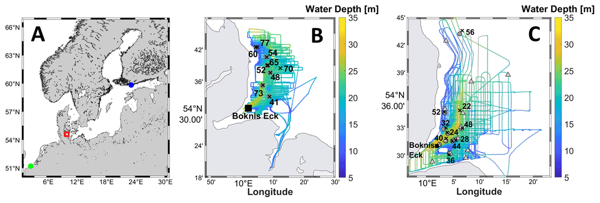
Figure 1(a) Overview map of the Baltic Sea and the southeastern North Sea. The red square marks the research area of this study in the Kiel Bight. The green and blue circles mark the sampling sites of Borges et al. (2019) and Humborg et al. (2019), respectively. (b) Cruise track of cruise AL510 in June 2018. (c) Cruise track of cruise AL516 in September 2018. The black crosses mark CTD stations, dark grey dots mark zodiac sampling sites, and light grey triangles mark UW sampling sites. The maps were computed using the m_map toolbox in MATLAB (Pawlowicz, 2020).
To examine potential CH4 concentration gradients in the very near-surface waters, additional samples from a zodiac were taken at selected stations. To avoid turbulence distributions caused by the ship, the seawater samples were taken at some distance from the ship. Using a self-built sampling device that consisted of an aquarium pump attached to a floating board, water from 0.1, 0.5, and 1 m depth below the surface was pumped on board the zodiac as described in detail by Fischer et al. (2019). In addition, discrete underway (UW) samples were taken from the ship's continuous seawater supply system with a water inlet at ∼ 2 m depth.
Triplicate water samples were taken through a silicon hose connected to the Niskin bottle (CTD samples), aquarium pump (zodiac samples), or the ship's underway system (UW samples). At a low flow rate, 20 mL amber glass vials were filled bubble-free by overflowing with an approximate threefold volume of seawater. The vials were closed with butyl rubber stoppers and crimp-sealed with aluminium caps. To inhibit microbial activity, 50 µL of saturated mercury chloride solution (HgCl2 (aq)) was added to each sample. To compensate for the added volume of HgCl2 solution, a needle with a 3 mL syringe body was inserted into each sample before HgCl2 injection. The samples were stored at room temperature in the dark until the measurements were carried out.
2.1 Purge and trap system
We used a self-built purge and trap (PT) system coupled to a gas chromatograph equipped with a flame ionization detector (GC-FID) to measure CH4 in the surface water and the water column. The set-up (Fig. 2) of the PT measurement system (Fig. 2a) can be divided into three sections that describe the purge unit (Fig. 2b), the trapping unit (Fig. 2c), and the GC-FID system (Fig. 2d). The materials that were used and all performance tests that were carried out are described in detail elsewhere (Gindorf, 2020). Helium (He) is used as the purge gas and as the carrier gas for the GC. The gas stream is split and directed through the purge unit, while a continuous gas stream through the GC is maintained. A digital thermometer is installed next to the system to monitor the temperature.

Figure 2Schematic illustration of the PT system set-up: (a) general set-up of the PT system, the components of the purge unit, the trapping unit, and the GC-FID are shown in detail in (a)–(c); (b) set-up of the purge unit showing the direction of the He gas stream when samples are purged (red) and when the purge chamber is emptied (blue); (c) set-up of the trapping unit showing the direction of the He gas stream when the gas is trapped (red) and desorbed (blue); (d) set-up of the GC-FID system. The individual components of the PT system are (1) He gas cylinder with pressure regulator, (2) sample vial, (3) needle valve, (4) four-port valve, (5) thermometer, (6) double-walled wastewater pipe and wastewater canister, (7) purge chamber, (8) Luer-Lock injection port with check valve and Safeflow® infusion valve, (9) compressed air cylinder with pressure regulator, (10) filter, (11) Nafion® counterflow drying tube, (12) two glass dry traps filled with P2O5, (13) flowmeter, (14) VICI Valco® six-port valve, (15) Dewar tank filled with liquid nitrogen, (16) CH4 trap filled with molecular sieve (5 Å), (17) water boiler, (18) vent, and (19) connection to GC-FID.
The purge unit contains a two-position four-port valve that can be switched to enable the purging of the sample (“purge” mode) or the emptying of the purge chamber (“waste” mode). In the purge mode, the He gas stream is directed through the sample vial and consecutively through the purge chamber. The sample water is pushed into the purge chamber when the He gas stream is turned on. A long needle that reaches the bottom of the sample vial is used to completely empty the vial. Backflushing of the water into the sample vial is restricted by two check valves at the hose between the purge chamber and the sample. The purge chamber consists of a 50 mL sample vial that is placed upside down to minimize leakage through the stopper. The purge flow is directed into the purge chamber through a short needle with the needle tip placed close to the stopper to ensure the purging of the entire water sample. When the He gas is bubbling through the sample, the dissolved gases are stripped from the water phase. Due to its low solubility in seawater at room temperature and normal pressure (Duan et al., 1992), CH4 is stripped out within 4 min using a purge flow of approximately 0.03 L min−1. The gas is extracted from the purge chamber via a long needle with the needle tip placed close to the bottom of the upside-down vial. The gas is then dried over a Nafion™ dryer with a counterflow of dry compressed air at a flow rate of approximately 200 mL min1. Additionally, two glass tubes filled with phosphorus pentoxide (Sicapent®; P2O5) are used to further dry the gas stream. To ensure a continuous and uniform flow rate during the measurements, a flowmeter is installed before the gas is transferred to the trapping unit.
The He gas stream from the purge unit and the carrier gas stream of the GC are connected to a two-position six-port valve that enables the switching of the gas stream through the CH4 trap. In the “trap” position, the purge gas is conducted through the trap, which consists of a 20 cm × in. (0.3175 cm diameter) stainless steel column filled with Spherocarb (100–200 mesh). The trap is put into liquid nitrogen during the trapping procedure. In the “desorb” position, the GC carrier gas flow is conducted through the trap, which is subsequently removed from the liquid nitrogen and put into a water bath of ∼ 90 ∘C to desorb the trapped gases from the column. The gas flow is then directed through the GC-FID system.
The GC-FID used in this set-up is an HP 5890 II GC equipped with an FID detector. The gases are separated over a 6 ft × in. (182.88 cm long, 0.3175 cm diameter) stainless steel column, with a carrier gas flow of ∼ 30 mL min−1. A similar flow rate of the carrier gas streams during the trapping and the desorption steps was chosen to avoid baseline shifts when switching the Valco valve.
2.2 Calibration
On each measurement day, a set of standard gas mixtures and blank measurements with and without the injection of 20 mL He was measured prior to sample measurements. The gas standards have been calibrated against two National Oceanic and Atmospheric Administration (NOAA) primary standards that were provided by the SCOR Working Group 143 for the intercomparison of oceanic CH4 and N2O measurements (Wilson et al., 2018). Prior to standard measurements, one seawater sample was purged on every measurement day. This water was left inside the purge chamber and used for the blank and standard measurements. For the standard and He blank injection, 20 mL plastic syringes were used. A Safeflow® infusion valve was attached to the check valve at the standard injection port to reduce the dead volume of the injection port. After each standard injection, 3 mL of He was injected with a 3 mL plastic syringe through the port to ensure that all the injected volume of the standard is injected into the purge chamber. The He flow through the purge unit is switched off during the standard injection. Different volumes of the standard were injected into the purge system to create a calibration curve that covered the full concentration range of the samples. The amount of the injected standards was calculated from the respective mole fraction and the injected volume using the ideal gas law. The chromatography software ChromStar 6.3 (SCPA GmbH, Weyhe-Leeste, Germany) was used for data acquisition and manual integration of the CH4 peaks.

Figure 3Boknis Eck depth profile of CH4 measured with PT (light grey) and HS (dark grey) in April 2020 (a). Means are shown as filled dots and the dashed line, and standard deviation is displayed as error bars in the respective colours. Linear regression of CH4 concentrations measured with PT against HS for samples from Boknis Eck in April 2020 (b). The light grey dashed line indicates the 1:1 relation. y = . R2 = 0.999; p<0.0001.
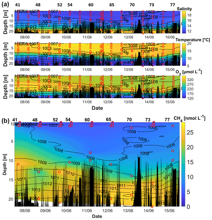
Figure 4(a) Salinity (upper sub-panel), temperature (middle sub-panel), and O2 (lower sub-panel) during AL510 in June 2018. (b) CH4 concentrations during AL510. Red circles mark the location of the discrete measurements. Black peaks show the topography along the cruise track. Contour lines represent the density. Data for CH4 were not available for the beginning of the cruise because the measurements started on 7 June 2018. The station numbers in (b) refer to those in Fig. 1.
2.3 Comparison of static headspace equilibrium and purge and trap
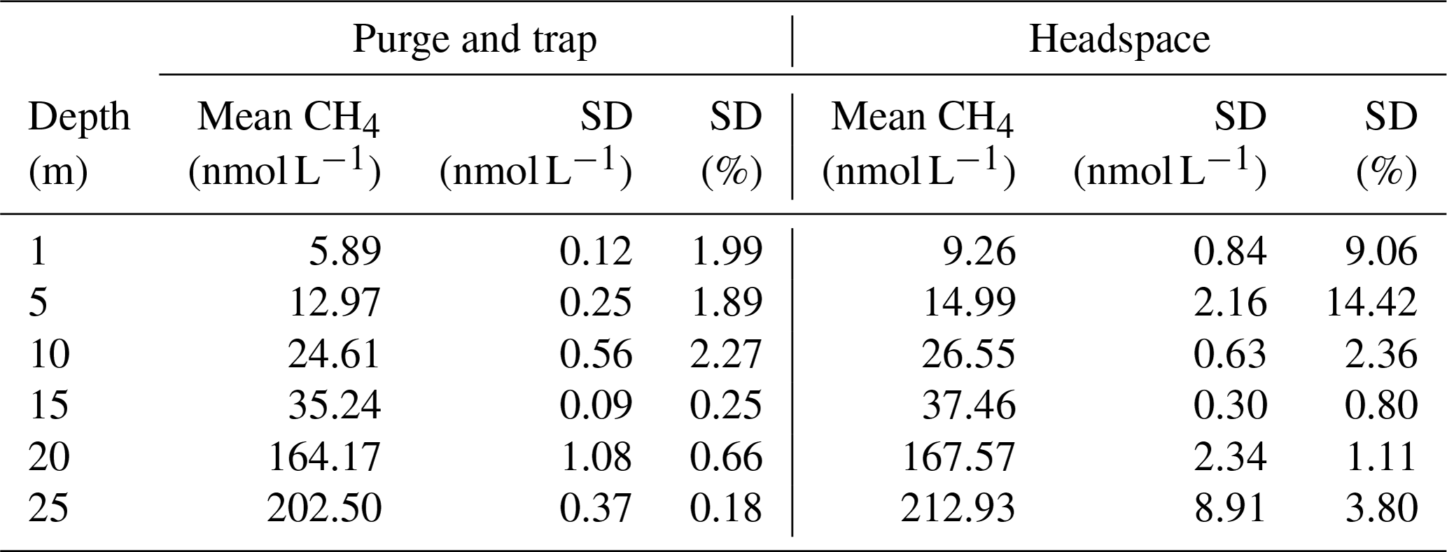
To ensure that the PT measurements are comparable to measurements with the previously used static headspace equilibration (HS) method (see, for example, Ma et al., 2020), triplicates of seawater samples from the six standard depths were taken for PT and HS during a Boknis Eck cruise. The CH4 concentrations ranged from 5 to 222 nmol L−1, allowing a comparison over a broad concentration range (Fig. 3). Over all depths, the PT-measured concentrations were slightly lower and showed significantly less variation among the triplicates, thereby reflecting a better precision of the PT measurements over the HS method (Table 1). The direct comparison of both techniques shows that the measurements agree well with the HS measurements (Fig. 4). Other studies have proven higher precision and sensitivity, as well as handling benefits, of PT over HS (e.g. Capelle et al., 2015).
Table 1Boknis Eck April 2020 concentrations and deviations measured with PT and HS.
2.4 Calculation of dissolved CH4 concentrations
The CH4 concentration in the sample was calculated from the linear calibration fit using Eq. (1). The mean area of the blank measurements was subtracted from the sample peak area to account for the background contamination of the system.
where n is the amount of CH4 [nmol] in the sample, PASample is the peak area of the measured sample, PABlank is the mean peak area of the measured blanks, and δ is the slope of the calibration curve [nmol−1].
The CH4 concentration c [nmol L−1] was calculated as the ratio between n and the sample volume V [L]. V was determined experimentally to be 0.0203 ± 0.0002 L.
We estimated the standard deviation (SD) for triplicates or duplicates according to the statistical analysis of David (1951). The mean analytical error of the CH4 concentration was ± 5.7 % and 3.1 % during the June and September cruises, respectively.
2.5 ΔCH4 and CH4 saturations
Temperature and salinity data from the ship's thermosalinograph were used to compute the excess of CH4 (ΔCH4) as the difference between the measured CH4 concentration (c, see above) and the CH4 equilibrium concentration (ceq). The solubility equation for CH4 in seawater (Wiesenburg and Guinasso, 1979) was applied to calculate ceq (in nmol L−1). The atmospheric dry mole fraction of CH4 was taken from records of the Mace Head observatory in Ireland (Dlugokencky, 2020). The monthly means of atmospheric CH4 were 1918.24 ppb ± 0.2 % for June and 1925.83 ppb ± 0.2 % for September 2018.
CH4 saturations (CH4sat in %) were computed as
2.6 Oxygen measurements
During both cruises, a CTD-mounted altimeter (sn#453) oxygen sensor was used to obtain CTD O2 profiles from the surface to 1 m above the bottom. Additionally, 112 and 105 discrete oxygen samples were Winkler titrated during the June and September cruises, respectively, and were used to calibrate the sensor data.
2.7 Temperature and CH4 anomalies
The measurements at the Boknis Eck Time Series Station performed during this study allows us determine the effect of the European heatwave in 2018 in the context of the monthly time-series measurements of water temperature and dissolved CH4 at Boknis Eck (Lennartz et al., 2014; Ma et al. 2020). To this end, we computed the anomalies of water temperature and ΔCH4 at 1 and 25 m water depth for the period of January 2006 to December 2018. The anomalies were defined as
and
where T is the measured monthly water temperature in the period January 2006 to December 2018 at 1 and 25 m depth at Boknis Eck (Lennartz et al., 2014). Ti, avg is the mean water temperature at 1 and 25 m depth of the respective month i over this period at Boknis Eck. The resulting ΔT is the anomaly of the water temperature which is cleaned from seasonal differences throughout each year. Δ (ΔCH4) is calculated similarly to ΔT in the same time period using ΔCH4, which is the monthly excess CH4 (ΔCH4, see above) at 1 and 25 m depth. (ΔCH4)i, avg is the mean excess CH4 at 1 and 25 m depth of the respective month i over this period at Boknis Eck. ΔCH4 was computed as the difference of the monthly measurements of dissolved CH4 at 1 and 25 m water depth (Ma et al., 2020) and the monthly ceq (see Sect. 2.5) at 1 and 25 m water depth. ceq was calculated with the monthly water temperature and salinity at Boknis Eck at 1 and 25 m depth (Lennartz et al., 2014) and the monthly atmospheric CH4 dry mole fractions measured at Mace Head (see Sect. 2.5) from January 2006 to December 2018. Extremely high CH4 surface concentrations with concentrations in the range from 87 to 689 nmol L−1 have been measured in 4 months (November 2013, February/March 2014, and December 2014) and were, thus, omitted from the data set to avoid a statistical bias of the data set.
3.1 June 2018
The hydrographic conditions during the June cruise revealed a strong stratification of the water column: while the upper ∼ 10 m were comparably uniform, a strong gradient in temperature prevailed between 10 and 15 m, and the lower water column (15–20 m) showed a strong salinity gradient (Fig. 4). This is in line with former studies in the respective area (e.g. Bange et al., 2010; Dale et al., 2011; Lennartz et al., 2014; Ma et al., 2019, 2020).
Between 9 and 13 June, surface water temperatures exceeded 20 ∘C, which is higher than the average surface temperature measured at the Boknis Eck station in June (Lennartz et al., 2014).
The highest O2 concentrations were measured between approximately 7 and 18 m depth and between the 1009 and the 1012 kg m−3 isopycnals. At the beginning of the measurements, the O2 maximum had a vertical extension of more than 10 m, which decreased continuously in its thickness and intensity until it vanished after 15 June. The whole water column was oxygenated throughout the cruise, with oxygen concentrations decreasing to ∼ 120 µmol L−1 in the bottom waters. At this time of the year, the oxygen depletion in the deep water starts to evolve (Lennartz et al., 2014). The water column CH4 concentrations ranged from 2.8 nmol L−1 (99 % saturation) in the surface waters to 28.3 nmol L−1 (750 %) in the bottom waters.
3.2 September 2018
During the September campaign, the water column also showed a strong stratification below 10 m with pronounced gradients in temperature, salinity, and O2 concentrations (Fig. 5). In contrast to the cruise in June, the stratification below 10 m seemed to be primarily driven by the salinity gradient. The surface water showed a comparably homogeneous distribution of about 17 ∘C down to the 1014 kg m−3 isopycnal at ∼ 15 m. A strong temperature decrease was observed below 20 m, with temperatures ∼ 12 ∘C in the bottom waters. An increased surface density at the beginning and the end of the cruise (before 14 September, after 22 September) indicated the upwelling of waters from 5–10 m to the surface. A strong storm event on the 21st could have induced this upwelling (mean wind speed on the 21st ∼ 12 m s−1). The bottom-water salinity was lower at the beginning than at the end of the cruise, and the higher salinities were shifted upward in the water column in agreement with the upshift of the 1016 kg m−3 isopycnal.
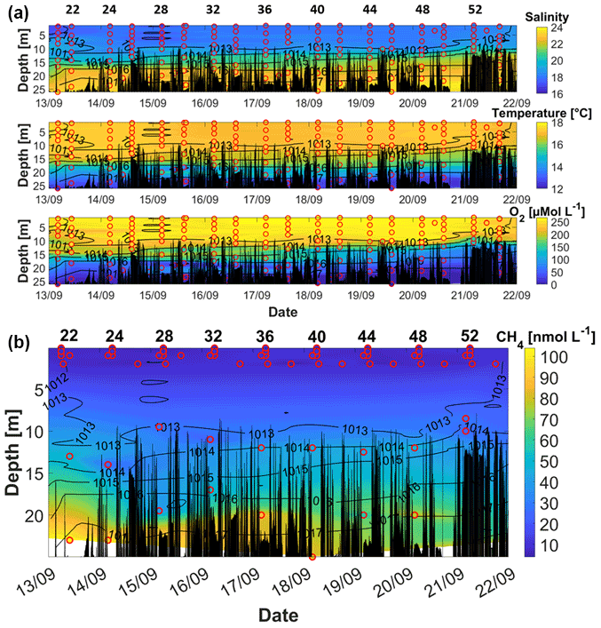
Figure 5(a) Salinity (upper sub-panel), temperature (middle sub-panel), and O2 (lower sub-panel) during September 2018. (b) CH4 concentrations in September. Red circles mark the location of the discrete measurements. Black peaks show the topography along the cruise track. Contour lines represent the density. The station numbers refer to those in figure 1.
During the whole cruise, the highest O2 concentrations were measured in the surface waters above the 1013 kg m−3 isopycnal. Between the 1014 and 1015 kg m−3 isopycnals a strong oxycline could be observed as O2 decreased by approximately 100 µmol L−1 within a few metres. With increasing depth, the O2 concentration decreased to suboxic (O2 < 5 µmol L−1) and almost anoxic (O2 ∼ 0 µmol L−1) conditions in the bottom water. However, during the September cruise no indication of sulfidic conditions (e.g. the smell of hydrogen sulfide) was observed. Along with the upward-shifting isopycnals, hypoxia (O2 < 60 µmol L−1) characterized almost half of the water column at the end of the cruise. Intense hypoxic and even anoxic conditions in the bottom water have been frequently observed at the Boknis Eck Time Series Station (Eckernförde Bay) between late summer and autumn (e.g. Bange et al., 2010; Dale et al., 2011; Lennartz et al., 2014; Ma et al., 2019, 2020).
CH4 concentrations ranged from 4.7 nmol L−1 at the surface to 104.0 nmol L−1 in the bottom waters (Fig. 5b). In contrast to the O2, temperature, and salinity profiles, the CH4 distribution in the bottom and intermediate waters showed a larger variability. The strongest accumulation of CH4 was confined to the bottom waters below 20 m. Although the surface samples revealed a stronger oversaturation of CH4 than during the June campaign (see Fig. 6), the stratification of the water column seemed to be an effective barrier for the CH4 from the bottom waters reaching the atmosphere.
3.3 CH4 in the surface layer
During both cruises, the surface layer was always oversaturated or close to equilibrium with the atmosphere (Fig. 6). ΔCH4 ranged between ∼ 0 and 6 nmol L−1 during the June cruise and between 2 and 8 nmol L−1 during the September cruise, corresponding to saturations of 103 %–292 % and 201 %–366 %, respectively. The near-surface samples of CH4 from the zodiac and underway measurements revealed that within the top 1 m of the water column, CH4 concentration gradients existed (see Fig. 7), with larger concentration differences between 0.1 and 1 m (0.2–2.7 nmol L−1) than between 1 and 2 m (0.1–1.8 nmol L−1; mean difference between CH4 gradients: ∼ 1 nmol L−1) during the September cruise. The direction of the gradients was highly variable, with some stations showing higher CH4 concentrations in the topmost sample, while others displayed increasing concentrations with depth or intermediate maxima.
Interestingly, the CH4 concentrations measured from the shallowest Niskin bottles (1–2 m) were generally higher than from the surface samples (average difference between CH4 concentrations from Niskin bottle and from zodiac samples: 1.2 ± 0.4 nmol L−1). This could reflect the different sampling conditions, but it may also be a sign of mixing or carry-over effects from the CTD profiling. This can result from closing the Niskin bottles during the upcast so that deeper waters might be brought up. A comparably large variation between the triplicate samples may result from the challenging sampling conditions on board of the zodiac. However, the majority of the observed gradients are larger than the cumulative uncertainty of the replicate measurements.
The sampling depth for surface water is not uniformly defined in oceanic measurements. While for the open ocean, CTD sampling depths down to 10 m are recognized as surface samples, for coastal areas often 1 m is considered as the surface depth (e.g. Ma et al., 2020). For continuous UW measurements the sampling depth depends on the vessel's hull and water intake depth which can range between 1 and 10 m depth (e.g. 2–5 m; Becker, 2016; Karlson et al., 2016; Kitidis et al., 2010; Rhee et al., 2009; Zhang et al., 2014). Although the near-surface gradients found in our study do not show a clear direction, our results indicate that at least in coastal areas with elevated CH4 concentrations, a sampling depth of several metres may not correctly represent the surface CH4 concentration.
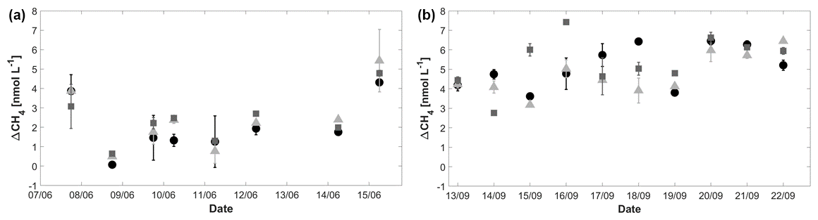
Figure 6ΔCH4 in June (a) and September (b) for surface water at 0.1 m depth (dots), 0.5 m depth (triangles), and 1 m depth (squares). Error bars were calculated as described in the Methods section.
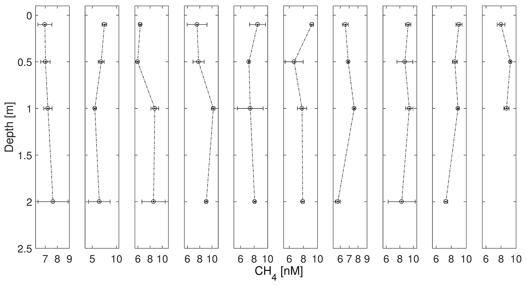
Figure 7Near-surface profiles of CH4 with sampling from the zodiac and UW sampling from the ship (∼ 2 m) during AL 516 in September 2018. The time lag between zodiac sampling and UW sampling was max 1 h. All samplings were conducted in the morning (∼ 06:00 local time). Error bars indicate 95 % confidence interval (CI), calculated from triplicate measurements.
3.4 Seasonal variability
Please note that when comparing June and September data from Figs. 4 and 5, different colour schemes were used to emphasize gradients within each cruise. Between June and September, a strong increase in the salinity, along with changes in the vertical temperature distribution, indicated an exchange of the waters in the western Kiel Bight over the entire water column (Fig. 8). With the change in the water masses, a clear shift in the CH4–O2 relationship from June to September was observed (Fig. 9). While only a slight increase in the surface CH4 concentrations was observed between June and September, much higher bottom CH4 concentrations and much lower O2 concentrations were found in September. The co-occurrence of O2 depletion and CH4 enrichment in the bottom water agrees with the observations from previous studies (e.g. Bange et al., 2010; Steinle et al., 2017).
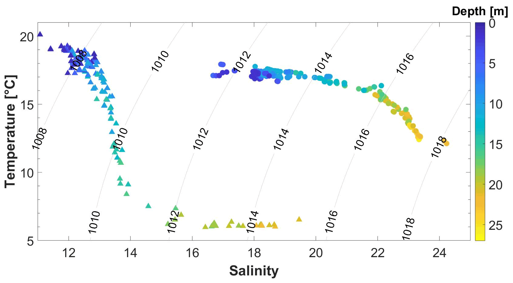
Figure 8Temperature and salinity diagram of CTD bottle data from June 2018 (triangles) and September 2018 (circles). Grey lines represent the corresponding isopycnals (in kg m−3).
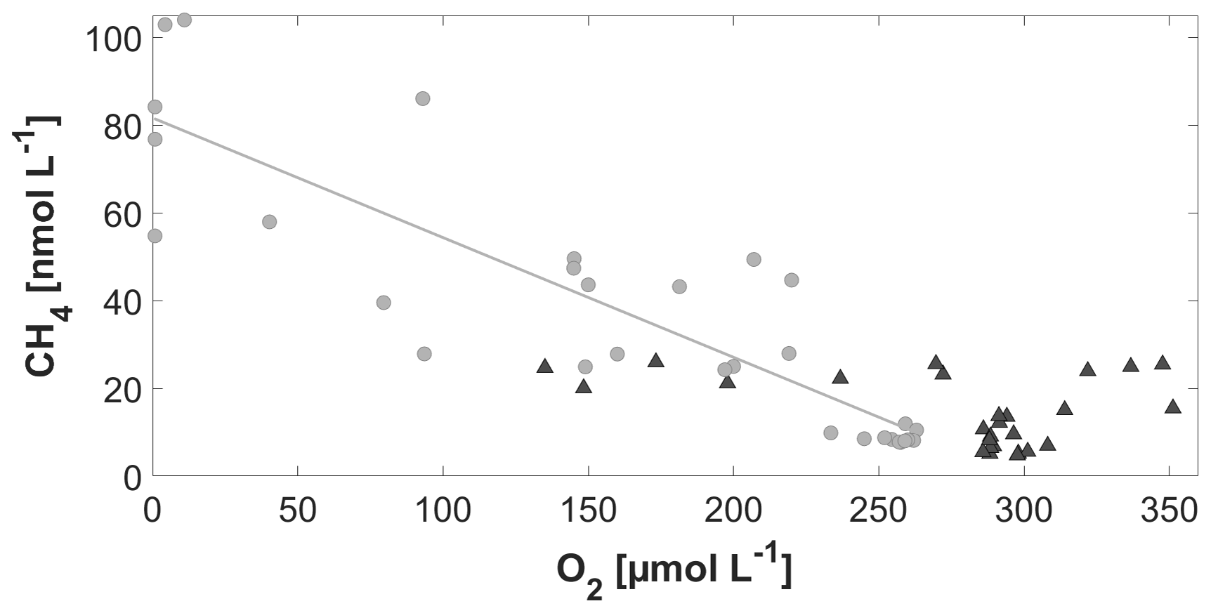
Figure 9Comparison of the relationship of CH4 vs. O2 in June (black triangles; p=0.07) and September (filled grey circles; ; R2 = 0.764; p=<0.0001).
The high CH4 concentration in the bottom water most likely results from methanogenesis in the anoxic sediments (Bange et al., 2010) producing CH4 that is partly released into the water column (Donis et al., 2017; Reindl and Bolałek, 2014). The summer stratification inhibits the CH4 from reaching the surface, and, thus, CH4 accumulates below the pycnocline. Within the water column, CH4 is efficiently oxidized, and only a small fraction reaches the surface layer (Steinle et al., 2017). The salinity change between June and September also indicates that the high CH4 concentration in the bottom water in September does not result from long-term accumulation of CH4 in the bottom waters. It is rather the result of recent local CH4 release either at the BE site itself or advected to the BE site by the bottom waters.
3.5 The 2018 European heatwave impact on CH4
Figure 10 shows the anomalies of T and ΔCH4 at 1 and 25 m water depth from January 2006 to December 2018. A pronounced temperature anomaly is visible at 1 m depth in August 2018 reflecting the heatwave which occurred from mid-July to August 2018 across northwestern Europe (Kueh and Lin, 2020). However, a signal of the 2018 heatwave is not visible in the temperature anomalies at 25 m depth. The maximum anomaly of ΔCH4 at 1 m water depth is visible in May 2018 and thus not associated with the heatwave signal of the temperature anomaly at 1 m. The maximum temperature anomaly is found at 1 m water depth for July 2006 and reflects another European heatwave which was experienced by large parts of western and central Europe during July 2006 (Chiriaco et al., 2014). Again, the signal of the 2006 heatwave is not visible in the anomalies of ΔCH4. Overall, there is no relationship between the water temperature anomalies and ΔCH4 anomalies at both 1 and 25 m depths.
This finding is in contrast to the results by Borges et al. (2019), who reported significantly enhanced CH4 surface concentrations in coastal waters of the North Sea off Belgium in July 2018 (Fig. 1). They hypothesized that the high dissolved CH4 surface concentrations might have been caused by a temperature-driven enhancement of both methanogenesis and sedimentary release of CH4. Humborg et al. (2019) measured dissolved CH4 surface concentrations in the coastal waters of southern Finland after the heatwave in September 2018 (Fig. 1). They concluded that the heatwave caused higher CH4 emissions to the atmosphere from near-shore sites which, in turn, might have been fuelled by temperature-driven sedimentary release of CH4. However, our data do not support a heatwave-driven enhancement of CH4 concentrations at Boknis Eck (Eckernförde Bay) (see Fig. 10). Thus, CH4 emissions to the atmosphere at Boknis Eck do not seem to be affected by the heatwaves.
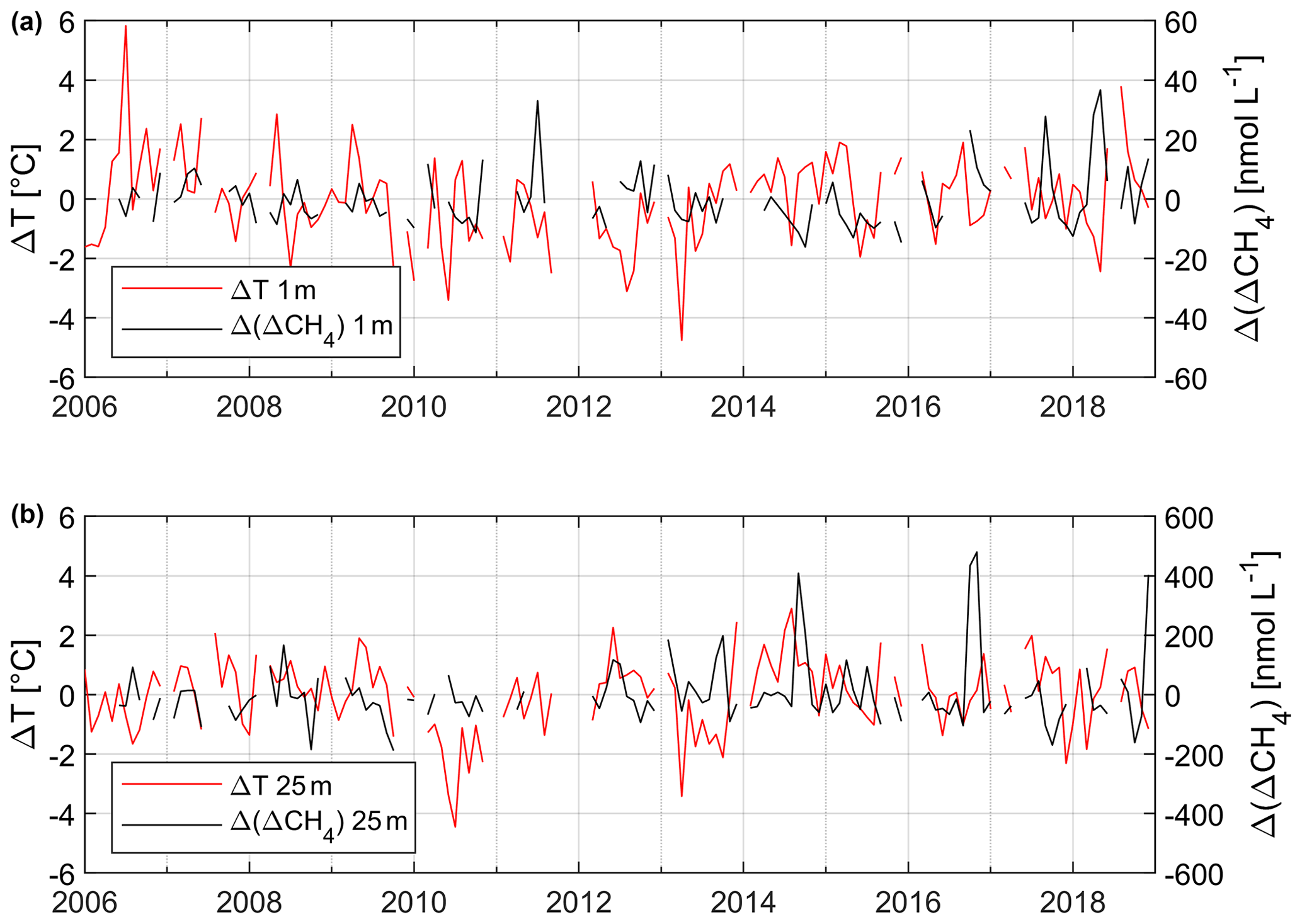
Figure 10Monthly anomalies of temperature (ΔT, solid red line, left y axis) and ΔCH4 (Δ (ΔCH4), solid black line, right y axis) at 1 (a) and 25 m (b) from 2006 to 2019. Please note that gaps in the data sets are caused by missing data.
The shallow coastal waters off the Belgian coast (water depth <30 m) are characterized by strong tidal currents which result in a well-mixed water column throughout the year (Borges et al., 2019). This implies that the temperature signal of the 2018 heatwave was most likely conveyed to the sediments and might have led to enhanced release of CH4 due to enhanced methanogenesis in combination with ebullition of CH4 from CH4-enriched (gassy) sediments (Borges et al., 2019). In contrast, the water column at Boknis Eck was stratified during summer 2018. Therefore, the temperature signal of the heatwave was only detectable in the surface layer but not in the bottom layer, and a potential heatwave-triggered CH4 release from the sediments was not detected (Fig. 10).
In contrast to the measurements at Boknis Eck, the shallow bottom waters (water depth = 31 m) at the Tvärminne Zoological Station (TZS) coastal monitoring station (northeastern Baltic Proper) showed a significant temperature signal in 2018 (Humborg et al., 2019). The enhanced bottom-water temperatures, in turn, might have led to an enhanced outgassing of sedimentary CH4 via gas plumes (Humborg et al., 2019).
On the one hand, a temperature increase should lead to enhanced microbial CH4 production, but, on the other hand, its microbial consumption by aerobic and anaerobic CH4 oxidation should increase as well in both the water column and the sediments. At Boknis Eck, for example, methanogenesis and CH4 oxidation indeed show the same seasonal (i.e. temperature) dependencies (Maltby et al., 2018; Steinle et al., 2017; Treude et al., 2005). This implies that a temperature increase most probably results only in a small increase in the net CH4 production (= methanogenesis minus CH4 oxidation). Any significantly enhanced CH4 concentrations resulting from an increase in temperature might be, therefore, dominated by enhanced ebullition from gassy sediments in shallow coastal waters which are (i) well-mixed (as observed off the Belgian coast; Borges et al., 2019) or which (ii) show a deepening of the mixed layer to allow gas plumes to reach the mixed layer (as observed off southern Finland; Humborg et al., 2019). Despite the fact that CH4-enriched (gassy) sediments are also found in Eckernförde Bay (Lohrberg et al., 2020), the prerequisites (bottom-water temperature anomaly and ebullition) for a heatwave-induced enhancement of CH4 surface concentrations have not been observed at Boknis Eck during our study in 2006 and 2018. Boknis Eck experienced heatwaves after 2018. However, CH4 concentration measurements from Boknis Eck after 2018 were not available at the time of the writing of this article.
The frequency of higher ΔCH4 anomalies at 25 m seems to have increased since 2013 (Fig. 10). We may, thus, speculate that sedimentary release of CH4 to the overlying water column may have increased as well, which in turn might be caused by the long-term warming trend observed at Boknis Eck (Lennartz et al., 2014).
Our measurements revealed higher CH4 concentrations in the bottom waters and comparably lower CH4 concentrations in the surface waters which were caused by a stratification of the water column. This, in turn, prevented upward mixing of CH4-enriched waters during both campaigns. CH4 concentrations in the bottom waters were significantly higher in September compared to June and were accompanied by a strong decrease in O2 concentrations in the bottom water which led to anoxic conditions favourable for microbial CH4 production in September 2018. The overall setting of the CH4 water column distribution and the comparably rapid seasonal change in the CH4 concentrations is in line with the time-series measurements of dissolved CH4 concentrations at the Boknis Eck Time Series Station in Eckernförde Bay (Ma et al., 2020; Maltby et al., 2018; Steinle et al., 2017).
In summer 2018, northwestern Europe was experiencing a pronounced heatwave which led to significantly enhanced water temperatures in the Baltic and the North seas. This, in turn, might have triggered enhanced CH4 production and consequently might have led to enhanced CH4 concentrations (Borges et al., 2019; Humborg et al., 2019). However, we found no relationship between the anomalies of water temperature and excess CH4 in both the surface and the bottom layers at Boknis Eck (Eckernförde Bay) for the period 2006 to 2018. We conclude that pronounced European heatwaves which, for example, occurred in 2006 and 2018 did not affect CH4 concentrations in the Eckernförde Bay. Therefore, the 2018 European heatwave most likely had no effect on the observed increase in the CH4 concentrations in the western Kiel Bight from June to September 2018.
CH4 saturations in the surface layer were always >100 %, and, thus, the western Kiel Bight and Eckernförde Bay were sources of CH4 to the atmosphere during both June and September 2018. This agrees with the fact that the Baltic Sea is a source of atmospheric CH4 throughout the year (see, for example, Gülzow et al., 2013; Gutiérrez-Loza et al., 2019; Ma et al., 2020). The high-resolution measurements of the CH4 concentrations in the upper 1 m of the water column were highly variable and showed no uniform decreasing or increasing gradients with water depth. Surface CH4 concentration measurements used for flux calculations are usually from one depth in the surface layer assuming that there are no concentration gradients and that the CH4 concentration in the surface layer is uniform. Our results imply that the assumption of a uniform distribution of CH4 concentrations in the upper surface layer is not justified. Thus, CH4 flux calculations on the basis of the concentration difference across the ocean–atmosphere interface is associated with a degree of uncertainty when ignoring the CH4 variability in the upper surface layer (Fischer et al., 2019; Calleja et al., 2013). However, since there were no uniform increasing or decreasing CH4 gradients, we cannot assess whether CH4 flux calculations would have been generally under- or overestimated.
Overall, our results show that the CH4 distribution in the water column of the western Kiel Bight and Eckernförde Bay is strongly affected by both large-scale (i.e. seasonal) and small-scale variabilities. In order to reduce the uncertainties associated with concentration-difference-based CH4 emission estimates, we suggest high-resolution measurements in the upper surface layer on a regular (at least seasonal) basis. This is also in line with a study by Roth et al. (2022) that recently showed that a high sampling frequency of at least 50 samples per day is needed to resolve the high variability in CH4 emissions from coastal habitats. This emphasizes the need of a higher resolution of the CH4 dynamics in coastal environments for future studies.
The data are available from the PANGAEA database (Gindorf et al., 2020a, b) for AL510 (June) and AL516 (September), respectively. Data from the Boknis Eck Time Series Station are available from the Boknis Eck database at https://www.bokniseck.de//database-access (Bange and Malien, 2022). All data will be available from the MEMENTO (MarinE MethanE and NiTrous Oxide) database at https://memento.geomar.de (Kock and Bange, 2015).
AK, DB, and HWB designed the study. SG set up the purge and trap system and performed the measurements. AK, HWB, and SG wrote the manuscript. DB carried out the sampling during both campaigns and contributed to the manuscript.
The contact author has declared that none of the authors has any competing interests.
Publisher’s note: Copernicus Publications remains neutral with regard to jurisdictional claims in published maps and institutional affiliations.
We thank the captain and crew of R/V Alkor for their support during the Baltic GasEx cruises. We would like to thank Melf Paulsen, Hanna Campen, and Riel Carlo Ingeniero for their support with the laboratory equipment, as well as Tina Fiedler for the laboratory maintenance and Xiao Ma for his help with the data acquisition. We especially thank Tim Fischer for the deployment of the gradient pump system during the zodiac trips. This work was part of the BONUS INTEGRAL project which received funding from BONUS (Art 185), funded jointly by the EU, the German Federal Ministry of Education and Research, the Swedish Research Council Formas, the Academy of Finland, the Polish National Centre for Research and Development, and the Estonian Research Council. The Baltic GasEx project was supported by GEOMAR. The Boknis Eck Time Series Station is an endorsed project of the international Surface Ocean–Lower Atmosphere Study (SOLAS: https://www.solas-int.org, last access: 21 October 2022) and Baltic Earth (https://www.baltic.earth, last access: 21 October 2022).
This research has been supported by the European Commission, Horizon 2020 (BONUS (grant no. 271534)).
The article processing charges for this open-access publication were covered by the GEOMAR Helmholtz Centre for Ocean Research Kiel.
This paper was edited by Helge Niemann and reviewed by Oliver Schmale and one anonymous referee.
Bakker, D. C. E., Bange, H. W., Gruber, N., Johannessen, T., Upstill-Goddard, R. C., Borges, A. V., Delille, B., Löscher, C. R., Naqvi, S. W. A., Omar, A. M., and Santana-Casiano, J. M.: Air-sea interactions of natural long-lived greenhouse gases (CO2, N2O, CH4) in a changing climate, in: Ocean-Atmosphere Interactions of Gases and Particles, edited by: Liss, P. S. and Johnson, M. T., Springer, Heidelberg, Germany, 113–169, https://doi.org/10.1007/978-3-642-25643-1, 2014.
Bange, H. W. and Malien, F.: Boknis Eck Time-series Database, Kiel Datamanagement Team [data set], https://www.bokniseck.de//database-access, last access: 21 October 2022.
Bange, H. W., Bergmann, K., Hansen, H. P., Kock, A., Koppe, R., Malien, F., and Ostrau, C.: Dissolved methane during hypoxic events at the Boknis Eck time series station (Eckernförde Bay, SW Baltic Sea), Biogeosciences, 7, 1279–1284, https://doi.org/10.5194/bg-7-1279-2010, 2010.
Bange, H. W., Hansen, H. P., Malien, F., Laß, K., Karstensen, J., Petereit, C., Friedrichs, G., and Dale, A.: Boknis Eck Time Series Station (SW Baltic Sea): Measurements from 1957 to 2010, LOICZ-Affiliated Act., Inprint, 20, 16–22, 2011.
Becker, M.: Autonomous 13C measurements in the North Atlantic – a novel approach for identifying patterns and driving factors of the upper ocean carbon cycle. Open Access (PhD/ Doctoral thesis), Christian-Albrechts-Universität Kiel, Kiel, Germany, 151 pp., 2016.
Booge, D.: Cruise Report AL510, 1–23, https://doi.org/10.3289/CR_AL510, 2018a.
Booge, D.: Cruise Report AL516, 1–25, https://doi.org/10.3289/CR_AL516, 2018b.
Borges, A. V., Royer, C., Martin, J. L., Champenois, W., and Gypens, N.: Response of marine methane dissolved concentrations and emissions in the Southern North Sea to the European 2018 heatwave, Cont. Shelf Res., 190, 104004, https://doi.org/10.1016/j.csr.2019.104004, 2019.
Calleja, M. L., Duarte, C. M., Álvarez, M., Vaquer-Sunyer, R., Agustí, S., and Herndl, G. J.: Prevalence of strong vertical CO2 and O2 variability in the top meters of the ocean, Global Biogeochem. Cy., 27, 941–949, https://doi.org/10.1002/gbc.20081, 2013.
Capelle, D. W., Dacey, J. W., and Tortell, P. D.: An automated, high through-put method for accurate and precise measurements of dissolved nitrous-oxide and methane concentrations in natural waters, Limnol. Oceanogr. Method., 13, 345–355, https://doi.org/10.1002/lom3.10029, 2015.
Chiriaco, M., Bastin, S., Yiou, P., Haeffelin, M., Dupont, J. C., and Stéfanon, M.: European heatwave in July 2006: Observations and modeling showing how local processes amplify conducive large-scale conditions, Geophys. Res. Lett., 41, 5644–5652, https://doi.org/10.1002/2014GL060205, 2014.
Dale, A. W., Sommer, S., Bohlen, L., Treude, T., Bertics, V. J., Bange, H. W., Pfannkuche, O., Schorp, T., Mattsdotter, M., and Wallmann, K.: Rates and regulation of nitrogen cycling in seasonally hypoxic sediments during winter (Boknis Eck, SW Baltic Sea): Sensitivity to environmental variables, Estuar. Coast. Shelf Sci., 95, 14–28, https://doi.org/10.1016/j.ecss.2011.05.016, 2011.
David, H. A.: Further Applications of Range to the Analysis of Variance, Oxford Univ. Press behalf Biometrika Trust, 38, 393–409, https://doi.org/10.2307/2332585, 1951.
Dlugokencky, E.: Monthly Averages of CH4 at Mace Head, County Galway, Ireland (MHD), NOAA Earth Syst. Res. Lab. Glob. Monit. Lab., ftp://aftp.cmdl.noaa.gov/data/trace_gases/ch4/flask/surface/ch4_mhd_surface-flask_1_ccgg_month.txt, last access: 6 July 2020.
Donis, D., Janssen, F., Liu, B., Wenzhöfer, F., Dellwig, O., Escher, P., Spitzy, A., and Böttcher, M. E.: Biogeochemical impact of submarine ground water discharge on coastal surface sands of the southern Baltic Sea, Estuar. Coast. Shelf Sci., 189, 131–142, https://doi.org/10.1016/j.ecss.2017.03.003, 2017.
Duan, Z., Møller, N., Greenberg, J., and Weare, J. H.: The prediction of methane solubility in natural waters to high ionic strength from 0 to 250 ∘C and from 0 to 1600 bar, Geochim. Cosmochim. Ac., 56, 1451–1460, https://doi.org/10.1016/0016-7037(92)90215-5, 1992.
Fischer, T., Kock, A., Arévalo-Martínez, D. L., Dengler, M., Brandt, P., and Bange, H. W.: Gas exchange estimates in the Peruvian upwelling regime biased by multi-day near-surface stratification, Biogeosciences, 16, 2307–2328, https://doi.org/10.5194/bg-16-2307-2019, 2019.
Gindorf, S.: Development of a Purge + Trap System for the Quantification of Methane Variability in the Baltic Sea, Open Access (Master thesis), Christian-Albrechts-Universität zu Kiel, Kiel, Germany, 81 pp., 2020.
Gindorf, S., Booge, D., Kock, A., Bange, H. W., and Marandino, C. A.: Surface and water column methane (CH4) distribution and sea-to-air flux during ALKOR cruise AL510, PANGAEA [data set], https://doi.org/10.1594/PANGAEA.923992, 2020a.
Gindorf, S., Booge, D., Kock, A., Bange, H. W., and Marandino, C. A.: Surface and water column methane (CH4) distribution and sea-to-air flux during ALKOR cruise AL516, PANGAEA [data set], https://doi.org/10.1594/PANGAEA.924372, 2020b.
Gülzow, W., Rehder, G., Schneider v. Deimling, J., Seifert, T., and Tóth, Z.: One year of continuous measurements constraining methane emissions from the Baltic Sea to the atmosphere using a ship of opportunity, Biogeosciences, 10, 81–99, https://doi.org/10.5194/bg-10-81-2013, 2013.
Gutiérrez-Loza, L., Wallin, M. B., Sahlée, E., Nilsson, E., Bange, H. W., Kock, A., and Rutgersson, A.: Measurement of air-sea methane fluxes in the baltic sea using the eddy covariance method, Front. Earth Sci., 7, 1–13, https://doi.org/10.3389/feart.2019.00093, 2019.
Ho, D. T., Marandino, C. A., Friedrichs, G., Engel, A., Bange, H., Barthelmess, T., Fischer, T., Koffman, T., Lange, F., Quack, B., Paulsen, M., Schlosser, P., and Zhou, L.: Baltic Sea Gas Exchange Experiment (Baltic GasEx). Open Access [Poster], in: SOLAS Open Science Conference 2019, 21–25 April 2019, Sapporo, Japan, 2019.
Humborg, C., Geibel, M. C., Sun, X., McCrackin, M., Mörth, C. M., Stranne, C., Jakobsson, M., Gustafsson, B., Sokolov, A., Norkko, A., and Norkko, J.: High emissions of carbon dioxide and methane from the coastal Baltic Sea at the end of a summer heat wave, Front. Mar. Sci., 6, 1–14, https://doi.org/10.3389/fmars.2019.00493, 2019.
Karlson, B., Andersson, L. S., Kaitala, S., Kronsell, J., Mohlin, M., Seppälä, J., and Willstrand Wranne, A.: A comparison of FerryBox data vs. monitoring data from research vessels for near surface waters of the Baltic Sea and the Kattegat, J. Mar. Syst., 162, 98–111, https://doi.org/10.1016/j.jmarsys.2016.05.002, 2016.
Kitidis, V., Upstill-Goddard, R. C., and Anderson, L. G.: Methane and nitrous oxide in surface water along the North-West Passage, Arctic Ocean, Mar. Chem., 121, 80–86, https://doi.org/10.1016/j.marchem.2010.03.006, 2010.
Kock, A. and Bange, H. W.: Counting the ocean's greenhouse gas emissions, Eos, 96, 10–13, https://doi.org/10.1029/2015EO023665, 2015 (data will be available at: https://memento.geomar.de, last access: 25 October 2022).
Kueh, M. T. and Lin, C. Y.: The 2018 summer heatwaves over northwestern Europe and its extended-range prediction, Sci. Rep., 10, 1–18, https://doi.org/10.1038/s41598-020-76181-4, 2020.
Lennartz, S. T., Lehmann, A., Herrford, J., Malien, F., Hansen, H.-P., Biester, H., and Bange, H. W.: Long-term trends at the Boknis Eck time series station (Baltic Sea), 1957–2013: does climate change counteract the decline in eutrophication?, Biogeosciences, 11, 6323–6339, https://doi.org/10.5194/bg-11-6323-2014, 2014.
Li, Y., Fichot, C. G., Geng, L., Scarratt, M. G., and Xie, H.: The Contribution of Methane Photoproduction to the Oceanic Methane Paradox, Geophys. Res. Lett., 47, 1–10, https://doi.org/10.1029/2020GL088362, 2020.
Lohrberg, A., Schmale, O., Ostrovsky, I., Niemann, H., Held, P., and Schneider von Deimling, J.: Discovery and quantification of a widespread methane ebullition event in a coastal inlet (Baltic Sea) using a novel sonar strategy, Sci. Rep., 10, 1–13, https://doi.org/10.1038/s41598-020-60283-0, 2020.
Ma, X., Lennartz, S. T., and Bange, H. W.: A multi-year observation of nitrous oxide at the Boknis Eck Time Series Station in the Eckernförde Bay (southwestern Baltic Sea), Biogeosciences, 16, 4097–4111, https://doi.org/10.5194/bg-16-4097-2019, 2019.
Ma, X., Sun, M., Lennartz, S. T., and Bange, H. W.: A decade of methane measurements at the Boknis Eck Time Series Station in Eckernförde Bay (southwestern Baltic Sea), Biogeosciences, 17, 3427–3438, https://doi.org/10.5194/bg-17-3427-2020, 2020.
Maltby, J., Steinle, L., Löscher, C. R., Bange, H. W., Fischer, M. A., Schmidt, M., and Treude, T.: Microbial methanogenesis in the sulfate-reducing zone of sediments in the Eckernförde Bay, SW Baltic Sea, Biogeosciences, 15, 137–157, https://doi.org/10.5194/bg-15-137-2018, 2018.
Pawlowicz, R.: M_Map: A mapping package for MATLAB, version 1.4m, [Computer software], https://www.eoas.ubc.ca/~rich/map.html (last access: 22 September 2021), 2020.
Reeburgh, W. S.: Oceanic methane biogeochemistry, Chem. Rev., 107, 486–513, https://doi.org/10.1021/cr050362v, 2007.
Reindl, A. R. and Bolałek, J.: Methane flux from sediment into near-bottom water and its variability along the Hel Peninsula-Southern Baltic Sea, Cont. Shelf Res., 74, 88–93, https://doi.org/10.1016/j.csr.2013.12.006, 2014.
Rhee, T. S., Kettle, A. J., and Andreae, M. O.: Methane and nitrous oxide emissions from the ocean: A reassessment using basin-wide observations in the Atlantic, J. Geophys. Res.-Atmos., 114, D12304, https://doi.org/10.1029/2008JD011662, 2009.
Roth, F., Sun, X., Geibel, M. C., Prytherch, J., Brüchert, V., Bonaglia, S., Broman, E., Nascimento, F., Norkko, A., and Humborg, C.: High spatiotemporal variability of methane concentrations challenges estimates of emissions across vegetated coastal ecosystems, Glob. Change Biol., 28, 4308–4322, https://doi.org/10.1111/gcb.16177, 2022.
Saunois, M., Stavert, A. R., Poulter, B., Bousquet, P., Canadell, J. G., Jackson, R. B., Raymond, P. A., Dlugokencky, E. J., Houweling, S., Patra, P. K., Ciais, P., Arora, V. K., Bastviken, D., Bergamaschi, P., Blake, D. R., Brailsford, G., Bruhwiler, L., Carlson, K. M., Carrol, M., Castaldi, S., Chandra, N., Crevoisier, C., Crill, P. M., Covey, K., Curry, C. L., Etiope, G., Frankenberg, C., Gedney, N., Hegglin, M. I., Höglund-Isaksson, L., Hugelius, G., Ishizawa, M., Ito, A., Janssens-Maenhout, G., Jensen, K. M., Joos, F., Kleinen, T., Krummel, P. B., Langenfelds, R. L., Laruelle, G. G., Liu, L., Machida, T., Maksyutov, S., McDonald, K. C., McNorton, J., Miller, P. A., Melton, J. R., Morino, I., Müller, J., Murguia-Flores, F., Naik, V., Niwa, Y., Noce, S., O'Doherty, S., Parker, R. J., Peng, C., Peng, S., Peters, G. P., Prigent, C., Prinn, R., Ramonet, M., Regnier, P., Riley, W. J., Rosentreter, J. A., Segers, A., Simpson, I. J., Shi, H., Smith, S. J., Steele, L. P., Thornton, B. F., Tian, H., Tohjima, Y., Tubiello, F. N., Tsuruta, A., Viovy, N., Voulgarakis, A., Weber, T. S., van Weele, M., van der Werf, G. R., Weiss, R. F., Worthy, D., Wunch, D., Yin, Y., Yoshida, Y., Zhang, W., Zhang, Z., Zhao, Y., Zheng, B., Zhu, Q., Zhu, Q., and Zhuang, Q.: The Global Methane Budget 2000–2017, Earth Syst. Sci. Data, 12, 1561–1623, https://doi.org/10.5194/essd-12-1561-2020, 2020.
Steinle, L., Maltby, J., Treude, T., Kock, A., Bange, H. W., Engbersen, N., Zopfi, J., Lehmann, M. F., and Niemann, H.: Effects of low oxygen concentrations on aerobic methane oxidation in seasonally hypoxic coastal waters, Biogeosciences, 14, 1631–1645, https://doi.org/10.5194/bg-14-1631-2017, 2017.
Treude, T., Krüger, M., Boetius, A., and Jørgensen, B. B.: Environmental control on anaerobic oxidation of methane in the gassy sediments of Eckernförde Bay (German Baltic), Limnol. Oceanogr., 50, 1771–1786, https://doi.org/10.4319/lo.2005.50.6.1771, 2005.
Weber, T., Wiseman, N. A., and Kock, A.: Global ocean methane emissions dominated by shallow coastal waters, Nat. Commun., 10, 1–10, https://doi.org/10.1038/s41467-019-12541-7, 2019.
Wiesenburg, D. A. and Guinasso, N. L.: Equilibrium Solubilities of Methane, Carbon Monoxide, and Hydrogen in Water and Sea Water, J. Chem. Eng. Data, 24, 356–360, https://doi.org/10.1021/je60083a006, 1979.
Wilson, S. T., Bange, H. W., Arévalo-Martínez, D. L., Barnes, J., Borges, A. V., Brown, I., Bullister, J. L., Burgos, M., Capelle, D. W., Casso, M., de la Paz, M., Farías, L., Fenwick, L., Ferrón, S., Garcia, G., Glockzin, M., Karl, D. M., Kock, A., Laperriere, S., Law, C. S., Manning, C. C., Marriner, A., Myllykangas, J.-P., Pohlman, J. W., Rees, A. P., Santoro, A. E., Tortell, P. D., Upstill-Goddard, R. C., Wisegarver, D. P., Zhang, G.-L., and Rehder, G.: An intercomparison of oceanic methane and nitrous oxide measurements, Biogeosciences, 15, 5891–5907, https://doi.org/10.5194/bg-15-5891-2018, 2018.
Wilson, S. T., Al-Haj, A. N., Bourbonnais, A., Frey, C., Fulweiler, R. W., Kessler, J. D., Marchant, H. K., Milucka, J., Ray, N. E., Suntharalingam, P., Thornton, B. F., Upstill-Goddard, R. C., Weber, T. S., Arévalo-Martínez, D. L., Bange, H. W., Benway, H. M., Bianchi, D., Borges, A. V., Chang, B. X., Crill, P. M., del Valle, D. A., Farías, L., Joye, S. B., Kock, A., Labidi, J., Manning, C. C., Pohlman, J. W., Rehder, G., Sparrow, K. J., Tortell, P. D., Treude, T., Valentine, D. L., Ward, B. B., Yang, S., and Yurganov, L. N.: Ideas and perspectives: A strategic assessment of methane and nitrous oxide measurements in the marine environment, Biogeosciences, 17, 5809–5828, https://doi.org/10.5194/bg-17-5809-2020, 2020.
Zhang, Y., Zhao, H., Zhai, W., Zang, K., and Wang, J.: Enhanced methane emissions from oil and gas exploration areas to the atmosphere – The central Bohai Sea, Mar. Pollut. Bull., 81, 157–165, https://doi.org/10.1016/j.marpolbul.2014.02.002, 2014.