Using an oceanographic model to investigate the mystery of the missing puerulus

Dynamics of ocean boundary currents and associated shelf processes can influence onshore and offshore water transport, critically impacting marine organisms that release long-lived pelagic larvae into the water column. The western rock lobster, Panulirus cygnus, endemic to Western Australia, is the basis of Australia's most valuable wild-caught commercial fishery. After hatching, western rock lobster larvae (phyllosoma) spend up to 11 months in offshore waters before ocean currents and their ability to swim transports them back to the coast. The abundance of western rock lobster post-larvae (puerulus) provides a puerulus index used by fishery managers as a predictor of lobster abundance 3–4 years later. This index has historically been positively correlated with the strength of the Leeuwin Current. In 2008 and 2009, the Leeuwin Current was strong, yet a settlement failure occurred throughout the fishery, prompting management changes and a rethinking of environmental factors associated with their settlement. Thus, understanding factors that may have been responsible for the settlement failure is essential for fishery management. Oceanographic parameters likely to influence puerulus settlement were derived for 17 years to investigate correlations. Analysis indicated that puerulus settlement at adjacent monitoring sites has similar oceanographic forcing, with kinetic energy in the offshore and the strength of the Leeuwin Current being key factors. Settlement failure years were synonymous with “hiatus” conditions in the southeast Indian Ocean and periods of sustained cooler water present offshore. Post-2009, there has been an unusual but consistent increase in the Leeuwin Current during the early summer months, with a matching decrease in the Capes Current, which may explain an observed settlement timing mismatch compared to historical data. Our study has revealed that a culmination of these conditions likely led to the recruitment failure and subsequent changes in puerulus settlement patterns.

1 Introduction

Fishery management of the western rock lobster (Panulirus cygnus), Australia's most valuable wild-caught single-species fishery (de Lestang et al., 2018), utilizes an index of P. cygnus post-larvae (puerulus) settlement as one of its leading stock diagnostics. Over the past 4 decades, this index has been used to predict catches 3 to 4 years in advance (Phillips, 1986; Caputi and Brown, 1993; de Lestang et al., 2015), while historically being positively correlated with the strength of the Leeuwin Current (Pearce and Phillips, 1988; Lenanton et al., 1991). There was an unexpected decline in puerulus settlement numbers during the 2008 and 2009 settlement seasons (May–April). In response to this, the Department of Primary Industries and Regional Development, Western Australia (DPIRD, WA) fishery managers made significant reductions to landings. In addition, they restructured the management system from input to output controls (Caputi et al., 2021). Puerulus settlement has subsequently recovered, but despite research regarding overfishing or possible biological and oceanographic conditions causing the change (de Lestang et al., 2015; Säwström et al., 2014), no discernible factor(s) explaining the puerulus settlement decline has been identified to date. Other research has shown that, since the recovery in puerulus numbers, there has been a latitudinal and timing shift in puerulus settlement compared to historical data (Kolbusz et al., 2021). The majority of the reduction has occurred in the first half of the puerulus settlement season (May–October; Kolbusz et al., 2021). Additionally, in the southern sites, there has been a significant reduction over the whole season. In contrast, those in the north have maintained levels of puerulus settlement during the second half of the season (Kolbusz et al., 2021).

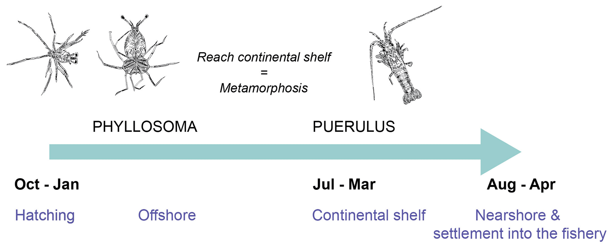
Figure 1 Early life cycle schematic of P. cygnus. Below the arrow indicates each stage's approximate timing (black) and location (blue). Above the arrow displays their growth, image credit Alice Ford.

Between November and February, berried western rock lobster females release their larvae (phyllosoma) throughout the study region (Figs. 1, 2a). They are then transported offshore by the prevailing currents into the open ocean, where they transform through a series of temperature-dependent moults (Fig. 1). They undergo their final metamorphosis into the actively swimming nektonic puerulus after approximately 8 months (Fig. 1). The onshore movement of puerulus across the continental shelf peaks between September and February (Phillips, 1981; de Lestang et al., 2018). Therefore, circulation patterns of the southeast Indian Ocean influence spatially varied cross-shelf transport of the puerulus (Caputi, 2008; Feng et al., 2011). After a maximum of approximately 30 d, they reach shallow areas of reef and seagrass habitats as early juveniles (Feng et al., 2011).

In the late 1960s, puerulus collectors resembling artificial seaweed were developed and deployed at several shallow-water sites within the fishery (Phillips, 1981). Puerulus are currently counted at eight sites spanning the latitude of the fishery, with the centrally located Dongara collectors (Fig. 2a) now providing over 50 years of in situ data (Kolbusz et al., 2021). The puerulus settlement index (puerulus index, PI) is derived from these data, with the majority of puerulus settlement occurring between August and January (de Lestang et al., 2012). Therefore the puerulus settlement season occurs between May and April.

Research on the interaction between the physical environment and PI began in the 1980s with a strong positive relationship found between the strength of the Leeuwin Current (LC), with Fremantle mean sea level (FMSL) as a proxy (Pearce and Phillips, 1988; Lenanton et al., 1991). Consequently, La Niña phases were also found to coincide with an above-average PI, thought to be due to a strengthened LC during these phases, with the Southern Oscillation Index (SOI) as an indicator of El Niño–Southern Oscillation phases (Clarke and Li, 2004; Caputi et al., 2001; Pearce and Phillips, 1988). These relationships were identified through long-term correlations between the PI, FMSL, and SOI (Fig. 3). Since 1988, studies have also demonstrated that the inter-annual variation in PI was influenced by the sea surface temperature (SST) and westerly (onshore) winds (Caputi and Brown, 1993; Caputi, 2008; Caputi et al., 2010). Caputi et al. (2001) defined a significant area overlapping with the spatial extent of the LC, where SST (27–34^∘ S, 105–117^∘ E) in February–April had a positive relationship with the PI of the subsequent season. The bottom temperature during the spawning season has also been identified as a cue for hatching and therefore has a possible influence on the puerulus settlement season to follow (Chittleborough, 1975; de Lestang et al., 2015).

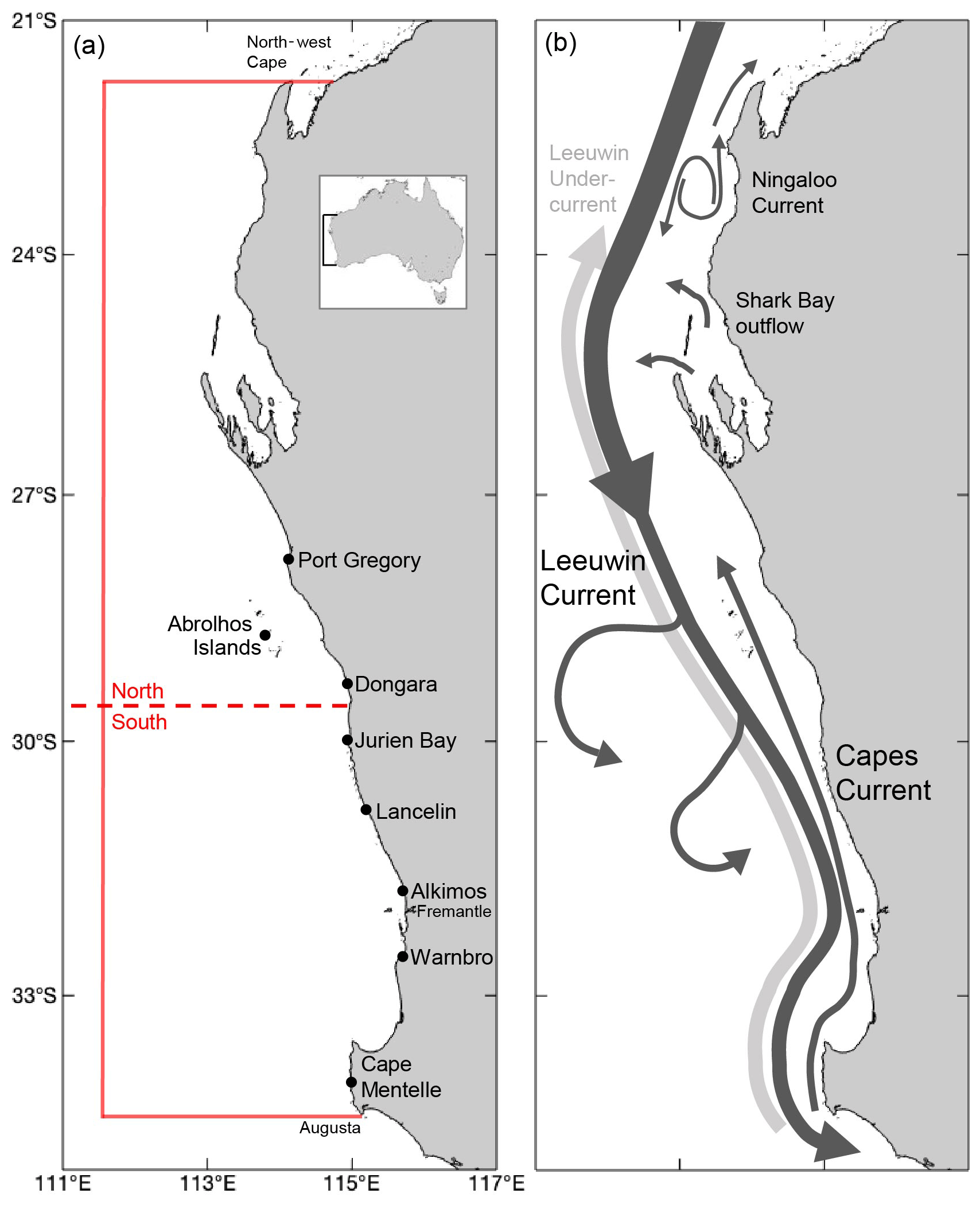
Figure 2 (a) Locations of puerulus survey sites included within this study and other locations of note. The north and south refer to the midpoint used in this analysis. The red boundary is the extent of environmental variables. The inset shows the location of the coastline in Australia. (b) Schematic of the major current systems thought to influence early-stage P. cygnus larvae movement. Relative arrow size and location show characteristic currents. Eddies generated by the LC flow down the continental shelf are also indicated.

Following the decline in the PI in 2008 and 2009 (Fig. 3), the aforementioned relationships between the PI and oceanographic factors broke down (de Lestang et al., 2015; Caputi et al., 2014; Feng et al., 2011). Through one of the strongest La Niña phases on record (2011), the PI still did not recover to the previously expected high values (Boening et al., 2012; Benthuysen et al., 2014). These changes have been generally attributed to increasing water temperatures during the spawning period, resulting in an earlier onset of spawning, and a decrease in the number of storms occurring near puerulus settlement (de Lestang et al., 2015). Since this decoupling between proxy parameters and PI, additional years of contrasting settlement have been recorded, thus providing a larger dataset to re-examine these relationships following the period of low settlement.

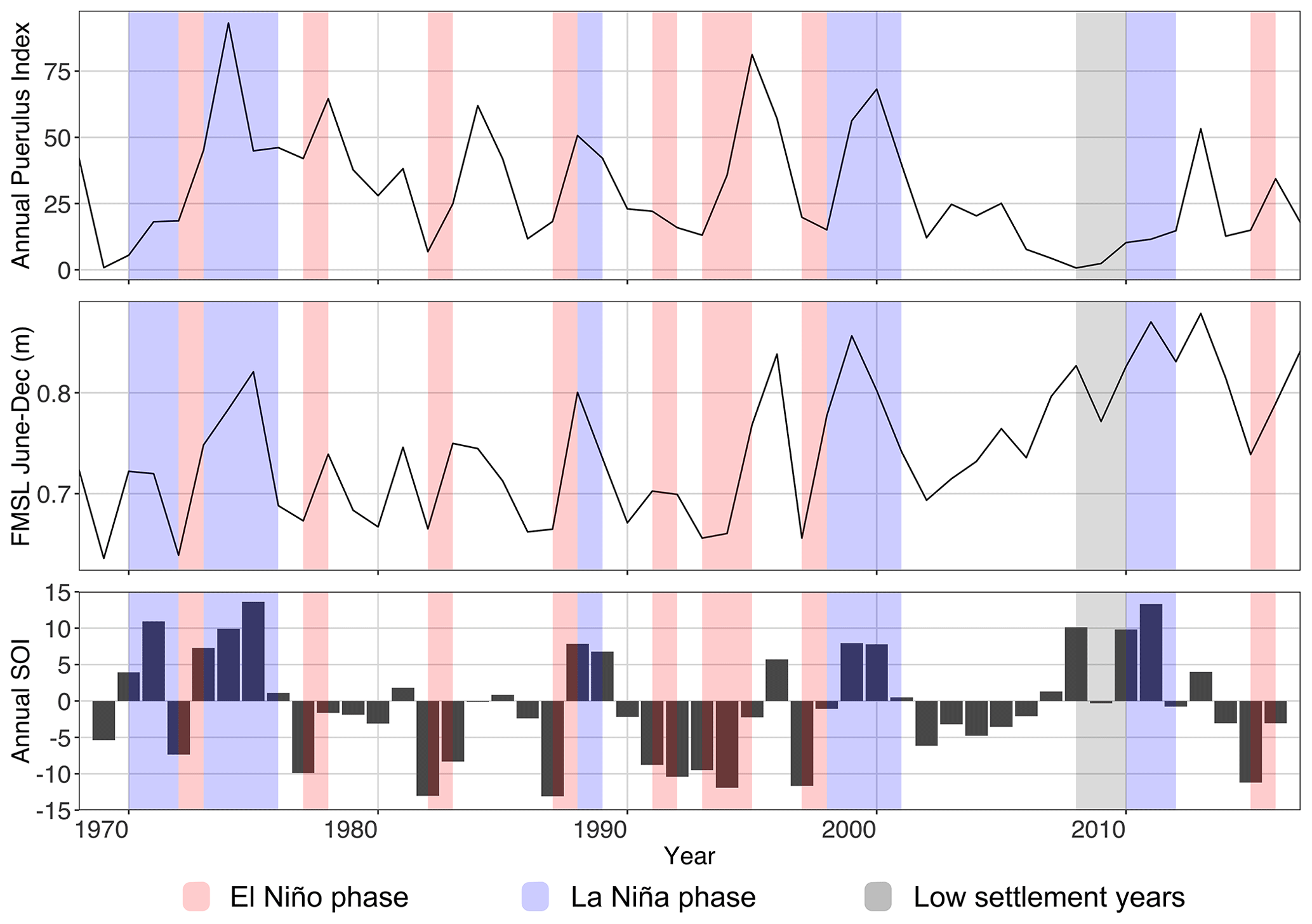
Figure 3 Time series of annual (a) fishery-wide PI (May–April), (b) Fremantle mean sea level (FMSL) over June to December (m), and (c) Southern Oscillation Index (SOI) (May–April). Grey shaded seasons indicate the less-than-expected PI based on a priori relationships (Caputi et al., 2001). Blue and red shading indicate a La Niña and El Niño periods, respectively. Updated to 2018 and modified from Fig. 5 in Caputi et al. (2001).

This study aims to understand the recruitment failure and subsequent shifts in settlement patterns, particularly regarding direct physical oceanographic parameters over the 9 to 11 months before settlement. Previous research had highlighted that the causal factor of the correlation between the LC strength and PI before 2009 was unclear. Several suggestions have been made as to whether it was due to the warmer waters the LC brings, high eddy retention of larvae close to the coast, or better nutritional development within eddies (Caputi et al., 2001; O'Rorke et al., 2015; Wang et al., 2015; Lenanton et al., 1991). Other parameters defining the oceanographic conditions in the region, including the northward-flowing Capes Current (CC) (Fig. 2b), cross-shelf flows, and kinetic and eddy kinetic energy, have been previously suggested as influencing the PI but not investigated (Hood et al., 2017; Koslow et al., 2008). The recent availability of high-resolution 3D numerical oceanographic model output over an extended period (Wijeratne et al., 2018) eliminates the need to use proxies to represent oceanographic processes. Therefore, we were able to calculate directly predicated oceanographic parameters at various locations throughout the fishery to investigate alongside puerulus settlement.

2 Study region

Water circulation off the west coast of Australia is driven by the Leeuwin Current (LC) system that incorporates the Leeuwin Current, the Leeuwin Undercurrent and summer wind-driven currents, and the Capes (CC) and Ningaloo (NC) currents, on the continental shelf (Fig. 2b) (Woo and Pattiaratchi, 2008; Pattiaratchi and Woo, 2009). The LC is generated through a meridional pressure gradient resulting from the difference between lower-density water off northwest Australia and the denser water of the Southern Ocean (Hamon, 1965; Pattiaratchi and Buchan, 1991; Pearce and Phillips, 1988). The mean southward volume transport of the LC peaks around 32.8^∘ S due to South Indian Counter Current input (Wijeratne et al., 2018). Near 28^∘ S statistical analysis has shown a break-point in the LC, suggesting responses from the current's forcing along the coastline may differ on either side of this latitude (Chittleborough, 1976; Berthot et al., 2007). The El Niño–Southern Oscillation (ENSO) cycle causes the pressure gradient to decrease (increase) during an El Niño (La Niña) episode, resulting in a weaker (stronger) LC and cooler (warmer) sea surface temperature SST (Pattiaratchi and Buchan, 1991; Feng et al., 2003; Wijeratne et al., 2018). This is supported by strong correlations between the Southern Oscillation Index (SOI as an indicator of ENSO phases) and LC transport at 34^∘ S with a 6-month lag (Schiller et al., 2008).

The LC is stronger during austral winter (May–July) and weaker during the austral summer (November–March) due to variations in the equatorial wind stress and the Australasian monsoon season (January–March) (Pattiaratchi and Siji, 2020; Pattiaratchi and Woo, 2009; Smith et al., 1991; Wijeratne et al., 2018). A weaker secondary peak in the LC also occurs over December–January (Wijeratne et al., 2018). During the summer months, southerly wind stresses overcome the alongshore pressure gradient, moving upper layers offshore and favouring upwelling onto the continental shelf (Pearce and Pattiaratchi, 1999). The CC can be identified through cooler waters initiated around 34^∘ S with the cooler water extending to 27^∘ S inshore of the LC (Fig. 2b) (Gersbach et al., 1999). The LC migrates offshore and is weaker over these sea-breeze-dominated summer months, whereas, during winter, it floods the shelf and dominates the distribution of water masses (Cresswell et al., 1989; Pattiaratchi et al., 1997; Woo and Pattiaratchi, 2008).

Mesoscale eddies have been identified in the LC system for more than 30 years (Andrews, 1977; Pearce and Griffiths, 1991; Cosoli et al., 2020). The LC, and its associated flows, becomes unstable with the significant variations in topography over the latitudinal extent of the current, generating eddies, meanders, and offshoots (Batteen et al., 2007). Therefore, as the LC strength increases, the system becomes more unstable, causing kinetic energy to increase (Feng et al., 2005; Pattiaratchi and Woo, 2009). The Abrolhos Islands at 28.8^∘ S and the narrowing of the continental shelf slope south of Dongara and the Perth Canyon are major topographic features for the preferential generation of these eddies (Fig. 2b) (Feng et al., 2005; Meuleners et al., 2008; Rennie et al., 2007; Huang and Feng, 2015; Cosoli et al., 2020). They have a mean radius of ∼ 100 km and generally keep their original formation shape, lasting approximately 8 months (Fang and Morrow, 2003; Cosoli et al., 2020).

3 Methods

3.1 Puerulus settlement data

Puerulus settlement is surveyed year-round, currently at eight sites across the fishery (between 34–27^∘ S) using artificial seagrass-like collectors (Fig. 2a). Sampling is conducted as close as possible to the full moon but may occur 5 d on either side of it. Therefore, puerulus are likely to have settled on the previous new moon period, giving approximately monthly data (de Lestang et al., 2012). The monthly puerulus settlement at each site is calculated as the average number of puerulus per collector. For this study, we used the puerulus settlement data from the 2001/02 season to 2016/17 at each of the eight sites (Fig. 2), aligned with high-resolution oceanographic data hereafter detailed and estimates of western rock lobster spawning biomass. Puerulus settlement data for each site were split into “early” (May–October) and “late” (November–April) portions, as described by Kolbusz et al. (2021).

3.2 Oceanographic data

To explore the variation in puerulus settlement, alongside the prevailing oceanographic conditions, a single value for the respective early or late portion of the season was determined. Where relevant, the oceanographic variable was the same for both portions.

3.2.1 Numerical model outputs

The Regional Ocean Modeling System (ROMS) has been used in hindcast mode (past-time) for the whole of Australia (ozROMS) to resolve subsurface and surface currents and the associated volume transports (Wijeratne et al., 2018). This is a fully three-dimensional circulation model, resolving processes along the continental shelf, including tides, setting it apart from other ocean models for the same region. The grid was set at a horizontal spacing of 3 km to allow for topographic detail, providing predicted water movement. At the time of writing, ozROMS model output was available for the period 2000–2017. Details and validation of the model are described by Wijeratne et al. (2018). Examination of this predicted dataset allows for the strength of the Leeuwin Current (LC), Capes Current (CC), and cross-shore transport to be determined, as well as estimates of kinetic energy (KE) and eddy kinetic energy (EKE) (Pattiaratchi and Siji, 2020). Their fluctuation is indicative of the conditions off the west coast of Australia.

Monthly surface KE and EKE were calculated from ozROMS to characterize the variability in the currents. A monthly time series was estimated following Eq. (1) for KE and Eq. (2) for EKE:

$$\begin{array}{}\text{(1)}& {\displaystyle }\text{KE}=\sqrt{{\displaystyle \frac{u^{\mathrm{2}}+v^{\mathrm{2}}}{\mathrm{2}}}},\text{(2)}& {\displaystyle }\text{EKE}=\sqrt{{\displaystyle \frac{{u^{\prime }}^{\mathrm{2}}+{v^{\prime }}^{\mathrm{2}}}{\mathrm{2}}}},\end{array}$$

where u and v are the monthly mean meridional and zonal velocities, respectively (Caballero et al., 2008), and u and v are the monthly averages with the climatological means subtracted to remove seasonality (Luo et al., 2011). The months that phyllosoma are offshore, depending on when they have hatched, can be between October (year − 1) and March (year + 1) (Fig. 2). Therefore, the calendar year from January to December was used to obtain an average for the offshore conditions spanning the possible time frame offshore. Due to different mean oceanographic conditions, we considered a north and south offshore box (Fig. 2a) that covered the approximate extent of where phyllosoma are transported (Feng et al., 2010, 2011; Berthot et al., 2007). For our analysis, we have not defined the directionality and size of eddies. Still, it is an important consideration pertinent to larvae energy stores that would require further modelling outside the scope of the current study (Cetina-Heredia et al., 2019b).

The monthly transport estimates of LC and CC (in sverdrups, Sv = 10⁶ m³ s⁻¹) were derived using the ozROMS hindcast dataset (Wijeratne et al., 2018). The transport for each current was defined as follows: (1) CC as northward volume transport of water across latitudes 27, 30, and 34^∘ S in water depths less than 100 m and (2) LC as southward volume transport of water across latitudes 27, 30, and 34^∘ S but in water depths greater than 100 m but limited to the upper 300 m of the water column (Table A1, Appendix A). For the LC austral winter strength, the transport over June, July, and August was averaged, and for summer December, January, and February were averaged. The LC summer period corresponds to recently hatched larvae (spawning season, s − 1), leaving the continental shelf and puerulus returning in the late portion of the season (settlement season, s) (Fig. 2). The LC winter period corresponds to when puerulus are returning to the shelf (settlement season, s). The CC strength was divided into early (September, October, and November) and late (December, January, February, and March) and corresponded to the time when recently hatched larvae were leaving the continental shelf (spawning season, s − 1) and puerulus were returning in the early and late portions of the settlement season respectively (Fig. 2).

Cross-shelf transport (in sverdrups) was calculated for each monthly time step between the depth contours (200–50 m) over 2^∘ latitudinal bins (26–28, 28–30, 30–32, and 32–34^∘ S) (Table A1, Appendix 1). These latitudinal bins were chosen closest to account for differences in topography and cross-shelf flow differences across the survey sites. Monthly averages for each latitudinal bin indicated that the variability in transport is highest over April to September. These months correspond to the eastward “on” movement of puerulus. Recently hatched larvae cross the shelf (westward, “off” in the spawning season) to the open ocean between September and March (Fig. 2). These two sets of months were averaged to get values of cross-shelf transport (as phyllosoma “off” and as larvae “on”) for each season (Fig. 2).

Temperatures in the model layer immediately above the seabed (“bottom temperature”) over the spawning depths (40–80 m) were retrieved from ozROMS due to the absence of in situ data (de Lestang et al., 2015). The predicted values were averaged over a northern and southern subset (Fig. 2a) of the whole spawning season (September–March). Due to the ozROMS hindcast starting in 2000, values were only available from the 2001 season since the spawning season is the calendar year prior to settlement. Despite de Lestang et al. (2015) using monthly values, we found only a small amount of variation between the months and therefore used a single bottom temperature value to represent a season. The temperature in the top 100 m of the water column, east of 108^∘ E, as a mean annual value from ozROMS was also included. This accounts for temperature variation over the migrating depths phyllosoma occupy over their early pelagic life cycle (Griffin et al. 2001; Feng et al. 2011).

3.2.2 Satellite-derived sea surface temperature (SST)

Satellite-derived SST data for the study region were obtained from the Integrated Marine Observing System (IMOS) Australian Ocean Data Network (AODN) portal (https://portal.aodn.org.au/, last access: 1 March 2021). The climatology data, centred on the base period 1993–2020, SST Atlas of Australian Regional Seas (SSTAARS) (Wijffels et al., 2018), were used to derive monthly SST anomalies for the region extending offshore to 108^∘ E (extent in Fig. 2; see also Pattiaratchi and Hetzel, 2020). This was to reflect the extensive duration (∼ 9 months) of the pelagic larval and pre-settlement stage of P. cygnus (Phillips, 1981). All monthly SST anomalies were initially included in the analysis due to the likely importance of temperature on all stages of the pelagic larval stage (Caputi et al., 2001; de Lestang et al., 2015).

3.3 Independent breeding stock survey (IBSS)

Independent breeding stock surveys (IBSSs) have been conducted annually since 1992 over the last new moon (∼ 15 November) before the start of the fishing season (de Lestang et al., 2018). The catch rates of spawning females from this survey (adjusted for fecundity) provide a standardized egg production index. It is conducted at up to six sites spanning the fishery and close to the peak in egg production (November) (Caputi et al., 1995; Chubb, 1991; de Lestang et al., 2016). Therefore, IBSS was included in our analysis, accounting for variability in the number of hatching larvae.

3.4 Generalized additive modelling

The oceanographic variables likely to influence water movement and the distribution and survivorship of P. cygnus, detailed above, were considered predictors of the puerulus settlement within a generalized additive model (GAM). In addition, the IBSS was included as a predictor to include variability in the number of hatching larvae. Due to the extensive latitudinal range of the settlement data, some environmental variables were dividing into northern, central, or southern areas depending on the data type and availability. A value was obtained for each possible predictor variable to align with each half of the puerulus season (Appendix A, Table A1). Firstly, linear regression analysis was performed to assess whether strong (> 0.70) correlations existed between variables. Where valid, a case-by-case approach was taken to determine whether both, an average, or one of the two variables was included in the overall model before the time series modelling – this eliminated potential problems with collinearity and overfitting (Graham, 2009). Bottom temperatures were all highly correlated (> 0.89) and therefore averaged to give a single variable. Co-correlation between the SST of adjacent months led to a winter and summer average being used.

GAMs with full subset model selection (FSSgam) were used to investigate the influence of the final 16 (8, early and late settlement periods) different response variables (Fisher et al., 2018). Predictors were initially limited to a maximum of three knots per spline. However, due to the relatively small sample size and heterogeneous distribution of the predictors, cross-shelf transport remained, but other predictors were treated as linear relationships. Model sizes were limited to three predictors to prevent overfitting. Model selection was based on Akaike's information criterion (AIC; Akaike, 1973) optimized for small sample sizes (AICc; Hurvich and Tsai, 1989). The best models selected were the most parsimonious within two AICc units of the model with the lowest AICc (Burnham and Anderson, 2002). Importance scores for each variable were obtained by summing the AICc weights of each model that each variable occurred within (Fisher et al., 2018).

Table 1 shows each predictor variable and the associated hypotheses for each annual value. The LC consistently flows southwards and is strongest over the winter months, possibly flooding the shelf. Therefore, over the winter months, this would likely positively affect late-stage phyllosoma successfully reaching the nearshore. Over the summer months, the LC strength, if stronger, would likely impede the survival of early-stage phyllosoma (Feng et al., 2011). Given the stronger opposing LC, the northward-flowing CC on the shelf would likely positively impact puerulus settlement (Muhling et al., 2008). Kinetic energy will likely positively impact the transportation of phyllosoma throughout their early pelagic life cycle (Cetina-Heredia et al., 2019a; Hood et al., 2017). Similarly, cross-shelf transport offshore would likely increase the survival of phyllosoma, and cross-shelf transport onshore after the pelagic phase would assist puerulus transportation onshore. P. cygnus spawning likely occurs sooner with an increased bottom water temperature, causing possible timing mismatches over the next 9 to 11 months (de Lestang et al., 2015). Conversely, warmer water temperatures increase the rate of phyllosoma development, therefore likely increasing their survival (Phillips et al., 1978; de Lestang et al., 2015). If the IBSSs were higher, there would be more spawning stock and therefore likely an increase in phyllosoma and eventual puerulus (de Lestang et al., 2012). These variables resulted in a total of 39 possible predictors of the late puerulus settlement (eight sites) and 33 possible predictors of the early puerulus settlement at sites (eight) (Appendix A, Table A1). LC strength in summer and the late CC strength predictors for early settlement were omitted since they occur after early settlement each season. Given the predicted data availability and the spawning season being in the calendar year prior, the relationship between all predictors and puerulus settlement was limited to the 2001 to 2017 seasons.

The R language for statistical computing (R Core Team 2018) was used for all data manipulation (dplyr; Wickham et al. 2018) and analysis (Wood, 2017) (mgcv; Wood, 2011). In addition, MATLAB and the M_map toolbox were used for any spatial plotting (MATLAB, 2019b; M_Map: A mapping package for MATLAB, Version 1.4 m).

3.5 Exploration of variation in oceanographic conditions

Seasonal and inter-annual variability, not captured within the GAM, was explored graphically with the inclusion of moving means. An extended period of low activity was experienced in the southeast Indian Ocean between 2001 and 2007 (Pattiaratchi and Siji, 2020). Given that processes in the ocean do not respond instantaneously, these “hiatus” conditions were explored as a whole. ENSO information (SOI) and the Fremantle mean sea level (FMSL) were obtained from the Bureau of Meteorology (2022a, b). Altimeter data were accessed from the IMOS AODN to investigate the relationship between the PI and the energy system, in particular, the long-term KE and EKE over the southeast Indian Ocean (Pattiaratchi and Siji, 2020)

During the summer, the interactions between the Capes Current and Leeuwin Current were also addressed (Pattiaratchi and Woo, 2009). First, the LC and CC summer period strengths were standardized for each season, and then the difference between the two was plotted alongside the early and late puerulus settlement levels.

Table 1 Predictor variables and metrics used in the GAM analysis to investigate variability in puerulus settlement and associated hypothesis. The subscript s identifies the relativity of a month to the puerulus settlement season (May–April) in question. s − 1 is within the season prior and s + 1 is after. − denotes a negative relationship, and + denotes a positive relationship.

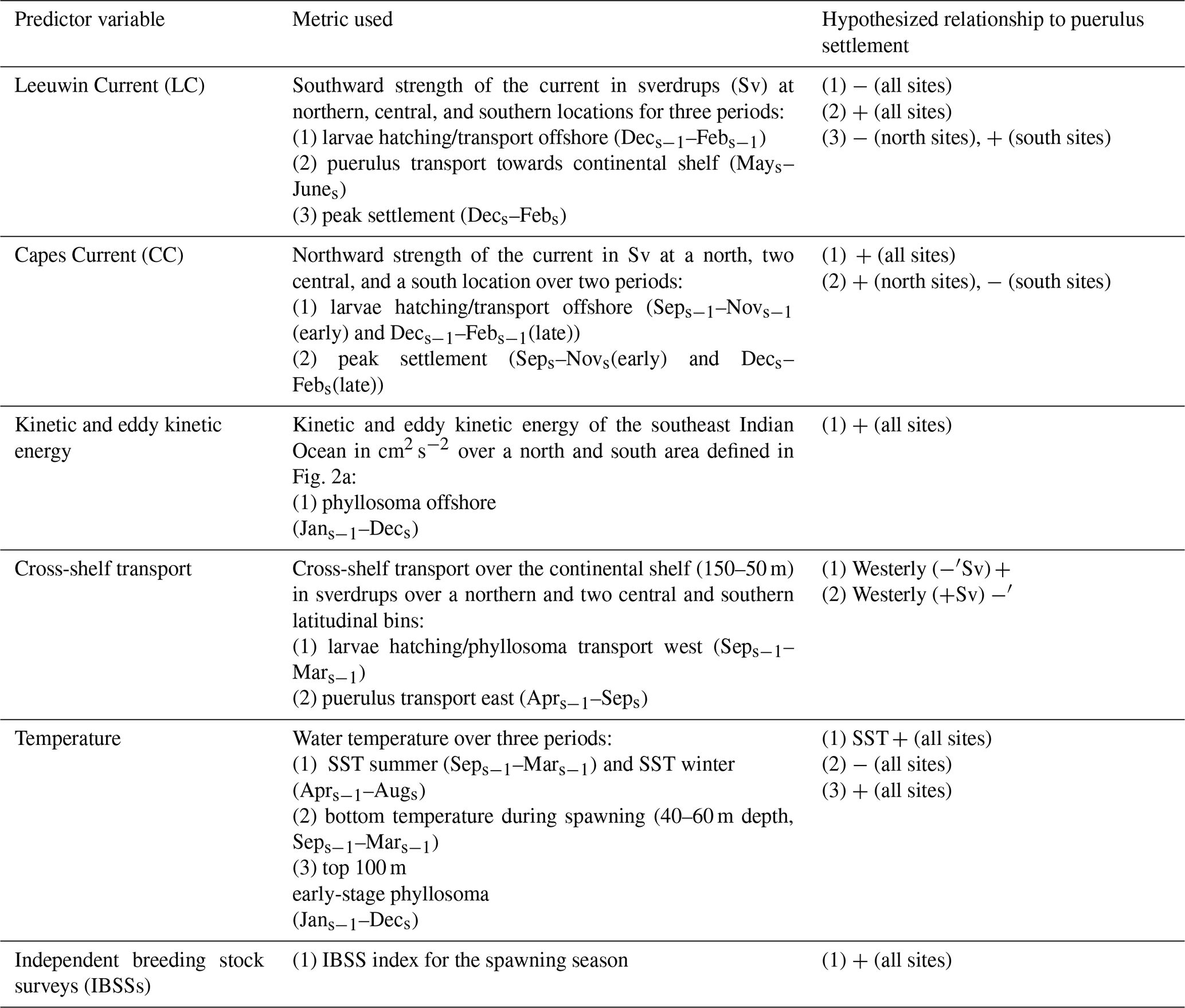
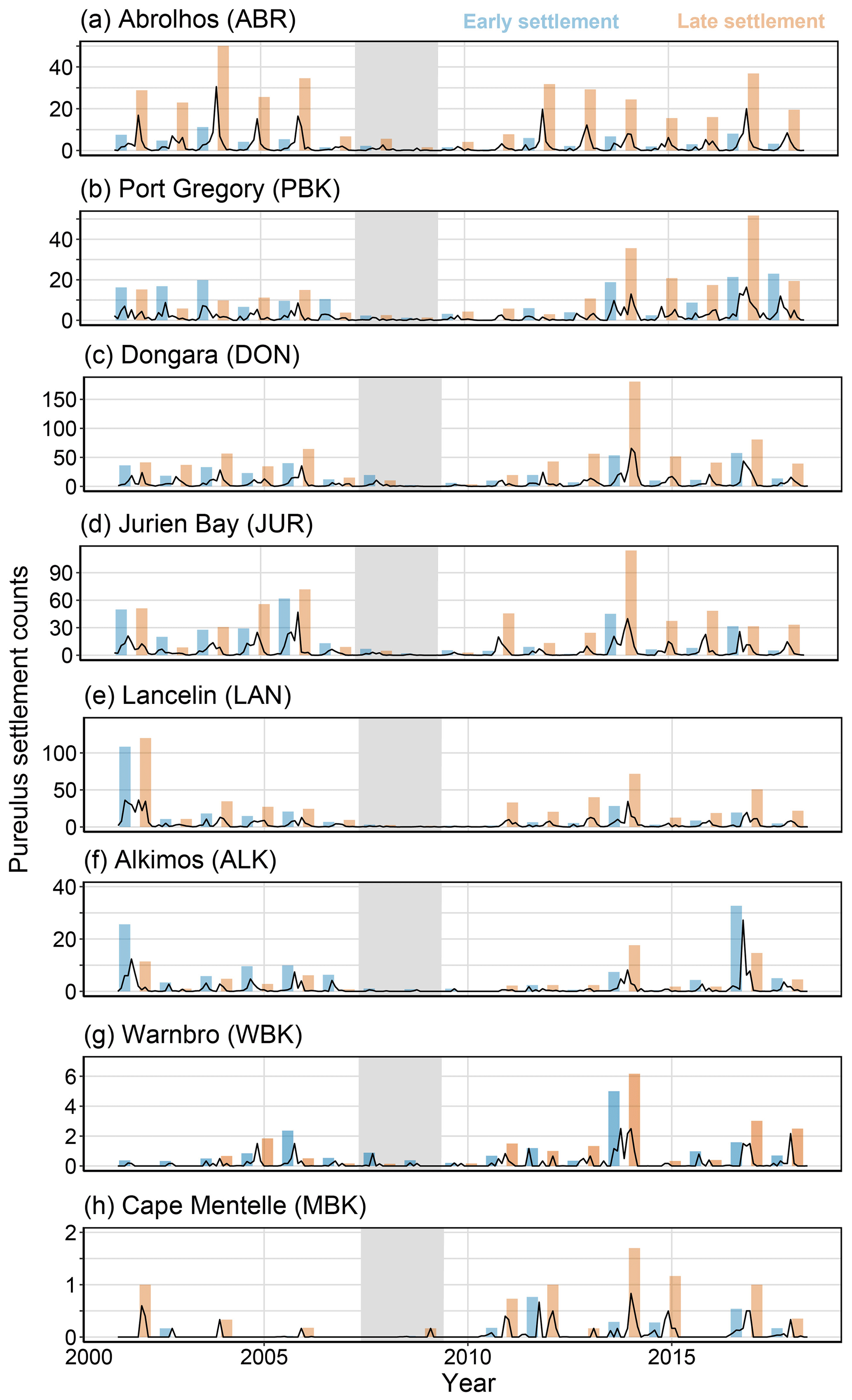
Figure 4 Monthly average puerulus counts for each monitoring site (black line) with the early (May–October, blue) and late (November–April, red) puerulus settlement for the season. The index is a sum of the included monthly average puerulus counts. Grey shaded seasons (2008 and 2009) indicate the less-than-expected PI based on a priori relationships (Caputi et al., 2001).

4 Results and discussion

Our findings demonstrate that similar oceanographic conditions influence adjacent puerulus monitoring sites. The Leeuwin Current strength over the summer months has increased since the low puerulus settlement season, alongside a decrease in the Capes Current, suggesting a mismatch in the puerulus transport processes. In addition, this period occurred alongside neutral ENSO conditions and cooler water over the likely P. cygnus pelagic distribution. These results and their discussion are in the following three sections: (1) time series exploration of P. cygnus settlement between 2001 and 2017 and associated oceanographic conditions experienced by the larvae to represent each puerulus settlement season (May to April), (2) exploring the correlation of oceanographic conditions with settlement data through a general additive model analysis, and (3) inter-annual and seasonal oceanographic variability.

4.1 Time series patterns

Puerulus settlement differs dramatically over the latitudes of the fishery, with central latitudes experiencing the highest numbers (Fig. 4). At the Abrolhos (Fig. 4a), the late settlement is consistently higher and remained consistent after the recruitment failure, which is expected (Kolbusz et al., 2021). Other sites display similar early and late puerulus settlements before 2008. However, after 2009, recovery occurs predominately in the latter half (Fig. 4a, c, d, and e).

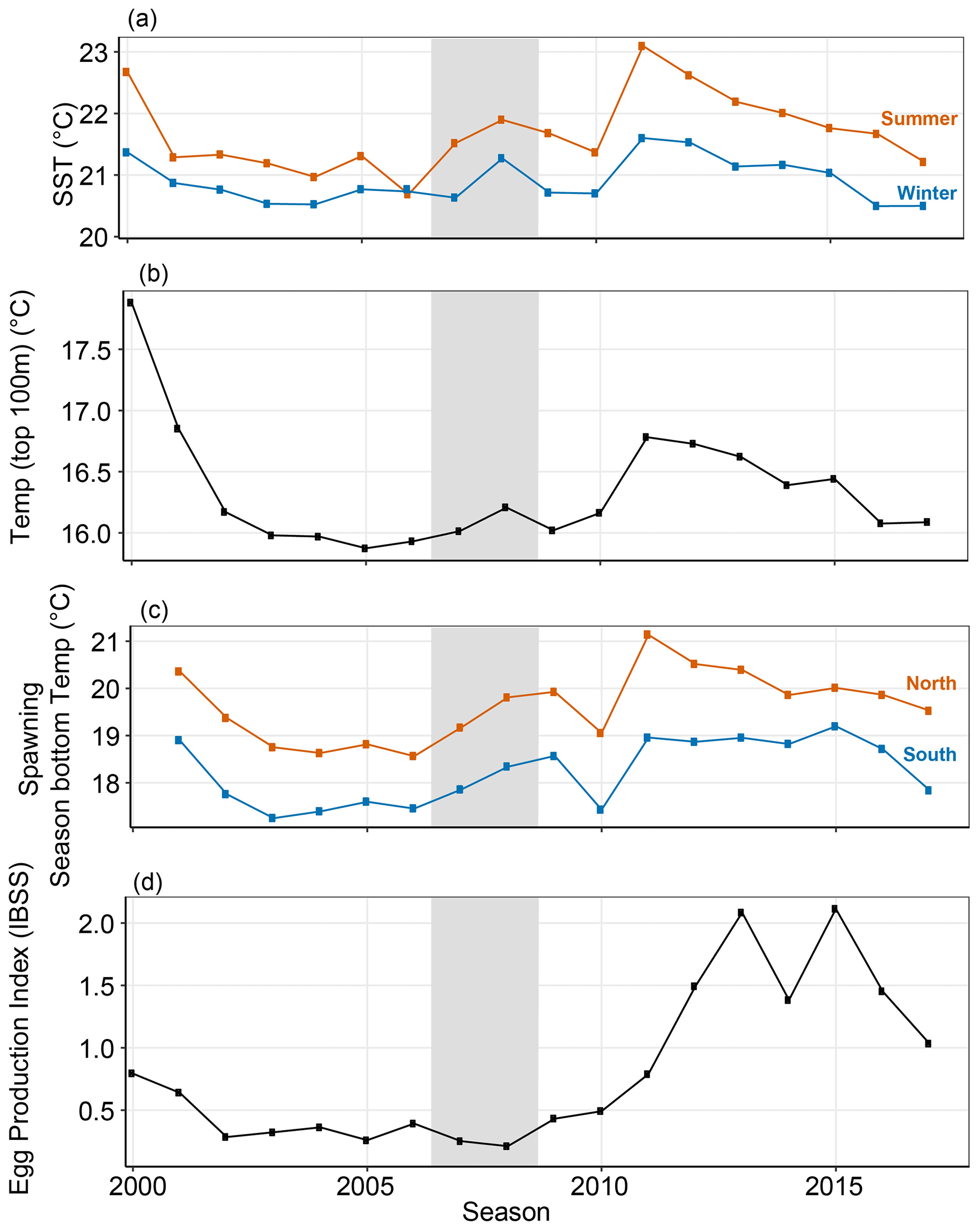
Figure 5 Parameters calculated for seasonal analysis of PI. (a) Sea surface temperature (^∘C) from 24–34^∘ S and out to 108^∘ E obtained from the SSTAARS daily dataset on the IMOS AODN portal from 1996 to 2016. (b) Temperature in the top 100 m of the offshore area from 24–34^∘ S and east of 108^∘ E over January–December, the average time phyllosoma are offshore. (c) Average bottom temperature (40–80 m depths) (^∘C) of the spawning season for associated PI season for October to March in the northern (blue line, shown in Fig. 2a) and southern latitudes (red line, shown in Fig. 2a) of the fishery. (d) The independent breeding stock survey index (IBSS) lagged 1 year to give a spawning stock index for the year prior (de Lestang et al., 2016). Grey shaded seasons (2008 and 2009) indicate the less-than-expected PI based on a priori relationships (Caputi et al., 2001).

The three temperature variables (SST, top 100 m temperature and bottom temperature) all followed a similar pattern to one another (Fig. 5a–c). They gradually decreased from highs in 2000 to a low in 2005 before slightly increasing from 2008, all reaching maxima in 2011 when a marine heatwave occurred in February (Wernberg et al., 2012). A decrease of approximately 1–2 ^∘C in bottom temperature during the spawning season was evident over the early 2000s, which shifted over the low-PI seasons (grey seasons, Fig. 5a–c). It then increased again by 2012 (Fig. 5). Until the heatwave, the variation in PI at some sites (Lancelin and Port Gregory) additionally aligned with the SST fluctuations. This is likely the bottom temperature variation captured by de Lestang et al. (2015). The winter months (June to August) had less than 1^∘ of between-year annual variability over the entire temporal scale.

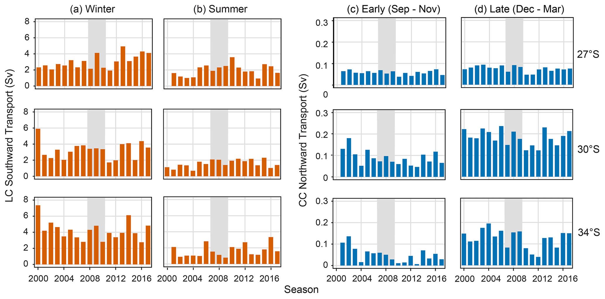
Figure 6 Leeuwin (LC) and Capes (CC) current strengths at 27, 30, and 34^∘ S. (a) LC (southward transport, Sv) over winter (May–July) and (b) summer (December–February). (c) CC (northward transport, Sv) (c) over the early portion of the summer (September–October) and (b) late portion of the summer (December–March). Grey shaded seasons (2008 and 2009) indicate the less-than-expected PI based on a priori relationships (Caputi et al., 2001).

The IBSS was consistently under 0.5 from 2002 until the 2011 season before increasing 3-fold by 2013 to record highs (Fig. 5) (de Lestang et al., 2016). Previous studies have not found the IBSS to be implicated in the recruitment failure (de Lestang et al., 2015). However, it was included in the current analysis for completeness and because studies of recruitment failures in other fisheries have frequently suggested spawning biomass to be a factor (Guan et al., 2019; Ehrhardt and Fitchett, 2010). In addition, the IBSS increased from 2011; this is likely due to the restrictive fishery management. After the lower-than-expected puerulus settlement in 2008 and 2009, restrictions to fishing were designed to preserve spawning biomass. Therefore the IBSS was expected to increase.

The LC was the strongest over the winter months, reaching 7 Sv in the 2000 season at 34^∘ S (Fig. 6a). However, the summer LC was strongest in 2010, at 27^∘ S. Both values align with strong La Niña conditions (Boening et al., 2012). This maximum, however, did not correspond to a maximum in winter LC strength (Fig. 6b) (Wijeratne et al., 2018). Over the initial months of the CC forming (Fig. 6c), it is, on average, strongest at 30^∘ S. The CC displayed a roughly similar pattern across all latitudes with less variability in current at 27^∘ S where it is weakest (Fig. 6c and d). CC minima occur over the 2010 to 2012 seasons in the early and late strength signals (Fig. 6c and d). Spatial variations in the LC and CC were distinguishable with increased LC at the southern latitude (Fig. 6a and b) and the strongest CC signature at 30^∘ S (Fig. 6d) as reported previously by Wijeratne et al. (2018).

Water circulation at all latitudes of the fishery was predominantly driven by the LC, with the changing topography down the coast causing less onshore flow on average within the centre of the fishery (29^∘ S) (Rennie et al., 2007; Feng et al., 2010; Wijeratne et al., 2018). Regions with a wider continental shelf generally have higher retention of waters, therefore causing less cross-shelf transport of water. Depth-averaged cross-shelf transport of water was predominantly onshore at both 33 and 29^∘ S (Fig. 7). This was not unexpected given the steep topography of the continental shelf and LC interactions. Average monthly variations in cross-shelf transport indicated that between April and September onshore transport increased at 33 and 29^∘ S; however, it decreased at 31 and 27^∘ S (Fig. 7). Coastal geographic features increase the spatial heterogeneity over the latitudes and how the LC interacts with the nearshore (Feng et al., 2010). At 27^∘ S, on average offshore transport was possibly due to more mixing and a wider continental shelf. This is due to the topography of Shark Bay and the contribution of the Ningaloo Current (Fig. 2b), likely playing a role (Woo and Pattiaratchi, 2008).

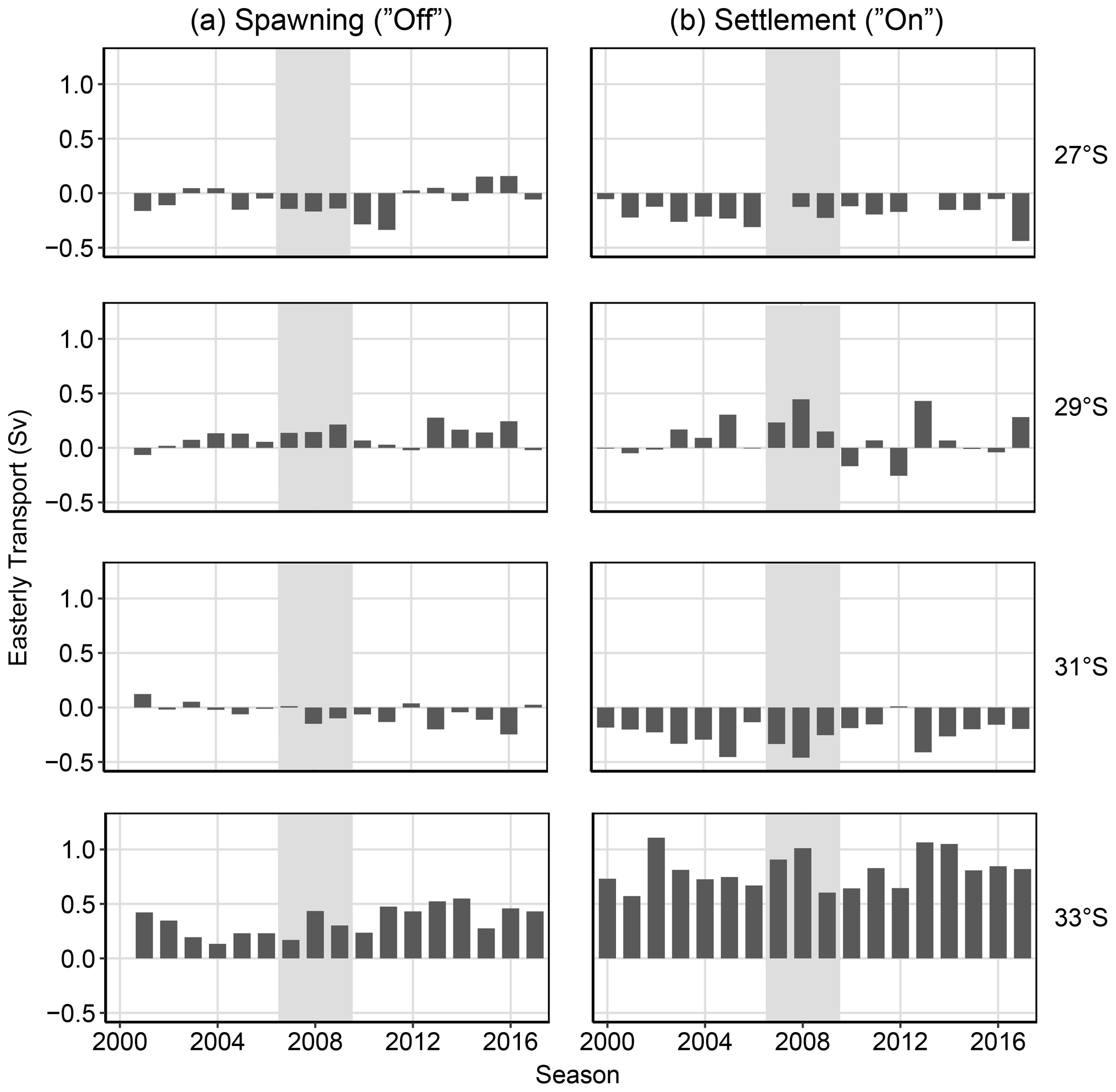
Figure 7 Cross-shelf transport (easterly) between 200–50 m over 2^∘ latitudinal bins (26–28, 28–30, 30–32, and 32–34^∘ S). Averaged for the (a) spawning “off” transport season (September–February, season −1) and (b) settlement “on” transport season when variation in cross-shelf transport is the highest (April–September). Grey shaded seasons (2008 and 2009) indicate the less-than-expected PI based on a priori relationships (Caputi et al., 2001).

Variations in EKE and KE over the time series show approximately 5-yearly patterns (Fig. 8) in fluctuation with maxima in 2000, 2005, and 2011 aligning with ENSO events (Pattiaratchi and Sijim 2020). From 2002 to 2008, the KE and EKE were relatively low, indicating a weaker LC over those seasons. Particularly over the southern box, the decrease in KE and EKE and recovery by 2012 show similar patterns to the puerulus settlement (grey years, Fig. 8c and d). Additionally, the southern box shows increased variability, suggesting greater variability in the LC at southern latitudes (Fig. 8c and d). Conversely, the northern values, particularly for KE, increased over the same time frame, with less variability (EKE), indicating that different forcing mechanisms, such as the South Indian Countercurrent, may play a role (Fig. 8c and d).

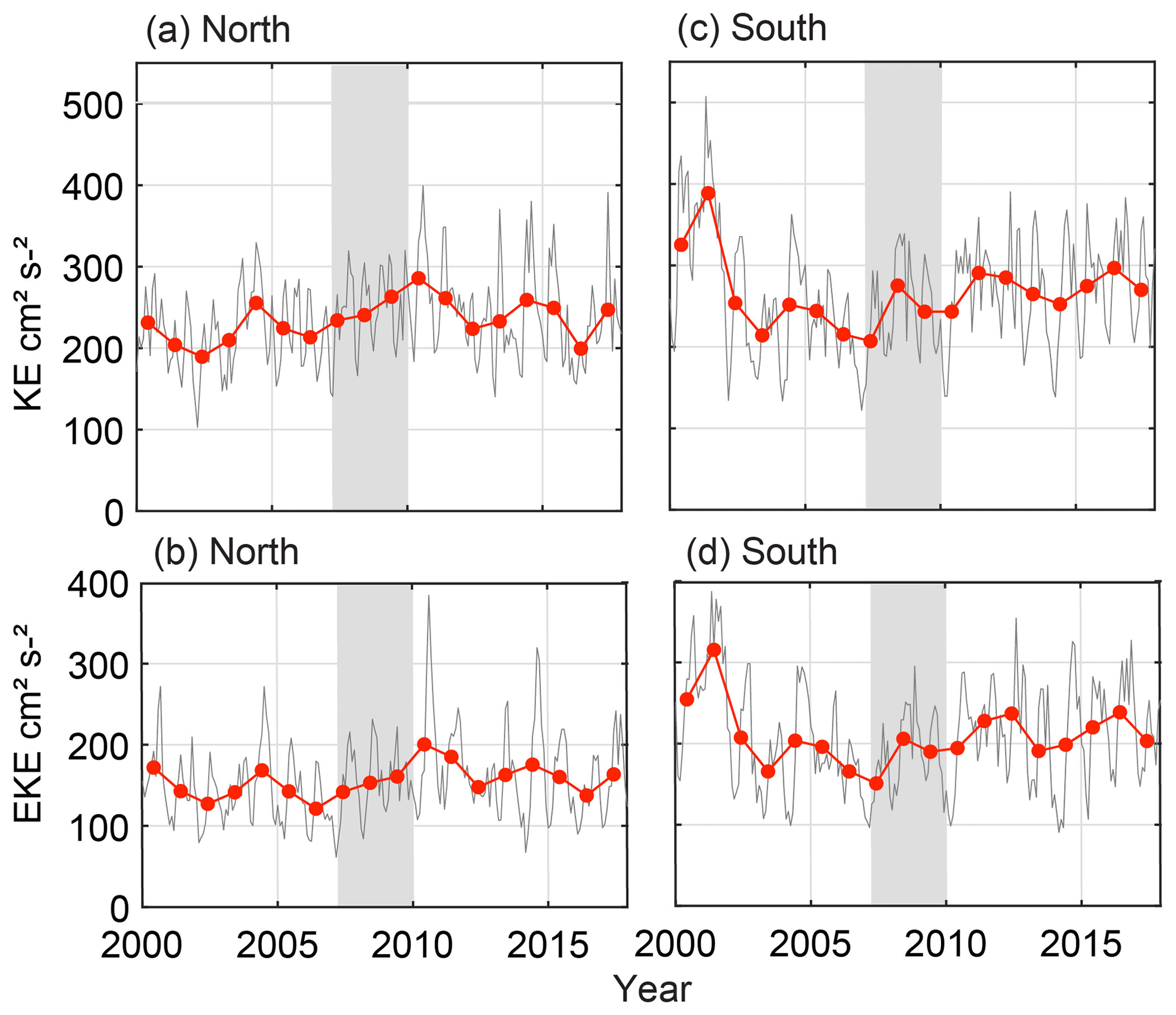
Figure 8 Monthly kinetic energy and eddy kinetic energy (grey) with yearly averages (January–December) (red). North and south divides are shown in Fig. 2a. (a) KE (cm² s⁻²) in the north. (b) EKE (cm² s⁻²) in the north. (c) KE (cm² s⁻²) in the south. (d) EKE (cm² s²) in the south. Grey shaded years (2008 and 2009) indicate the less-than-expected PI based on a priori relationships (Caputi et al., 2001).

4.2 Generalized additive model

The generalized additive model (GAM) analysis shows that puerulus settlements at adjacent sites tend to be influenced by similar oceanographic variables. However, the Abrolhos (northernmost and offshore) and Cape Mentelle (southernmost) sites are unique (Fig. 9, Appendix B). The most significant relationships did vary between the early and late portions of the seasons and between sites, as expected (Table 1). Those of note are discussed hereafter.

In contrast to our predictions (Table 1), sites were correlated by a negative relationship to KE in the north for early settlement (Fig. 9a). This correlation was more robust for the northern sites. A strong KE implies a strong LC signature over the defined spatial area (Fig. 2a). Comparatively, EKE and KE in the south had positive relationships to sites in the centre of the fishery for early and late settlement, suggesting a different forcing could be at play (Fig. 9). This was alluded to within the time series analysis (Fig. 8). The possibility that two adjacent parts of the southeast Indian Ocean would have opposing effects on the settlement at only two locations appears spurious. However, the southern and central flows of the South Indian Countercurrent (sSICC, cSICC) flow eastward within the southern and northern KE “boxes” respectively (Menezes et al., 2014). These current jets connect with the LC and may cause the temporal and spatial difference in KE and subsequent influences on puerulus settlement. In particular, for the Abrolhos, KE in the north is within the most parsimonious model for early and late settlement. Due to the sites' location offshore, increased water movement may prevent puerulus from successfully settling on the islands within the defined area of KE. Instead, they could swim elsewhere with less resistance. This difference in KE relationships suggests different driving mechanisms over the fishery on both the temporal (early and late) and spatial (north and south) scales.

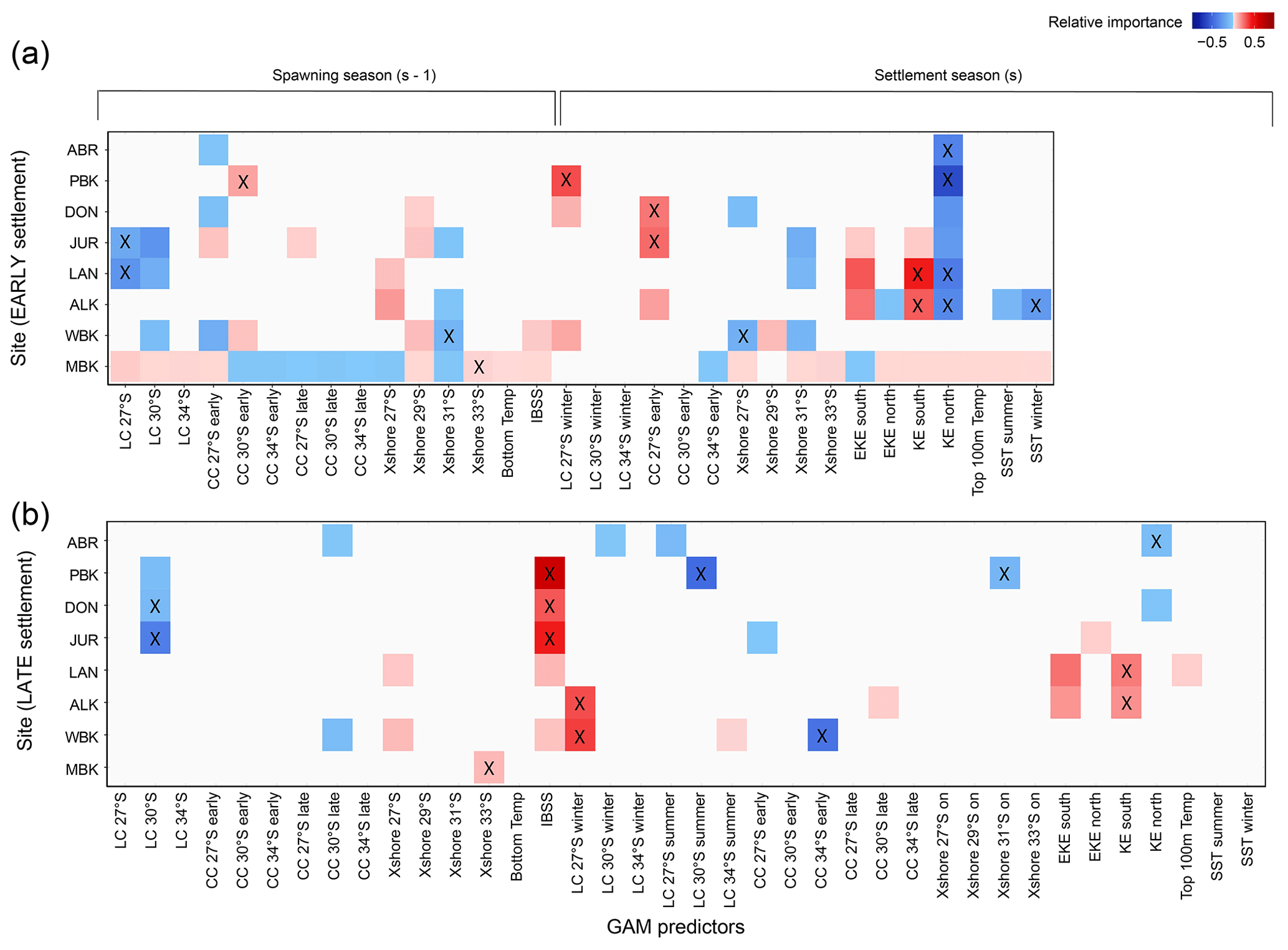
Figure 9 Variable importance scores within 2 AIC of the top model from the multiple linear regression analysis (GAM) to predict the (a) early and (b) late settlement at sites. Full results are in Appendix Tables B1 (early) and B2 (late). The timeline (above) indicates the timing of the variables from either the spawning season (s − 1) where larvae are moving offshore (westward) or the settlement season (s) where larvae are moving eastward. Positive (red), zero (white), and negative (blue) relationships with variables are shown, and variables within the most parsimonious model for each site are indicated (X).

The model results provide clues regarding the influence of the LC and CC (LC winter, LC summer, CC early and late) on phyllosoma when they are in later life stages. Interestingly, the LC during the spawning season at 27^∘ S was within the most parsimonious model for Lancelin early settlement as a negative relationship (Fig. 9a). Thus, for Lancelin, the LC may have been too strong for some early-stage phyllosoma to cross the shelf, to get westward, without being swept too far south for survival. Especially given the steep continental shelf at this latitude. In winter, a stronger LC (puerulus reaching the continental shelf) and a stronger CC (puerulus settling on reefs) were suitable for early settlement at Dongara. This was a hypothesized result (Table 1) and was also consistent at adjoining sites (Port Gregory for LC and Jurien Bay for CC, Fig. 9a) (Pearce and Pattiaratchi, 1999). For later settlement, the opposite relationships occur. The LC in summer has a negative relationship to Port Gregory (and Abrolhos), and the CC has a negative relationship with Warnbro (Fig. 9b). This was expected for Port Gregory, a northern site, to be negatively influenced by the southward-flowing current (LC), transporting puerulus further southward. Similarly, southern sites are negatively influenced by the northward-flowing current (CC), transporting puerulus northward. However, these trends become vague over the central latitudes of the fishery where little to no relationship is found, especially during the summer of hatching (Fig. 9a, CC 27^∘ S early). This draws attention to the spatial and oceanographic heterogeneity of the study sites. Given the mix of expected and unexpected and strong and weak results from the multiple regression analysis, particularly for the early settlement, it is clear complex forcing's are at play in the system, with both currents flowing in opposing directions perpendicular to the direction puerulus are swimming. The influence of factors found to have the strongest correlation on puerulus settlement is presented in the following Sect. 4.3.

The IBSS shows a strong positive relationship with Port Gregory, Dongara, Jurien Bay, Lancelin, and Warnbro over the late settlement. However, it has little relationship with the early settlement (Fig. 9a and b). Nevertheless, these positive relationships corroborate that the egg production influences the number of larvae returning to the coast as puerulus and may more accurately represent the spawning stock of puerulus reaching the coast over the latter half of the settlement season. Given the longer time series available for the IBSS and Dongara settlement, we reanalysed the relationship for a more extended period. We found that pre-2000 IBSS is a reasonable predictor with an R² of 0.434 and explaining 30.3 % of the deviance in the Dongara settlement (Fig. 10). In an ideal scenario, one would expect all sites, both early and late, to have a relationship with the spawning stock. For locations where increased IBSS did not positively correlate with PI, it may be solely that the influence of oceanographic factors on the puerulus settlement was more substantial.

Cross-shelf transport shows irregular patterns between the sites. Cross-shelf transport for the spawning season (27, 29, and 33^∘ S, Fig. 9a) has some positive links to increased settlement in the early half of the season for sites south of Dongara. However, this is the opposite for 31^∘ S (Fig. 9a), but these relationships are less pronounced over settlement later in the year (Fig. 9b). Various transportation pathways are likely working in opposing directions to influence settlement at different locations. Average cross-shelf transport has previously indicated a break over the mid-latitudes of WA (Wijeratne et al., 2018, Fig. 9).

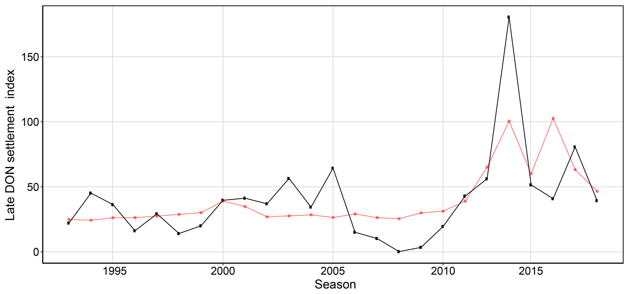
Figure 10 Observed (black) and modelled (red) late Dongara (DON) settlement index from 1993 to 2018. The red line is the most parsimonious model extended to 1993.

On an annual timescale, increased strength in KE in the northern offshore areas of the fishery (Fig. 1) was associated with a decrease in puerulus settlement in the early portion of the season. It is not uncommon for the advective behaviour of large-scale eddies to negatively affect crustacean species (Medel et al., 2018; Nieto et al., 2014). Retention and dispersal of larvae can also differ in persistent eddy scenarios where a more uniform shape likely leads to retention. However, a more eccentric shape leads to dispersal (Cetina-Heredia et al., 2019b). Earlier studies suggest an increase in the number of eddies positively influences the retention of larvae and, therefore, transport across the shelf and to the nearshore (Griffin et al., 2001; Yeung et al., 2001; Cetina-Heredia et al., 2019a, 2015). This is contradictory to our results. Our study used the mean annual KE over a large spatial area, and the site in question is north of the highest density of puerulus settlement. Using a large spatial area, we have omitted the influence of sub-mesoscale features within the region, which could impact a puerulus' ability to cross the shelf and reach coastal habitats (Cosoli et al., 2020).

The GAM analyses suggest that different environmental drivers influence PI at each site, but this varies depending on when puerulus return to shore (early or late, Fig. 9a, b). However, we can establish discernible patterns with some certainty and physical relevance. Sites closer in latitude have similar results, Abrolhos and Cape Mentelle being the exceptions. Abrolhos is located off the shelf and has historically had different trends in PI compared to other locations and even on the adjacent coast. The Abrolhos PI has also recovered to pre-failure levels, whereas coastal locations have not, particularly at Lancelin and locations further south (Kolbusz et al., 2021). Cape Mentelle has historically had a low settlement and also has a unique location being the farthest south. Early settlement at Cape Mentelle also showed little difference between all top models within 2 AIC of the most parsimonious model (cross-shelf transport at 33^∘ S during spawning season). Despite one variable having the highest importance and being in the top model, there was little difference between all models within 2 AICc units.

Given the several months over which lobster larvae hatch, followed by their prolonged pelagic life cycle and settlement estimated to occur some 9–11 months later (Phillips, 1981), the large amount of variation and lack of solid relationships between environmental or biological predictors and PI was not unexpected (Fig. 2). However, we have revealed patterns up and down the coast, suggesting that both biological and environmental predictors can have a strong and sometimes consistent influence on puerulus settlement for adjacent sites.

4.3 Variation in oceanographic conditions

All the oceanographic factors examined here have been suggested to directly influence P. cygnus larvae at some point in their first year of life. Over time, the forcing and interactions between these environmental variables were too complex to examine in the multiple regression analysis. However, they may have as much influence on successful puerulus settlement as instantaneous values used. Furthermore, the various oceanographic mechanisms act differently, sometimes in competition (Fig. 9a, b), to provide contrasting results for the different sites. Using the above multiple regression analysis results as an exploratory tool, we have additionally drawn upon patterns in the southeast Indian Ocean and WA coastal zone over the last 2 decades. This includes lagging conditions, alongside the fishery changes, that may have contributed to the “worst-case scenario” and resulted in the recruitment failure in 2008–2009.

4.3.1 Inter-annual: hiatus period and cross-shelf transport

Over the past 30 years, links between ENSO events and the PI have been well documented using the SOI (Fig. 3) (Caputi et al., 2001; Pearce and Phillips, 1988). Warmer temperatures are experienced during stronger LC conditions evident during the La Niña phase (positive SOI), providing better conditions for larval development. The SOI record since these relationships began highlights the possibility of sustained neutral ENSO conditions being a reason for this breakdown (Pattiaratchi and Hetzel, 2020; Pattiaratchi and Siji, 2020). From 2000 until 2009, neither a moderate La Niña phase nor a moderate El Niño phase occurred, and consequently, the energy in the system also decreased (Fig. 3). After 2009, an unusually strong LC (La Niña, 2011) was preceded by an unusually weak year (El Niño, 2010) (Huang and Feng, 2015). Before 2008 there were fluctuations in LC strength, or phases of moderate strength, over several seasons whilst the puerulus settlement also fluctuated similarly (Fig. 3, Caputi et al., 2001, Fig. 6). An extended period (> 5 years) of low or neutral ENSO conditions, termed a hiatus, had not yet been experienced since puerulus collection began; therefore, the relationship breakdown is not surprising. Recovery in puerulus numbers began after the strong La Niña in 2011, taking a few seasons to reach levels before 2000. If these strong La Niña conditions had not occurred, what would have been the response? Whether this delayed recovery was due to the climate inertia in the system adjusting or changes in recruitment numbers after changes in the fishing the spawning stock is uncertain.

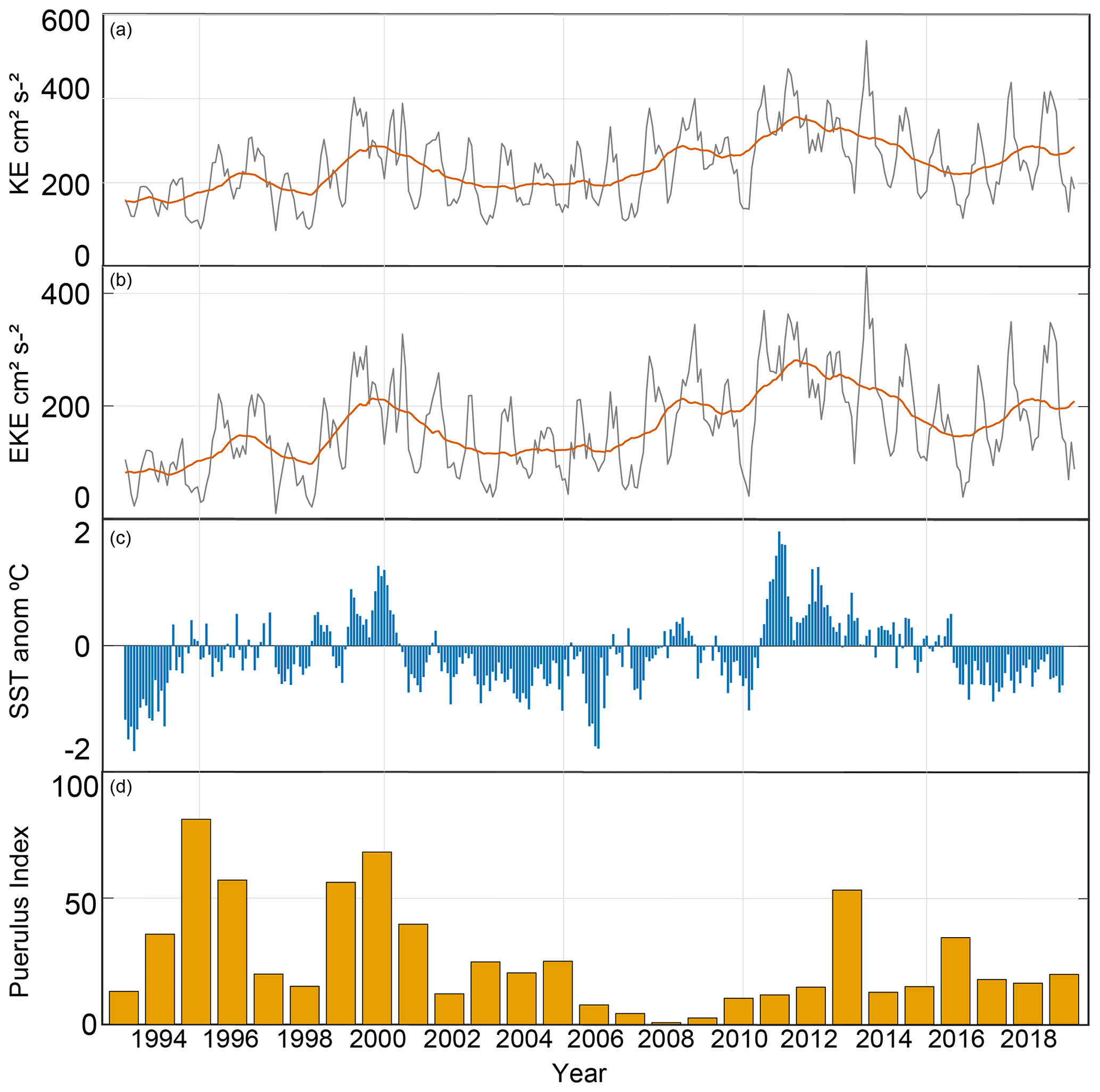
Figure 11 (a) Kinetic energy and (b) eddy kinetic energy (cm² s⁻²) from altimeter data, the (c) SST (^∘C) anomaly from SSTAARS, and (d) PI for the whole western rock lobster fishery.

Similarly, SST anomalies (Fig. 11) have periods of neutral conditions and below-average temperatures, respectively, from approximately 2000 to 2008 (Pattiaratchi and Hetzel, 2020). These extended low-activity conditions may have caused a shift in the conditions experienced by pelagic western rock lobster larvae. The patterns may be due to atmospheric and oceanic processes that imprint themselves upon the SST field. The ocean's thermal energy is transferred to the atmosphere via the sea surface, which the SST controls. Thus, SST on a spatial scale plays a crucial role in regulating climate and variability. The extended period of cooler SST anomalies may have contributed to the low 2008 and 2009 settlements. A decreasing PI over the start of the century was in line with these patterns. Then recovery followed the maxima experiences with the 2011/12 La Niña (Boening et al., 2012), which perhaps took the system some years to return to conditions as usual. Thus, it may not be a season-specific factor that caused the years of low settlement in the late 2000s. Instead, consecutive years of these hiatus conditions (Fig. 11) have driven a regime shift in the environment, impacting P. cygnus pelagic life stages (DeYoung et al., 2004).

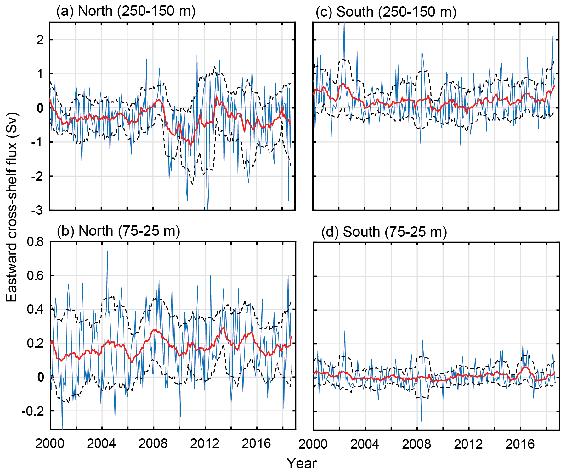
Figure 12 Cross-shelf transport (easterly) between 2000 and 2018 off the shelf. North and south divides are shown in Fig. 1a. North cross-shelf flux between (a) 250–150 m and (b) 75–25 m. South cross-shelf flux between (c) 250–150 m and (d) 75–25 m. The yearly moving mean (red) and the positive and negative moving standard deviations (dashed black) are included.

Despite cross-shelf transport being a forcing mechanism behind larval transport into the nearshore, a lack of statistical relationships was found through the multiple regression analysis. Given the hiatus conditions or shift after 2008 in the LC, one would expect some form of accompanying change in cross-shelf flux (Pattiaratchi and Hetzel, 2020). Over the 50 m contour, there are no noticeable inter-annual changes over the 18 years between the south and north boxes. In the south, there is minor variation in the standard deviation from the mean (Fig. 12, dashed lines); however, it is predominantly onshore transport on the shelf (50 m) and over the continental shelf (200 m). The cross-shelf transport in the north shows an apparent increase in variability over the continental shelf (Fig. 12, 200 m) after 2008, highlighting the increased movement in water over the northern part of the fishery (Fig. 12). This is also where the LC increases over the summer (Fig. 5b) and puerulus settlement shifts.

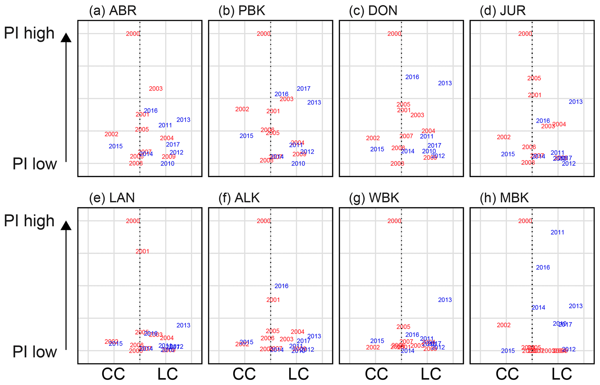
Figure 13 Relationship of the more dominant current during the early spring–early summer (September–November) to early PI at monitoring sites (a) Abrolhos, (b) Port Gregory, (c) Dongara, (d) Jurien Bay, (e) Lancelin, (f) Alkimos, (g) Warnbro, and (h) Cape Mentelle. The x axis is the difference between the LC and CC standardized, providing an indication of which is more prominent at the time. Red indicates the seasons before the recruitment failure, and blue indicates seasons after.

4.3.2 Seasonal: Capes Current and Leeuwin Current interactions during summer

Before 2008, conditions were reasonably neutral over the early settlement season, leading to high and low puerulus settlement potentially controlled by oceanographic and biological factors (Fig. 13). Since 2009, the LC has dominated (blue years skewed to the right, Fig. 13), possibly causing average to low puerulus conditions across all sites, except for Cape Mentelle, the southernmost site and potentially most isolated from the LC (Fig. 14h). Comparatively, over the late period of settlement (Fig. 14), the CC dominates the system, with higher settlement occurring later in the summer. Thus, the years of recruitment failure have neutral conditions where neither the CC nor LC is particularly dominant over the latter portion of the season. The same exists for 2007 and 2008 during the early portion of the season. Interestingly, during these recruitment failure years, the spatial extent of the LC during spring months was more considerable or on par with the 6 months prior, when newly hatched phyllosoma transport across the shelf into the open ocean may have also been impacted (Huang and Feng, 2015).

These patterns suggest that perhaps a timing mismatch is in play, suggested previously by de Lestang et al. (2015). While puerulus are crossing the shelf, an increase in LC strength may transport them past Cape Mentelle, away from suitable habitats. In contrast, a strong CC is likely to assist transport northward along the shelf, increasing settlement over the later season. Interaction between these two critical currents over the shelf influences the movement of puerulus onshore and needs to be investigated in greater detail. Particle tracking modelling over these months would be a possible way to investigate these interactions; however, this is beyond the scope of the present study.

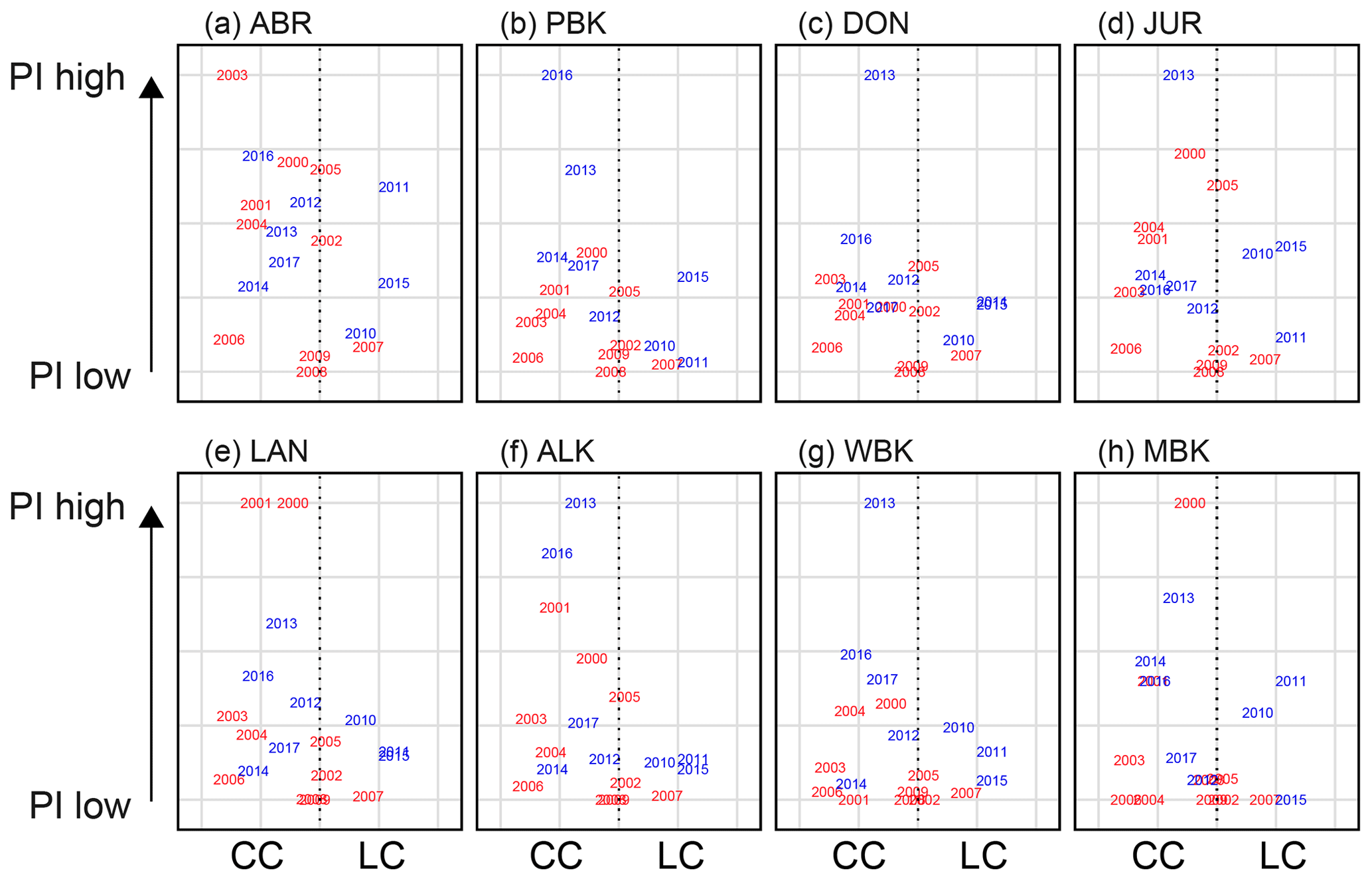
Figure 14 Relationship of the more dominant current during the late summer–early autumn (December–March) to late PI at monitoring sites (a) Abrolhos, (b) Port Gregory, (c) Dongara, (d) Jurien Bay, (e) Lancelin, (f) Alkimos, (g) Warnbro, and (h) Cape Mentelle. The x axis is the difference between the LC and CC standardized, indicating which is more prominent at the time. Red indicates the seasons before the recruitment failure; blue indicates seasons after.

5 Conclusions and implications

The objective of the current study was to determine oceanographic and biological factors that may explain the previously unexplained failure of puerulus settlement (2008–2009) and subsequent change in the proportions of puerulus settling in early vs. late parts of the season (Kolbusz et al., 2021). The study was completed through an exploratory multiple regression analysis encompassing direct oceanographic and biological factors likely to influence the pelagic early life cycle of P. cygnus. The main conclusions were as follows.

• Local oceanographic and biological conditions greatly influence P. cygnus, as settlement of puerulus at adjacent sites along the coast tend to be influenced by similar oceanographic and biological variables. Offshore, the Abrolhos Islands had a unique yet consistent pattern of settlement that correlated with particular oceanographic and biological factors.

• On a fishery-wide scale, the period of recruitment failure (2008 and 2009) and the associated low settlement period (2004–2010) coincided with a hiatus period in the Leeuwin Current system. This was associated with mainly neutral ENSO conditions and slightly cooler SST anomalies.

• Increased KE in the northern region of the fishery was negatively correlated to puerulus settlement in the early period of the season, whilst the KE (and EKE) in the southern region was positively correlated at selected sites. This suggests different driving mechanisms over the whole range of latitudes that encompass the fishery for settlement early and later in the season.

• Seasonal variation in the LC system likely controls the conditions that favour increased puerulus settlement. During the summer months of hatching, a strong LC negatively affects puerulus settlement at central sites after their pelagic phase. During the subsequent winter, the system is dominated by a strong southward LC and its associated eddies, which then assists onshore phyllosoma transport. Then, whilst the newly metamorphosed puerulus are moving onshore across the LC, should it be too strong, the current can negatively impact settlement at the northern sites but positively impact the southern sites.

• An increase in the strength of the LC in the summer months since 2006, combined with a decrease in the strength of the CC over the early summer months, may have caused a timing mismatch for puerulus settling on nearshore reefs. If the LC were stronger in summer, a strong CC would be needed to counteract the southward flow to get the puerulus transported northward, which has occurred in recent years. However, the CC in the latter half of the summer has been less variable and has not declined to the same extent, potentially explaining the trend of better settlement later in the season.

• Between 2008 and 2011, the cross-shelf transport in the northern half of the fishery across the continental shelf became more variable whilst being consistently offshore. This overlap with the period of recruitment failure suggests that cross-shelf transport in an offshore direction could have reduced the transport and subsequent settlement of puerulus onshore.

These findings have implications for fishery management and their modelling of future stocks of catchable western rock lobsters. Environmental conditions are suspected of altering the puerulus settlement, which can be incorporated into planning and management. For example, reductions in the fishing effort can encourage an increase in larvae for the following season (de Lestang et al., 2015).

This study offers insight into factors potentially behind the recruitment failure that have not been addressed before. It also expands our current understanding of what oceanographic variables potentially influence puerulus settlement and how the variables themselves are intertwined in this complex system. With the available numerical modelled data, we can show that it is not solely the LC that is the dominating factor behind puerulus settlement variability but also the CC, cross-shelf flow, and system state as a whole.

Appendix A

Table A1 Oceanographic data sources and sites used to calculate the 40 predictor variables included in time series analysis. Unless stated, the timing is within the season of puerulus settlement. Spawning season indicates that the variable is from the year prior or within the spawning season as larvae hatch.

Appendix B

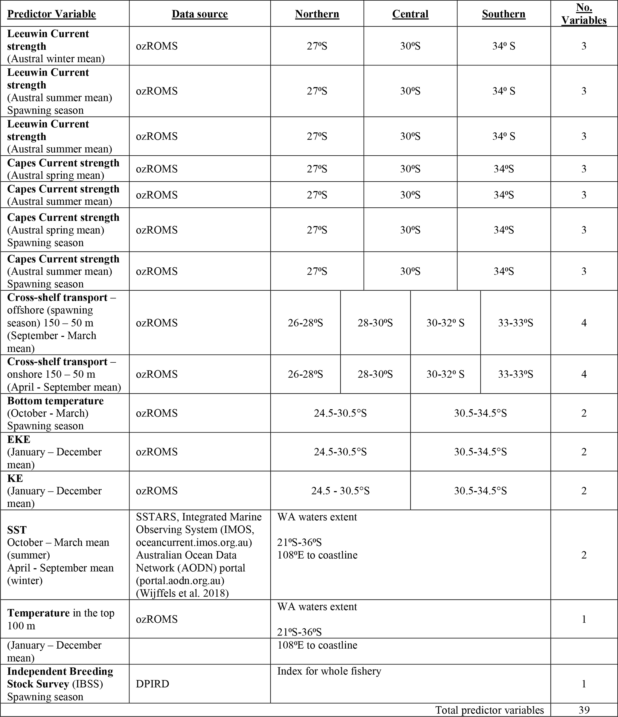
Table B1 Top generalized additive models (GAMs) for predicting the early puerulus settlement at the eight sites from full subset analyses. Differences between lowest reported corrected Akaike information criterion (ΔAICc), AICc weight (ωAICc), variance explained (R²), and effective degrees of freedom (EDF) are reported for model comparison. Model selection was based on the most parsimonious model (fewest variables) within two units of the lowest AICc, and models are ordered by parsimony.

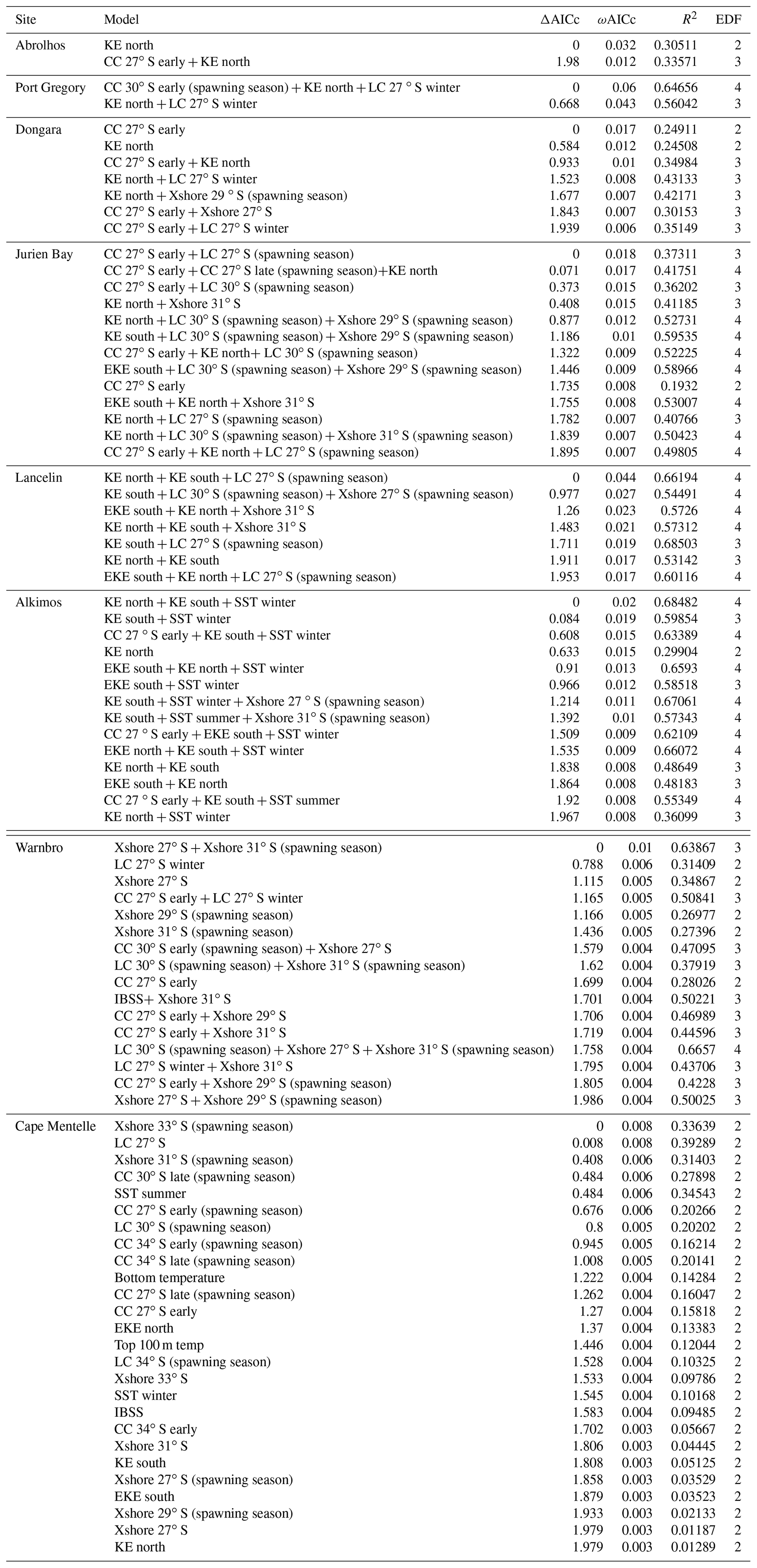
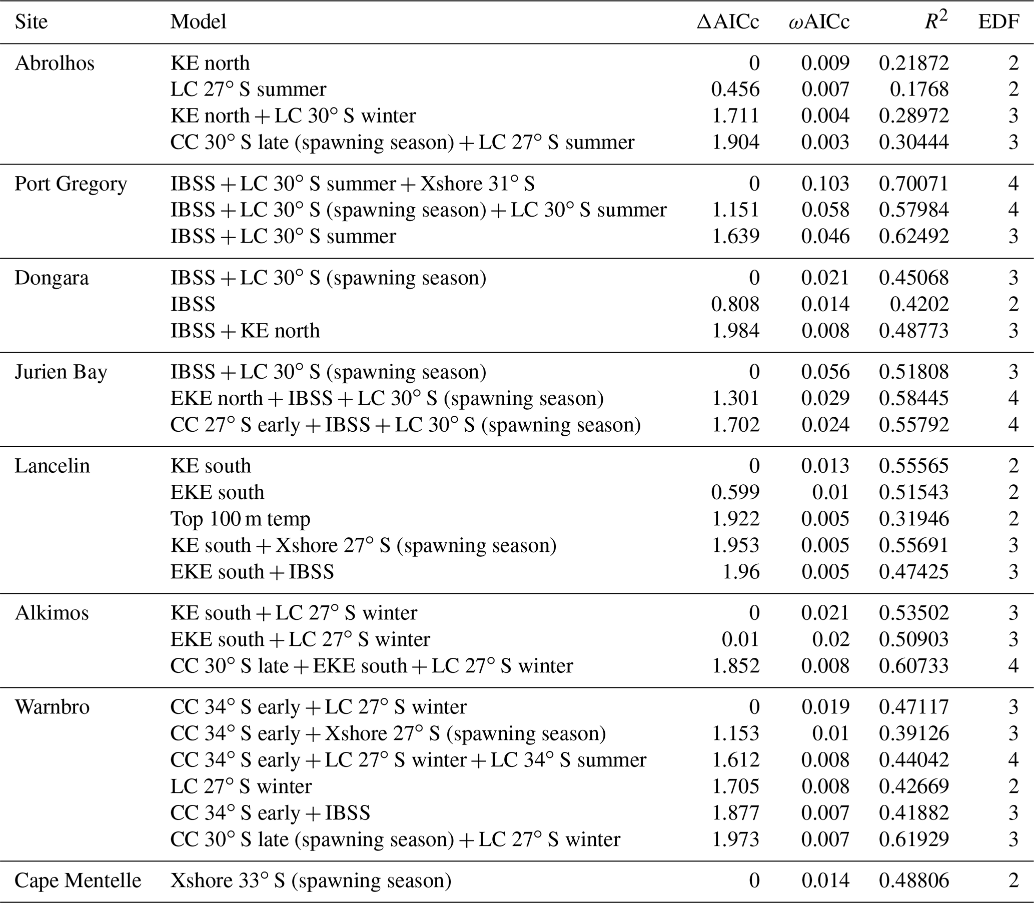
Table B2 Top generalized additive models (GAMs) for predicting the late puerulus settlement at the eight sites from full subset analyses. Differences between lowest reported corrected Akaike information criterion (ΔAICc), AICc weight (ωAICc), variance explained (R²), and effective degrees of freedom (EDF) are reported for model comparison. Model selection was based on the most parsimonious model (fewest variables) within two units of the lowest AICc, and models are ordered by parsimony.